Tests of goodness of fit to multiple data sets

Abstract

We propose a new and rather stringent criterion for testing the goodness of fit between a theory and experiment. It is motivated by the paradox that the criterion on $\chi^{2}$ for testing a theory is much weaker than the criterion for finding the best fit value of a parameter in the theory. We present a method by which the stronger parameter-fitting criterion can be applied to subsets of data in a global fit.

1 Introduction

Global fits of theory to large amounts of experimental data are rather important to current elementary particle phenomenology [1, 2, 3]. A substantial amount of work has been done to estimate the errors on these fits [4, 5, 6, 7], and it is now of obvious importance to test whether the fits obtained are actually good. Is the theory correct? Or is an extension to the standard model needed? Are the experiments correct?

The simplest requirement for a good fit is that the overall $\chi^{2}$ indicates a good fit according to the hypothesis-testing criterion, which allows a range $\sim\!\sqrt{2N}$ in the value of $\chi^{2}$ (where $N$ is the number of degrees of freedom). In fact, as we will show, this criterion is far from optimal. For example, a small subset of the data may be quite badly fit, but the contribution of that subset to the overall $\chi^{2}$ may nevertheless be too small for it to show up significantly.

In this paper we propose a new criterion for goodness of fit. Not only should the overall $\chi^{2}$ be good, but the fits to individual experiments in the data set or to subsets of the data should also be good in a particular and quite stringent manner. This leads to a “parameter-fitting” criterion that goes beyond the traditional “hypothesis-testing” criterion.

Figure 1: Hypothetical plot of $\chi^{2}$ vs. parameter $p$ in fitting of theory to data with $N=100$ points.

Our criterion is motivated by the following paradox [8], the “paradox of parameter determination and hypothesis testing” which is illustrated in Fig. 1. If one has a theoretical prediction for an experiment with $N$ data points, then a good fit should have $\chi^{2}$ approximately in the range $N\pm\sqrt{2N}$, which is the one-standard-deviation range for $\chi^{2}$ when the experiment is repeated many times. Let us call this the hypothesis-testing criterion. On the other hand, if the theory has a parameter $p$ that is fitted from the data, then the one-standard-deviation error on that parameter is given by a deviation of $\chi^{2}(p)$ by one unit from its minimum. Let us call this the parameter-fitting criterion. Now observe that if $p$ is varied so as to give a deviation of $\sqrt{2N}$ of $\chi^{2}(p)$ from its minimum, it produces a large deviation of $(2N)^{1/4}$ standard deviations from the best fit. The paradox is that a particular value of $p$, such as $p_{2}$, can thus simultaneously provide a good fit according to the hypothesis-testing criterion and a bad fit according to the parameter-fitting criterion.

The paradox is resolved by examining what happens if the experiment is repeated—see Fig. 2. The curves for $\chi^{2}(p)$ fluctuate vertically by a typical amount $\sqrt{2N}$, but horizontally only by a typical amount corresponding to a one-standard-deviation variation in the parameter. If one only knows the predictions of the theory for one particular value of $p$, then only the weaker hypothesis-testing criterion ($\chi^{2}$ in the range $N\pm\sqrt{2N}$) can be used. But if more information is available, namely the predictions of the theory for any value of $p$, then the shape of the $\chi^{2}(p)$ curve can be used, and hence a more stringent criterion for goodness of fit is available.

Figure 2: Typical plots of $\chi^{2}(p)$ when the experiment of Fig. 1 is repeated.

In order to test the goodness of fit to a set of experimental data, one should obviously examine not only the overall total $\chi^{2}$, but also the $\chi^{2}$ for suitable subsets of data. Our aim in this paper is to find the most stringent criterion for doing this. First, we will introduce the key idea by means of a simple example, and we will show that the appropriate criterion is a version of the parameter-fitting criterion rather than the weaker hypothesis-testing criterion. Then we will generalize the resulting criterion to a full multi-parameter and multi-experiment situation. Finally we will present a convenient method for showing the results in one-dimensional plots when there are many theoretical parameters, and examine those plots for a typical application that is of current interest.

In addition to the standard concepts of statistical and systematic errors, we find it useful to introduce the concept of a bug: an unforeseen error that is not taken into account in the determination of the systematic errors, and for which the probability distribution is highly non-Gaussian. A bug in a computer program used in the experiment or in the theory calculation is a canonical example. But we also find it useful to consider an error in the theory itself as a bug: an error in the Lagrangian instead of in hardware or software. An error in the theory is otherwise known as new physics. An actually incorrect experiment is also an example of a bug.

The reason for explicitly introducing the concept of a bug is to suitably describe what happens when there is an extremely bad fit between theory and experiment. In this situation, our usual experience is not that an extremely improbable fluctuation has occurred in the normal statistical and systematic effects, but that something has happened that wasn’t allowed for in the estimation of the errors, i.e., a bug has occurred.

The observed distribution of errors found in a study of actual experiments in particle physics does not in fact follow a Gaussian form [9]. Although the peak of the distribution is that of the expected Gaussian—showing that experimentalists typically estimated their one-standard-deviation errors correctly—there is a substantial non-Gaussian tail that one could associate, at least in part, with the bugs mentioned above.

We see at least two ways to formulate these ideas in terms of a statistical analysis. The first is simply to formulate an appropriate criterion for recognizing when a fit is bad. That is the primary issue addressed in this paper. A second approach, discussed in a separate paper[10], is to modify the normal formula for $\chi^{2}$ to take into account the non-Gaussian tails of error distributions. This improves the estimation of parameter values by allowing the fitting procedure to effectively disregard data points that are badly fit by the combination of theory and the other experiments. Such an analysis can also be used in a suitably Bayesian sense to deduce the probability of a bug, if the non-Gaussian tails are identified with the effects of bugs.

2 Two experiments; one parameter fit

We will explain our ideas in their simplest context, by presenting a hypothetical situation involving the comparison of a theory to two experiments.

Scenario

Consider two experiments, which we will call the TEV experiment and the HERA experiment. Let the relevant theory be given by standard perturbative QCD calculations with particular sets of parton densities, CTEQ and MRST, which have been fit to other data. Although the numbers we give are completely hypothetical, we use names representing actual experiments and actual parton densities in order to show vividly that we intend our ideas on statistical methods to be applied to important practical cases.

	TEV	HERA	Total
PDF	(100 points)	(100 points)	(200 points)
CTEQ	85	115	200
MRST	115	85	200

Table 1: Hypothetical values of $\chi^{2}$ for comparison between theory, using two different sets of parton distribution functions (PDF), and two sets of experimental data.

Suppose each data set consists of 100 points, and that the values of $\chi^{2}$ are as shown in Table 1. Clearly, each set of parton densities is a good fit to both experiments according to the obvious criterion, that for hypothesis testing.

But in fact, as we will now show, both sets of parton densities are actually bad fits to the data. We will show this by converting the problem to one of parameter fitting. Given the pair of parton density sets, any linear combination of them

$$f_{p}=pf^{\rm CTEQ}+(1-p)f^{\rm MRST}$$ (1)

is also a valid parton density set. Since the original CTEQ and MRST sets give good fits to previous data, we should expect that the new parton densities also give good fits to previous data, if $p$ is in a reasonable range, say $-1$ to 2.

We now ask for the results of a fit for $p$. Let us hypothesize that the $\chi^{2}$ functions for the two experiments are quadratic functions of $p$, and that they have the following forms, which reproduce the values in Table 1:

$$\chi_{\rm TEV}^{2} = 85+30(1-p)^{2}$$

$$\chi_{\rm HERA}^{2} = 85+30p^{2}\;.$$ (2)

The total chi squared is

$$\chi_{\rm tot}^{2}=\chi_{\rm TEV}^{2}+\chi_{\rm HERA}^{2}=185+60(p-0.5)^{2}\;.$$ (3)

The best fit has $p=0.5\pm 0.13$, and the corresponding best parton density set is $f^{\rm best}\equiv f_{0.5}\,$.

Global fit in the scenario is not correct

We now see that the hypothetical CTEQ and MRST parton densities are both about 4 standard deviations from the best fit, and are therefore both strongly disfavored, as claimed above. We can obtain the same result by considering the fits to $p$ that would be performed by the individual experiments. TEV says that $p=1.00\pm 0.18$, while HERA says that $p=0.00\pm 0.18$. These results are inconsistent at the $3.9\,\sigma$ level.

We have moved a long way from the situation apparently given by the numbers shown in the last column of Table 1, where the hypothesis-testing criterion says that both the CTEQ and MRST parton densities give good fits to the data. By using the extra information that there is a parameter that can be fitted, we have invoked the much more powerful parameter-fitting criterion for goodness of fit, and have correctly concluded that there is an inconsistency. The real situation is probably that one (or both) experiments is wrong, or that the theoretical calculation for one (or both) experiments is wrong.

Since one of the experiments is wrong or has an incorrect theory calculation, the correct estimate of the value of the parameter is obtained from the fit to the other experiment. However, we do not know which experiment is the culprit. Thus the correct estimate of the fitted parameter is not the value $p=0.5\pm 0.13$ obtained from the global fit. Rather it is either $p=0\pm 0.18$ or $p=1\pm 0.18\,$. Our analysis cannot tell which of these two values is correct, because it does not tell us which data or which theoretical calculation should be discarded. To proceed in this case, we must investigate each experiment and its theory to discover what is wrong. In the meantime, we would have to make do with the range $p=0.50\pm 0.68$ that includes both experiments.

Even that extended range may not include the true situation, since an important possibility is that both experiments are incompatible with the theory, in which case the whole global fit to the TEV and HERA data is inapplicable. This situation could arise, for example, if there is some new physics that is important for both of the new experiments but which is not accessible to the earlier experiments on which the CTEQ and MRST parton densities were based.

The particular values of $p$ that are preferred depend on the precise form for the $\chi^{2}$ for each experiment, which was hypothesized in Eq. (2). However, the fact that the experiments are inconsistent and that they prefer significantly different values of $p$ depends only on the values of $\chi^{2}$ in Table 1. That is, we do not actually need to do the parameter fitting to see that there is a problem. It is enough to show that the $\chi^{2}$ for one experiment can be reduced by many units in going from one parton density set to another, while the total $\chi^{2}$ for all of the experiments increases by only a small amount. According to the parameter-fitting criterion, there are therefore two parton density sets, each of which is strongly preferred over the other, by different sets of data.

Consequences of inconsistency

After deducing that an experiment is inconsistent with a theory calculation, we must try to figure out what went wrong. There is the usual list of suspects, including:

• An error in the experiment (e.g., a bug in the data analysis software), or any other kind of error in the experiment (e.g., an experiment that is simply wrong due to an unforeseen background or a mis-measured target size, to recall actual instances).

• A technical error in the theoretical calculations (e.g., a bug in software, or a QCD calculation taken to insufficiently high order in perturbation theory).

• New physics (i.e., an error in the Lagrangian used as a basis for the theory calculations).

As suggested before, we will label all of these as bugs, which are defined as infrequently occurring errors that were not allowed for when the systematic errors for the experiment and theory were estimated.

The kind of error that we call a bug can produce large effects on the cross section or on the theory calculation, so the distribution of effects due to bugs, considered over many experiments, is strongly non-Gaussian. Thus the estimate of probabilities from the quadratic approximation to $\chi^{2}$ is badly wrong for them. Since there is a single large source of error in such cases, we cannot appeal to the Central Limit Theorem to expect a Gaussian distribution.

Our analysis of $\chi^{2}$ for the experiments as a function of the parameter $p$ cannot tell us where the bug is. It merely tells us when it is likely that there is one. Given our previous experience with science, we know that the probability of a bug is non-negligible. Indeed, if we identify bugs with the non-Gaussian component of the distribution of experimental errors, then Bukhvostov’s results [9] imply that the probability of bugs in a certain class of high-energy physics experiments is about 15%! Not all of these bugs are readily identifiable. The identifiable bugs are those in the strongly non-Gaussian tail of the error-distribution. For example, Bukhvostov observes that 65 data points out of 933 have a deviation greater than $3\,\sigma$. That corresponds to about $7\%$ of the data, whereas a Gaussian distribution would predict only $0.3\%$.

Given a particular scenario, we have deduced that is likely (in an appropriately Bayesian sense) that there is a bug. Hence it is a correct scientific decision to investigate the experiments and the theory to locate the bugs. The issue for us now is how to quantify this decision more generally.

3 General case

In the previous section, we were able to diagnose that certain parton densities gave a bad fit to data because of the existence of two different sets of parton densities. Now we must ask how CTEQ could find the problem without MRST’s assistance (or vice versa). One method is to pick a significant parameter and to examine the dependence of $\chi^{2}$ on that parameter for particular experiments. An example of this for the MRST parton densities is given by Fig. 21 in Ref. [2], where $\chi^{2}$ for different experiments is plotted against $\alpha_{s}(M_{Z}^{2})$. In the scenario of the previous section, the comparison of two sets of parton densities also focused our attention on a different particular parameter.

But in a typical global fit, there are many parameters. So the issue we now address is how to automatically find the optimal combinations of parameters for detecting a bad fit.

We therefore consider a general situation in which we have many data points and experiments, and many parameters in the theory. We will choose ahead of time to divide the data into subsets. These subsets could be individual experiments, or data points obtained using similar experimental techniques, or data that rely on a specific aspect of theory. An example would be jet data from a particular experiment, possibly divided into regions of low, medium and high transverse energy. The idea is to choose subsets of data that are likely to be simultaneously affected by a typical bug. Let there be $g$ subsets (or groups) of data. The total $\chi^{2}$, which is a function of the theory parameters ${\bf p}$, is the sum of the $\chi^{2}$ for the individual subsets:

$$\chi_{\rm tot}^{2}({\bf p})=\sum_{i=1}^{g}\chi_{i}^{2}({\bf p})\;.$$ (4)

If necessary, the formula for $\chi^{2}$ may be fudged to take into account badly estimated correlated systematic errors, as is common practice in global fits for parton densities [6].

We want to ask whether the fit is improbable at some level, $c\%$. We might choose $c\%=5\%$ or even $c\%=10\%$ as the level below which further investigation is warranted. Our proposal is as follows:

1. Apply normal methods to find the best fit, with ${\bf p}={\bf p}_{\rm best}$ defined by the minimum of $\chi_{\rm tot}^{2}({\bf p})$.

2. If $\chi_{\rm tot}^{2}({\bf p}_{\rm best})$ is too high according to the hypothesis-testing criterion, with $P<c\%$, then we have a bad fit.

3. Similarly if for one or more of the individual experiments, $\chi_{i}^{2}({\bf p}_{\rm best})$ is too high according to the hypothesis-testing criterion, then again we have a bad fit. (In the case that only one experiment is a bad fit, the border line to declare a bad fit is more stringent than for the overall fit: The probability would have to satisfy $P<c\%/g$ to be considered a bad fit, because the bad fit could have occurred in any of $g$ places.)

4. Now let us define the region of an overall good fit as the region where $\chi_{\rm tot}^{2}({\bf p})-\chi_{\rm tot}^{2}({\bf p}_{\rm best})$ is less than about $\sqrt{2N}$, where $N$ is the total number of data points. It is not necessary to be too precise about this region. It only forms a basis for further exploration of goodness or badness of fit. One does not want to investigate values of the parameters that are much outside this region, because they then give an unambiguously bad fit. In addition, one can exclude parameter values that are known on other grounds to be physically wrong or implausible.

5. Find the minimum of each $\chi_{i}^{2}({\bf p})$, for the subsets of data, when the parameters range over the region just defined. (This is easily done by using the method of Lagrange multipliers.) Let the resulting minimum values be $\chi_{i,{\rm min}}^{2}$.

6. Now compute the difference between the $\chi_{i}^{2}$ at the best global fit and the minimum that was just calculated, i.e., $\chi_{i}^{2}({\bf p}_{\rm best})-\chi_{i,{\rm min}}^{2}\,$. If one or more of these is above a threshold for a bad fit, in the sense of parameter fitting, then the fit is bad.

Steps 5 and 6 are the novel parts of our proposal. A possible variation on these steps, based on mapping the variation of $\chi_{i}^{2}$ with $\chi_{\rm tot}^{2}$, is described in Sec. 5 and Appendix A. Whenever it is determined in one of these ways that a fit is bad, then further investigation is called for to attempt to discover the reason. Several caveats are in order:

• If a particular subset contains very few points and there are many parameters, it may be possible to get a $\chi_{i}^{2}$ much less than the number of points simply because there are many parameters. Typically, however, any particular subset of data determines only a few parameters; perhaps only one. We do not address here how to determine the relevant number of parameters or to determine what effect that has on our criterion.

• A literal use of our criterion requires that the error estimates be valid. In particular the correct correlated systematic errors must be used. However, it is common that properly correlated systematic errors are not available for experiments, and in that case some appropriate allowance must be made.

4 Presentation of results in one-dimensional graphs

The exploration of the parameter space in many dimensions is difficult to visualize. One way to study it is to select a particularly significant parameter and plot the $\chi_{i}^{2}$ for each experiment as a function of that parameter, while the other parameters are continuously adjusted to optimize the fit. Examples of such plots are to be found in Refs. [2, 6].

However, this procedure is really only useful when one has identified a particularly significant direction in parameter space. So we now propose a more general way to plot the results. In fact, we propose two ways to make the plot, because it is unclear to us at this stage which form will be more useful.

4.1 Plot of $\chi_{i}^{2}$ against $\chi_{\rm tot}^{2}$

In the first method, for each value of $\chi_{\rm tot}^{2}$ we plot the minimum of $\chi_{i}^{2}({\bf p})$ that is compatible with that value of $\chi_{\rm tot}^{2}$. We thus obtain curves of the $\chi_{i}^{2}$ for each particular experiment against the total $\chi^{2}$. One can read off from the plots how well these experiments agree with the overall global fit.

Rough sketches of hypothetical examples of such plots are shown in Fig. 3. Curve A corresponds to an experiment that agrees with the global fit and strongly determines all of the parameters. Curves B and C correspond to experiments that agree with the global fit, but that do not determine all the parameters. Finally, curve D corresponds to an experiment that is in disagreement with the global fit. (Of course, this analysis cannot determine whether it is experiment D, one of the other experiments, or the theory that is in error.) The criterion that an experiment disagrees with the global fit is that its $\chi^{2}$ decreases by more than the amount allowed by the parameter-fitting criterion.

These curves are straightforward to compute by the Lagrange multiplier method (cf. [6]). One minimizes

$$f_{\lambda}({\bf p})\,=\,(\lambda-1)\,\chi_{i}^{2}({\bf p})\,+\,\chi_{\rm tot}^{2}({\bf p})$$ (5)

for various values of the parameter $\lambda$. Then for each value of $\lambda$, the corresponding values of $\chi_{i}^{2}$ and $\chi_{\rm tot}^{2}$ give one point on the graph. Performing the minimization of (5) gives a parametric representation of the curve of minimum $\chi_{i}^{2}$ against $\chi_{\rm tot}^{2}$.

\psfrag{chi2i}{$\chi_{i}^{2}$}\psfrag{chi2min}{$\chi_{\rm min}^{2}$}\psfrag{chi2total}{$\chi_{\rm tot}^{2}$}\psfrag{A}{A}\psfrag{B}{B}\psfrag{C}{C}\psfrag{D}{D}\includegraphics[scale={0.7}]{eps/chi2-chi2-v3.eps}

Figure 3: Possible results of plotting $\chi_{i}^{2}$ for subsets of data as a function of $\chi_{\rm tot}^{2}$.

Curves such as those in Fig. 3 would be generated using $\lambda>1$ in (5), so that experiment $i$ is weighted more heavily than in the Best Fit, and hence its $\chi_{i}^{2}$ is reduced relative to its value at the global minimum. Meanwhile, it is also useful to minimize $f_{\lambda}({\bf p})$ using $\lambda$ in the range $0<\lambda<1$, since that reveals how the fit to all the other experiments (as measured by $\chi_{\rm tot}^{2}-\chi_{i}^{2}$) can be improved when the fit to experiment $i$ is allowed to get worse (as measured by an increase in $\chi_{i}^{2}$). This region can be included in graphs like those illustrated in Fig. 3, where it adds an additional branch to each curve, beginning at $\chi_{\rm min}^{2}$; but we defer it instead until Sec. 4.2.

General expectation: monotonic decrease is normal

As we will now explain, a curve like B is unlikely. In that curve, the $\chi_{i}^{2}$ for the experiment decreases slightly and then increases again as $\chi_{\rm tot}^{2}$ increases. The most common situation is probably curve C, where the $\chi_{i}^{2}$ for the experiment decreases slightly with the global $\chi_{\rm tot}^{2}$; and never rises again, at least not in the relevant range of $\chi_{\rm tot}^{2}$.

The reason for this is that one experiment normally only determines a fraction of the parameters in a global fit. For example, a neutrino DIS experiment with a limited range in $Q^{2}$ tells us a lot about the flavor-separated quark and antiquark densities, but says relatively little about the gluon density and the value of $\alpha_{s}$. On the other hand, a jet production experiment at a hadron collider constrains the gluon density and $\alpha_{s}$, but does little to discriminate the flavors of quarks and antiquarks.

If we choose a value of $\chi_{\rm tot}^{2}$ that is just a small amount above the minimum, then only a limited range of parameters is allowed. As we increase the chosen value of $\chi_{\rm tot}^{2}$, the range for the parameters increases. This implies, for example, that the parameters for the quark densities can be adjusted to give a better fit to the neutrino experiment. At the same time, the large value of $\chi_{\rm tot}^{2}$ is maintained by having a poor form for the gluon density. Since the bad gluon density gives hardly any contribution to the $\chi_{i}^{2}$ for the neutrino experiment, the $\chi_{i}^{2}$ for the neutrino experiment will decrease as $\chi_{\rm tot}^{2}$ increases.

This situation is general, since it is normal that individual experiments and subsets of data strongly determine only a subset of parameters. Thus the curves in Fig. 3 will commonly fall monotonically with $\chi_{\rm tot}^{2}$, as in curves C and D. A rising curve like A or B will only occur for a subset of data that significantly constrains all of the parameters. At the boundary where $\chi_{\rm tot}^{2}$ approaches its minimum value, the curves always become vertical, since the derivative of $\chi_{\rm tot}^{2}$ with respect to any parameter must be zero at the minimum.

Note that a mildly varying curve like B or C is quite normal in a good fit. It indicates that the experiment or subset of data in question is compatible with the global fit but that it does not determine all the parameters. The subset of data might nevertheless be the most significant in determining some subset of the parameters.

4.2 Plot of $\chi_{i}^{2}$ against $\chi_{{\rm not\,}i}^{2}$

A second method to visualize the character of the global fit is to plot the minimum of $\chi_{i}^{2}$ not against the total $\chi^{2}$, but against the $\chi^{2}$ for the remaining data, i.e. against

$$\chi_{{\rm not\,}i}^{2}\equiv\chi_{\rm tot}^{2}-\chi_{i}^{2}=\sum_{j\neq i}\chi_{j}^{2}\;.$$ (6)

This has the advantage of relating two independent contributions to the total $\chi^{2}$, and gives the plot some simple but interesting mathematical properties in a neighborhood of the overall best fit.

This curve can be extracted from the same Lagrange multiplier results that were used in the previous method, since the quantity (5) that was minimized there can be written as

$$f_{\lambda}({\bf p})=\lambda\chi_{i}^{2}({\bf p})+\chi_{{\rm not\,}i}^{2}({\bf p})\;.$$ (7)

Minimizing $f_{\lambda}$ with respect to the theory parameters ${\bf p}$ gives the minimum of $\chi_{i}^{2}$ for some value of $\chi_{{\rm not\,}i}^{2}({\bf p})$. Varying $\lambda$ allows one to plot the minimum $\chi^{2}$ for experiment $i$ against $\chi^{2}$ for the other experiments; i.e., the curve is again defined parametrically as a function of $\lambda$. A typical form to be expected for the plot is shown in Fig. 4.

Figure 4: Possible results of plotting the minimum of $\chi_{i}^{2}$ for a subset of the data as a function of $\chi^{2}$ for the remaining data. The diagonal dashed line at $-45^{\circ}$ is tangent to the curve at the point where $\chi_{\rm tot}^{2}$ has its minimum value.

Let ${\bf p}(\lambda)$ be the position of the minimum of the function (7). The requirement of a minimum implies that for all small variations of the parameters ${\bf p}$ about ${\bf p}(\lambda)$, the variations of the two components of $\chi^{2}$ satisfy

$$\lambda\,\delta\chi_{i}^{2}+\delta\chi_{{\rm not\,}i}^{2}=0\;,$$ (8)

and hence on the curve being plotted

$$\frac{d\chi_{i}^{2}}{d\chi_{{\rm not\,}i}^{2}}=-\frac{1}{\lambda}\;.$$ (9)

It follows that the curve always has the qualitative shape shown in Fig. 4. The best overall fit corresponds to the point $\lambda=1$, for which the quantity being minimized is just $\chi_{\rm tot}^{2}$. This point corresponds to the geometrical situation shown on the graph, where a $-45^{\circ}$ line is tangent to the curve relating the two $\chi^{2}$s, as indicated by the dashed line. The portion of the curve to the right of the best fit is generated by $\lambda>1$, and carries the same information as Fig. 3. The region to the left is generated by $0<\lambda<1$, where experiment $i$ is de-emphasized in the fit, so that the other experiments are fit better while experiment $i$ is fit worse.

Figure 4 expresses a situation that is essentially the same as in our original scenario of the TEV and HERA data in Sec. 2. The roles of the TEV and HERA experiments are played by experiment $i$ and all-the-other-experiments. Exactly the same criterion for consistency should be applied: We have an inconsistency if, at the best global fit, $\chi_{\rm tot}^{2}$ exceeds the sum of the absolute minima for the two subsets of data by more than a few units (the parameter-fitting tolerance), i.e., if

$${\rm min}(\chi_{\rm tot}^{2})-{\rm min}(\chi_{i}^{2})-{\rm min}(\chi_{{\rm not\,}i}^{2})>\mbox{parameter-fitting tolerance}.$$ (10)

Of course, the same plot should also be made with experiment $i$ replaced in turn by each of the other experiments.

5 Application: CTEQ5

As a first practical application of the ideas presented here, we have examined the CTEQ5 parton distribution analysis [1]. Fig. 5 shows a realization of the generic Fig. 3 for the 8 experimental data sets that contribute the lion’s share of data points ($1115$ out of $1295$) to that analysis. The data sets are numbered in Fig. 3 in the order of decreasing consistency with the rest of the global analysis, as will be shown in Table 2. We subtract the best-fit values, and therefore plot

$$\Delta\chi_{i}^{2}=\chi_{i}^{2}-\chi_{i}^{2}(0)$$ (11)

versus

$$\Delta\chi_{\rm tot}^{2}=\chi_{\rm tot}^{2}-\chi_{\rm tot}^{2}(0)\;,$$ (12)

where the argument $(0)$ denotes values at the minimum of $\chi_{\rm tot}^{2}$.

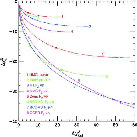
Figure 5: Variation of $\chi_{i}^{2}$ with $\chi_{\rm tot}^{2}$ for 8 of the data sets of the CTEQ5 parton density analysis. Dots mark the points found by $\lambda=5$ in Eq. (5).

Fig. 5 shows that for several of the data sets, $\chi_{i}^{2}$ can decrease by many units within the range of parameters for which $\chi_{\rm tot}^{2}$ increases by $\sqrt{2N}\simeq 50$. We conclude that the combined CTEQ5 data set is therefore not internally consistent according to the parameter-fitting criterion—even if we make a substantial allowance for the neglect of correlations among the errors used to define $\chi_{i}^{2}$. (It is also necessary to make an estimate of the expected decrease in $\chi_{i}^{2}$ given the total number of parameters and the degree to which they are determined by the experiment in question. But we do not do this here.)

Fig. 6 similarly shows a realization of the generic Fig. 4 for the same 8 data sets. The inconsistency between theory and these data sets according to Steps 5 and 6 of our parameter-fitting criterion is again apparent.

Figure 6: Variation of $\chi_{i}^{2}$ with $\chi_{{\rm not\,}i}^{2}$ for 8 data subsets of the CTEQ5 parton density analysis. Dots mark the points found by $\lambda=5$ for $\Delta\chi_{i}^{2}<0$, and $\lambda=0.2$ for $\Delta\chi_{i}^{2}>0\,$.

The curves in Figs. 5 and 6 were obtained by minimizing $f_{\lambda}({\bf p})$ of (5) with respect to the 16 free parameters ${\bf p}$ of the CTEQ5 fit, using approximately 18 values of the Lagrange multiplier parameter $\lambda$ for each data set $i$. As an aid to plotting smooth curves, these results were fitted to a simple two-parameter model that is described in Appendix A. That model was found to provide a good description of the variations of $\chi_{i}^{2}$ with $\chi_{{\rm not\,}i}^{2}$, while serving to smooth over small variations and numerical effects that are unimportant for our purposes.

The model of Appendix A also provides a direct measure of the internal consistency of the data sets. Specifically, its parameter $S$ measures the number of standard deviations by which the value of an effective parameter $q$, as measured by data set $i$, differs from its value as measured by the combination of all the other data sets. (Parameter $q$ represents the combination of fit parameters that data set $i$ is most sensitive to, in conflict with the other data sets. It is therefore a different—and generally nonlinear—function of the actual fit parameters for each data set.)

The fitted values of parameter $S$ are listed in Table 2. We see that many of these data sets are distinctly inconsistent with the rest of the data, since the parameter $S$ is considerably larger than $1.0\,$. Meanwhile, the parameter $\tan\phi$ is generally less than $1.0$, which indicates that each data set (with the exception of set $6$), is somewhat less effective in determining its parameter $q$ than is the remainder of the data sets put together.

The inconsistency of the data sets used for global fits to parton density has been known to practitioners for some time. It was quantified in [7] by a simple means of finding the decrease in $\chi_{{\rm not\,}i}^{2}$ that could be produced by removing data set $i$ from the fit. In our notation, that corresponds to the point $\lambda=0$, which provides the asymptote of minimum $\Delta\chi_{{\rm not\,}i}^{2}$ in Fig. 6.

Expt	$1$	$2$	$3$	$4$	$5$	$6$	$7$	$8$
$S$	$2.7$	$3.3$	$3.3$	$4.2$	$5.3$	$7.6$	$7.4$	$8.3$
$\tan\phi$	$0.56$	$0.54$	$0.99$	$0.86$	$0.71$	$1.14$	$0.65$	$0.39$

Table 2: Fits of Eqs. (17)–(18) for 8 of the experiments in the CTEQ5 analysis (numbered as in Figs. 5 and 6).

What to do about this situation—other than the long-term option of waiting for the discrepancies to be resolved by improvements in theory or experiment—remains an open question. In order to obtain provisional results in the interim, Ref. [7] advocated estimating the uncertainty of predictions based on the global fit as those contained in the region $\Delta\chi_{\rm tot}^{2}<T^{2}$, where $T\approx 10$ was chosen in order to assume a range of uncertainty for the predictions of the global fit that is somewhat broader than the variations of the experiments going into it, which are indicated in Table 2. Of course, any estimate of the uncertainties based on an inconsistent fit will necessarily be somewhat model-dependent.

There is reason to hope that at least one discrepancy will be resolved in the near future by new experimental data. That is between data sets $3$ and $5$, which correspond to data on $F_{2}$ from the two major HERA experiments H1 and ZEUS. These are similar physical measurements made by similar techniques, and yet we find that improving the fit to either of these two experiments (by emphasizing it in the fit with an appropriate Lagrange factor $\lambda$) makes the fit to the other experiment get worse. This suggests that the problem is an experimental error that may be resolved in the new data that is expected soon from these groups.

The largest values of the inconsistency parameter $S$ in Table 2 are produced by data sets $7$ and $8$, which are data from muon scattering on deuterium and neutrino scattering on a nuclear target. One may speculate that the problems are caused by inaccurate treatment of nuclear binding effects in these experiments, although the discrepancy associated with the $\mu d$ data is not much worse that associated with the $\mu p$ data measured by the same group.

One should be cautious in interpreting the value of $S$ as a definite number of standard deviations, since the interpretation derived in Appendix A assumes that only one effective parameter is determined by a particular experiment.

For the inconsistency to be a real effect, it should be confirmable in another global fit. That this is the case for the MRST fit can be seen in Fig. 21 of [2]. There $\chi^{2}$ is plotted as a function of $\alpha_{s}(M_{Z}^{2})$ for several experiments. The CCFR $F_{2}$ and the BCDMS $F_{2}^{\mu p}$ are clearly very inconsistent with the MRST fit, in agreement with our results. We also find a strong inconsistency with the BCDMS $F_{2}^{\mu d}$ data, but that data does not appear in the MRST plot.

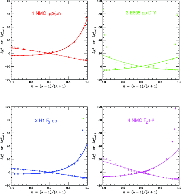
Figure 7: Variation of $\chi_{i}^{2}$ (solid curves) and $\chi_{{\rm not\,}i}^{2}$ for experiments 1–4.

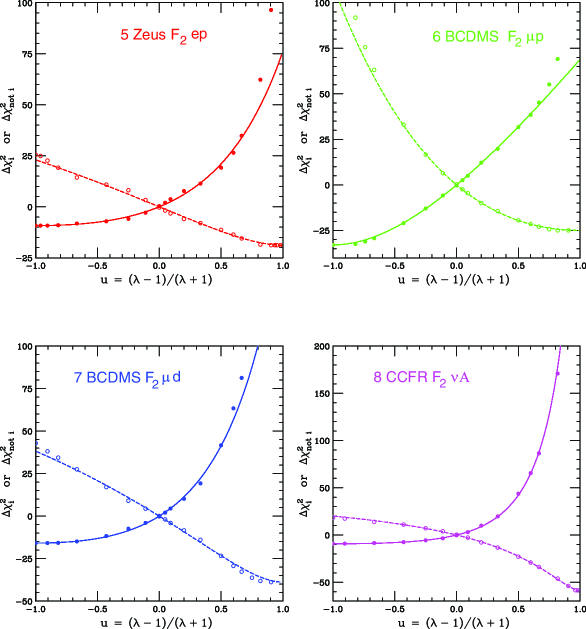
Figure 8: Variation of $\chi_{i}^{2}$ (solid curves) and $\chi_{{\rm not\,}i}^{2}$ for experiments 5–8.

6 A third kind of plot

The effective one-dimensional model of Appendix A suggests a new type of plot in which the various $\chi^{2}$ contributions are shown as a function of the Lagrange Multiplier parameter. In doing this, it is convenient to define $u=(\lambda-1)/(\lambda+1)$. This makes the function being minimized become $(1+u)\Delta_{1}+(1-u)\Delta_{2}$, which is more symmetric with respect to $\Delta_{1}=\chi_{i}^{2}$ and $\Delta_{2}=\chi_{{\rm not\,}i}^{2}$.

Results from the 8 experiments discussed previously are shown in Figs. 7 and 8. The fits using the one-dimensional (2 parameter) model are quite good, which lends confidence to the results from that model that are shown in Table 2.

This fitting can be thought of as finding the single parameter (a non-linear combination of the fit parameters) that each experiment is most sensitive to in disagreement with the other experiments.

7 Conclusions

A common problem with global fits is that if there is a bad fit to a particular experiment with few data points, its contribution to the total $\chi^{2}$ may be completely negligible according to the hypothesis-testing criterion. The bad fit to a few data points will not be noticeable in the goodness of fit as measured by the overall $\chi^{2}$. Our new criterion applies a parameter-fitting criterion to individual experiments, and hence can recognize when a bad fit to a single experiment is significant, even if that experiment has too few data points to make a big effect on the total $\chi^{2}$. A bad fit is detected if the experiment strongly determines any particular combination of parameters, and that determination is incompatible with the value determined by the other experiments.

In simple cases where there is only one parameter to measure, such as the mass of a particle, every one of a group of experiments can separately measure the parameter. Consistency between the experiments is just a matter of whether the measured values agree within errors. Of course, the new criterion proposed in this paper reproduces that result; but the extra complication it introduces is totally unnecessary for that situation.

The new criterion becomes important when there are many parameters to determine, but each experiment determines only a few combinations of them. Questions of consistency can then only be addressed after a global fit has been performed to determine all of the parameters. The more elaborate methods that we propose then become essential to optimally test consistency.

Our criterion can be expressed in an especially simple form whenever the dependence of the individual $\chi_{i}^{2}$ can be approximated by a quadratic function of the effective parameters, as is shown in Appendix A for a single effective parameter, and in Appendix B for an arbitrary number of parameters.

We have demonstrated how our criterion works when applied to an actual case of current interest, the global fit to determine parton densities.

Appendix A One-parameter quadratic model

In this appendix, we derive the relationship between $\chi_{i}^{2}$ and $\chi_{\rm tot}^{2}$ for the simple case that experiment $i$ determines just one combination of the fit parameters, and the dependence on that parameter can be approximated by a quadratic function in the region of $\chi_{\rm tot}^{2}$ that is of interest.

We will show that in this case, a well-defined shape is predicted for the graphs of $\chi_{i}^{2}$ vs. $\chi_{\rm tot}^{2}$, or $\chi_{i}^{2}$ vs. $\chi_{\rm tot}^{2}-\chi_{i}^{2}$. This shape is defined by two parameters; and the degree of consistency between experiment $i$ and the other experiments is given directly by one of those parameters. In Sec. 5, we found this shape to provide a good approximation for the study of fits of parton densities.

Since we are treating the case that experiment $i$ determines a single combination of parameters, we can define a transformation of the parameters, so that only a single parameter $p$ is relevant, and

$$\Delta\chi_{\rm tot}^{2} = \chi_{\rm tot}^{2}-\chi_{\rm tot}^{2}(0)\,=\,p^{2}$$ (13)

$$\Delta\chi_{i}^{2} = \chi_{i}^{2}-\chi_{i}^{2}(0)\,=\,(p^{2}-2pC)/D^{2}$$ (14)

where the argument $(0)$ denotes values at the minimum of $\chi_{\rm tot}^{2}$ as before. The method of transforming $\Delta\chi_{\rm tot}^{2}$ and $\Delta\chi_{i}^{2}$ to this form follows from the argument given in Appendix B. There should be an extra term in $\Delta\chi_{\rm tot}^{2}$ quadratic in the other parameters, but for our calculation this extra term is always set to its minimum value, and hence can be ignored. Solving for the dependence of $\chi_{i}^{2}$ on $\chi_{\rm tot}^{2}$ leads to

$$\Delta\chi_{i}^{2}=\frac{\Delta\chi_{\rm tot}^{2}}{D^{2}}-\frac{2C\sqrt{\Delta\chi_{\rm tot}^{2}}}{D^{2}}.$$ (15)

To interpret the two parameters $C$ and $D$ of this model, it is convenient to express them as

$$C = S/\!\tan\phi$$

$$D = 1/\!\sin\phi\;.$$ (16)

Rescaling the fit parameter by $q=p\,\sin\phi\,\cos\phi$ then leads to

$$\Delta\chi_{i}^{2} = \left(\frac{q}{\cos\phi}\,-\,S\cos\phi\right)^{2}\,-\,(S\cos\phi)^{2}$$ (17)

$$\Delta\chi_{{\rm not\,}i}^{2}=\Delta\chi_{\rm tot}^{2}-\Delta\chi_{i}^{2} = \left(\frac{q}{\sin\phi}\,+\,S\sin\phi\right)^{2}\,-\,(S\sin\phi)^{2}\;.$$ (18)

It is easy to read off from these formulae that experiment $i$ can be interpreted according to Gaussian statistics as a measurement of $q$ with result

$$q_{1}=S\cos^{2}\phi\,\pm\,\cos\phi\;,$$ (19)

while all of the other experiments combined give a result

$$q_{2}=-S\sin^{2}\phi\,\pm\,\sin\phi\;.$$ (20)

If we combine the errors in quadrature, these two results are seen to differ by

$$q_{1}-q_{2}=S\,\pm\,1\;.$$ (21)

Hence the two measurements differ by

$$S=\sqrt{\frac{C^{2}}{D^{2}-1}}$$ (22)

standard deviations. They are therefore consistent with each other if and only if $S\lesssim 1$, if a Gaussian distribution of errors is assumed. Meanwhile, the parameter $\tan\phi$ describes how effective experiment $i$ is at measuring the parameter $q$, compared to the combined effectiveness of the other experiments.

The relation between $\Delta\chi_{i}^{2}$ and $\Delta\chi_{{\rm not\,}i}^{2}$ in this model can be obtained explicitly by eliminating $q$ between Eqs. (17) and (18). The result is a parabolic curve which is seen in Figs. 5 and 6:

$$\Delta_{1}+\Delta_{2}\,=\,\left(\frac{\tan\phi\,\Delta_{2}\,-\,\cot\phi\,\Delta_{1}}{2\,S}\right)^{2}$$ (23)

where $\Delta_{1}\equiv\Delta\chi_{i}^{2}$ and $\Delta_{2}\equiv\Delta\chi_{{\rm not\,}i}^{2}$. This form holds in the region between the minimum of $\Delta\chi_{i}^{2}$ at $-(S\cos\phi)^{2}$ and the minimum of $\Delta\chi_{{\rm not\,}i}^{2}$ at $-(S\sin\phi)^{2}$. Outside that region, the curves do not exist.

In a more general example, with more parameters, but where each experiment only determines some of the parameters, the curves are no longer exactly of the form of Eq. (23). This can happen both because there are more parameters and because the quadratic approximation for the $\chi^{2}$ functions may break down, particularly far from the global minimum of $\chi_{\rm tot}^{2}$. This presumably accounts for the almost straight line behavior of the tails of some of the curves in Fig. 6.

Appendix B Quadratic approximation

It is instructive to assume that the various contributions $\chi_{i}^{2}$ which make up $\chi_{\rm tot}^{2}$ can be approximated by quadratic functions of the original fit parameters $\{x_{i}\}$ in the region of parameter space that is allowed by the hypothesis-testing criterion for $\chi_{\rm tot}^{2}$. This quadratic approximation has been found to be reasonably accurate in the case of parton density fitting [7]; and in any case it can provide a semi-quantitative guide to the kinds of behavior to be expected.

The first derivatives of $\chi_{\rm tot}^{2}$ vanish at its minimum, so in the quadratic approximation

$$\Delta\chi_{\rm tot}^{2}\,=\,\sum_{i,j}H_{ij}\,x_{i}\,x_{j}\;.$$ (24)

The real symmetric matrix $H$ has a complete orthonormal set of eigenvectors $V_{i}^{(k)}$:

$$\sum_{j}H_{ij}\,V_{j}^{(k)} = \epsilon_{k}\,V_{i}^{(k)}$$ (25)

$$\sum_{j}V_{j}^{(k)}\,V_{j}^{(\ell)} = \delta_{k\ell}\;.$$ (26)

Introducing new coordinates $\{y_{i}\}$ by

$$x_{i}\,=\,\sum_{k}y_{k}\,V_{i}^{(k)}/\sqrt{\epsilon_{k}}$$ (27)

leads to a simple diagonal expression:

$$\Delta\chi_{\rm tot}^{2}\,=\,\sum_{i}y_{i}^{2}\;.$$ (28)

The fit to a particular experiment, which we refer to here as experiment $1$, is measured by $\chi_{1}^{2}$. Since we assume that it is a quadratic function of $\{x_{i}\}$, it is also a quadratic function of $\{y_{i}\}$:

$$\Delta\chi_{1}^{2}\,=\,\sum_{i}A_{i}\,y_{i}\,+\,\sum_{i,j}B_{ij}\,y_{i}\,y_{j}\;.$$ (29)

Using arguments similar to the above, the real symmetric matrix $B$ has a complete set of orthonormal eigenvectors $W_{i}^{(k)}$:

$$\sum_{j}B_{ij}\,W_{j}^{(k)} = E_{k}\,W_{i}^{(k)}$$ (30)

$$\sum_{j}W_{j}^{(k)}\,W_{j}^{(\ell)} = \delta_{k\ell}\;.$$ (31)

Introducing new coordinates $\{p_{i}\}$, this time without a change in scale, by

$$y_{i}\,=\,\sum_{k}p_{k}\,W_{i}^{(k)}$$ (32)

creates a diagonal form for $\Delta\chi_{1}^{2}$ while preserving the very simple form for $\Delta\chi_{\rm tot}^{2}$:

$$\Delta\chi_{\rm tot}^{2}\, = \,\sum_{i}p_{i}^{2}$$ (33)

$$\Delta\chi_{1}^{2}\, = \,\sum_{i}(\widetilde{A}_{i}\,p_{i}\,+\,E_{i}\,p_{i}^{2})\;,$$ (34)

where $\widetilde{A}_{i}=\sum_{j}A_{j}W^{(i)}_{j}$. This result is identical to the form that was assumed in Appendix A, except that there is a sum of independent quadratic contributions in place of just a single one.

The relation between $\chi_{1}^{2}$ and $\chi_{\rm tot}^{2}$ under the quadratic assumption is easily found by choosing the parameters $\{p_{i}\}$ so as to minimize

$$f_{\omega}=\omega\,\Delta\chi_{1}^{2}\,+\,\Delta\chi_{\rm tot}^{2}\;.$$ (35)

The result is

$$p_{i}=\frac{-\omega{\widetilde{A}}_{i}}{2+2\omega E_{i}}\;.$$ (36)

Substituting (36) into (33)–(34) relates $\chi_{1}^{2}$ and $\chi_{\rm tot}^{2}$ parametrically via the Lagrange multiplier parameter $\omega=\lambda-1$.

References

- [1] H.L. Lai et al. [CTEQ Collaboration], Eur. Phys. J. C12, 375 (2000) [hep-ph/9903282].
- [2] A.D. Martin, R.G. Roberts, W.J. Stirling and R.S. Thorne, Eur. Phys. J. C4, 463 (1998) [hep-ph/9803445].
- [3] J. Erler and P. Langacker, “Electroweak Model and Constraints on New Physics” in: D.E. Groom et al., Eur. Phys. J. C15, 1 (2000).
- [4] W.T. Giele and S. Keller, Phys. Rev. D 58, 094023 (1998) [hep-ph/9803393].
- [5] J. Pumplin, D.R. Stump and W.-K. Tung, “Multivariate fitting and the error matrix in global analysis of data” [hep-ph/0008191].
- [6] D. Stump et al., “Uncertainties of predictions from parton distribution functions I: the Lagrange Multiplier method” [hep-ph/0101051].
- [7] J. Pumplin et al., “Uncertainties of predictions from parton distribution functions II: the Hessian method” [hep-ph/0101032].
- [8] L. Lyons, “Parameter Fitting And Hypothesis Testing And Detailed Examples Of Fitting Procedures,” OXFORD-NP-94/84.
- [9] A.P. Bukhvostov, “On the probability distribution of the experimental results” [hep-ph/9705387].
- [10] J. Pumplin, “Systematic errors, non-Gaussian statistics, and effective chi-squared”, manuscript in preparation.