Saturation at low $\mathbf{x}$

Abstract

This talk is an attempt to review all our knowledge on saturation at low $x$ both theoretical and experimental, to stimulate a search for saturation effects at THERA. The main goals of this presentation are

1.    To discuss an intuitive picture of the deep inelastic scattering that leads to the saturation of the parton densities;

2.    To show that the saturation hypothesis has solid theoretical proof;

3.    To report on the theoretical progress that has been made over the past two years in high parton density QCD, and on the property of the saturation phase that emerges from the theory that has been developed;

4.    To collect all that we know theoretically and experimentally about the saturation scale $Q_{s}(x)$ .

TAUP - 2681-2001

1 Introduction

At low values of $x$, QCD evolution, both DGLAP[1] and BFKL[2] , predict a striking increase of the parton densities which violate unitarity constraints [3]. Therefore, interactions between partons in the parton cascade, omitted in QCD evolution equations, should become essential to slow down the growth of the parton densities. We expect that these interactions will create an equilibrium -like system of partons with a definite value for the average transverse momentum, which we call a saturation scale ($Q_{s}(x)$). In other words, we expect a picture of a hadron as shown in Fig. 1[3, 4, 5, 6].

Figure 1: Picture of a hadron in the saturation region.

This talk is an attempt to review all our knowledge on saturation at low $x$ both theoretical and experimental, to stimulate a search for saturation effects at THERA. In spite of the fact that the high density QCD phase was only briefly discussed in the THERA Contribution to the TESLA TDR, everybody knows that if saturation effects are seen at THERA it will be the machine, while if not, it will remain one of many. The main goals of this presentation are

• To discuss an intuitive picture of the deep inelastic scattering that leads to the saturation of the parton densities;

• To show that the saturation hypothesis has solid theoretical proof;

• To report on the theoretical progress that has been made over the past two years in high parton density QCD, and on the property of the saturation phase that emerges from the theory that has been developed;

• To collect all that we know theoretically and experimentally about the saturation scale $Q_{s}(x)$.

Thera are two different ways to reach a high parton density phase: the first, is DIS at low $x$, the second is deep inelastic scattering on a nuclear target in which we have a rather large parton density from the beginning, due to a large number of nucleons in a nucleus. The best avenue to investigate the high density phase is to use both paths and to measure DIS on nuclei at low $x$. This is one of the THERA options and we will also discuss saturation phenomena for such a reaction.

2 Qualitative Picture of Interaction in DIS at low $\mathbf{x}$

2.1 Bjorken frame:

It is well known that deep inelastic scattering is most clearly visualized in a space-time picture in the Bjorken frame where the virtual photon has zero energy [7]. Therefore, in the Bjorken frame the electro-magnetic field is a standing wave with wavelength of the order of $1/q_{z}$ for a photon with four momentum $q_{\mu}=(0,q_{z},0,0,)$ (see Fig.  2). In this frame the fast hadron decays into a system of partons. Each parton has a longitudinal momentum $p_{i,z}=x_{i}P$, where $x_{i}$ is a fraction of the energy of incoming hadron carried by the parton, and a transverse momentum $p_{i,t}$. Due to the uncertainty principle each parton is localized in $\Delta z_{i}\approx 1/(x_{i}P)$ and, therefore, only partons with $x_{i}P\approx q_{z}$ can interact with the photon, since for all other partons the overlap integral is very small. In other words, the parton which interacts with the photon has $x_{i}\approx q_{z}/P$. Using the energy and momentum conservation for the parton - photon interaction one can easily obtain that $x_{i}P=q_{z}/2$ which gives $x_{i}=q_{z}/2P=q^{2}_{z}/2Pq_{z}=Q^{2}/2(P\cdot q)=Q^{2}/s=x_{Bj}$ at low $x$.

Figure 2: Parton cascade in the Bjorken frame.

The lifetime of the $i$-th parton is of the order of $\tau=\tau_{r.f.}\gamma=\frac{E_{i}}{p^{2}_{i,t}}=\frac{x_{i}P}{p^{2}_{i,t}}$ where the lifetime in the rest frame of the $i$-parton $\tau_{r.f.}=\frac{1}{p_{i,t}}$ and $\gamma=\frac{E_{i}}{p_{i,t}}$. The parton that interacts with the photon lives for a short time $\approx 1/q_{z}$ and because of this the interaction cannot change the parton distribution, and destroys only the coherence of the partons in the incoming hadron.

Over a long period of time every parton can decay into a large number of partons. Theoretically we can only control the emission of the partons with large values of the transverse momenta, as the QCD coupling is small for them, and we can safely use the developed methods of perturbative QCD. Fig.  2 shows the evolution of the partons with definite transverse momenta ($p_{t}=Q\gg 1/R$) (with definite size $r_{t}=1/Q\ll R$) in time ( so called the BFKL evolution). $R$ is the size of the hadron. The first stage of the evolution for partons with $x_{i}\approx 1$ is not under theoretical control and only non-perturbative QCD will be able to give us information on probability ($P^{i}_{h}(x_{i},p_{i,t}=Q\ll 1/R$ ) to find several partons with $p_{i,t}=Q$ and $x_{i}\approx 1$ in the hadron. The BFKL evolution takes into account the emission of partons with $p_{t}=Q\gg 1/R$. Fig.  2 shows that it is natural to expect that this emission leads to a considerable increase of the number of partons. The number of partons that can interact with the target ( virtual photon) can be written in the form of the convolution $F^{BFKL}(\frac{x}{x_{i}},Q^{2})\,\bigotimes\,P^{I}_{h}(x_{i},Q)$. We can obtain the result of the DIS experiment by taking the convolution (overlapping integral ) with the photon wave function. In other words, the deep inelastic structure function is equal to

$$F_{2}(x,Q^{2})=P_{\gamma^{*}}(\frac{x_{Bj}}{x},Q)\,\bigotimes\,F^{BFKL}(\frac{x}{x_{i}},Q^{2})\,\bigotimes\,P^{I}_{h}(x_{i},Q)\,\,,$$ (1)

where $P_{\gamma^{*}}(\frac{x_{Bj}}{x},Q)=|\Psi_{\gamma^{*}}(\frac{x_{Bj}}{x},Q)|^{2}$ and $\Psi_{\gamma^{*}}$ is the wave function of the virtual photon.

Recalling that $\sigma(\gamma^{*},h)=\frac{4\pi^{2}}{Q^{2}}\,\,F_{2}(x_{Bj},Q^{2})$ one can see that the unitarity constraint $\sigma(\gamma^{*},h)\,\leq\,\pi R^{2}$ leads to a conclusion that the increase of the parton densities due to the BFKL ( or DGLAP) emission should be tamed [3]. The simple idea how such taming can occur is clear from Fig.  2. Indeed, if the parton cascade has been measured at early time ( at rather high $x$ ) the density of the partons in the transverse plane (see Fig.  2) is not large, and we have to take into account emission, since emission is proportional to the density( $\rho$) of partons ( emission $\mathbf{\propto}$ $\mathbf{\rho}$). However, the density of partons increase due to emission and at some value of $x$ the system becomes so dense that partons cover the hadron disc. In such a situation the interactions of the partons start to be essential. These interactions are proportional to the square of the parton density since two partons have to meet in one point for this interaction ( annihilation $\mathbf{\propto}$  $\mathbf{(\alpha_{S}/Q^{2})}\,\cdot\,$ $\mathbf{\rho^{2}}$, where $\alpha_{S}/Q^{2}$ is the typical cross section of two parton annihilation in the parton cascade) and they cause the number of particles to diminish. Therefore, we expect there to be an equilibrium between emission and annihilation in the dense system of partons which can be described by simple equation:

$$\frac{d\rho}{d\ln(1/x)\,}\,\,\,=\,\,\frac{N_{c}\,\alpha_{S}}{\pi}\,\,\left(K^{BFKL}\,\bigotimes\,\rho\,\,\,-\,\,\frac{\gamma\,\alpha_{S}}{Q^{2}}\times\rho^{2}\,\right)\,\,.$$ (2)

The first term of this equation gives the BFKL evolution at low $x$ while the second one provides a taming of the density increase. Of course, all coefficients in the equation cannot be calculated in framework of such oversimplified approach, including numerical coefficient $\gamma$.

The principle prediction of this equation is the saturation of the parton density, namely, the fact that the parton density stops increasing. It should be stressed that at any value of $Q^{2}$, even a very large value, there exists a small value of $x$ at which we face saturation ( see Fig. 3 ). $\kappa\,\propto\,\rho$ in Fig. 3 is a packing factor for the partons and we will discuss its value later.

Figure 3: Parton distribution in transverse plane and saturation in the Bjorken frame.

2.2 Laboratory frame:

The Bjorken frame is the frame which is best suited for the discussion of DIS in the parton (QCD) approach, since both pictures Fig.  2 and Fig. 3 give the parton distributions in a hadron, or, in other words, term $,F^{BFKL}(\frac{x}{x_{i}},Q^{2})\,\bigotimes\,P^{I}_{h}(x_{i},Q)$ in Eq. 1. However, it turns out that some properties of the high density parton system are clearer in the laboratory frame where the hadron is at rest. As we will see below, the fact that our partons are colour dipoles is easy to demonstrate in this frame. The time-space picture of DIS in this frame is shown in Fig. 4.

Figure 4: Parton cascade in the laboratory frame.

In the lab. frame the fast virtual photon decays into a quark-antiquark pair ( two partons in Fig. 4). Quark ( antiquark) has transverse momentum larger than $Q$ and exists for a sufficiently long time ($\tau\,\approx\,1/mx$). If the time $\tau$ is long enough, quarks (antiquarks) radiate gluons ( as shown in Fig. 4) which create a dense parton system in the same way as in the Bjorken frame.

At first sight pictures Fig.  2 and Fig. 4 look quite different. Of course, the final result of the measurement (the total photon-hadron cross section) given by Eq. 1 , remains the same in both frames, but only part of Eq. 1 is shown in Fig. 4, namely, $P_{\gamma^{*}}(\frac{x_{Bj}}{x},Q)\,\bigotimes\,F^{BFKL}(\frac{x}{x_{i}},Q^{2})$.

Therefore, the main difference between these two figures, Fig.  2 and Fig. 4 is the following: Fig.  2 shows all partons which can interact with the photon target, while the system of partons that has interacted with the virtual photon is depicted in Fig. 4. One can see that the Bjorken frame is much better for describing the parton densities, we will show in the next section the laboratory frame is very useful in answering the question: What are these partons in QCD.

2.3 Colour Dipoles = Partons:

The advantage of the lab. frame becomes clear if we want to understand how the produced quark -antiquark pair( which is a colour dipole) interacts with the target. The main observation is that the size ($r_{\perp}$ in Fig.  5) of the colour dipole or , in other words, the transverse distance between the quark and antiquark, is a good degree of freedom, which is preserved by the high energy QCD interaction [9, 10, 11]. Indeed, while the colour dipole is traversing the target, the distance $r_{\perp}$ between the quark and antiquark can vary by an amount $\Delta r_{\perp}\,\propto\,R\,\frac{k_{\perp}}{E}$, where $E$ denotes the energy of the dipole in the lab. frame and $R$ is the size of the target (see Fig.  5 ). Due to the uncertainty principle the quark transverse momentum is $k_{\perp}\,\propto\,\frac{1}{r_{\perp}}$. Therefore,

$$\Delta r_{\perp}\,\,\propto\,\,R\,\frac{k_{\perp}}{E}\,\,\approx\,\,R\,\frac{1}{r_{\perp}\,E}\,\ll\,\,r_{\perp}\,\,,$$ (3)

if

$$r^{2}_{\perp}\,2mE\,\gg\,2\,m\,R.$$

Since $r^{2}_{\perp}\,\approx\,1/Q^{2}$, and recalling the definition of the Bjorken $x$ one can see that

$$\frac{\Delta r_{\perp}}{r_{\perp}}\,\,\ll\,\,1\,\,\,\,\,\mbox{at}\,\,\,\,\,x\,\,\ll\,\,\frac{1}{2mR}.$$ (4)

Figure 5: Interaction of a colour dipole with the target (Glauber-Mueller formula) in the laboratory frame.

A. Mueller proved two results[11, 12] which really showed that the colour dipoles are the correct degrees of freedom in QCD at high energies. First, he showed that the gluon structure function can be viewed as the interaction of the colour dipole with the target as shown in Fig. 5. Secondly, he proved that the BFKL evolution can be rewritten as a decay of one dipole into two dipoles for large $N_{c}$, as one can see in Fig. 6.

Figure 6: BFKL gluon emission as a colour dipole decay.

Therefore, we can discuss the high energy (low $x$) DIS in terms of colour dipoles which interact with themselves and with the target.

2.4 Glauber-Mueller formula:

It turns out that for an interaction with the target we can obtain the simple Glauber-Mueller formula which reads [9, 10, 11, 13]

$$\sigma_{dipole}(x,r_{\perp})=2\,\int d^{2}b_{t}\,\left(\,1\,\,-\,\,e^{-\frac{\Omega(x,r_{\perp};b_{t})}{2}}\,\right)$$ (5)

with opacity

$$\Omega\,\,=\,\,\frac{\alpha_{S}(\frac{4}{r^{2}_{\perp}})}{3}\,\pi^{2}\,r^{2}_{\perp}\,\left(\,x\,G^{DGLAP}(\frac{4}{r^{2}_{\perp}},x)\,\right)\,S(b_{t})\,\,,$$ (6)

where $S(b_{t})$ is the target profile function. In the case of a nucleon target we can use the Gaussian form of $S(b_{t})=(1/\pi R^{2})\,e^{-b^{2}_{t}/R^{2}}$ while for nuclei we use the Wood-Saxon parameterization for $S_{A}(b_{t})$.

Eq.  5 is a solution to the $s$-channel unitarity constraint for the dipole-target amplitude

$$2\,Im\,a_{dipole}(x,r_{\perp};b_{t})\,\,=\,\,|a_{dipole}(x,r_{\perp};b_{t})|^{2}\,\,+\,\,G_{in}(x,r_{\perp};b_{t})$$ (7)

The inelastic cross section is equal to

$$\sigma^{in}_{dipole}\,\,=\,\,\int\,d^{2}\,b_{t}\,\left(\,1\,\,-\,\,e^{-\Omega(x,r_{\perp};b_{t})}\,\right)\,\,.$$ (8)

Opacity $\Omega$ describes the interaction of one parton shower with the target as one can see in Fig.  5.

As has been mentioned the real breakthrough was the proof by A. Mueller that the gluon structure function can be calculated using a similar formula for the colour dipole rescatterings, namely [11]

$$x\,G(x,Q^{2})\,\,=\,\,\frac{8}{\pi^{3}}\,\int^{1}_{x}\,\frac{dr^{2}_{\perp}}{r^{4}_{\perp}}\,\int\,d^{2}b_{t}\,\left(\,1\,\,-\,\,e^{-\frac{(9/4)\Omega(x,r_{\perp};b_{t})}{2}}\,\right)\,\,.$$ (9)

2.5 Packing factor:

Eqs. 5, 8 and 9 allow us to introduce a packing factor for colour dipoles in the parton cascade. This factor is equal to

$$\kappa\,\,=\,\,(9/4)\,\Omega(x,r_{\perp};b_{t}=0)\,\,=\,\,\frac{3\alpha_{S}(\frac{4}{r^{2}_{\perp}})}{4}\,\frac{\pi^{2}\,r^{2}_{\perp}}{\pi R^{2}}\,\left(\,x\,G^{DGLAP}(\frac{4}{r^{2}_{\perp}},x)\,\right)\,\,.$$ (10)

The physical meaning of $\kappa$ is very simple: $\kappa=\sigma_{dipole}/\pi R^{2}$ $=\sigma_{dipole}(BA)xG(x,Q^{2})/\pi R^{2}$ $=\sigma_{dipole}(BA)\cdot\rho$. Therefore, $\kappa$ is the size of the parton ( or preferable to say its typical cross section ) multiplied by the density of gluons in the transverse plane.

2.6 Observables:

It should be stressed that all our observables can be calculated if we know the dipole amplitude. Indeed, the main obsevables such as the total photon-hadron cross section , the gluon density and single diffraction production inclusive cross section, have a very simple relation with the dipole amplitude, namely,

$$\sigma(\gamma^{*}p) = \int^{1}_{0}\,dz\,\int\,d^{2}r_{\perp}|\Psi(z,r_{\perp};Q^{2})|^{2}\,\,\sigma_{dipole}(x_{B},r^{2}_{\perp})\,\,;$$ (11)

$$xG(x,Q^{2}) = \frac{4}{\pi^{3}}\,\int^{1}_{x}\,\frac{dx^{\prime}}{x^{\prime}}\,\int^{\infty}_{4/Q^{2}}\,\,\frac{dr^{2}_{\perp}}{r^{4}_{\perp}}\,\,\sigma_{dipole}(x^{\prime},2\,r^{2}_{\perp})\,\,;$$ (12)

$$\sigma^{SD}(\gamma^{*}p) = \int^{1}_{0}\,dz\int\,d^{2}r_{\perp}|\Psi(z,r_{\perp};Q^{2})|^{2}\int\,d^{2}b_{t}|a_{dipole}(x,r_{\perp};b_{t})|^{2}\,.$$ (13)

Eq. 11 was proven in Refs.[9, 10, 11, 13], while Eq. 12 was first written in Ref.[11] and was discussed in detail in Ref.[13]. The formula for the total diffractive production in DIS was suggested in Ref.[15].

The argument $2r^{2}_{\perp}$ in Eq. 12 reflects the fact that actually the rescattering of gluon corresponds to rescatterings of two dipoles of the same size, which works effectively as the interaction of one dipole but with a size which is $\sqrt{2}$ larger (for $N_{c}\gg 1$). $\Psi$ was calculated in Refs.[11, 14].

3 Non-linear Evolution

3.1 The equation:

Using the colour dipole picture of an interaction and, in particular, the fact that the BFKL emission can be viewed as a decay of one colour dipole into two ( see Fig. 6 ) we can easily obtain the nonlinear equation for the imaginary part of the elastic dipole-target amplitude $N(x,r_{\perp};b_{t})=Im\,a^{el}_{dipole}(x,r_{\perp};b_{t})$. This equation can be written in the form (see also Fig. 7:

$$\frac{dN({\mathbf{x_{01}}},b_{t},y)}{dy}\,\,\, = \,\,\,-\,\frac{2\,C_{F}\,\alpha_{S}}{\pi}\,\ln\left(\frac{{\mathbf{x^{2}_{01}}}}{\rho^{2}}\right)\,\,N({\mathbf{x}},b_{t},y)\,\,\,+\,\,\,\frac{C_{F}\,\alpha_{S}}{\pi}\,\,\int_{\rho}\,\,d^{2}{\mathbf{x_{2}}}\,\frac{{\mathbf{x^{2}_{01}}}}{{\mathbf{x^{2}_{02}}}\,{\mathbf{x^{2}_{12}}}}\,$$ (14)

$$\cdot \,\,\,\left(\,\,2\,N({\mathbf{x_{02}}},b_{t},y)\,-\,N({\mathbf{x_{02}}},b_{t},y)\,N({\mathbf{x_{12}}},b_{t},y)\,\right)\,\,,$$

where $y=\ln(1/x)$ and we assume that that $b_{t}\,\leq\,x_{02}$ or/and $x_{12}$.

Figure 7: The pictorial form of non-linear evolution equation.

Eq. 14 has a very simple meaning and actually describes the fact that the dipole of the size $x_{01}$ decays into two dipoles of sizes $x_{02}$ and $x_{12}$ with probability $|\Psi|^{2}=\frac{x^{2}_{01}}{x^{2}_{02}\,x^{2}_{12}}$ as it is shown in Fig.  6. These two dipoles then interact with the target. They can interact separately and this interaction leads to the linear term in Eq. 14. However, two produced dipoles can interact with the target simultaneously generating the non-linear term in the equation. From Fig.  7 one can see that this non-linear term takes into account the Glauber correction for the two dipole interaction.The minus sign in front of the non-linear term reflects the well known fact that we overestimate the value of cross section considering it as a sum of two independent collision, since sometimes one dipole happens to be in the shadow of the second one. The linear term in Eq. 14 is the BFKL evolution, which describes the evolution of the multiplicity of the fixed size colour dipoles with respect to rapidity $y$. At first sight the linear term sums the leading twist contribution while the non-linear one is related to higher twist contributions. However, this is not true. The first term ( the BFKL equation ) has also higher twist contributions but with the same anomalous dimension as the leading twist ones. On the other hand, as was pointed out by Mueller and Qiu [4] the non-linear part contributes mostly to the leading twist. The beauty of the equation is that it sums both leading and higher twist contributions in a unique fashion and claims that at any fixed $Q^{2}$ ( at any short distance ), the higher twist contribution will dominate at sufficiently low $x$.

3.2 Brief review of the theoretical approaches:

Eq. 14 shows that the problem of high density QCD has been solved from first principles and we think that it is instructive to give a brief review of the theoretical approaches that all converge to this equation.

1981 - 1983  GLR pointed out the new phase of QCD-high density QCD, developed picture of parton interaction in the Bjorken frame ( see above ), proposed the hypothesis of parton saturation and suggested first non-linear equation which sums the “fan” diagrams of Fig.  8-a and which is actually Eq. 14 in momentum space[3].

1986  Mueller and Qiu [4] proved the GLR equation in the double log approximation of perturbative QCD.

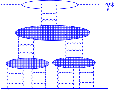
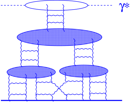
a)	b)

Figure 8: “Fan” diagrams (a) and $1/N_{c}$ corrections to them (b).

1992 - 1995  J.Bartels[16] showed that the non-linear equation can be correct only in large $N_{c}$ approximation since $1/N_{c}$ corrections (see Fig.  8-b ) lead to the interaction of two ladders in the “fan” diagrams (see also Ref. [17]. Laenen and Levin based on Ref.[18] generalized the non-linear equation, taking into account $1/N_{c}$ corrections in double log approximation [19]. It turns out that $1/N_{c}$-approximation works quite well in this problem and can be treated using the generating function formalism.

1994  L. McLerran and R. Venugopalan [5] noticed that at high density the gluonic fields are strong ( $G_{\mu\nu}\approx\,1/g$ where $\alpha_{s}=g^{2}/4\pi$) and, therefore, one can approach the high density QCD using the semiclassical gluon fields. Based on the space-time structure of the parton cascade at low $x$, they built the effective Lagrangian for high density QCD.

Figure 9: The space-time structure of the parton cascade at low $x$.

Indeed, the main and very important feature of the parton cascade, shown in Fig. 9, is the fact that a parton with higher energy in the cascade lives much longer than a parton with lower energy. We follow the parton emitted at time $t^{\prime}_{2}$. This parton lives a much shorter time than all partons emitted before. Therefore, all these partons will have enough time to form a current which depends on their density. Since the density is large we expect that the current is a classical current. Finally, the Lagrangian of the interaction for the parton emitted at time $t^{\prime}_{2}$ can be written as

$$L(\rho)\,\,+\,\,j_{\mu}\cdot A_{\mu}\,\,+\,\,L(A)\,\,,$$

where $A$ is the field of a parton emitted at $t^{\prime}_{2}$. However, we can consider a parton emitted at $t=t^{\prime}_{3}$ and include the previous one in the system with density $\rho$. The form of the Lagrangian should be the same. This is a strong condition (equation) on the form of the effective Lagrangian, so called Wilson renormalization group approach. This is the beautiful idea of the McLerran and Venugopalan which leads to Eq. 14, as we will show below.

1996  I. Balitsky [20] proved the non-linear equation in Wilson Loop Operator Expansion at high energies developed by him. Unfortunately, his paper was not noticed by the experts in the field including me. It should be stressed that he also gave an operator proof of the BFKL equation.

1997  Ayla, Ducati and Levin suggested non-linear equation [13] which differs from that of Eq. 14. They used the double log approximation but summed two DLA contributions

($(\alpha_{s}\ln(1/x)\ln(Q^{2}/\Lambda^{2}))^{n}$ and $(\alpha_{s}\ln(1/x)\ln(Q^{2}_{s}(x)/Q^{2}))^{n}$. It turns out that their equation is just the same equation as Eq. 14 but written for the opacity $\Omega$ instead of $N=(1-exp(-\frac{\Omega}{2}))$. AGL determined all numerical coefficients and discussed the initial condition of Eq. 14 which we will consider later.

1999 -2000  Yu. Kovchegov[21] proved Eq. 14 in the colour dipole approach [12]. It should be stressed that he not only gave the derivation which we have discussed, but he found a correct observable which enters the equation ($N$) and he suggested an initial condition that we will discuss below.

2000  M. Braun [22] calculated the “fan” diagrams of Fig. 8-a in the BFKl kinematic region, using the triple ladder vertex of Refs. [23].

2001  Iancu, A. Leonidov and L. McLerran [24] (see also Ref. [25]) proved Eq. 14 in the effective Lagrangian approach. Their proof is based on long and successive development of the effective Lagrangian approach exploited in Refs. [26]

3.3 Initial conditions:

One can see that Eq. 14 does not depend on the target and the dependence on the target comes from the initial conditions at some initial value of $x=x_{0}$. For a target nucleus it was argued [13, 21] that the initial conditions should be taken in the Glauber - Mueller form (see Eq. 5), namely,

$$N(x_{01},x=x_{0},b_{t})\,\,=\,\,N^{GM}(x_{01},x=x_{0},b_{t})=1\,\,-\,\,e^{-\,\frac{\Omega(x_{01},x=x_{0},b_{t})}{2}}\,\,.$$ (15)

The value of $x_{0}$ is chosen in the interval

$$e^{-\frac{1}{\alpha_{S}}}\,\leq\,x_{0}\,\leq\,\frac{1}{2\,m\,R}\,\,,$$

where $R$ is the radius of the target. In this region the value of $x_{0}$ is small enough to use the low $x$ approximation, but the production of the gluons (color dipoles) is still suppressed as $\alpha_{S}\ln(1/x)\,\leq\,\,1$. Therefore, in this region we have the instantaneous exchange of the classical gluon fields. Hence, an incoming color dipole interacts separately with each nucleon in a nucleus (see Ref. [27]).

For the hadron we have no proof that Glauber-Mueller formula is correct. As far as we understand the only criteria in this problem (at the moment) is the correct description of the experimental data. We described [28] almost all available HERA data using Eq. 5, and we feel confident using Eq. 5 as the initial condition for Eq. 14. It should be stressed that the experimental data on $dF_{2}/d\ln Q^{2}$ provides direct information on the integral over $b_{t}$ for $N$ since [29]

$$\frac{d\,F_{2}(x,Q^{2})}{d\ln Q^{2}}\,\,=\,\,\frac{Q^{2}}{3\pi^{3}}\,\,\int\,d^{2}\,b_{t}\,N(x,4/Q^{2},b_{t})\,\,+\,\,O(1/lnQ^{2})\,\,.$$ (16)

Choosing $x_{0}=10^{-2}$ we can make the initial condition practically independent of the parameterization of the $xG^{DGLAP}$ since all available parameterizations give the same prediction, even for the gluon density in this $x$ - range.

3.4 Theory status of the approach:

3.4.1 Parameters of the approach:

The master equation (Eq. 14) as well as the Glauber - Mueller formula (see Eq. 5 and Fig. 5 ) sums all diagrams of the order of

$$\left(\alpha^{2}_{S}\,(\frac{1}{x})^{\Delta}\,\right)^{n}\,\,\,{\rm with}\,\,\,\Delta\,\,\propto\,\,\alpha_{S}$$ (17)

It means that starting from $\alpha_{S}\ln(1/x)\,\,\approx\,\,\,\ln(1/\alpha_{S})$ the corrections related to the rescatterings of the partons and their interactions become essential. On the other hand, the next to leading order corrections to DGLAP or BFKL equations produce a value of $\Delta$ in Eq. 17 calculated up to $\alpha^{2}_{S}$ accuracy ( $\Delta=C_{1}\alpha_{S}+C_{2}\alpha^{2}_{S}$ ). Such corrections start to become important only for $\alpha_{S}\ln(1/x)\,\geq\,\,1/\alpha_{S}$ or , in other words, the next to leading order corrections have to be calculated after the rescatterings and parton interactions, included in the master equation, have been taken into account.

Therefore, the calculations of the next to leading order corrections for the linear evolution equations can be considered as a QCD motivated model in which crucial ad hoc assumptions have been made, namely, that the parton interactions and their rescatterings are small numerically.

3.4.2 Large $\mathbf{N_{c}}$ approach:

As has been discussed the master equation (Eq. 14) has only been proved in the large $N_{c}$ limit of QCD. The key question arises: could we develop a selfconsistent large $N_{c}$ approach for the DIS at low $x$. For $N_{c}\,\gg\,1$ we assume that $\hat{\alpha}_{S}\,\equiv\,\alpha_{S}\,N_{C}\,\,\approx\,1$ while $\alpha_{S}\,\ll\,1$, we assume all contributions that are proportional to $\alpha_{S}$ to be small so that we can neglect them. At first sight we have a problem with developing such an approach for high energy scattering. Indeed, the first Born diagram ( see Fig. 10 ) turns out to be of the order of $(N_{f}/N_{c})\hat{\alpha}^{2}_{S}$ where $N_{f}$ is the number of the quarks inside the proton. We can consider this parameter as being small in the large $N_{c}$ limit. However, it is well known that a nucleon consists of the $N_{c}$ ( $N_{f}=N_{c}$) number of quarks. This observation makes $(N_{f}/N_{c})\hat{\alpha}^{2}_{S}$ a ‘small parameter’ of the order of $\hat{\alpha}^{2}_{S}$.

Figure 10: The Borm approximation for the interaction of the virtual photon with the proton in large $N_{c}$ limit of perturbative QCD.

The amplitude $N({\mathbf{x_{01}}},b_{t}=0,y)\,\,\approx\,\,\hat{\alpha}^{2}_{S}/\pi R^{2}$ where $R$ is the radius of the proton for $N_{c}\,\gg\,1$. For large $N_{c}$ the interaction of two quarks is proportional to $\alpha_{S}$ and can be considered as small, but in the Hartree-Fock approximation it leads to a potential proportional to $\alpha_{S}\,N_{f}=\alpha_{S}\,N_{c}$. Therefore, $R\propto\hat{\alpha}_{S}$.

Finally, we conclude that the master equation sums all contributions of the order $\left(\hat{\alpha}_{S}\,\ln(1/x)\right)^{n}$ and gives a selfconsistent large $N_{c}$ limit for the DIS with the nucleons. In such an approach the DIS with mesons is suppressed by extra factor $1/N_{c}$. However, the equation itself depends only on $\hat{\alpha}_{S}$, and $1/N_{c}$ suppression for the mesons means that the initial condition could be written only as the first term of the Glauber-Mueller formula (see Eq. 5 ). Using this initial condition, we find the first $1/N_{c}$ corrections to the amplitude which will give the main contribution for the high energy ( low $x$ ) asymptotic.

It should be stressed that we still do not need to take $1/N_{c}$ corrections related to more complicated diagrams of the Fig. 8-b type into account. We would like to emphasize that the regular procedure, of how to calculate $1/N_{c}$ corrections, has been developed [19, 20, 25] and the first estimates have been made [19].

3.4.3 The region of applicability:

To evaluate the value of energy up to which we can use the master equation as a good theoretical tool for finding the high energy asymptotic, we need to estimate the contributions that have been neglected. We discuss all of them of the order of $1/N_{c}$, and they can be divided in two major classes:

• The first one is the interaction between two “ladders” of type Fig. 8-b . They are proportional to $\alpha_{S}/N^{2}_{c}\,\ln(1/x)$ [16], and therefore, we have a first restriction on the value of $x$:

  $$\frac{\hat{\alpha}_{S}}{N^{2}_{c}}\,\ln(1/x)\,\,<\,\,1\,\,\,{\rm or}\,\,\,\ln(1/x)\,\,<\,\,\frac{N^{2}_{c}}{\hat{\alpha}_{S}}\,\,;$$ (18)

• The second constraint comes from so called enhanced diagrams (see for an example Fig. 11 ).  The ratio of the contribution of this diagram to the “fan” diagram of Fig. 8-a is proportional to $\hat{\alpha}_{S}\,/N^{2}_{c}\,\ln(1/x)$ which leads to the same value at the highest energy, as does Eq. 18.

  Figure 11: The first enhanced diagram in the parton cascade.

Eq. 18 gives a sufficienly large value of energy upto which we can trust the master equation. The actual situation is much better. Indeed, the nonlinear equation leads to $N({\mathbf{x_{01}}},b_{t},y)\,\longrightarrow\,1$ at high energy, and we will argue below that this asymptotic limit will be reached at much lower energy than one defined by Eq. 18. Since $N({\mathbf{x_{01}}},b_{t},y)=1$ is the unitarity boundary for the scattering amplitude, the $1/N_{c}$ corrections cannot modify this result but could lead to a slightly different value of the saturation scale.

It should be stressed that the regular procedure of how to include $1/N_{c}$ corrections to the master equation, has been developed [19, 20, 24, 25] and even first estimates of the quantative effect of the $1/N_{c}$ corrections have been performed [19].

4 Saturation scale $\mathbf{Q_{s}(x)}$

4.1 Simple estimates:

The simplest estimates for the saturation scale come from the equation that the packing factor $\kappa$ is of the order of 1 [11, 13, 28]. Fig. 12 shows the solution of the equation

$$\kappa(x,Q^{2}_{s}(x))\,=\,1$$ (19)

As one can see $Q_{s}$ can be rather large even in HERA region. However, this estimate depends crucially on the value of $xG^{DGLAP}$.

Figure 12: The simplest estimate for the saturation scale $Q_{s}(x)$ from equation $\kappa(x,Q^{2}_{s}(x))\,=\,1,\,\,1.5\,\,0.5$.

4.2 Analytic solution of the non-linear equation:

Eq. 14 has been solved analytically with the simplified version of the BFKL kernel [30, 31, 25], namely, the Mellin transform $\chi(f)$ was taken as $\frac{1}{f}+\frac{1}{1-f}$ instead of $\chi(f)=2\psi(1)-\psi(f)-\psi(1-f)$, where $\psi$ is the derivative of the log of Euler gamma function. In terms of $s$-channel resummation Eq. 14 with this kernel sums two kinds of double logs: $(\alpha_{S}\ln(1/x)\,\ln(Q^{2}/\Lambda^{2}))^{n}$ for $Q^{2}>Q^{2}_{s}(x)$ and $(\alpha_{S}\ln(1/x)\,\ln(Q^{2}_{s}(x)/Q^{2}))^{n}$ for $Q^{2}<Q^{2}_{s}(x)$. For large $Q^{2}$ Eq. 14 can be reduced to the linear equation and can be solved using the trajectory (characteristics ) method [3, 32]. The structure of the trajectories both for linear and nonlinear equation is shown in Fig. 13.

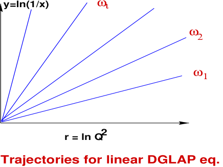
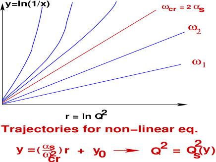
a)	b)

Figure 13: Trajectories for linear (a) and non-linear (b) equations.

The idea is to interpret the last linear trajectory ( line with $\omega_{cr}=2\,\alpha_{S}$ in Fig. 13-b ) of the linear equation which can be treated without nonlinear corrections, as the saturation scale. Doing so, we obtain [25, 30] the following expression for the saturation scale

$$Q^{2}_{s}(x)\,\,=\,\,Q^{2}_{s}(x=x_{0})\,\cdot\,\left(\,\frac{x_{0}}{x}\,\right)^{\frac{4N_{c}\alpha_{S}}{\pi}}$$ (20)

where $Q^{2}_{s}(x=x_{0}))$ is a saturation scale in our initial condition.

Therefore, we expect power-like rise of the saturation scale at low $x$.

4.3 Phenomenological saturation scale:

Golec-Biernat and Wuesthoff [33] suggested one could extract the value of $Q_{s}(x)$ from HERA data assuming that the saturation region has been reached at HERA. Surprisingly they managed to describe almost all HERA data using a simple parameterization for the saturation scale, namely,

$$Q^{2}_{s}(x)\,\,=\,\,(1\,\,GeV^{2})\,\cdot\,\left(\,\frac{x_{0}}{x}\,\right)^{\lambda}\,\,$$ (21)

with $\lambda=0.288$ and $x_{0}=3.04\times 10^{-4}$.

4.4 Saturation scale from numerical solution of the non-linear equation:

In Ref. [34] an attempt was made to solve the non-linear equation numerically (see also Ref. [22] ), starting from initial $x=x_{0}=10^{-2}$. Defining the saturation scale as a value of $r^{2}_{\perp}=4/Q^{2}_{s}(x)$ at which the imaginary part of the elastic amplitude for the dipole-target scattering is equal to 1/2

$$N(r_{\perp}=2/Q_{s},x)=\frac{1}{2}$$

the saturation scale shown in Fig. 14 was calculated.

Figure 14: The saturation scale $Q_{s}(x)$ plotted as a function of $lgx=log_{10}(x)$. GW denotes the saturation scale from Eq. 21

One can see that the saturation scale reaches a sufficiently large value of the order of $Q_{s}(x)\approx 14\,GeV$ at $x=10^{-7}$. It should be stressed that even at $x=10^{-5}$ which is in the typical range for THERA, the saturation scale is approximately 2 $\div$ 3 times larger than the Golec-Biernat and Wuesthoff estimates.

4.5 Saturation scale from DIS with nuclei:

The first estimates for the saturation scale in DIS on nuclei, presented in Fig. 15, shows that the nucleus target gives a promising avenue to increase the parton density without requiring a region of extremely low $x$. Comparing Fig. 15 with Fig. 14 we see that $Q_{s}(x)$ at $x=10^{-3}$ for gold is almost twice larger than for a nucleon.

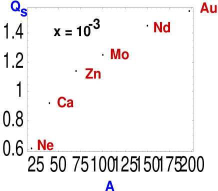
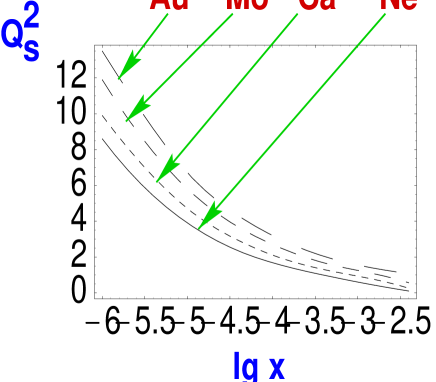
a)	b)

Figure 15: Saturation scale for DIS with nuclei: A (a) and $x$ (b) dependencies .

5 A new scaling in the saturation region.

The simple picture of the hadron in the saturation region shown in Fig. 1, leads to a new scaling phenomenon in this saturation region. We expect that the parton densities as well as cross sections are not functions of two variables:$x$ and $Q^{2}$, but they depend only on ratio $Q^{2}/Q^{2}_{s}(x)$ [3, 35, 5, 15, 30]. Stasto, Golec-Biernat and Kwiecinski [36] found that this scaling is valid for HERA data at $x<0.01$. Fig. 16 summarizes the situation and, here, I would like to comment on the theoretical arguments for such a new scaling scheme.

Figure 16:

5.1 Simple arguments for a new scaling:

Let us rewrite Eq. 14 in momentum space where it looks simpler

$$\frac{dN(Q,y,b_{t})}{dy}=\bar{\alpha}_{S}\left(\int K(Q,Q^{\prime})N(Q^{\prime},y;b_{t})-N^{2}(Q,y;b_{t})\right)\,\,.$$ (22)

For moments $N(\omega,Q)=N(\omega,Q_{0})\,e^{\gamma(\omega)\ln Q^{2}}$ Eq. 22 can be reduced to the form

$$\omega e^{\gamma(\omega)lnQ^{2}}=\chi(\gamma)e^{\gamma(\omega)lnQ^{2}}-N(\omega,Q_{0})\int d\omega^{\prime}e^{(\gamma(\omega^{\prime})+\gamma(\omega-\omega^{\prime})lnQ^{2}}$$ (23)

The integral over $\omega^{\prime}$ in Eq. 23 can be evaluated by saddle point method

$$\int d\omega^{\prime}e^{(\gamma(\omega^{\prime})+\gamma(\omega-\omega^{\prime})lnQ^{2}}\,\,\,\Longrightarrow\,\,\,e^{2\gamma(\omega/2)lnQ^{2}}$$

Therefore, we can see two different regions in the solution to Eq. 22: large $Q^{2}$, where the non-linear term is small and can be neglected, and low $Q^{2}$ where linear and nonlinear terms should be of the same order. It gives [35]

$$\gamma(\omega)=2\gamma(\omega/2)\,\,\quad\,\,\rightarrow\,\,\,\gamma(\omega)=C\omega$$ (24)

Using Eq. 24 we obtain for $N(y,Q^{2})$

$$N(y,Q^{2})=\int d\omega\,e^{-\omega y+\gamma(\omega)\ln Q^{2}}=\int d\omega e^{\omega(-y+C\ln Q^{2})}\,\,,$$ (25)

which means that $N(y,Q^{2})$ depends only on one variable [35]

$$-y+C\ln Q^{2}=\ln(Q^{2}_{s}(x)/Q^{2})=\xi\,\,.$$ (26)

It turns out that $C=\frac{\pi}{4N_{c}\alpha_{S}}$ in double log approximation [35, 25].

5.2 Scaling solution:

Eq. 26 gives the equation for the critical line $Q^{2}=Q^{2}_{s}(x)$ in Fig. 3.A more refined approach to the solution of the master non-linear equation, allows us to understand how far we have to move from the critical line to see this new scaling. It turns out that the scaling is not applicable [30] only in a narrow (at low $x$ ) band along the critical line with the width $\ln(Q^{2}_{s}(x)/Q^{2})\approx 1/4\alpha_{S}\,\ln(1/x)\,\ll\,1$ for $\alpha_{S}\,\ln(1/x)\,\gg\,1$.

It should be stressed that two quite different approaches: one is the analytic solution of the master equation [30] and the second is the solution of Wilson renormalization group equation for generating function [25], lead to the same answer and the same picture for the new scaling. The scaling solution is given in Fig.  17. the difference between $N(z,b_{t}=0)$ and $\sigma$ is due to the integration over impact parameter $b_{t}$.

a)	b)

Figure 17: (a) Dipole – target scattering amplitude $N(z)$ at $b_{t}=0$ and (b) dipole – target cross section $\hat{\sigma}(z^{\prime})$ in the scaling approximation versus scaling variable (a) $z=\ln(r^{2}_{\perp}\,Q^{2}_{s}(x))$ and (b) $z^{\prime}=\ln(Q^{2}_{s}(x)/Q^{2})$: Solid line is the scaling solution of the master equation, dashed line is a Golec-Biernat – Wusthoff model as explained in text and dotted line is the $z\gg 1$ asymptotic calculated in the first paper of Ref[30].

5.3 Scaling violation:

The question which we wish to address is how large is the scaling violation for $Q^{2}>Q^{2}_{s}(x)$. In Ref.[30] one can find first estimates of this scaling violation (see Fig. 18

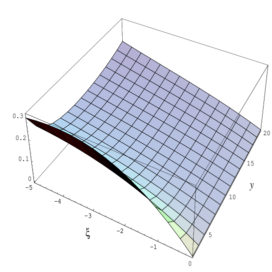
Figure 18: The ratio $\delta N(y,\xi)/N(\xi)$.

One can see that at all reasonable values of $y=\ln(1/x)$ and $\xi=\ln(Q^{2}_{s}(x)/Q^{2})$ the violation is less than 30$\%$. It means that if we want to have a tool to measure $Q^{2}_{s}(x)$ as a value of $Q^{2}$ at which we see a scaling violation, we have to establish a scale to an accuracy of less than 10$\%$. We think that it is instructive to examine Fig. 19 from this point of view. One can see from this figure that the accuracy of new scaling phenomena in HERA data is low, and we cannot use these data to measure the value of the saturation scale.

Figure 19: The HERA data, plotted as a function of $\tau=Q^{2}/Q^{2}_{s}(x)$. The solid curve is the prediction of the Wusthoff and Golec-Biernat saturation model, which was calculated by K. Golec-Biernat specially for THERA WS. The two dashed curves give the prediction of the DGLAP evolution (parameterization GRV’98) for the THERA kinematic region.

6 Parton densities at THERA and LHC energies

6.1 Analytic estimates:

All three theoretical analyses[6, 30, 25] of the master equation give the same result for the dipole-target amplitude $N(x,r_{\perp};b_{t})$, namely in the region of low $x$ $N(x,r_{\perp};b_{t})\,\longrightarrow\,1$ in accordance with the unitarity constraint. Eq. 12 leads to gluon structure function which can be calculated as follows

$$xG(x,Q^{2})\, = \,\frac{8}{\pi^{3}}\int^{1}_{x}\,\frac{dx^{\prime}}{x}\,\int^{\infty}_{4/Q^{2}}\,\frac{dr^{2}_{\perp}}{r^{4}_{\perp}}\,\int\,d^{2}\,b_{t}\,N(x^{\prime},r_{\perp};b_{t})$$ (27)

$$\longrightarrow \frac{2}{\pi^{2}}\,Q^{2}\,R^{2}\,\int^{y_{cr}}_{y}dy^{\prime}\,\,,$$

where $y_{cr}$ is the solution of the equation $Q^{2}_{s}(y_{cr})\,=\,Q^{2}$ and $R$ is the size of the target. Therefore, the answer for the asymptotic is clear, and it can be rewritten in the form [6, 30, 25]:

$$xG(x,Q^{2})\,\,\longrightarrow\,\,\frac{N^{2}_{c}-1}{4\pi N_{c}}\,\frac{1}{\alpha_{S}}\,\,R^{2}\,Q^{2}\,\ln(Q^{2}_{s}(x)/Q^{2})\,\,.$$ (28)

In Eq. 28 we assumed that the $b_{t}$ -distribution does not depend on $x$. Actually this is not correct and we have some shrinkage of the diffraction peak [30]. All numerical coefficients in Eq. 28 are fixed in the double log approximation and have to be checked to a better accuracy.

6.2 Numerical results:

The analytic approach leads to an understanding, but also gives a certain check of a numerical procedure for solving the master equation. At the moment, we have two attempts to solve the equation numerically [22, 34] which can illustrate the effect that the non-linear evolution will have for the extrapolation of HERA data to higher energies ( lower $x$). (see Fig. 20.

$\mathbf{x\,=\,10^{-7}}$	$\mathbf{x\,=\,10^{-6}}$
$\mathbf{x\,=\,10^{-4}}$	$\mathbf{x\,=\,10^{-3}}$

Figure 20: The comparison between the solutions $\tilde{N}$, Glauber-Mueller formula [28], and Golec-Biernat and Wuesthoff (GW) model. The four curves correspond to two different solutions $\tilde{N}_{\alpha_{S}=0.25}$ (large dashes), $\tilde{N}_{\alpha_{S}-running}$(small dashes), $N_{GM}$ (continuous line), and $N_{GW}$ of the GW model (dots).

We can learn at least two lessons: first, the approximate models cannot be used for the predictions at higher energies; and second, the saturation phenomenon could be rather strong both at THERA and LHC energies. Such a strong modification of the $r_{\perp}$ - behaviour due to non-linear corrections reflects in $Q^{2}$ and $x$ behaviour of gluon density as one can see in Fig.  21

Figure 21: The function $xG$ is plotted versus $\lg(x)$. The small dashes correspond to the solution with the running $\alpha_{S}$, while the large dashes are used for the constant $\alpha_{S}=0.25$. The continuous line is the GRV parameterization.

Fig. 21 shows that the taming of the parton densities growth included in the master equation can easily reduce the value of the gluon density at THERA and LHC energies by 2$\div$ 3 times, at different values of $Q^{2}$.

7 Summary

7.1 From the first principles:

The main message that I want to deliver in this presentation is very simple: Due to the hard work of number of experts, the theory of high parton density QCD has been established, and this theory includes the proof of :

• The nonlinear evolution equation for the dipole-target amplitude at fixed $b_{t}$ ($Im\,a(x,r_{\perp};b_{t})=N(x,r_{\perp};b_{t})$);

• The saturation of the parton densities as $x\rightarrow 0$ which means that $N(x,r_{\perp};b_{t})\,\longrightarrow\,1$ at low $x$;

• The new scaling phenomena $N(x,r_{\perp};b_{t})\,=\,N(r^{2}_{\perp}\cdot Q^{2}_{s}(x),b_{t})$ for $Q^{2}\,<Q^{2}_{s}(x)$;

• The sharp increase of the saturation scale $Q^{2}_{s}(x)$ in the region of low $x$;

• The importance of the saturation effects in taming the growth of the gluon density at THERA and LHC energies.

We would like to stress that during past two decades we have developed the perturbative QCD methods[21], based on the correct degrees of freedom: colour dipoles at high energies[11] and created new operator methods of tackling this problem, such as the Wilson Loop Operator Expansion[20] and the effective Lagrangian approach[5, 24, 25]. My personal feeling is that the future is in the operator methods since they provide a possibility to describe the matching of the high density QCD with real non-perturbative QCD with large coupling constant in a unique way. However, I would like to emphasize the positive aspects of the pQCD approach : a clear physical picture in the pQCD calculations and, because of this picture, the transparent understanding of the meanings of observables which we calculate in pQCD.

The whole development of this new area of theory I consider as a triumph of approach of my teacher, Prof. Gribov, to high energy physics, which could be formulated as “Physical picture - first, mathematics - after if ever”[38].   Indeed, I am very certain that the remarkable progress, that we see now, was possible only, because the picture that has been discussed in the first section, was correct from the beginning.

7.2 Our prejudices:

I decided to finish my paper listing the prejudices (some of them ) that I have fought during the two decades:

• The DGLAP evolution equation is more fundamental and has better proof than non-linear one. It is not true because

  • The GLAP equation yields the parton densities which violate the unitarity constraints;

  • The next to leading order corrections to the DGLAP evolution equation have to be included at energies $\ln(1/x)\,\geq 1/\alpha^{2}_{S}$ ( see section 3.4.1) which are much higher that the energy $\ln(1/x)\,\geq\ln(1/\alpha_{S})/\alpha_{S}$ when the parton rescatterings and recombinations start to be essential;

  • It does not contain any proof of why the higher twist contribution is smaller, than the leading twist one, which has been incorporated in these equations;

  • These equations demand initial conditions which we do not know how to treat theoretically or extract experimentally.

• By choosing the initial value for the DGLAP evolution $Q^{2}_{0}$ to be large enough, we can claim that the higher twists contributions are small. It was shown that the anomalous dimension of the higher twists is much larger that the leading one [16, 17] and at any value of $Q^{2}$ at low $x$, the higher twist will exceed the leading twist (DGLAP) contribution. Therefore, the practical procedure of solving the DGLAP evolution equation, cannot be considered to be free of justified criticism ;

• The calculation of higher order corrections of pQCD will improve our description of the experimental data. The pQCD series are the asymptotic series and they have intrinsic accuracy, which cannot be improved by calculating additional orders in $\alpha_{S}$, and this accuracy is rather poor in the region of low $x$. To evaluate errors we have to use the next order calculation in pQCD as an error, but with the same initial conditions.

7.3 The map of QCD

Figure 22: The map of QCD. $\alpha_{S}$ is the running QCD coupling constant, $\kappa=(3\pi^{2}\alpha_{S}/2Q^{2})\cdot(xG(x,Q^{2})/\pi R^{2})$ is the packing factor for the gluons. The saturation scale $Q^{2}=Q^{2}_{s}(x)$ is the line on which $\kappa=1$.

Fig. 22 displays the QCD map which is as the result of this approach. Three separate regions are distinguished by the size of the variables $Q^{2}$ and $x$. Each region corresponds to quit different physics.

1. Perturbative QCD domain where the constituents are of small size and their density is rather small so that we can neglect their interactions (recombinations). The packing factor $\kappa\,<1$ , and we can view this region as the traditional region for the linear QCD evolution equations ( the DGLAP and BFKL ones ). In this region the parton system appears as a Colour Dipole Gas, since we have here a rather dilute system of colour dipoles.

2. High parton density QCD domain in which the constituents are still small and we can use weak coupling methods, but their density is so large that the gluon field in this region becomes strong. We call the parton system in this domain a colour glass condensate[37], because gluons have colour, their fields evolve very slowly relative to the natural scale and are disordered. In simple words glass is a solid on a short time scale and a liquid on long time scale. In lectures by L. MacLerran [37]the reader can find the arguments why the parton system in this domain looks like a glass. We have a condensate because of high parton density and strong gluon fields in this region.

3. Non perturbative QCD domain in which the QCD coupling is large ($\alpha_{s}\,\,\approx\,\,1$). In this region the confinement of quarks and gluons occurs and a real non perturbative approach should be developed here. The key words for this domains are QCD vacuum, lattice QCD, effective Lagrangian approach, QCD - string theory duality and other lofty words about possible solutions of non perturbative QCD.

7.4 Acknowledgments :

I would like to thank all participants of low $x$ WG at THERA WS . Hot and useful discussions with them on high density QCD problems provided a stimulus for writing this presentation. I am very grateful for illuminating discussions to comrades in arms: Ian Balitsky,Jochen Bartels, Mikhail Braun, Asher Gotsman, Krystoff Golec-Biernat, Edmond Iancu, Dima Kharzeev, Boris Kopeliovich, Yura Kovchegov, Alex Kovner, Ian Kwiecinski, Uri Maor, Larry McLerran with his Minnesota-BNL team , Al Mueller and Heribert Weigert. I equally thank my students Mikhael Lublinsky,Eran Naftali and Kirill Tuchin for being good friends and labourers in the hard work on low $x$ problems.

I would also like to express a deep acknowledgment to my opponents for keeping me in a fighting mood. The present status of high density QCD is a challenge to them and , I hope, they will scrutinize and criticize our approach on the same professional level as it has been proven. I am sure that such a criticism will give a new impetus for further development.

I wish to thank all HERA experimentalists for their beautiful data and the deep interest in low $x$ problems. I have expressed my point of view on HERA data in different publication and, here, I wanted to give a review of the theoretical scene for them. I am very much indebted to them because HERA data revived a question on Pomeron structure , my first and strongest love which will never pass.

This research was supported in part by the BSF grant $\#$ 9800276, by the GIF grant $\#$ I-620-22.14/1999 and by Israeli Science Foundation, founded by the Israeli Academy of Science and Humanities.

References

-
[1]
V.N. Gribov and L.N. Lipatov,Sov. J. Nucl. Phys. 15 (1972) 438
;
L.N. Lipatov, Yad. Fiz. 20(1974) 181 ;
G. Altarelli and G. Parisi, Nucl. Phys. B126 (1977) 298;
Yu.L. Dokshitser, Sov. Phys. JETP 46(1977) 641. -
[2]
E.A. Kuraev, L.N. Lipatov and V.S. Fadin: Sov. Phys. JETP 45
(1978) 199;
Ya. Ya. Balitsky and L.N. Lipatov: Sov. J. Nucl. Phys. 28 (1978) 22. - [3] L.V. Gribov, E.M. Levin and M.G. Ryskin, Phys. Rep 100 (1983) 1; Nucl.Phys. B188 ((1981) 555.
- [4] A.H. Mueller and J. Qiu, Nucl. Phys. B268 (1986) 427.
- [5] L. McLerran and R. Venugopalan,Phys. Rev. D49 (1994) 2233,3352, 50 (1994) 2225, 53 (1996) 458, 59 (1999) 094002.
- [6] A.H. Mueller, Nucl. Phys. B558 (1999) 285.
-
[7]
R.P. Feyman, “ Photon - Hadron Interaction”, Benjamin, NY,1972;
J.D. Bjorken, J. Kogut and D.E. Soper, Phys. Rev. D3 (1971) 1382;
J.D. Bjorken, Phys. Rev. D1 (1970) 1376;
J.D. Bjorken and E. A. Paschos, Phys. Rev. 185 (1969) 1975. - [8] J. Bartels and H. Kowalski, “ Diffraction at HERA and the Confinement Problem”, DESY-00-154,hep-ph/0010345.
- [9] A. Zamolodchikov, B. Kopeliovich and L. Lapidus, JETP Lett. 33 (1981) 595;
- [10] E.M. Levin and M.G. Ryskin, Sov. J. Nucl. Phys. 45 (1987) 150.
- [11] A. H. Mueller, Nucl. Phys. B335 (1990) 115.
- [12] A.H. Mueller, Nucl. Phys. B415 (1994) 373.
- [13] A.L. Ayala, M.B. Gay Ducati and E.M. Levin, Nucl. Phys.B493(1997) 305, B511 (1998) 355;
-
[14]
N.N. Nikolaev and B.G. Zakharov, Z. Phys. C49 (1991) 607;
E.M. Levin, A.D. Martin, M.G. Ryskin and T. Teubner, Z. Phys. C74 (1997) 671. -
[15]
Yu. V. Kovchegov and L. McLerran, Phys. Rev. D60
(1999) 054025;
Yu. V. Kovchegov and E. Lervin, Nucl.Phys. B577 (2000) 221. - [16] J. Bartels, Z.Phys. C60 (1993) 471, Phys. Lett. B298 (1993) 204.
- [17] E.M. Levin, M.G. Ryskin and A.G. Shuvaev, Nucl. Phys. B387 (1992) 589.
- [18] E. Laenen,E. Levin and A.G. Shuvaev, Nucl. Phys. B419 (1994) 39.
- [19] E. Laenen and E. Levin, Nucl. Phys. (1995) 207; Ann.Rev.Nucl.Part.Sci. 44 (1994) 199-246.
- [20] I. Balitsky, Nucl. Phys. B463 (1996) 99, “High energy QCD and Wilson lines”, hep-ph/0101042 ,JLAB-THY-00-44.
- [21] Yu. V. Kovchegov, Phys. Rev. D60 (2000) 034008.
- [22] M. Braun, Eur. Phys.J. C16 (2000) 337.
-
[23]
A. Mueller and B. Patel, Nucl. Phys. B425 (1994) 471;
J. Bartels and M. Wuesthoff, Z. Phys. C66 (1995) 157. - [24] E. Iancu, A. Leonidov and L. McLerran, “Nonlinear Gluon Evolution in the Color Glass Condensate”, BNL-NT-00/24,hep-ph/0011241; “The renormalization group equation for the color glass condensate”, BNL-NT-01-3, hep-ph/0102009.
- [25] E. Iancu and L. McLerran, “ Saturation and Universality in QCD at small ”, SACLAY-T01-026, hep-ph/0103032.
-
[26]
J. Jalilian-Marian, A. Kovner, L. McLerran and H.
Weigert, Phys. Rev.D55(1997) 5414;
J. JuliLian-Marian, A. Kovner and H. Weigert, Phys. Rev. 59(1999) 014015;
J. Jalilian-Marian, A. Kovner, A. Leonidov and H. Weigert, Phys. Rev. 59(1999) 014014,034007,
A. Kovner, J.Guilherme Milhano and H. Weigert, Phys. Rev. D62(2000) 114005,
H. Weigert, “Unitarity at small Bjorken ” NORDITA-2000-34-HE, hep-ph/0004044. - [27] Yu. V. Kovchegov and A.H. Mueller, Nucl. Phys. B529 (1998) 451.
- [28] E. Gotsman et al. “Has HERA reached a new QCD regime?”, DESY-00-149, hep-ph/0010198.
- [29] A.L. Ayala, M.B. Gay Ducati and E.M. Levin, Phys. Lett. B388 (1996) 188.
- [30] E. Levin and K. Tuchin, Nucl. Phys. B573 (2000) 833; “ New scaling aty high energy DIS”, TAUP-2659-2000,hep-ph/0012167 ; Nonlinear evolution and saturation for heavy nuclei in DIS”, TAUP-2664-2001,hep-ph/0101275.
- [31] Yu.V. Kovchegov, Phys. Rev. D61 (2000) 074018.
-
[32]
J.C. Collins and J. Kwiecinski, Nucl. Phys. B335 (1990) 89;
J. Bartels, J. Blumlien and G. Shuler, Z. Phys. C50 (1991) 91. - [33] K. Golec-Biernat and M. Wuesthoff, “ Diffractive parton distributions from the saturation model”,DESY-00-180,hep-ph/0102093; Phys.Rev. D60 (1999) 114023;D59 (1999) 014017.
- [34] M. Lublinsky et al., “ Non-linear evolution and parton distributions at LHC and THERA energies”, TAUP-2667-2000,hep-ph/0102321.
- [35] J. Bartels and E. Levin, Nucl.Phys. B387 (1992) 617.
- [36] A. Stasto, K. Golec-Biernat and J. Kwiecinski, Phys.Rev.Lett. 86 (2001) 596.
- [37] L. McLerran, “ The Color Glass Condensate and Small Physics: 4 Lectures”, hep-ph/0104285.
- [38] Yu. Dokshitzer, “V.N. Gribov: 1930 -1997”, physics/9801025.