High-energy neutrinos and hard $\gamma$-rays
in coincidence with Gamma Ray Bursts

Abstract

The observations suggest that $\gamma$-ray bursts (GRBs) are produced by jets of relativistic cannonballs (CBs), emitted in supernova (SN) explosions. The CBs, reheated by their collision with the SN shell, emit radiation and Doppler-boost it to the few-hundred keV energy of the GRB’s photons. Chaperoning the GRB, there should be an intense flux of neutrinos of a few hundreds of GeV energy, made in $\pi^{\pm}$ decays: the SN shell acts as a dump of the beam of CBs. The $\nu$ beam carries almost all of the emitted energy, but is much narrower than the GRB beam and should only be detected in coincidence with the small fraction of GRBs whose CBs are very precisely pointing to us. The $\pi^{0}$s made in the transparent outskirts of the SN shell decay into energetic $\gamma$-rays (EGRs) of energy of ${\cal{O}}$(100) GeV. The EGR beam, whose energy fluence is comparable to that of the companion GRB, is as wide as the GRB beam and should be observable, in coincidence with GRBs, with existing or planned detectors.

Theory Division, CERN, Address
1211 Geneva 23, Switzerland
E-mail: alvaro.derujula@cern.ch

1 Introduction

For over thirty years, gamma ray bursts (GRBs) have been a great astrophysical mystery. Their origin is an unresolved enigma, in spite of recent remarkable observational progress: the discovery of GRB afterglows^?)?) the discovery^?) of the association of GRBs with supernovae (SNe), and the measurements of the redshifts^?) of their host galaxies. The current generally accepted view is that GRBs are due to synchrotron emission from fireballs produced by collapses or mergers of compact stars^?), by failed supernovae or collapsars^?), or by hypernova explosions^?). But various observations suggest that most GRBs are produced by highly collimated superluminal jets^?)?)?).

In a recent series of papers^?)?)?)?) Arnon Dar and I have outlined a cannonball (CB) model of GRBs which, we contend, is capable of describing the GRB phenomenology, and results in interesting predictions. For the sake of fairness and, speaking to an audience of particle physicists, I must admit that the reception of our CB model in the astrophysics community has, with a few significant exceptions, ranged from utter indiference to militant opposition. Arnon and I, who are optimists, consider this a very good omen, since in the ever evolving field of GRBs, and prior to every major shift in paradigm, the majority has always been wrong.

1.1 Interlude on the CB model

The CB model is based on the following analogies, hypothesis and explicit calculations:

Jets in astrophysics. Astrophysical systems, such as quasars and microquasars, in which periods of intense accretion into a massive object occur, emit highly collimated jets of plasma. The Lorentz factor $\rm\gamma\equiv 1/\sqrt{1-v^{2}/c^{2}}$ of these jets ranges from mildly relativistic: $\gamma\sim 2.55$ for PSR 1915+13^?), to quite relativistic: $\gamma={\cal{O}}\,(10)$ for typical quasars^?), and even to highly relativistic: $\gamma\sim 10^{3}$ for PKS 0405$-$385^?). These jets are not continuous streams of matter, but consist of individual blobs, or “cannonballs”. The jets emitted by quasars must be seen to be believed: they extend for many times the size of a galaxy, and they are unresolvably pencil-collimated till their material finally loses its kinetic energy to the intergalactic medium, stops and expands. The mechanism producing these surprisingly energetic and collimated emissions is not understood, but it seems to operate pervasively in nature (the mantra here is MHD, for magneto-hydrodynamics, which is not yet solved, particularly in its relativistic or general–relativistic versions.) We assume the CBs to be composed of ordinary “baryonic” matter (as opposed to $\rm e^{+}\,e^{-}$ pairs), as is the case in the microaquasar SS 433, from which Ly_α and metal K_α lines have been detected ^?)?).

The GRB/SN association. The original observation of an association between the exceptionally close-by GRB 980425 (redshift $\rm z=0.0085$) with the supernova SN 1998bw has developed into a convincing case for the claim^?) that many, perhaps all, of the long-duration GRBs are associated with SNe. Indeed, of the dozen and a half GRBs whose redshift is known, six or seven show in their afterglow a more or less significant additive “bump”, with the time dependence and spectrum of a SN akin to 1998bw^?), properly corrected^?) for the different redshift values. The example^?) of GRB 970228 is given in Fig.(1). In all the other cases^?) there is a good reason for such a bump not to have been seen, e.g. the afterglow itself is too luminous, as in the GRB 000301 example of Fig.(2); or the underlying galaxy is too luminous, as in the GRB 010222 example in the same figure, or the observations at the time the SN ought to be prominent are not available: the best reason not to have seen something. Thus, observationally, more than six out of sixteen —and perhaps all— of the GRBs of known redshift have a SN associated with them. The energy supply in a SN event similar to SN 1998bw is too small to accommodate the fluence of cosmological GRBs, unless their $\gamma$-rays are highly beamed. SN 1998bw is a peculiar supernova, but that may be due to its being observed close to the axis of its GRB emission. It is not out of the question that a good fraction –perhaps all– of the core-collapse SNe be associated with GRBs. To make the total cosmic rate of GRBs and SN compatible, this nearly one-to-one GRB/SN association would require beaming into a solid angle that is a fraction $\rm f\sim 2\times 10^{-6}$ of $4\pi$ ^?). The CB model, for the emission from CBs moving with $\gamma\sim 10^{3}$, implies precisely that beaming factor.

The GRB engine. We assume a core-collapse SN event not to result only in the formation of a central compact object and the expulsion of a supernova shell (SNS). A fraction of the parent star’s material, external to the newly-born compact object, should fall back in a time very roughly of the order of one day^?) and, given the considerable specific angular momentum of stars, it should settle into an accretion disk and/or torus around the compact object. The subsequent sudden episodes of accretion —occurring with a time sequence that we cannot predict— result in the emission of CBs. These emissions last till the reservoir of accreting matter is exhausted. The emitted CBs initially expand in the SN rest-system at a speed $\rm\beta\,c/\gamma$, with $\rm\beta\,c$ presumably of the same order or smaller than the speed of sound in a relativistic plasma ($\beta=1/\sqrt{3}$). The solid angle a CB subtends is so small that presumably successive CBs do not hit the same point of the outgoing SNS, as they catch up with it. These considerations are illustrated in Fig.(3).

The GRB. From this point onwards, the CB model is not based on analogies or assumptions, but on processes whose outcome can be approximately worked out in an explicit manner. The violent collision of the CB with the SNS heats the CB (which is not transparent at this point to $\gamma$’s from $\pi^{0}$ decays) to a temperature that, by the time the CB reaches the transparent outskirts of the SNS, is $\sim 150$ eV, further decreasing as the CB travels^?). The resulting CB surface radiation, Doppler-shifted in energy and forward-collimated by the CB’s fast motion, gives rise to an individual pulse in a GRB, as illustrated in Fig.(3). The GRB light curve is an ensemble of such pulses, often overlapping one another. The energies of the individual GRB $\gamma$-rays, as well as their typical total fluences, indicate CB Lorentz factors of ${\cal{O}}$(10³), as the SN/GRB association does^?). The observed fluence, light curves and energy spectra of GRBs are well described by the CB model^?).

The GRB’s afterglow. The CBs, after they exit the SNS, cool down by brems-strahlung and radiate by this process, by inverse Compton scattering, and by synchrotron radiation of their electrons on their enclosed magnetic field, much as the plasmoids emitted by quasars and microquasars do^?). The CB model provides an excellent detailed description of optical afterglows^?). The early afterglow spectrum and light curve are complicated by the fact that, about a day after the GRB emission, CBs cool down to a temperature at which $\rm e$–$\rm p$ recombination into $\rm H$ takes place. This gives rise to Ly-$\alpha$ lines that the CB’s motion Doppler-shifts to (cosmologically redshifted) energies of order a few keV, an energy domain that, interestingly, coincides with that of the $\rm Fe$ lines that an object at rest would emit. Recombination also gives rise to a multiband-flare in the afterglow. These CB-model’s expectations are in good agreement with incipient data on X-ray lines and flares^?), but the data are at the moment too scarce and imprecise to offer a decisive test of either the CB model or the Fe-line interpretation.

1.2 Back to introductory remarks

In this talk I concentrate on the $\nu$ and EGR signals that should occur in directional and temporal coincidence with GRBs. The neutrinos are made by the chain decays of charged pions, produced in the collisions of the CBs’ baryons with those of the SNS, as in Fig.(3). The $\nu$ beam carries almost all of the emitted energy, but is much narrower than the GRB beam and should only be detected in coincidence with the small fraction of GRBs whose CBs are moving extremely close to the line of sight. The EGRs are made by the decay of neutral pions, but only from $\pi^{0}$ production close enough to the outskirts of the SNS for the $\gamma$-rays not to be subsequently absorbed, see Fig.(3). The EGR beam, whose fluence is comparable to that of the GRB, is as wide as the GRB beam and should be observable, in coincidence with GRBs, with existing or planned detectors. The EGR beam peaks at energies of tens of GeVs, while the $\nu$ beam is about one order of magnitude more energetic.

In the space of a conference’s proceedings, I cannot detail the derivation of these results. In this written version I am mostly stating results, often in the form of commented figures.

2 Times and energies

To understand the CB model, one must keep four clocks simultaneously ticking on one’s head. Let $\rm\gamma=1/\sqrt{1-\beta^{2}}={E_{CB}/(M_{CB}c^{2})}$ be the Lorentz factor of a CB, which diminishes with time as the CB hits the SNS and as it subsequently plows through the interstellar medium. Let $\rm t_{SN}$ be the local time in the SN rest system, $\rm t_{CB}$ the time in the CB’s rest system, $\rm t_{Ob}$ the time measured by a nearby observer viewing the CB at an angle $\theta$ away from its direction of motion, and $\rm t$ the time measured by an earthly observer viewing the CB at the same angle, but from a “cosmological” distance (redshift $\rm z\neq 0$). Let x be the distance traveled by the CB in the SN rest system. The relations between the above quantities are:

$$\rm dt_{SN}=\gamma\,dt_{CB}=\rm{dx\over\beta\,c}\,;$$

$$\rm dt_{CB}\equiv\delta\,dt_{Ob}\,;$$

$$\rm dt=(1+z)\,dt_{Ob}={1+z\over\gamma\,\delta}\;dt_{SN}\;,$$ (1)

where the Doppler factor $\delta$ is:

$$\rm\delta\equiv\rm{1\over\gamma\,(1-\beta\cos\theta)}\simeq\rm{2\,\gamma\over(1+\theta^{2}\gamma^{2})}\;,$$ (2)

and its approximate expression is valid for $\theta\ll 1$ and $\gamma\gg 1$, the domain of interest.

Notice that for large $\gamma$ and not large $\theta\gamma$, there is an enormous “relativistic aberration”: $\rm dt\sim dt_{SN}/\gamma^{2}$, and the observer sees a long CB story as a film in extremely fast motion. As an example, consider a feature of a GRB light curve, such as a pulse of 2 s duration. Assume it is due to a GRB at $\rm z=1$, for which $\gamma=10^{3}$, and the viewing angle is $\theta=1/\gamma$. The duration of the pulse in the vicinity of the SN would be 1 s, corresponding to $10^{3}$ seconds in the CB system, and $10^{6}$ s (11.6 days) of travel of the CB through interstellar space. Everything that happens to the CB in its journey of a dozen light-days, the observer sees in 2 seconds!

The energy of the photons radiated by a CB in its rest system, $\rm E^{\gamma}_{CB}$, their energy in the direction $\theta$ in the local SN system, $\rm E^{\gamma}_{SN}$, and the photon energy $\rm E$ measured by a cosmologically distant observer, are related by:

$$\rm E^{\gamma}_{CB}={E^{\gamma}_{SN}\over\delta}\,;\;\;\;\;\;E^{\gamma}_{SN}=(1+z)\,E\;,$$ (3)

with $\delta$ as in Eq.(2). Relative to their energy at the SN location, the GRB’s photons are blue-shifted by a factor $\delta$ and red-shifted by $\rm 1+z$. This brings the photon energy of the CB’s surface radiation to the observed GRB domain.

3 Reference values of various parameters

To be explicit we must scale our results to given values of the parameters of the CB model, which serve as benchmarks but imply no strong commitment to their particular choices. These values are listed in Table I, for quick reference.

Parameter	Symbol	Value
SN-shell’s mass	$\rm M_{S}$	$\rm 10\;M_{\odot}$
SN-shell’s radius	$\rm R_{S}$	$2.6\times 10^{14}$ cm
Outgoing Lorentz factor	$\rm\gamma_{out}$	$10^{3}$
CB’s energy	$\rm E_{CB}$	$10^{52}$ erg
Initial $\rm v_{{}_{T}}/c$ of expansion	$\rm\beta_{in}$	$1/(3\,\sqrt{3})$
Final $\rm v_{{}_{T}}/c$ of expansion	$\rm\beta_{out}$	$1/\sqrt{3}$
Redshift	z	1
CB’s viewing angle	$\theta$	$\rm 10^{-3}$

Table 1: List of the “reference” values of various parameters. $\rm z$ and $\theta$ are not specific to the model.

Let “jet” stand for the ensemble of CBs emitted in one direction in a SN event. If a momentum imbalance between the opposite-direction jets is responsible for the large peculiar velocities of neutron stars^?), ${\rm v_{NS}\approx 450\pm 90~{}km~{}s^{-1}}$, the jet kinetic energy $\rm E_{jet}$ must be, as we shall assume for our GRB engine, larger than^?) $\rm M_{NS}\,v_{NS}\,c\sim 10^{52}$ erg, for $\rm M_{NS}=1.4\,M_{\odot}$. We adopt a value of $10^{53}$ ergs as the reference jet energy. On average, GRBs have some five to ten significant pulses, so that the energy in a single CB may be 1/5 or 1/10 of $\rm E_{jet}$. We adopt $\rm E_{CB}=10^{52}$ erg as our reference.

Let $\rm\gamma_{in}$ be the Lorentz factor of a cannonball as it is fired. We find $\rm\gamma_{in}={\cal{O}}(3\times 10^{3})$ to be a “typical” value ($\rm\gamma_{in}$ is not an “input” parameter). For this value and the reference CB energy, the CB’s mass is very small by stellar standards, and comparable to an Earth mass: $\rm M_{CB}\sim 0.6\,M_{\otimes}\;{(3\times 10^{3})/\gamma_{in}}$. The baryonic number of the CB is:

$$\rm N_{b}\simeq{E_{CB}\over m_{p}\,c^{2}\,\gamma_{in}}\simeq 2.2\times 10^{51}\;{{E}_{CB}\over 10^{52}\;erg}\,\left[{3\times 10^{3}\over\gamma_{in}}\right].$$ (4)

Thus, the CB accelerator is comparable to the Tevatron in energy per proton ($\rm E_{p}={\cal{O}}(1)$ TeV), but it has a better flux ($10^{51}$ p.p.p.) The trouble is that nobody has a convincing idea about how the accelerating trick is played.

We have assumed that, in a SN explosion, some of the material outside the collapsing core is not expelled as a SNS, but falls back onto the compact object. For vanishing angular momentum, the free-fall time of a test-particle from a distance $\rm R$ onto an object of mass ${\rm M}$ is $\rm t_{fall}=\pi\,[R^{3}/(8\,G\,M)]^{1/2}$. For material falling from a typical star radius ($\rm R_{\star}\sim 10^{12}$ cm) on an object of mass $\rm M=1.4\;M_{\odot}$, $\rm t_{fall}\simeq 1$ day. The fall-time is longer (except for material falling from the polar directions) if the specific angular momentum is considerably large, as it is in most stars. The fall-time is shorter for material not falling from as far as the star’s radius. The estimate $\rm t_{fall}\simeq 1$ day is therefore a very rough one. One day after core-collapse, the expelled SNS, travelling at a velocity^?) $\rm v_{S}\sim c/10$, has moved to a distance of $\rm R_{S}=2.6\times 10^{14}$ cm, which we adopt as our reference value.

For the Lorentz factor of the CBs as they exit the SNS, we adopt the value $\rm\gamma_{out}=10^{3}$, for the reasons discussed in the Introduction. Let $\rm\beta_{in}\,c$ be the expansion velocity of a CB, in its rest system, as it travels from the point of emission to the point at which it reaches the SNS, and let $\rm\beta_{out}\,c$ be the corresponding value after the CB exits the SNS, reheated by the collision. We expect these velocities to be comparable to the speed of sound in a relativistic plasma, $\rm c/\sqrt{3}$, as observed in the initial expansion of the CBs emitted by GRS 1915+13^?). As reference values, we adopt those of Table I.

4 A cannonball’s collision with a supernova shell

The density profile of the material in a SNS (as a function of distance $\rm x$ to the SN centre) is observationally known, at least for the outer transparent regions of the shell^?). It is roughly given as a power law $\rm\rho\propto x^{-n}$, with $\rm n=4$ to 8. Given the assumed properties of our CBs, we can approximately figure out what happens in their collision with a SNS of given mass, radius and density index $\rm n$.

The CB and the SNS are sufficiently thin for the charged pions produced in $\rm pp$ (or nucleon-nucleon) collisions and the subsequent muons to decay: about two thirds of the original energy of a colliding CB’s nucleon results in $\nu$ production. The CB and the SNS are sufficiently thick for all incoming nucleons to interact. The CB’s energy is much bigger than the “target” rest energy of the material removed from the “bullet-hole” which the CB makes in the SNS. It follows from all this that the relation between the Lorentz factors of the CB before and after it crosses the SNS, is:

$$\rm\gamma_{out}\simeq\gamma_{in}\;\sqrt{2\,E_{CB}\over 3\,\beta_{in}^{2}\,M_{S}\,c^{2}+18\,E_{CB}}\,.$$ (5)

For large $\rm E_{CB}$, $\rm\gamma_{in}\sim 3\,\gamma_{out}$, while for our reference parameter values $\rm\gamma_{in}\sim 10\,\gamma_{out}$: the model requires values of $\rm\gamma_{in}$ as surprisingly large as $10^{4}$.

After the CB and the target SNS material collide and coalesce, all nucleons of the CB must have slowed down from $\rm\gamma_{in}$ to $\rm\gamma_{out}$, which takes a few collisions of high c.m.s. energy. The neutrinos made in these collisions escape. I shall outline how this allows us to estimate the $\nu_{\mu}$ flux as a function of energy and production angle explicitly, by use of the empirical knowledge on pion and “leading particle” production in nucleon-nucleon collisions.

One can similarly estimate the EGR flux. The CB-SNS collision results in the production of $\pi^{0}$s. The energetic $\gamma$ rays from $\pi^{0}\rightarrow\gamma\gamma$ decay, of energy a few hundred GeV, can only escape from the transparent outskirts of the SNS, of grammage $\rm X_{EGR}\sim 70$ g/cm²: their observable flux is much smaller than that of neutrinos. The number of “target” SNS nucleons involved in the production of escaping EGRs is:

$$\rm N_{p}^{EGR}\approx\pi\;\widetilde{R}_{CB}^{2}\,{X_{EGR}\over m_{p}}\simeq 1.4\times 10^{49}\;,$$ (6)

where $\rm\widetilde{R}_{CB}$ the radius of the CB as it reaches the transparent outer shell. The numerical value is for our reference parameters (the general expression^?) for $\rm N_{p}^{EGR}$ is complicated).

In the CB model the GRB $\gamma$ rays, of much lower energy than the EGRs, result from the quasi-thermal emission from the CB’s front-surface, heated by the collision with the SNS. Their detailed discussion is elaborate^?). For our reference parameters, the total GRB energy in the CB rest system is $\rm E_{pulse}^{rest}\sim 3\times 10^{45}$ erg. An observer at rest, located at a known luminosity distance $\rm D_{L}(z)$ from the CB and viewing it at an angle $\theta$ from its direction of motion, would measure a “total” (time- and energy-integrated) fluence per unit area:

$$\rm{df\over d\Omega}\simeq{1+z\over 4\,\pi\,D_{L}^{2}}\,{E_{pulse}^{rest}}\;\left[{2\,\gamma_{out}\over 1+\theta^{2}\,\gamma_{out}^{2}}\right]^{3}\;.$$ (7)

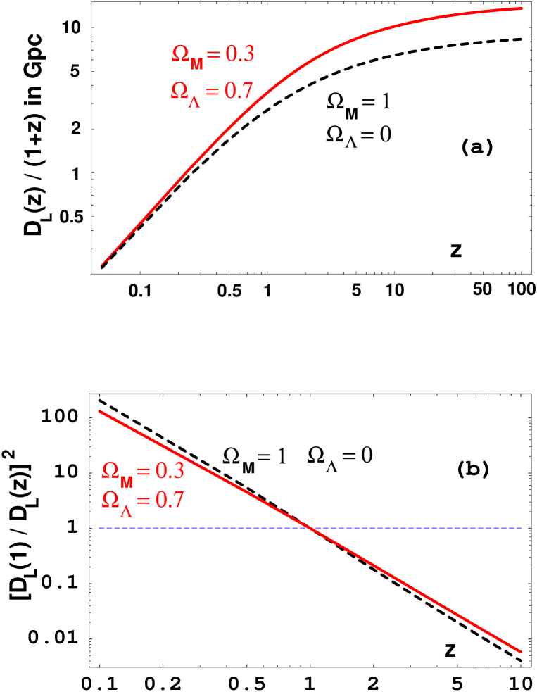
Figure 4: Luminosity distances and ratios thereof, as functions of redshift, for two $\Omega=1$ Friedman universes, with two choices of matter and vacuum densities.

Of the three powers of $\delta$, the Doppler factor of Eq.(2), one reflects the energy boost, and two the narrowing of the (solid) angle. The photons in the GRB are beamed in a cone of aperture $\rm 1/\gamma_{out}$. In our explicit calculations, and in the conventional cosmological notation, we use $\rm H_{0}=65$ km/(s Mpc), ${\rm\Omega_{M}}=0.3$ and ${\rm\Omega_{\Lambda}}=0.7$, so that, for example, $\rm D_{L}(1)\simeq 7.12$ Gpc $\simeq 2.20\times 10^{28}$ cm. In Fig.(4) I show $\rm D_{L}(z)$ and $\rm[D_{L}(1)/D_{L}(z)]^{2}$ (the quantity to which we shall scale our results) for the quoted cosmology and, for comparison, for the case $\rm\Omega_{M}=1$, $\rm\Omega_{\Lambda}=0$. At moderate $\rm z$, the results are not very sensitive to the choice of cosmological parameters.

5 The flux of EGRs

The approximate isospin independence of nuclear interactions implies that, in the high energy collisions of protons or neutrons on protons or neutrons, the production of $\pi^{+}$, $\pi^{0}$ and $\pi^{-}$ is similar. To compute the spectrum of outgoing photons per nucleon–nucleon collision, we convolute the observed distribution of $\pi^{\pm}$s (assumed to describe $\pi^{0}$ production as well) with the $\gamma$ distribution in $\pi^{0}$ decay. The resulting distribution in $\rm y\equiv E_{\gamma}/E_{p}$ and $\gamma$ transverse momentum $\rm p_{T}$, can be fitted by:

$$\rm{1\over\sigma_{pp}^{TOT}}\,{d\sigma^{\gamma}\over dp_{{}_{T}}^{2}\,dy} \simeq \rm\rm A_{\gamma}\,{1\over y}\,e^{-b_{\gamma}y}\;{1\over 2\,\bar{p}_{T}^{2}}\,e^{-p_{{}_{T}}/\bar{p}_{{}_{T}}}\;,$$

$$\rm A_{\gamma} \simeq \rm 1.1\;,\;\;\;b_{\gamma}\simeq 8\,,\;\;\;\;\bar{p}_{{}_{T}}\sim 160~{}MeV\,.$$ (8)

An exponential fit in $\rm y$ is inadequate close to the limit $\rm y=1$, but for $\rm y>1/2$ the flux is negligible. The advantage of our simple fits is that they allow us to give analytical estimates all the way to the observable particle fluxes.

Let $\rm E_{\gamma}$ be the energy of a photon as it reaches the Earth, cosmologically red-shifted by a factor $\rm 1+z$, and let $\rm E_{p}\simeq m_{p}\,c^{2}\,\gamma_{out}$ be the energy of the CB’s nucleons, in the local rest system of their SN progenitor, as they reach the outer part of the SNS. For the small angles $\theta$ at which the $\gamma$-rays are forward-collimated by the relativistic motion of the parent $\pi^{0}$’s, the photon-number distribution in $\rm x_{\gamma}=E_{\gamma}/E_{p}$ and $\cos\theta$, per single nucleon–nucleon collision, is:

$$\rm{dn_{\gamma}\over dx_{\gamma}\;d\cos\theta} \simeq \rm B_{\gamma}\;(1+z)^{2}\;x_{\gamma}\;e^{-c_{\gamma}\,x_{\gamma}}$$

$$\rm B_{\gamma} \simeq \rm A_{\gamma}\;\left[{m_{p}\,c\,\gamma_{out}\over\bar{p}_{{}_{T}}^{\gamma}}\right]^{2}\simeq(3.76\times 10^{7})\,\left[{\gamma_{out}\over 10^{3}}\right]^{2}$$

$$\rm c_{\gamma} = \rm c_{\gamma}(z,\theta,\gamma_{out})\simeq\rm(1+z)\,\left[b_{\gamma}+{m_{p}\,c\,\gamma_{out}\,\theta\over\bar{p}_{{}_{T}}^{\gamma}}\right]\,.$$ (9)

Let $\rm dn_{\gamma}/d\Omega$ be the total (time-integrated) number flux of EGR photons per unit solid angle about the direction $\theta$ (relative to the CBs’ direction of motion) at which they are viewed from Earth. The photon number distribution per incident CB is:

$$\rm{dn_{\gamma}\over dx_{\gamma}\,d\Omega} \sim \rm{N_{p}^{EGR}\,B_{\gamma}\over 2\,\pi\;D_{L}^{2}}\;(1+z)^{4}\;f_{\gamma}$$

$$\rm f_{\gamma} \equiv \rm f_{\gamma}(z,\gamma_{out},\theta,x_{\gamma})\simeq x_{\gamma}\;e^{-c_{\gamma}\,x_{\gamma}}\;,$$ (10)

with $\rm N_{p}^{EGR}$ given by Eq.(6). Since a typical GRB has an average of $\rm n_{CB}=5$ to 10 significant pulses, the total flux of EGRs in coincidence with a GRB may be an order of magnitude above that of Eq.(10). In Fig.(5a) we show $\rm f_{\gamma}$ as a function of $\rm x_{\gamma}$ at various $\theta$; for $\rm z=1$ and $\rm\gamma_{out}=10^{3}$. The average fractional EGR energy in the spectrum of Eq.(10) is $\rm\bar{x}_{\gamma}=2/c_{\gamma}$, corresponding, at $\rm z=1$ and for $\rm\gamma_{out}=10^{3}$, to average energies $\rm\bar{E}_{\gamma}\sim 120$ GeV for $\theta=0$, $\rm\bar{E}_{\gamma}\sim 70$ GeV for $\rm\theta=1/\gamma_{out}$, and $\rm\bar{E}_{\gamma}\sim 40$ GeV for $\rm\theta=3/\gamma_{out}$, a more probable angle of detection^?). Except at the highest of these energies and/or at redshifts well above unity, the absorption of $\gamma$-rays on the infrared background —for which we have not corrected Eq.(10)— is negligible.

Roughly characterize the efficiency of a $\gamma$-ray detector as a step function $\rm\Theta(E^{\gamma}-E^{\gamma}_{min})$. The total flux above threshold, per incident CB, is then:

$$\rm{dn^{T}_{\gamma}[x^{\gamma}_{min},\theta]\over d\Omega} \sim \rm{dn^{T}_{\gamma}[0,0]\over d\Omega}\;G_{\gamma}(z,\gamma_{out},\theta,x^{\gamma}_{min})$$

$$\rm G_{\gamma} \simeq \rm\left[{(1+z)\,b_{\gamma}\over c_{\gamma}}\right]^{2}\,(1+c_{\gamma}\,x^{\gamma}_{min})\,e^{-c_{\gamma}\,x^{\gamma}_{min}}$$

$$\rm x^{\gamma}_{min} \equiv \rm{E^{\gamma}_{min}\over m_{p}\,\gamma_{out}}$$

$$\rm{dn^{T}_{\gamma}[0,0]\over d\Omega} \simeq \rm{1.1\times 10^{8}\over km^{2}}\,{N_{p}^{EGR}\over 1.4\;10^{49}}\,\left[{\gamma_{out}\over 10^{3}}\right]^{2}\left[{1+z\over 2}\right]^{2}\,\left[{D_{L}(1)\over D_{L}(z)}\right]^{2}\,.$$ (11)

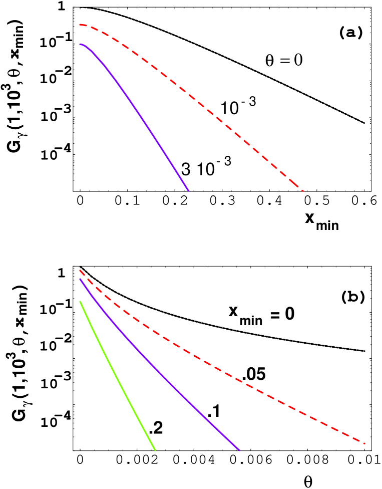
Figure 6: The function $\rm G_{\gamma}$ of Eq.(11), for $\rm z=1$ and $\rm\gamma_{out}=10^{3}$. Top: As a function of $\rm x_{min}$ at various fixed $\theta$. Bottom: vice versa.

In Fig.(6a) and (6b) we show $\rm G_{\gamma}$ as a function of $\rm x^{\gamma}_{min}$ at various fixed $\theta$, and vice versa; for $\rm z=1$ and $\rm\gamma_{out}=10^{3}$. The very large flux $\rm dn^{T}_{\gamma}[0,0]/d\Omega$ of Eq.(11) is seen to be significantly reduced as soon as $\theta$ and/or $\rm x^{\gamma}_{min}$ depart from zero: the EGR flux is not as gigantic as it appears to be at first sight.

6 The flux of high energy neutrinos

The calculation of the $\nu_{\mu}$ flux produced in the collision of a CB with the SNS is analogous to the calculation of the EGR photon flux. The $\bar{\nu}_{\mu}$ flux gives rise to a signal of about 1/3 the size of that of the $\nu_{\mu}$ flux (we neglect it, since we find it preferable to establish a lower limit to the observational prospects). The $\nu_{\mu}$’s are made in the chain reactions $\rm p\,p\to\pi+...$, $\pi^{+}\to\mu^{+}\,\nu_{\mu}$; and $\pi^{-}\to\mu^{-}\,\bar{\nu}_{\mu}$, followed by $\mu^{-}\to e^{-}\,\nu_{\mu}\,\bar{\nu}_{e}$. The contribution of $\rm K$ production and decay turns out to be negligible.

The calculation of the $\nu_{\mu}$ flux is akin to that of the EGR flux. Absorption in the SNS no longer plays a role, and $\nu$s are produced by the collisions of all the nucleons in the CB as they suffer a few high c.m.s. energy collisions to slow down from $\rm\gamma_{in}$ to $\rm\gamma_{out}$. The result of our analysis is a distribution in $\rm y=E_{\nu}/E_{p}$ (with $\rm E_{p}$ the incoming nucleon’s energy) and $\rm p_{T}^{\nu}$, which is of the same from as Eq.(8), but for which

$$\rm A_{\nu}\simeq\rm 3\;,\;\;\;b_{\nu}\simeq 12\,,\;\;\;\;\bar{p}_{T}^{\nu}\sim 190~{}MeV\,.$$ (12)

Let $\rm E_{\nu}$ be the redshifted energy of a neutrino as it reaches the Earth, and let $\rm E_{p}\simeq m_{p}\,c^{2}\,\gamma_{in}$ be the energy of the CB’s nucleons, in the local rest system of their SN progenitor, as they enter the SNS. In analogy with Eq.(9) the $\nu_{\mu}$-number distribution in $\rm x_{\nu}=E_{\nu}/E_{p}$ and $\cos\theta$, per single nucleon–nucleon collision, is:

$$\rm{dn_{\nu}\over dx_{\nu}\;d\cos\theta} \simeq \rm B_{\nu}\;(1+z)^{2}\;x_{\nu}\;e^{-c_{\nu}\,x_{\nu}}$$

$$\rm B_{\nu} \simeq \rm A_{\nu}\;\left[{m_{p}\,c\,\gamma_{in}\over\bar{p}_{{}_{T}}^{\nu}}\right]^{2}\simeq(6.0\times 10^{7})\,\left[{\gamma_{in}\over 10^{4}}\right]^{2}$$

$$\rm c_{\nu} = \rm c_{\nu}(z,\theta,\gamma_{in})\simeq(1+z)\,\left[b_{\nu}+{m_{p}\,c\,\gamma_{in}\,\theta\over\bar{p}_{{}_{T}}^{\nu}}\right]\,.$$ (13)

Notice that the above equations contain $\rm\gamma_{in}$, and not $\rm\gamma_{out}$, as the analogous ones for EGRs did. If you have not understood this, I have lost you already. Let $\rm dn_{\nu}/d\Omega$ be the time-integrated number of neutrinos per unit solid angle about the direction $\theta$ (relative to the CBs’ direction of motion) at which they are viewed from Earth. In analogy with Eq.(10), the neutrino number distribution, per incident CB, is:

$$\rm{dn_{\nu}\over dx_{\nu}\,d\Omega} = \rm{N_{b}\,B_{\nu}\over 2\,\pi\;D_{L}^{2}}\;(1+z)^{4}\;f_{\nu}$$

$$\rm f_{\nu} = \rm f_{\nu}(z,\gamma_{in},\theta,x_{\nu})\simeq x_{\nu}\;e^{-c_{\nu}\,x_{\nu}}\;,$$ (14)

with $\rm N_{b}$ the CB’s baryon number, given by Eq.(4). For a GRB with $\rm n_{CB}$ significant pulses, the total number of neutrinos is $\rm n_{CB}$ times larger than that of Eq.(14).

In Fig.(5b) we show $\rm f_{\nu}$ as a function of $\rm x_{\nu}$ at various $\theta$; for $\rm z=1$ and $\rm\gamma_{in}=10^{4}$. The average fractional $\nu$ energy in the spectrum of Eq.(14) is $\rm\bar{x}_{\nu}=2/c_{\nu}$, corresponding, for the chosen $\rm z$ and $\rm\gamma_{in}$, to average energies $\rm\bar{E}_{\nu}\sim 712$ GeV for $\theta=0$, $\rm\bar{E}_{\nu}\sim 315$ GeV for $\rm\theta=1/10^{3}$, and $\rm\bar{E}_{\nu}\sim 150$ GeV for $\rm\theta=3/10^{3}$.

Neutrino oscillations may reduce the flux of $\nu_{\mu}$s of Eq.(14) by as much as a factor of 2 (if they are maximal) or even 3 (if they are “bimaximal”).

6.1 Muon production on Earth

Muon neutrinos produced by a GRB can be detected by large-area or large-volume detectors, in temporal and directional coincidence with a GRB $\gamma$-ray signal. The detection technique typically involves the “upward-going” muons, for which there is no “atmospheric” cosmic-ray background. To compute the number of muons of a fixed energy observable per unit area, one must solve the quasi-equilibrium equation describing the competing processes of muon production and muon energy-loss. At the relatively low energies of interest here, the details pile up into a single prefactor:

$$\rm\rm K\simeq\rm\rho_{W}\,N_{A}\,{1\over R_{0}}\,{\sigma_{{}_{CC}}\over E_{\nu}}\simeq 2.26\times 10^{-12}\;GeV^{-2}\;,$$ (15)

where $\rm\rho_{W}$ is the density of water, $\rm N_{A}$ is Avogadro’s number, $\rm R_{0}$ is an energy loss of 2.12 MeV/cm and $\rm\sigma_{CC}/E_{\nu}\sim 0.8\;10^{-38}$ cm²/GeV is the slope of the charged current $\nu_{\mu}$ cross section on an isoscalar nucleon.

Define $\rm x_{\mu}=E_{\mu}/E_{p}$: the ratio of the energy of a muon produced on Earth to the energy $\rm E_{p}=m_{p}\,c^{2}\,\gamma_{in}$ of the CB’s nucleons, as they enter the SNS. We obtain a muon flux per incident CB:

$$\rm{dn_{\mu}\over dx_{\mu}\,d\Omega} \sim \rm K\,E_{p}^{2}\,{N_{b}\,B_{\nu}\over 2\,\pi\,D_{L}^{2}}\;(1+z)^{4}\;f_{\mu}(z,\gamma_{in},\theta,x_{\nu})$$

$$\rm f_{\mu} = \rm\;{2+c_{\nu}\,x_{\mu}\over c_{\nu}^{3}}\;e^{-c_{\nu}\,x_{\mu}}\,,$$ (16)

with $\rm B_{\nu}$ and $\rm c_{\nu}$ as in Eq.(13) and $\rm N_{b}$ the total baryon number of the CB, Eq.(4). In Fig.(5c) we show $\rm f_{\mu}$ as a function of $\rm x_{\mu}$ at various $\theta$, for $\rm z=1$ and $\rm\gamma_{in}=10^{4}$.

Very roughly characterize the efficiency of an experiment as a step function jumping from zero to unity at $\rm E^{\mu}=E^{\mu}_{min}$. The observable number of muons per CB and per unit area, obtained by integration of Eq.(16), then is:

$$\rm{dn^{T}_{\mu}[x^{\mu}_{min},\theta]\over d\Omega} \sim \rm{dn^{T}_{\mu}[0,0]\over d\Omega}\;G_{\mu}(z,\gamma_{in},\theta,x^{\mu}_{min})$$

$$\rm G_{\mu} = \rm\left[{(1+z)\,b_{\nu}\over c_{\nu}}\right]^{4}\;\left(1+{c_{\nu}\,x^{\mu}_{min}\over 3}\right)\;e^{-c_{\nu}\,x^{\mu}_{min}}$$

$$\rm x^{\mu}_{min} \equiv \rm{E^{\mu}_{min}\over m_{p}\,\gamma_{in}}$$

$$\rm{dn^{T}_{\mu}[0,0]\over d\Omega} \simeq \rm{3.2\times 10^{2}\over km^{2}}\,{E_{CB}\over 10^{52}\;erg}\,\left[{\gamma_{in}\over 10^{4}}\right]^{3}\,\left[{D_{L}(1)\over D_{L}(z)}\right]^{2}\,.$$ (17)

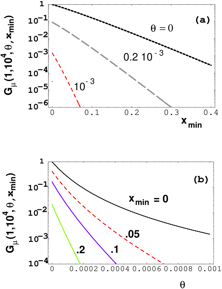
Figure 7: The function $\rm G_{\mu}$ of Eq.(17), for $\rm z=1$ and $\rm\gamma_{in}=10^{4}$. Top: As a function of $\rm x_{min}$ at various fixed $\theta$. Bottom: vice versa.

In Figs.(7a,b) we show $\rm G_{\mu}$ as a function of $\rm x^{\mu}_{min}$ at various fixed $\theta$, and vice versa; for $\rm z=1$ and $\rm\gamma_{in}=10^{4}$. The relatively large flux $\rm dn^{T}_{\mu}[0,0]/d\Omega$ of Eq.(17) is seen to be very significantly reduced as $\theta$ and/or $\rm x^{\mu}_{min}$ depart from zero. Once again, for a GRB with $\rm n_{CB}$ significant pulses, the total number of muons is $\rm n_{CB}$ times larger than that of Eq.(17), and neutrino oscillations may reduce the $\nu_{\mu}$ flux by a factor 2 or 3.

7 Angular apertures and observational prospects

The fluxes of $\nu$-induced muons and of $\gamma$’s of GRB and EGR energies have different $\theta$ dependences, as shown in Figs.(8), where we compare the angular apertures of the three fluxes. The absolute and relative normalizations in these figures are arbitrary, so that the GRB results, based on Eq.(7), depend only on $\rm\gamma_{out}$, chosen to be $10^{3}$. The EGR results, based on the second of Eqs.(11), depend also on $\rm z$ (chosen at $\rm z=1$) and on $\rm E^{\gamma}_{min}$, taken here to be 50 GeV. The $\nu$ results, also for $\rm z=1$, are based on the second of Eqs.(17); they are for $\rm\gamma_{in}=10^{4}$ and $\rm E^{\mu}_{min}=50$ GeV.

According to Figs.(8), the EGR beam, up to very large $\theta$, has a broader tail than the GRB beam. In practice that means that a detector with the sensitivity to observe the EGR flux of Eq.(11) should find a signal in temporal and angular coincidence with a large fraction of detected GRBs. The $\nu_{\mu}$-induced $\mu$ beam is about an order of magnitude narrower than the GRB beam in angle, two orders of magnitude in solid angle. Consequently, a detector with a sensitivity close to that necessary to observe the $\mu$ flux of Eq.(17) would see coincidences with only about one in a hundred intense GRB events. By “intense” we mean the $\sim 1$% of GRBs in the upper decade of observable fluences, for which $\rm\theta\sim 1/\gamma_{out}$.

To ascertain the observational prospects for EGRs and $\nu$’s, one would have to convolute our predicted fluxes with the sensitivities of the many large-area or large-volume $\nu$ and EGR “telescopes” currently planned, deployed, or under construction. We do not have sufficiently detailed information to do so, but a coarse look at their potential indicates that testing the CB model will neither be trivial, nor out of the question. The small area of past detectors with a capability to see EGRs, such as EGRET, would preclude the observation of the flux of Eq.(11). But the near future looks much brighter.

8 Timing considerations

In the cannonball model, each CB crossing the SNS generates an individual $\gamma$-ray pulse in a GRB light curve. The complementary statement need not be true: not every observed pulse necessarily corresponds to a single CB, since the $\gamma$ rays generated by sufficiently close CBs may overlap. This can be seen in the two top entries in Fig.(9), which show the lightcurves of the same ensemble of CBs crossing two SNSs, which differ only in their density-profile index; in the case of the more extensive SNS ($\rm n=4$) the various CBs blend into a single pulse.

Each CB should generate three distinct pulses: a GRB pulse, a $\nu$ pulse and an EGR pulse. The $\nu$ and EGR pulses are narrower in time than the GRB pulse and they precede it. Observed with neutrinos or EGRs, then, a burst has the same pulse structure as the GRB, but the pulses are shorter and are precursors of the GRB pulses. These effects are illustrated in Fig.(9), where we have drawn the light curves of a single GRB in GRB $\gamma$-rays, in EGRs and in neutrinos. The timing sequence of the pulses is put in by hand and their normalizations correspond to (random) values of $\rm\gamma_{out}$ close to $10^{3}$. The two columns of the figure correspond to $\rm n=8$ and $\rm n=4$. Notice how the EGR pulses precede the GRB pulses and are narrower: the EGR has a better time “resolution”. For neutrinos, this is even more so. It would be fascinating —and most informative— to “see” GRBs in two or even three complementary ways.

9 Conclusions

In the CB model of GRBs, illustrated in Fig.(3), cannonballs heated by a collision with intervening material produce GRBs by thermal emission from a fast-cooling surface, and their electron constituency generates GRB afterglows by bremsstrahlung and by up-scattering of the cosmic background radiation. The material CBs hit is an excellent “beam-dump”, so that nucleon–nucleon collisions generate a very intense and collimated flux of neutrinos. Because of absorption, the emission of energetic $\gamma$-rays via $\pi^{0}$ production and decay is much less efficient, but by no means negligible.

The $\nu$ flux has a total energy of the order of $10^{52}$ erg (roughly 1/3 of the total energy in a jet of CBs, reduced by the redshift factor). But individual neutrinos have energies of only a few hundred GeV, as illustrated in Fig.(5), and their enormous flux will be hard to detect, even though it is collimated within an angle $\sim 10^{-4}$. The detection in coincidence with GRBs will be further hampered by the fact that the GRB angular distribution is broader, as shown in Fig.(8).

The EGR flux carries roughly as much energy as the GRB, that is $\rm E^{rest}_{pulse}\,\gamma_{out}\sim 10^{48}$ erg per pulse, with $\rm E^{rest}_{pulse}$ as in Eq.(7). The EGR beam, as shown in Fig.(8), is somewhat broader than the GRB beam, so that the search for coincidences should be fruitful. The typical energies of EGRs, as illustrated in Fig.(5), are of tens of GeVs, and the relatively high threshold energies of current large-area detectors should be a limiting issue, as in the case of neutrinos.

The pulses of the GRB $\gamma$-rays should be slightly preceded by narrower pulses of EGRs and by much narrower pulses of $\nu$’s, as illustrated in Fig.(9). The CB model, as we have seen, predicts very specific properties and relations between the GRB, EGR and $\nu$ spectra and light curves. In this respect, as in many others, the Cannonball Model is exceptionally falsifiable.

Gamma Ray Bursts are notoriously varied and mysterious. The description of their sources is clearly a multi-parameter affair. No simplifying model, such as the cannonball model, is going to describe in detail all of the properties of all of these signals. Nobody in his right mind can claim to have neatly untied the Gordian knot of the GRBs conundrum. Yet, in moments of optimism, we believe that we have sliced it open.

10 Acknowledgements

I am indebted to Milla Baldo Ceolin for her excellent organization and hospitality.

Figure 1: The R-band afterglow of GRB 970228, as analized in Ref.[20]. The upper figure shows the data, a constant background galaxy and the z-transported 1998bw-like SN-contribution. In the lower panel the galaxy is subtracted.

Figure 2: The R-band afterglows of GRB 000301 and GRB 010222, as analized in Ref.[20]. In the upper figure (000301), the afterglow outshines the 1998bw-like SN, and the galaxy is negligible. In the lower one (010222) the galaxy outshines the SN.

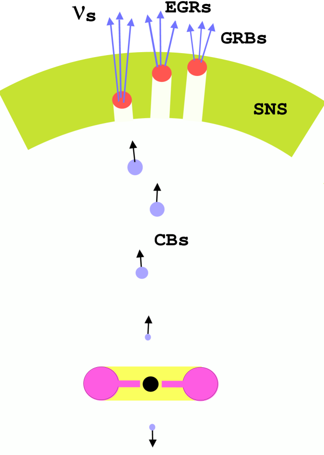
Figure 3: The CB model in a SN environment, not shown to scale. Relativistic CBs are emitted by a compact object accreting matter from a disk and/or torus. They hit a SN shell generating $\nu$’s, quasi-thermal radiation (the GRB) and $\gamma$-rays from $\pi^{0}$ decay (the EGRs). The latter two exit only from the transparent outer layers of the SN shell.

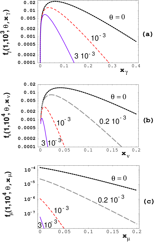
Figure 5: EGR, neutrino and muon fluxes, at various fixed observation angles $\theta$, as functions of the fractional momentum of the observed particle, at redshift unity. The functions $\rm f_{\gamma}(z,\gamma_{out},\theta,x_{\gamma})$ of Eq.(10), for $\rm\gamma_{out}=10^{3}$, and $\rm f_{\nu,\mu}(z,\gamma_{out},\theta,x_{\nu,\mu})$ of Eqs.(14, 16), both for $\rm\gamma_{in}=10^{4}$, are depicted.

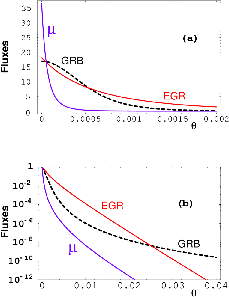
Figure 8: Comparisons of angular distributions of GRB photons, EGR photons and $\nu$-produced muons in water or ice. In the upper graph, the normalizations of the three curves are arbitrary. In the lower one, they are all normalized to unity at $\theta=0$.

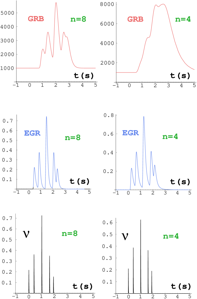
Figure 9: A “synthetic” $\gamma$-ray burst consisting of five CBs with $\rm\gamma_{out}$ within a factor of 2 of $\rm\gamma_{out}=10^{3}$, with other parameters at their reference values. The CBs are fired at random times in a 2.5 s interval. The two columns are for SNS density indices $\rm n=8$ and 4. Top: the event seen in the 30 keV to 1 MeV GRB domain. Middle: seen in EGRs from $\pi^{0}$ decay. Bottom: the neutrino signal.

References

- [1] E. Costa et al., Nature 387 (1997) 783.
- [2] J. van Paradijs et al., Nature 386 (1997) 686.
- [3] T.J. Galama et al., Nature 395 (1998) 670.
- [4] M.R. Metzger et al., Nature 387 (1997) 878.
- [5] B. Paczynski, Astroph. J. 308 (1986) L43; J. Goodman, A. Dar and S. Nussinov, Astroph. J. 314 (1987) L7.
- [6] S.E. Woosley, Astroph. J. 405 (1993) 273; S.E. Woosley and A.I. MacFadyen, Astron. and Astroph. 138 (1999) 499; A.I. MacFadyen and S.E. Woosley, Astroph. J. 524 (1999) 168.
- [7] B. Paczynski, Astroph. J. 494 (1998) L45.
- [8] N.J. Shaviv and A. Dar, Astroph. J. 447 (1995) 863.
- [9] A. Dar, Astroph. J. 500 (1998) L93.
- [10] A. Dar and A. De Rújula, astro-ph/0008474, and references therein.
- [11] A. Dar and A. De Rújula, astro-ph/0012227.
- [12] A. Dar and A. De Rújula, astro-ph/0102115.
- [13] A. Dar and A. De Rújula, astro-ph/0105094.
- [14] I.F. Mirabel and L.F. Rodriguez, Nature 371 (1994) 46, Annu. Rev. Astron. and Astroph. 37 (1999) 409, astro-ph/0007010; L.F. Rodriguez and I.F. Mirabel, Astroph. J. 511 (1999) 398.
- [15] G. Ghisellini et al., Astroph. J. 407 (1993) 65.
- [16] L. Kedziora-Chudzcu et al., Advances in Space Research 26 (2000) 727.
- [17] B. A. Margon, Annu. Rev. Astron. and Astroph. 22 (1984) 507.
- [18] T. Kotani et al., Pubs. of the Astron. Soc. of Japan 48 (1996) 619.
- [19] A. Dar, Gamma Ray Communication Network report No. GCN 346 (1999), gcncirc@lheawww.gsfc.nasa.gov.
- [20] S. Dado, A. Dar and A. De Rújula, Optical Afterglows of GRBs in the Cannonball Model, to be published.
- [21] A. Dar and R. Plaga, Astron. and Astroph. 340 (1999) 259.
- [22] A.G. Lyne and D.R. Lorimer, Nature 369 (1994) 127.
- [23] See, for instance, T. Nakamura et al., astro-ph/0007010