DESY 01-059

hep-ph/0105200

May 2001

Extended Minimal Flavour Violating MSSM and
Implications for $B$ Physics

A. Ali  and E. Lunghi

Deutsches Elektronen Synchrotron, DESY,
Notkestrasse 85, D-22607 Hamburg, Germany

The recently reported measurements of the CP asymmetry $a_{\psi K}$ by the BABAR and BELLE collaborations, obtained from the rate differences in the decays $B^{0}\to(J/\psi K_{s}),(J/\psi K_{L})$ etc., and their charge conjugates, are in good agreement with the standard model (SM) prediction of the same, resulting from the unitarity of the CKM matrix. The so-called minimal flavour violating (MFV) supersymmetric extensions of the standard model, in which the CKM matrix remains the only flavour changing structure, predict $a_{\psi K}$ similar to the one in the SM. With the anticipated precision in $a_{\psi K}$ and other CP asymmetries at the B factories and hadron colliders, one hopes to pin down any possible deviation from the SM. We discuss an extension of the MFV-supersymmetric models which comfortably accommodates the current measurements of the CP asymmetry $a_{\psi K}$, but differs from the SM and the MFV-supersymmetric models due to an additional flavour changing structure beyond the CKM matrix. We suggest specific tests in forthcoming experiments in $B$ physics. In addition to the CP-asymmetries in $B$-meson decays, such as $a_{\psi K}$ and $a_{\pi\pi}$, and the mass difference $\Delta M_{s}$ in the $B_{s}^{0}$ - $\overline{B_{s}^{0}}$ system, we emphasize measurements of the radiative transition $b\to d\gamma$ as sensitive probes of the postulated flavour changing structure. This is quantified in terms of the ratio $R(\rho\gamma/K^{*}\gamma)=2{\cal B}(B^{0}\to\rho^{0}\gamma)/{\cal B}(B^{0}\to K^{*0}\gamma)$, the isospin violating ratio $\Delta^{\pm 0}={\cal B}(B^{\pm}\to\rho^{\pm}\gamma)/2{\cal B}(B^{0}\to\rho^{0}\gamma)-1$, and the CP-asymmetry in the decay rates for $B^{+}\to\rho^{+}\gamma$ and its charge conjugate. Interestingly, the CKM–unitarity analysis in the Extended–MFV model also allows solutions $\bar{\rho}<0$ for the Wolfenstein parameter, as opposed to the SM and the MFV-supersymmetric models for which only $\bar{\rho}>0$ solutions are now admissible, implying $\gamma>\pi/2$, where $\gamma=-\arg V_{ub}$. Such large values of $\gamma$ are hinted by the current measurements of the branching ratios for the decays $B\to\pi\pi$ and $B\to K\pi$.

1 Introduction

With the advent of the B-factory era, the principal focus in flavour physics is now on measuring CP-violating asymmetries, which will determine the inner angles $\alpha$, $\beta$, and $\gamma$ of the unitarity triangle (UT) in the Cabibbo-Kobayashi-Maskawa (CKM) theory [1]. A beginning along this road has already been made through the impressive measurements of $\sin 2\beta$ by the B-factory experiments BABAR [2] and BELLE [3], following earlier leads from the OPAL [4], CDF [5, 6], and ALEPH [7] collaborations. The principal decay modes used in the measurement of $\sin 2\beta$ are $B_{d}^{0}\to J/\psi K_{S}$, $B_{d}^{0}\to\psi(2S)K_{S}$, $B_{d}^{0}\to J/\psi K_{L}$, and their charge conjugates. Concentrating on the decays $B_{d}^{0}/\overline{B_{d}^{0}}\to J/\psi K_{s}$, the time-dependent CP-asymmetry $a_{\psi K_{S}}(t)$ can be expressed as follows:

$$a_{\psi K_{S}}(t) \equiv \frac{\Gamma(B_{d}^{0}(t)\to J/\psi K_{S})-\Gamma(\overline{B_{d}^{0}}(t)\to J/\psi K_{S})}{\Gamma(B_{d}^{0}(t)\to J/\psi K_{S})+\Gamma(\overline{B_{d}^{0}}(t)\to J/\psi K_{S})}$$ (1)

$$= {\cal A}_{\rm CP}^{\rm dir}\cos(\Delta M_{B_{d}}t)+{\cal A}_{\rm CP}^{\rm mix}\sin(\Delta M_{B_{d}}t)\;,$$

where the states $B_{d}^{0}(t)$ and $\overline{B_{d}^{0}}(t)$ are understood as evolving from the corresponding initial flavour eigenstates (i.e., at $t=0$), and $\Delta M_{B_{d}}$ is the mass difference between the two mass eigenstates of the $B_{d}^{0}$ -$\overline{B_{d}^{0}}$ system, known very precisely, thanks in part due to the BABAR [8] and BELLE [9] measurements, and the present world average is $\Delta M_{B_{d}}=0.484\pm 0.010$ (ps)^-1 [10]. The quantities ${\cal A}_{\rm CP}^{\rm dir}$ and ${\cal A}_{\rm CP}^{\rm mix}$ are called the direct (i.e., emanating from the decays) and mixing-induced CP-asymmetries, respectively. Of these, the former is CKM-suppressed - a result which holds in the SM. The expectation ${\cal A}_{\rm CP}^{\rm dir}/{\cal A}_{\rm CP}^{\rm mix}\ll 1$ is supported by present data on direct CP-asymmetry in charged B-decays, $B^{\pm}\to J/\psi K^{\pm}$, yielding an upper bound on ${\cal A}_{\rm CP}^{\rm dir}$ which is already quite stringent [2, 3]. Hence, we shall assume that direct CP-asymmetry in $a_{\psi K_{S}}(t)$ is negligible and neglect the first term on the r.h.s. of Eq. (1). Recalling that ${\cal A}_{\rm CP}^{\rm mix}$ is a pure phase, one has in the SM ${\cal A}_{\rm CP}^{\rm mix}=\eta_{J/\psi K_{S}}a_{\psi K_{S}}$, with $\eta_{(J/\psi K_{S})}=-1$ being the intrinsic CP-parity of the $J/\psi K_{S}$ state, Eq. (1) simplifies to

$$a_{\psi K_{S}}(t)=-a_{\psi K_{S}}\sin(\Delta M_{B_{d}}t)~{}.$$ (2)

This relation is essentially free of hadronic uncertainties. Hence, a measurement of the left-hand-side allows to extract $a_{\psi K_{S}}$ cleanly. Note that in the SM $a_{\psi K_{S}}=\sin 2\beta$. The present world average of this quantity is [2, 3, 4, 5, 6, 7]

$$a_{\psi K_{S}}=0.79\pm 0.12~{},$$ (3)

which is dominated by the BABAR ($a_{\psi K_{S}}=0.59\pm 0.14{\rm(stat)}\pm 0.05({\rm syst}))$ [2] and BELLE ($a_{\psi K_{S}}=0.99\pm 0.14{\rm(stat)}\pm 0.06({\rm syst}))$ [3] results. We note that the current world average (which includes a scale factor following the Particle Data Group prescription [11]) based on all five experiments yields a value of $a_{\psi K_{S}}$ which is different from a null result by more than six standard deviations. To test the consistency of the SM, the current experimental value of $a_{\psi K_{S}}$ in Eq. (3) is to be compared with the indirect theoretical estimates of the same obtained from the unitarity of the CKM matrix. These latter values lie typically in the range $a_{\psi K_{S}}^{\rm SM}=0.6-0.8$ (at 68% C.L.) [12, 13, 14, 15, 16, 17, 18, 19], where the spread reflects both the uncertainties in the input parameters and treatment of errors, with most analyses yielding $a_{\psi K_{S}}^{\rm SM}\simeq 0.70$ as the central value of the CKM fits. We conclude that he current measurements of $a_{\psi K_{S}}$ are in good agreement with its indirect estimates in the SM.

The consistency of the SM with experiments on CP-violation in B-decays will come under minute scrutiny, with greatly improved accuracy on $a_{\psi K_{S}}$ and measurements of the other two angles of the UT, $\alpha$ and $\gamma$ at the $e^{+}e^{-}$ and hadronic $B$-factories. In addition, a large number of direct CP-asymmetries in charged and neutral $B$-decays, as well as flavour-changing-neutral-current (FCNC) transitions in $B$- and $K$-decays, which will be measured in the course of the next several years, will greatly help in pinning down the underlying theory of flavour physics. It is conceivable that precision experiments in flavour physics may force us to revise the SM framework by admitting new interactions, including the possibility of having new CP-violating phases. Some alternatives yielding a lower value of $a_{\psi K_{S}}$ than in the SM have already been entertained in the literature [20, 21, 22]. With the experimental situation now crystallized in Eq. (3), it now appears that the CP-asymmetry $a_{\psi K_{S}}$ has a dominantly SM origin.

In popular extensions of the SM, such as the minimal supersymmetric standard model (MSSM), one anticipates supersymmetric contributions to FCNC processes, in particular $\Delta M_{B_{d}}$, $\Delta M_{B_{s}}$ (the mass difference in the $B_{s}^{0}$ -$\overline{B_{s}^{0}}$ system), and $\epsilon_{K}$, characterizing ${\cal A}_{\rm CP}^{\rm mix}$ in the $K^{0}$ -$\overline{K^{0}}$ system. However, if the CKM matrix remains effectively the only flavour changing (FC) structure, which is the case if the quark and squark mass matrices can be simultaneously diagonalized (equivalently, the off-diagonal squark mass matrix elements are small at low energy scale), and all other FC interactions are associated with rather high scales, then all hadronic flavour transitions can be interpreted in terms of the same unitarity triangles which one encounters in the SM. In particular, in these theories $a_{\psi K_{s}}$ measures the same quantity $\sin 2\beta$ as in the SM. These models are usually called the minimal flavour violating (MFV) models, following Ref.  [23]. Despite the intrinsic dependence of the mass differences $\Delta M_{B_{d}}$, $\Delta M_{B_{s}}$, and $\epsilon_{K}$ on the underlying supersymmetric parameters, the MFV models remain very predictive and hence they have received a lot of theoretical attention lately [15, 23, 24, 25, 26, 27, 28, 29]. To summarize, in these models the SUSY contributions to $\Delta M_{B_{d}}$, $\Delta M_{B_{s}}$, and $\epsilon_{K}$ have the same CKM-dependence as the SM top quark contributions in the box diagrams (denoted below by $C_{1}^{Wtt}$). Moreover, supersymmetric effects are highly correlated and their contributions in the quantities relevant for the UT-analysis can be effectively incorporated in terms of a single common parameter $f$ by the following replacement [24, 25]:

$$\epsilon_{K},\;\Delta M_{B_{s}}\;\Delta M_{B_{d}},\;a_{\psi K_{S}}:C_{1}^{Wtt}\rightarrow C_{1}^{Wtt}(1+f)~{}.$$ (4)

The parameter $f$ is positive definite and real, implying that there are no new phases in any of the quantities specified above. The size of $f$ depends on the parameters of the supersymmetric models and the model itself [30, 31, 32, 33]. Given a value of $f$, the CKM unitarity fits can be performed in these models much the same way as they are done for the SM. Qualitatively, the CKM-fits in MFV models yield the following pattern for the three inner angles of the UT:

$$\beta^{\rm MFV}\simeq\beta^{\rm SM}~{};\;~{}~{}\gamma^{\rm MFV}<\gamma^{\rm SM}~{};\;~{}~{}\alpha^{\rm MFV}>\alpha^{\rm SM}~{}.$$ (5)

For example, a recent CKM-fit along these lines yields the following central values for the three angles [15]:

$$f = 0~{}({\rm SM}):~{}~{}(\alpha,\beta,\gamma)_{\rm central}=(95^{\circ},22^{\circ},63^{\circ})~{},$$

$$f = 0.4~{}({\rm MFV}):~{}(\alpha,\beta,\gamma)_{\rm central}=(112^{\circ},20^{\circ},48^{\circ})~{}.$$ (6)

leading to $(\sin 2\beta)^{\rm SM}_{\rm central}\simeq 0.70$ and $(\sin 2\beta)^{\rm MFV}_{\rm central}\simeq 0.64$. Thus, what concerns $\sin 2\beta$, the SM and the MFV models give similar results from the UT-fits, unless much larger values for the parameter $f$ are admitted which, as argued in Refs. [30, 31, 32, 33] and in this paper, is unlikely due to the existing constraints on the MFV-SUSY parameters.

However, in a general extension of the SM, one expects that all the quantities appearing on the l.h.s. in Eq. (4) will receive independent additional contributions. In this case, the magnitude and the phase of the off-diagonal elements in the $B_{d}^{0}$ -$\overline{B_{d}^{0}}$ and $B_{s}^{0}$ - $\overline{B_{s}^{0}}$ mass matrices can be parametrized as follows [34, 35]:

$$M_{12}(B_{d}) = {\langle\bar{B}_{d}|H_{eff}^{\Delta B=2}|B_{d}\rangle\over 2M_{B_{d}}}=r_{d}^{2}e^{2i\theta_{d}}M_{12}^{SM}(B_{d})~{},$$

$$M_{12}(B_{s}) = {\langle\bar{B}_{s}|H_{eff}^{\Delta B=2}|B_{s}\rangle\over 2M_{B_{s}}}=r_{s}^{2}e^{2i\theta_{s}}M_{12}^{SM}(B_{s})~{}.$$ (7)

where $r_{d}$ ($r_{s}$) and $\theta_{d}$ ( $\theta_{d}$) characterize, respectively, the magnitude and the phase of the new physics contribution to the mass difference $\Delta M_{B_{d}}$ ($\Delta M_{B_{s}}$). It follows that a measurement of $a_{\psi K_{s}}$ would not measure $\sin 2\beta$, but rather a combination $\sin 2(\beta+\theta_{d})$. Likewise, a measurement of the CP asymmetry in the decays $B_{d}^{0}\to\pi\pi$ and its charge conjugate, $a_{\pi\pi}$, (assuming that the penguin contributions are known) would not measure $\sin 2\alpha$, but rather $\sin 2(\alpha-\theta_{d})$. Very much along the same lines, the decay $B_{s}\to J/\psi\phi$ and its charge conjugate would yield a CP asymmetry $a_{\psi\phi}\simeq-\sin(\delta-\theta_{s})$, where $\delta\simeq 1/2\lambda^{2}\simeq 0.02$ in the SM, and $\lambda\simeq 0.22$ is one of the four CKM parameters in the Wolfenstein representation [36]. Thus, the phase $\theta_{s}$ could enhance the CP-asymmetry $a_{\psi\phi}$ bringing it within reach of the LHC-experiments [37]. In this scenario, one also expects new contributions in $M_{12}(K^{0})$, bringing in their wake additional parameters ($r_{\epsilon}$, $\theta_{\epsilon}$). They will alter the profile of CP-violation in the decays of the neutral kaons. In fact, sizable contributions from the supersymmetric sector have been entertained in the literature, though it appears now unlikely that $\epsilon_{K}$ and/or $\epsilon^{\prime}_{K}/\epsilon_{K}$ (which is a measure of direct $CP$ violation in the neutral Kaon decays) are saturated by supersymmetry [38, 39].

It is obvious that in such a general theoretical scenario, which introduces six a priori independent parameters, the predictive power vested in the CKM-UT analysis is lost. We would like to retain this predictivity, at least partially, and entertain a theoretical scenario which accommodates the current measurement in flavour physics, including the recent measurements of $a_{\psi K_{S}}$, but admits additional flavour structure. A model which incorporates these features is introduced and discussed in section 2, using the language of minimal insertion approximation (MIA) [40] in a supersymmetric context. In this framework, gluinos are assumed heavy and hence have no measurable consequences for low energy phenomenology. All FC transitions which are not generated by the CKM mixing matrix are proportional to the properly normalized off–diagonal elements of the squark mass matrices:

$$(\delta_{ij})^{U,D}_{AB}\equiv{(M^{2}_{ij})^{U,D}_{AB}\over M_{\tilde{q}_{i}}M_{\tilde{q}_{j}}}$$ (8)

where $i,j=1,2,3$ and $A,B=L,R$. We give arguments why we expect that the dominant effect of the non-CKM structure contained in the MIA-parameters is expected to influence mainly the $b\to d$ and $s\to d$ transitions while the $b\to s$ transition is governed by the MFV-SUSY and the SM contributions alone. For what concerns the quantities entering in the UT analysis, the following pattern for the supersymmetric contributions emerges in this model:

$$\Delta M_{B_{s}}: C_{1}^{Wtt}\rightarrow C_{1}^{Wtt}(1+f)$$ (9)

$$\epsilon_{K},\;\Delta M_{B_{d}},\;a_{\psi K_{S}}: C_{1}^{Wtt}\rightarrow C_{1}^{Wtt}(1+f)+C_{1}^{MI}\equiv C_{1}^{Wtt}\left(1+f+g\right)$$ (10)

where the parameters $f$ and $g=g_{R}+ig_{I}$ represent normalized (w.r.t the SM top quark $Wtt$) contributions from the MFV and MIA sectors, respectively. Thus, in the UT-analysis the contribution from the supersymmetric sector can be parametrized by two real parameters $f$ and $g_{R}$ and a parameter $g_{I}$, generating a phase $\theta_{d}$, which is in general non-zero due to the complex nature of the appropriate mass insertion parameter. We constrain these parameters, taking into account all direct and indirect bounds on the supersymmetric parameters, including the measured rates for $b\to s\gamma$ decay [41, 43, 42], $(g-2)_{\mu}$ from the Brookhaven experiment [44], and the present bound on the $b\to d\gamma$ transition, following from the experimental bound on the ratio of the branching ratios $R(\rho\gamma/K^{*}\gamma)=2{\cal B}(B^{0}\to\rho^{0}\gamma)/{\cal B}(B^{0}\to K^{*0}\gamma)$ [45]. We do not include the quantity $\epsilon_{K}^{\prime}/\epsilon_{K}$ in our analysis, despite its impeccable measurement by the NA48 [46] and KTeV [47] Collaborations, yielding the present world average ${\hbox{Re}}\,\epsilon_{K}^{\prime}/\epsilon_{K}=(1.7\pm 0.2)\times 10^{-3}$, due to the inherent non–perturbative uncertainties which have greatly reduced the impact of the $\epsilon_{K}^{\prime}/\epsilon_{K}$ measurement on the CKM phenomenology (see, for a recent review, Ref. [17]).

This model, called henceforth the Extended-MFV model, leads to a number of testable consequences, some of which are common with the more general scenarios discussed earlier in the context of Eq. (7) [34, 35]. Thus, for a certain range of the argument of the MIA parameter, this model yields $a_{\psi K_{s}}<a_{\psi K_{s}}^{\rm SM/MFV}$. For other choices of the model parameters, this model yields a higher value for this CP asymmetry. A precise measurement of $a_{\psi K_{s}}$ would fix this argument ($=\theta_{d}$) and we show its allowed range suggested by the current data. Likewise, the CP-asymmetry $a_{\pi\pi}=\sin 2(\alpha-\theta_{d})$ will be shifted from its SM-value, determined by $\theta_{d}$. All $b\to d$ transitions (leading to the decays such as $b\to d\gamma$, $b\to d\ell^{+}\ell^{-}$, $B_{d}^{0}\to\ell^{+}\ell^{-}$, where $\ell^{\pm}=e^{\pm},\mu^{\pm},\tau^{\pm}$, and the ratio of the mass differences $\Delta M_{B_{s}}/\Delta M_{B_{d}}$) may turn out to be significantly different from their SM and MFV counterparts. To illustrate this, we work out in detail the implications for the exclusive decays $B\to\rho^{0}\gamma$ and $B^{\pm}\to\rho^{\pm}\gamma$, concentrating on the (theoretically more reliable) ratios $R(\rho\gamma/K^{*}\gamma)\equiv 2{\cal B}(B^{0}\to\rho^{0}\gamma)/{\cal B}(B^{0}\to K^{*}\gamma)$, the isospin violating ratio $\Delta^{\pm 0}\equiv{\cal B}(B^{\pm}\to\rho^{\pm}\gamma)/2{\cal B}(B^{0}\to\rho^{0}\gamma)-1$, and direct CP-asymmetry in the decay rates for $B^{-}\to\rho^{-}\gamma$ and its charge conjugate. We also find that the fits of the CKM unitarity triangle in the extended MFV model, characterized by Eqs. (9) and (10) above, admit both $\bar{\rho}>0$ and $\bar{\rho}<0$ solutions, where $\bar{\rho}$ is one of the Wolfenstein parameters [36]. We illustrate this by working out the predicted values of $\gamma$ (and $\alpha$) and $\Delta M_{B_{s}}$ in this model for some specific choice of the parameters. This is in contrast with the corresponding fits in the SM and the MFV–MSSM models, which currently yield $\bar{\rho}>0$ at 2 standard deviations in the SM, with the significance increasing in the MFV–MSSM models. The allowed CKM–fits in the extended–MFV model with $\bar{\rho}<0$ imply in turn $\gamma>\pi/2$. We note that such large values of $\gamma$ are hinted by phenomenological analyses [48, 49] of the current measurements of the branching ratios for the decays $B\to K\pi,\;\pi\pi$ [50, 51, 52]. However, this inference is not yet convincing due to the present precision of data and lack of a reliable estimate of non–perturbative final state interactions in these decays.

This paper is organized as follows: In section 2, we give the outline of our extended-MFV model.The supersymmetric contributions to the quantities of interest ($\epsilon_{K}$, $\Delta M_{B_{s}}$, $\Delta M_{B_{d}}$, $a_{\psi K_{S}}$) and $R(\rho\gamma/K^{*}\gamma)$ are discussed in section 3, where we also discuss the impact of the $(g-2)_{\mu}$ experiment on our analysis. Numerical analysis of the parameters $(f,|g|)$, taking into account the experimental constraints from the $b\to s\gamma$, $b\to d\gamma$ and $(g-2)_{\mu}$, is presented in section 4. A comparative analysis of the unitarity triangle in the SM, MFV and the Extended-MFV models is described in section 5, where we also show the resulting constraints on the parameters $g_{R}$ and $g_{I}$ and the CP-asymmetry $a_{\psi K_{s}}$. The impact of the Extended-MFV model on the $b\to d\gamma$ transitions are worked out in section 6. Section 7 contains a summary and some concluding remarks. The explicit stop and chargino mass matrices are displayed in Appendix A and some loop functions encountered in the supersymmetric contributions are given in Appendix B.

2 Outline of the model

The supersymmetric model that we consider is a generalization of the model proposed in Ref. [23], based on the assumptions of Minimal Flavour Violation with heavy squarks (of the first two generations) and gluinos. The charged Higgs and the lightest chargino and stop masses are required to be heavier than $100\;{\hbox{GeV}}$ in order to satisfy the lower bounds from direct searches. The rest of the SUSY spectrum is assumed to be almost degenerate and heavier than $1\;{\hbox{TeV}}$. In this framework the lightest stop is almost right–handed and the stop mixing angle (which parameterizes the amount of the left-handed stop $\tilde{t}_{L}$ present in the lighter mass eigenstate) turns out to be of order $O(M_{W}/M_{\tilde{q}})\simeq 10\%$; for definiteness we will take $|\theta_{\tilde{t}}|\leq\pi/10$.

The assumption of a heavy ($\geq 1$ TeV) gluino totally suppresses any possible gluino–mediated SUSY contribution to low energy observables. On the other hand, the presence of only a single light squark mass eigenstate (out of twelve) has strong consequences due to the rich flavour structure which emerges from the squark mass matrices. As discussed in the preceding section, adopting the MIA-framework [40], all the FC effects which are not generated by the CKM mixing matrix are proportional to the properly normalized off–diagonal elements of the squark mass matrices (see Eq. (8)). In order to take into account the effect of a light stop, we exactly diagonalize the $2\times 2$ stop system and adopt the slightly different MIA implementation proposed in Ref. [53]. In this approach, a diagram can contribute sizably only if the inserted mass insertions involve the light stop. All other diagrams require necessarily a loop with at least two heavy ($\geq 1\;{\hbox{TeV}}$) squarks and are therefore automatically suppressed. This leaves us with only two unsuppressed flavour changing sources other than the CKM matrix, namely the mixings $\tilde{u}_{L}-\tilde{t}_{2}$ (denoted by $\delta_{\tilde{u}_{L}\tilde{t}_{2}}$) and $\tilde{c}_{L}-\tilde{t}_{2}$ (denoted by $\delta_{\tilde{c}_{L}\tilde{t}_{2}}$). We note that $\delta_{\tilde{u}_{L}\tilde{t}_{2}}$ and $\delta_{\tilde{c}_{L}\tilde{t}_{2}}$ are mass insertions extracted from the up–squarks mass matrix after the diagonalization of the stop system and are therefore linear combinations of $(\delta_{13})^{U}_{LR}$, $(\delta_{13})^{U}_{LL}$ and of $(\delta_{23})^{U}_{LR}$, $(\delta_{23})^{U}_{LL}$, respectively.

Finally, a comment on the normalization that we adopt for the mass insertions is in order. In Ref. [54] it has been pointed out that $(\delta_{i3})^{U}_{LR}$ must satisfy an upper bound of order $2m_{t}/M_{\tilde{q}_{i}}$ in order to avoid charge and colour breaking minima and directions unbounded from below in the scalar potential. We normalize the insertions relevant to our discussion so that, in the limit of light stop, they automatically satisfy this constraint:

$$\delta_{\tilde{u}(\tilde{c})_{L}\tilde{t}_{2}}\equiv{M^{2}_{\tilde{u}(\tilde{c})_{L}\tilde{t}_{2}}\over M_{\tilde{t}_{2}}M_{\tilde{q}}}{|V_{td(s)}|\over V_{td(s)}^{*}}\;.$$ (11)

This definition includes the phase of the CKM element $V_{td(s)}$. In this way, deviations from the SM predictions, for what concerns CP violating observables, will be mainly associated with complex values of the mass insertion parameters. For instance, as we will argue in the following, the CP asymmetry $a_{\psi K_{S}}$ in the decay $B\rightarrow J/\psi K_{s}$ can differ from the SM expectation only if $\arg\delta_{\tilde{u}_{L}\tilde{t}_{2}}\neq 0$. In general, the two phases must not be aligned with the respective SM-phases entering in the box diagram:

$$\arg{M^{2}_{\tilde{u}(\tilde{c})_{L}\tilde{t}_{2}}\over M_{\tilde{t}_{2}}M_{\tilde{q}}}\neq\arg V_{td(s)}^{*}\;.$$ (12)

The insertion $\delta_{\tilde{c}_{L}\tilde{t}_{2}}$ characterizes the $b\rightarrow s$ transitions and it enters in the determination of the $B_{s}-\bar{B}_{s}$ mass difference, the $b\rightarrow s\gamma$ decay rate, and observables related to other FCNC decays such as $b\to s\ell^{+}\ell^{-}$. For what concerns the $b\to s\gamma$ decay, previous analyses [55] pointed out that contributions proportional to this insertion can be as large as the SM one. The experimental results for the inclusive branching fraction are

$${\cal B}(B\rightarrow X_{s}\gamma)=\cases{(3.19\pm 0.43_{\scriptscriptstyle stat}\pm 0.27_{\scriptscriptstyle syst})\times 10^{-4}&CLEO~{}\cite[cite]{[\@@bibref{}{cleo}{}{}]}\cr(3.11\pm 0.80_{\scriptscriptstyle stat}\pm 0.72_{\scriptscriptstyle syst})\times 10^{-4}&ALEPH~{}\cite[cite]{[\@@bibref{}{aleph}{}{}]}\cr(3.36\pm 0.53_{\scriptscriptstyle stat}\pm 42_{\scriptscriptstyle syst}\pm({}^{0.50}_{0.54})_{\scriptscriptstyle model})\times 10^{-4}&BELLE~{}\cite[cite]{[\@@bibref{}{belle}{}{}]}.\cr}$$ (13)

Combining these results and adding the errors in quadrature we obtain the following world average for the inclusive branching ratio

$${\cal B}(B\rightarrow X_{s}\gamma)=(3.22\pm 0.40)\times 10^{-4}$$ (14)

yielding the following ${95\%\ \mathrm{C.L.}}$ experimentally allowed range

$$2.41\times 10^{-4}\leq{\cal B}(B\rightarrow X_{s}\gamma)\leq 4.02\times 10^{-4}\;.$$ (15)

Using the LO theoretical expression for this branching ratio, the following bound is obtained:

$$0.30\leq\left|C_{7}^{eff,LO}(m_{b})\right|\leq 0.40$$ (16)

where $C_{7}^{eff,LO}(m_{b})$ is the relevant Wilson coefficient evaluated in the LL approximation and has the value $-0.316$ in the SM. Analyses of the NLO SM [56] and SUSY [57, 23, 58, 59] contributions (for the latter only a limited class of SUSY models were considered) showed that the LO result can receive substantial corrections. Notice that the NLO analysis presented in Refs. [57, 23, 58, 59] is valid exactly for the class of models that we consider over all the SUSY parameter space (including the large $\tan\beta$ region). Implementing their formulae and allowing the SUSY input parameters to vary within the range that we will further discuss in section 4, we find that, up to few percents, the branching ratio is given by

$${\cal B}(B\rightarrow X_{s}\gamma) = 22.23\;\left[C_{7}^{eff,NLO}(m_{b})-0.061\right]^{2}+0.264\;,$$ (17)

$$C_{7}^{eff,NLO}(m_{b}) = -0.175+0.666\;C_{7}^{eff,NLO}(M_{W})+0.093\;C_{8}^{eff,NLO}(M_{W})\;.$$ (18)

The explicit expressions for $C_{7,8}^{eff,NLO}(M_{W})$ can be found in Refs. [57, 23, 58, 59]. Combining Eq. (17) and the bound (15), we obtain

$$-0.35\leq C_{7}^{eff,NLO}(m_{b})\leq-0.24\quad\quad\hbox{or}\quad\quad 0.36\leq C_{7}^{eff,NLO}(m_{b})\leq 0.49\;.$$ (19)

Notice that in Refs. [58, 59] it is pointed out that in order to get a result stable against variations of the heavy SUSY particles scale, it is necessary to properly take into account all possible SUSY contributions and to resum all the large logarithms that arise. The inclusion of the insertion $\delta_{\tilde{c}_{L}\tilde{t}_{2}}$ in this picture, in particular, should not be limited to the LO matching conditions but should instead extend to the complete NLO analysis. This program is clearly beyond the scope of the present paper. Moreover, one finds that, including the NLO corrections, the SM almost saturates the experimental branching ratio. In view of this we choose not to consider $\delta_{\tilde{c}_{L}\tilde{t}_{2}}$ in our analysis. Of course, the SUSY contribution from the MFV sector is still there, but it is real relative to the SM. The assumption of neglecting $\delta_{\tilde{c}_{L}\tilde{t}_{2}}$ will be tested in CP-asymmetries ${\cal A}_{\rm CP}(b\to s\gamma)$ and ${\cal A}_{\rm CP}(B\to K^{*}\gamma)$ at the B-factories. Notice that the exclusion of $\delta_{\tilde{c}_{L}\tilde{t}_{2}}$ from our analysis introduces strong correlations between the physics that governs $b\rightarrow d$ and $b\rightarrow s$ transitions, such as the ratio $\Delta M_{B_{s}}/\Delta M_{B_{d}}$, which would deviate from its SM (and MFV model) values.

The free parameters of the model are the common mass of the heavy squarks and gluino ($M_{\tilde{q}}$), the mass of the lightest stop ($M_{\tilde{t}_{2}}$), the stop mixing angle ($\theta_{\tilde{t}}$), the ratio of the two Higgs vevs ($\tan\beta_{S}$ ), the two parameters of the chargino mass matrix ($\mu$ and $M_{2}$), the charged Higgs mass ($M_{H^{\pm}}$) and $\delta_{\tilde{u}_{L}\tilde{t}_{2}}$. All these parameters are assumed to be real with the only exception of the mass insertion whose phase in not restricted a priori. In this way we avoid any possible problem with too large contributions to flavour conserving CP violating observables like the electric dipole moments of the leptons, hadrons and atoms.

In the next section we analyze the structure of the SUSY contributions to the observables related to the determination of the unitarity triangle, namely $\epsilon_{K}$, $\Delta M_{d,s}$ and $a_{\psi K_{S}}$.

3 SUSY contributions

The effective Hamiltonian that describes $\Delta F=2$ transitions can be written as

$${\cal{H}}_{eff}^{\Delta F=2} = -\frac{G_{F}^{2}M_{W}^{2}}{(2\pi)^{2}}(V_{tq_{1}}V_{tq_{2}}^{*})^{2}\ \left(C_{1}(\mu)\ \bar{q}^{\alpha}_{2L}\gamma^{\mu}q^{\alpha}_{1L}\cdot\bar{q}^{\beta}_{2L}\gamma_{\mu}q^{\beta}_{1L}\ +\ C_{2}(\mu)\ \bar{q}^{\alpha}_{2L}q^{\alpha}_{1R}\cdot\bar{q}^{\beta}_{2L}q^{\beta}_{1R}\right.$$ (20)

$$\left.+\ C_{3}(\mu)\ \bar{q}^{\alpha}_{2L}q^{\beta}_{1R}\cdot\bar{q}^{\beta}_{2L}q^{\alpha}_{1R}\right)+{\it h.c.}\;,$$

where $\alpha,\beta$ are colour indices and $(q_{1},q_{2})$ = $(s,d)$, $(b,d)$, $(b,s)$ for the $K$, $B_{d}$ and $B_{s}$ systems respectively.

In this framework, as previously explained, gluino contributions are negligible; therefore, we have to deal only with charged Higgs (which obeys the SM CKM structure) and chargino mediated box diagrams. Let us comment on the latter. The dominant graphs must involve exclusively the lightest stop eigenstate since the presence of an heavy ($\geq 1\;{\hbox{TeV}}$) sparticle would definitely suppress their contribution. Moreover, Feynman diagrams that contribute to $C_{3}$ are substantially suppressed with respect to diagrams that contributes to $C_{1}$. In fact, for what concerns the $B$ system, the vertices $b_{R}-\tilde{H}-\tilde{t}_{2}$ and $b_{L}-\tilde{H}-\tilde{t}_{2}$ are proportional, respectively, to $m_{b}\sin\theta_{\tilde{t}}/(\sqrt{2}M_{W}\cos\beta_{S})$ and $m_{t}\cos\theta_{\tilde{t}}/(\sqrt{2}M_{W}\sin\beta_{S})$. Their ratio is thus of order $(m_{b}/m_{t}\tan\beta_{S}\tan\theta_{\tilde{t}})^{2}$ which, even in the large $\tan\beta_{S}$ regime, is damped and not much larger than $O(0.1)$. In the K system $m_{b}$ must be replaced by $m_{s}$ and the suppression is even stronger. Notice that in frameworks in which the split between the two stop mass eigenstates is not so marked, this argument fails. Diagrams mediated by the exchange of both stops must be considered and it is possible to find regions of the parameter space (for large $\tan\beta_{S}$) in which SUSY contributions to $C_{3}$ are indeed dominant [38]. We note that, the $\tan^{4}\beta_{S}$ enhanced neutral Higgs contributions to the coefficients $C_{2,3}$, whose presence is pointed out in Ref. [60], do not impact significantly for the range of SUSY parameters that we consider ($\tan\beta_{S}<35$ and $|\theta_{\tilde{t}}|<\pi/10$).

The total contribution to $C_{1}$ can thus be written as

$$C_{1}^{tot}(M_{W})=C_{1}^{W}(M_{W})+C_{1}^{H^{\pm}}(M_{W})+C_{1}^{\chi}(M_{W})+C_{1}^{MI}(M_{W})\ .$$ (21)

The explicit expressions for the various terms are:

$$C_{1}^{W} = C_{1}^{Wtt}+\left(V_{cq_{1}}V_{cq_{2}}^{*}\over V_{tq_{1}}V_{tq_{2}}^{*}\right)^{2}C_{1}^{Wcc}+2\;{V_{cq_{1}}V_{cq_{2}}^{*}\over V_{tq_{1}}V_{tq_{2}}^{*}}\;C_{1}^{Wtc}\;,$$ (22)

$$C_{1}^{H^{\pm}} = {x_{t}^{2}\over 4\ \tan^{4}\beta_{S}}\ Y_{1}(x_{H},x_{H},x_{t},x_{t})+{x_{t}^{2}\over 2\ \tan^{2}\beta_{S}}\ Y_{1}(1,x_{H},x_{t},x_{t})$$ (23)

$$-{2x_{t}\over\tan^{2}\beta_{S}}\ Y_{2}(1,x_{H},x_{t},x_{t})\ ,$$

$$C_{1}^{\chi} = \sum_{i,j=1}^{2}\left|\tilde{V}_{i2}{m_{t}\cos\theta_{\tilde{t}}\over\sqrt{2}M_{W}\sin\beta_{S}}-\sin\theta_{\tilde{t}}\tilde{V}_{i1}^{*}\right|^{2}\left|\tilde{V}_{j2}{m_{t}\cos\theta_{\tilde{t}}\over\sqrt{2}M_{W}\sin\beta_{S}}-\sin\theta_{\tilde{t}}\tilde{V}_{j1}^{*}\right|^{2}$$ (24)

$$\times Y_{1}(x_{\tilde{t}},x_{\tilde{t}},x_{\chi_{i}},x_{\chi_{j}})\ ,$$

$$C_{1}^{MI} = \left|V_{ud}\over V_{td}\right|^{2}\sum_{i,j=1}^{2}\tilde{V}_{i1}\tilde{V}_{j1}\left(\tilde{V}_{i2}{m_{t}\cos\theta_{\tilde{t}}\over\sqrt{2}M_{W}\sin\beta_{S}}-\sin\theta_{\tilde{t}}\tilde{V}_{i1}^{*}\right)^{*}\left(\tilde{V}_{j2}{m_{t}\cos\theta_{\tilde{t}}\over\sqrt{2}M_{W}\sin\beta_{S}}-\sin\theta_{\tilde{t}}\tilde{V}_{j1}^{*}\right)^{*}$$ (25)

$$\times Y_{1}^{MI}(x_{\tilde{q}},x_{\tilde{t}},x_{\chi_{i}},x_{\chi_{j}})\;\delta_{\tilde{u}_{L}\tilde{t}_{2}}^{2}$$

$$\equiv \overline{C}_{1}^{MI}\;\delta_{\tilde{u}_{L}\tilde{t}_{2}}^{2}$$

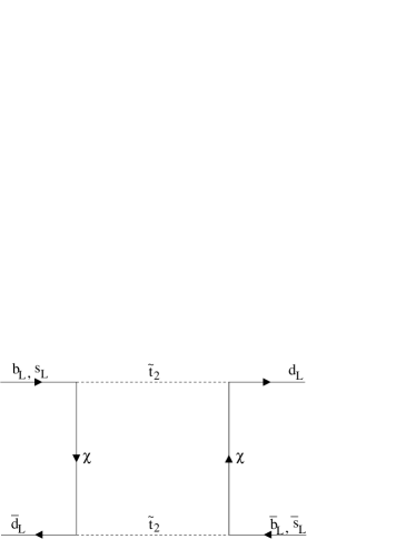
Figure 1: Feynman diagrams contributing to $C_{1}^{\chi}$ and $C_{1}^{MI}$ respectively. The bubble represents the mass insertion $\delta_{\tilde{u}_{L}\tilde{t}_{2}}$.

where $C_{1}^{W\alpha\beta}=G(x_{\alpha},x_{\beta})$ and $x_{\alpha}=m_{\alpha}^{2}/M_{W}^{2}$. The contributions to $C_{1}^{\chi}$ and $C_{1}^{MI}$ come from the Feynman diagrams shown in Fig. 1. The conventions we adopt for the chargino mass matrix, the exact definition of the stop mixing angle and the explicit expressions for the loop functions $G$, $Y_{1}$, $Y_{2}$ and $Y_{1}^{MI}$ can be found in the appendices. Notice that, if we restrict to the $B_{d}$ and $B_{s}$ cases, one may neglect the terms $C_{1}^{Wtc}$ and $C_{1}^{Wcc}$ in Eq. (22) as they are suppressed by small CKM factors. In the $K$ system, on the other hand, it is necessary to consider all the terms.

Eq. (25) describes the impact of a non–zero mass insertion on the $B_{d}$ and $K$ systems. The corresponding contribution to the $B_{s}$ system is obtained via the substitution

$$\left|V_{ud}\over V_{td}\right|^{2}\rightarrow\left|V_{us}\over V_{ts}\right|^{2}\;.$$ (26)

This implies that the impact of this diagram on the $B_{s}$ system is reduced by a factor $|V_{us}V_{td}/V_{ts}|^{2}\simeq 0.0016$ with respect to the $B_{d}$ and $K$ systems. Since, as we will show in the forthcoming analysis, $C_{1}^{MI}$ is not likely to exceed by more than twice the SM contribution, it is clear that any effect in the $B_{s}$ system from the mass insertion is completely negligible.

As already discussed in the introduction, the following structure of the SUSY contributions emerges in the class of model described above:

$$\Delta M_{B_{s}}: C_{1}^{Wtt}\rightarrow C_{1}^{Wtt}(1+f)$$

$$\epsilon_{K},\;\Delta M_{B_{d}},\;a_{\psi K_{S}}: C_{1}^{Wtt}\rightarrow C_{1}^{Wtt}(1+f)+C_{1}^{MI}\equiv C_{1}^{Wtt}\left(1+f+g\right)$$

where the parameters $f$ and $g$ represent normalized contributions from the MFV and MIA sectors, respectively,

$$f \equiv {(C_{1}^{H^{\pm}}+C_{1}^{\chi})/C_{1}^{Wtt}}$$ (27)

$$g \equiv g_{R}+ig_{I}\equiv{\overline{C}_{1}^{MI}\delta_{\tilde{u}_{L}\tilde{t}_{2}}^{2}/C_{1}^{Wtt}}\ .$$ (28)

The impact of the SUSY models on the observables we are interested in is then parametrized by three real parameters $f$, $g_{R}$ and $g_{I}$. We recall here that in the limit $g\to 0$, the above parametrization reduces to the one given in Ref. [24, 25] for the minimal flavour violation and the MSSM cases (More generally, for all models in which the CKM matrix is the only flavour–changing structure). The absence of any CKM phase in Eq. (25) as well as in the definition of $g$ reflects the definition of the mass insertion given in Eq. (11).

Note that $f$ and $g$ are functions of the SUSY parameters that enter in the computation of many other observables that are not directly related to CP violation. This implies that it is possible to look for processes that depend on the same SUSY inputs $f$ and $g$. For example, the presence of non trivial experimental bounds on the $|\Delta B=2|,~{}\Delta Q=0$ transitions can induce interesting correlations with the UT analysis. Likewise, the inclusive radiative decay $B\rightarrow X_{s}\gamma$ and $(g-2)_{\mu}$, the anomalous magnetic moment of the muon, are susceptible to supersymmetric contributions. On the other hand, it is necessary to search for observables that can put constraints on the insertion $\delta_{\tilde{u}_{L}\tilde{t}_{2}}$. In this context, the transitions $b\rightarrow d\gamma$, $B^{0}\rightarrow\rho^{0}\gamma$ and $B^{\pm}\rightarrow\rho^{\pm}\gamma$ are obvious places to look for $\delta_{\tilde{u}_{L}\tilde{t}_{2}}$–related effects.

Concerning now the $(g-2)_{\mu}$ constraint, we recall that the Brookhaven Muon $(g-2)$-collaboration has recently measured with improved precision the anomalous magnetic moment of the positive muon. The present world average for this quantity is [44]

$$a_{\mu^{+}}(\hbox{exp})=116592023(15)\times 10^{-10}\ .$$ (29)

The contribution to $a_{\mu^{+}}$ in the SM arises from the QED and electroweak corrections and from the hadronic contribution which includes both the vacuum polarization and light by light scattering [61]. The error in the SM estimate is dominated by the hadronic contribution to $a_{\mu^{+}}$ and is obtained from $\sigma(e^{+}e^{-}\rightarrow\mbox{hadrons})$ via a dispersion relation and perturbative QCD. The light-by-light hadronic contribution is, however, completely theory-driven. Several competing estimates of $a_{\mu^{+}}^{had}$ exist in the literature, reviewed recently in Ref. [62]. We briefly discuss a couple of representative estimates here.

In order to minimize the experimental errors in the low-$s$ region, Davier and Höcker supplemented the $e^{+}e^{-}\rightarrow\pi^{+}\pi^{-}$ cross section using data from tau decays. Using isospin symmetry they estimate [63]

$$a_{\mu^{+}}^{had}=(692.4\pm 6.2)\times 10^{-10}\;.$$ (30)

An updated value of $a_{\mu^{+}}^{had}$ using earlier estimates of Eidelman and Jegerlehner [64] supplemented by the recent data from CMD and BES collaborations yields [65]

$$a_{\mu^{+}}^{had}=(698.75\pm 11.11)\times 10^{-10}\;.$$ (31)

Alternatively, calculating the Adler function from $e^{+}e^{-}$ data and perturbative QCD for the tail (above $11\;{\hbox{GeV}}$) and calculating the shift in the electromagnetic fine structure constant $\Delta\alpha^{had}$ in the Euclidean region, Jegerlehner quotes [65]

$$a_{\mu^{+}}^{had}=(697.4\pm 10.45)\times 10^{-10}\;.$$ (32)

These estimates are quite compatible with each other, though the errors in Eqs. (31) and (32) are larger than in Eq. (30). Adopting the theoretical estimate from Davier and Höcker [63], one gets

$$a_{\mu^{+}}(\hbox{SM})=11659163(7)\times 10^{-10}\ ,$$ (33)

yielding

$$\delta a_{\mu^{+}}\equiv a_{\mu^{+}}(\hbox{exp})-a_{\mu^{+}}(\hbox{SM})=+43(16)\times 10^{-10},$$ (34)

which is a $2.6\;\sigma$ deviation from the SM. Using, however, the estimate from Jegerlehner in Eq. (32), gives

$$\delta a_{\mu^{+}}=+37(18)\times 10^{-10},$$ (35)

which amounts to about $2\;\sigma$ deviation from the SM. Thus, on the face-value, there exists a 2 to 2.6 $\sigma$ discrepancy between the current experiments on $(g-2)_{\mu}$ and SM-estimates.

In SUSY theories, $a_{\mu^{+}}$ receives contributions via vertex diagrams with $\chi^{0}$–$\tilde{\mu}$ and $\chi^{\pm}$–$\tilde{\nu}$ loops [61, 66, 67, 68, 69, 70, 71, 72, 73, 74, 75, 76]. The chargino diagram strongly dominates over almost all the parameter space. The chargino contribution is [66] (see also Ref. [67] for a discussion on $CP$ violating phases):

$$\delta a_{\mu^{+}}^{\chi\tilde{\nu}}={g_{2}^{2}\over 8\pi^{2}}{M_{\mu}^{2}\over M_{\tilde{\nu}}^{2}}\sum_{i=1}^{2}\left\{\left[{M_{\mu}^{2}\;{\hbox{Re}}\,(\tilde{U}_{i2}^{2})\over 2M_{W}^{2}\cos^{2}\beta_{S}}+{\hbox{Re}}\,(\tilde{V}_{i1}^{2})\right]F_{1}(x_{i})-\frac{M_{\chi_{i}}\hbox{Re}(\tilde{U}_{i2}\tilde{V}_{i1})}{\sqrt{2}M_{W}\cos\beta}F_{3}(x_{i})\right\}\;,$$ (36)

where $x_{i}=M_{\chi_{i}}^{2}/M_{\tilde{\nu}}^{2}$ and the loop functions $F_{1}$ and $F_{3}$ are given in the appendices. Eq. (36) is dominated by the last term in curly brackets whose sign is determined by $\hbox{sign}[\hbox{Re}(\tilde{U}_{12}\tilde{V}_{11})]=-\hbox{sign}[\hbox{Re}(\mu)]$ (note that we have $M_{\chi_{1}}<M_{\chi_{2}}$). Taking into account that the Brookhaven experiment implies $\delta a_{\mu^{+}}>0$ at 2 to 2.6 $\sigma$, it is clear that the $\mu>0$ region is currently favoured.

Finally let us focus on $b\rightarrow d\gamma$ decays. To the best of our knowledge, there is no direct limit on the inclusive decay $b\rightarrow d\gamma$. The present experimental upper limits on some of the exclusive branching ratios are

$${\cal B}(B^{0}\rightarrow\rho^{0}\gamma)<0.56\times 10^{-5}\;\;\;({90\%\ \mathrm{C.L.}})\mbox{\cite[cite]{[\@@bibref{}{bellebdg}{}{}]}}\;,$$ (37)

$${\cal B}(B^{+}\rightarrow\rho^{+}\gamma)<1.3\times 10^{-5}\;\;\;({90\%\ \mathrm{C.L.}})\mbox{\cite[cite]{[\@@bibref{}{cleobdg}{}{}]}}\;,$$ (38)

$$R(\rho\gamma/K^{*}\gamma)\equiv{\cal B}(B\rightarrow\rho\gamma)/{\cal B}(B\rightarrow K^{*}\gamma)<0.28\;\;\;({90\%\ \mathrm{C.L.}})\mbox{\cite[cite]{[\@@bibref{}{bellebdg}{}{}]}}\;.$$ (39)

In the numerical analysis we will use only the last constraint since the ratio of branching ratios is theoretically cleaner as only the ratio of the form factors is involved, which is calculable more reliably. Concentrating on the neutral $B$-decays, the LO expression for $R(\rho\gamma/K^{*}\gamma)$ is [78, 79]

$$R(\rho\gamma/K^{*}\gamma)={2{\cal B}(B^{0}\rightarrow\rho^{0}(770)\gamma)\over{\cal B}(B\rightarrow K^{*}\gamma)}=\left|V_{td}\over V_{ts}\right|^{2}\left(M_{B}^{2}-M_{\rho}^{2}\over M_{B}^{2}-M_{K^{*}}^{2}\right)^{3}\xi\left|C_{7}^{d}(m_{b})\over C_{7}^{s}(m_{b})\right|^{2}\;,$$ (40)

where

$$\xi=\left|F_{1}^{B^{0}\rightarrow\rho^{0}}\over F_{1}^{B^{0}\rightarrow K^{*0}}\right|^{2}\;,$$ (41)

with $F_{1}^{B^{0}\rightarrow\rho^{0},K^{*0}}$ being the form factors involving the magnetic moment (short–distance) transition; $M_{B}=5.2794\;{\hbox{GeV}}$, $M_{K^{*}}=0.8917\;{\hbox{GeV}}$, $M_{\rho^{0}}=0.7693\;{\hbox{GeV}}$ and $\xi=0.58$ [78]. $C_{7}^{(d,s)}(m_{b})$ is the Wilson coefficient of the magnetic moment operator for the transition $b\rightarrow(d,s)$ computed in the leading order approximation. Note that the annihilation contribution (which is estimated at about $25\;\%$ in $B^{\pm}\rightarrow\rho^{\pm}\gamma$ [80, 81]) is suppressed due to the unfavourable colour factor and the electric charge of the d–quark in $B^{0}$, and ignored here. In the SM, these two Wilson coefficients coincide while, in the SUSY model we consider, they differ because of the effect of the insertion $\delta_{\tilde{u}_{L}\tilde{t}_{2}}$:

$$C_{7}^{s}(M_{W}) = C_{7}^{W}(M_{W})+C_{7}^{H^{\pm}}(M_{W})+C_{7}^{\chi}(M_{W})\;,$$ (42)

$$C_{7}^{d}(M_{W}) = C_{7}^{s}(M_{W})+C_{7}^{MI}(M_{W})\;.$$ (43)

where $C_{7}^{W}$, $C_{7}^{H^{\pm}}$ and $C_{7}^{\chi}$ are, respectively, the SM, the charged Higgs and the chargino contributions and their explicit expressions can be found for instance in Refs. [57, 23]. The explicit expression for the mass insertion contribution is

$$C_{7}^{MI}(M_{W}) = \left|V_{ud}\over V_{td}\right|\sum_{i=1}^{2}{M_{\tilde{q}}M_{\tilde{t}_{2}}M_{W}\over 6M_{\chi_{i}}^{3}}\tilde{V}_{i1}\left\{\left({\tilde{V}_{i2}^{*}m_{t}\cos\theta_{\tilde{t}}\over\sqrt{2}M_{W}\sin\beta_{S}}-\tilde{V}_{i1}^{*}\sin\theta_{\tilde{t}}\right){M_{W}\over M_{\chi_{i}}}f_{1}^{MI}(x_{\tilde{t}_{2}\chi_{i}},x_{\tilde{q}\chi_{i}})\right.$$ (44)

$$\left.+{\sqrt{2}\tilde{U}_{i2}\sin\theta_{\tilde{t}}\over\cos\beta_{S}}f_{2}^{MI}(x_{\tilde{t}_{2}\chi_{i}},x_{\tilde{q}\chi_{i}})\right\}\delta_{\tilde{u}_{L}\tilde{t}_{2}}$$

$$\equiv \overline{C}_{7}^{MI}\delta_{\tilde{u}_{L}\tilde{t}_{2}}$$ (45)

where the loop functions $f_{1}^{MI}$ and $f_{2}^{MI}$ are given in Appendix B. Using Eqs. (43) and (45) it is possible to rewrite the ratio $R(\rho\gamma/K^{*}\gamma)$ in the following way:

$$R(\rho\gamma/K^{*}\gamma)=R^{SM}\left|1+\delta_{\tilde{u}_{L}\tilde{t}_{2}}{\eta^{16\over 23}\overline{C}_{7}^{MI}\over C_{7}^{s}(m_{b})}\right|^{2}$$ (46)

in which $\overline{C}_{7}^{MI}$ and $C_{7}^{s}(m_{b})$ are both real, $\eta^{16\over 23}$ is a QCD factor numerically equal to 0.66 and we have abbreviated $R(\rho\gamma/K^{*}\gamma)^{SM}$ by $R^{SM}$ for ease of writing.

4 Numerical Analysis of SUSY Contributions

In this section we study the correlations between the possible values of the parameters $f$ and $g$ as well as the numerical impact of $b\rightarrow s\gamma$, $\delta_{a_{\mu^{+}}}$ and $b\rightarrow d\gamma$ with the following experimental constraints

$$2.41\times 10^{-4}\leq{\cal B}(B\rightarrow X_{s}\gamma)\leq 4.02\times 10^{-4}\;\;\;({95\%\ \mathrm{C.L.}})$$

$$10\times 10^{-10}\leq\delta a_{\mu^{+}}\leq 74\times 10^{-10}\;\;\;({95\%\ \mathrm{C.L.}})$$ (47)

$$R(\rho\gamma/K^{*}\gamma)\leq 0.28\;\;\;({90\%\ \mathrm{C.L.}})$$

where we have used the estimates of $\delta a_{\mu^{+}}({\rm SM})$ from Eq. (30). We perform the numerical analysis by means of high density scatter plots varying the SUSY input parameters over the following ranges:

$$\cases{\makebox[39.83368pt]{$\mu$}=\;\;(100\div 1000)\;{\hbox{GeV}}\;,&\cr\makebox[39.83368pt]{$M_{2}$}=\;\;(100\div 1000)\;{\hbox{GeV}}\;,&\cr\makebox[39.83368pt]{$\tan\beta_{S}$}=\;\;3\div 35\;,&\cr\makebox[39.83368pt]{$M_{H^{\pm}}$}=\;\;(100\div 1000)\;{\hbox{GeV}}\;,&\cr\makebox[39.83368pt]{$M_{\tilde{t}_{2}}$}=\;\;(100\div 600)\;{\hbox{GeV}}\;,&\cr\makebox[39.83368pt]{$\theta_{\tilde{t}}$}=\;\;-0.3\div 0.3\;.&\cr}$$ (48)

Notice that, according to the discussion of the previous section, we restrict the scatter plot to positive $\mu$ values only. Negative values are strongly disfavoured both by the $\delta a_{\mu^{+}}\geq 0$ bound and by the $b\rightarrow s\gamma$ branching ratio. In fact, it is possible to show that if $\mu$ is negative, the chargino contributions to $b\rightarrow s\gamma$ tend to interfere constructively with the SM and the charged Higgs ones. In order not to exceed the experimental upper limit, a quite heavy SUSY spectrum is thus required. In such a situation, high $f$ and $g$ values are quite unlikely.

In Fig. 2 we plot the points in the $(f,|g|)$ plane that survive the $b\rightarrow s\gamma$, $\delta a_{\mu^{+}}$ and $b\rightarrow d\gamma$ constraints. Scanning over the parameters given in Eq. (48) we find that the constraints in Eq. (47) restrict $f$ and $|g|$ to lie essentially in the range $f<0.4$, $|g|<2.0$ . We also find that the sign of $\overline{C}_{1}^{MI}/C_{1}^{Wtt}$ is positive over all the SUSY parameter space that we scanned.

The impact of $\delta a_{\mu^{+}}$ on our analysis is not very strong, once we limit the scanning to the $\mu>0$ region only. Moreover, as follows from Eq. (36), the size of the chargino contribution to $\delta a_{\mu^{+}}$ is controlled by the mass of the muon sneutrino. In our framework, $m_{\tilde{\nu}}$ is a free parameter and we have imposed the lower bound $\delta a_{\mu^{+}}\geq 10\times 10^{-10}$ in the loosest possible way by choosing $m_{\tilde{\nu}}=100\;{\hbox{GeV}}$ (a value that is reasonably safe against direct search constraints). On the other hand, we can not reject points which give a too large contribution to $\delta a_{\mu^{+}}$ because a large enough sneutrino mass can always suppress the SUSY diagram and reduce $\delta a_{\mu^{+}}$ to a value smaller than $74\times 10^{-10}$. Notice that, if $m_{\tilde{\nu}}\geq 300\;{\hbox{GeV}}$, all the points that we consider do satisfy the upper bound: in order to obtain larger contributions it is necessary to impose a very light sneutrino mass. Only models in which the squark and the slepton mass spectra depend on the same inputs will be able to fully exploit the correlation between the anomalous magnetic moment of the muon and observables related to $B$ physics.

The impact of the $b\rightarrow d\gamma$ constraint is taken into account by imposing the following upper bound on the mass insertion:

$$\left|\delta_{\tilde{u}_{L}\tilde{t}_{2}}\right|<\left(\sqrt{0.28\over R^{SM}}-1\right)\left|C_{7}^{s}(m_{b})\over\eta^{16\over 23}\overline{C}_{7}^{MI}\right|\;.$$ (49)

Again, we find that with the current experimental bound $R(\rho\gamma/K^{*}\gamma)<0.28$, most of the otherwise allowed $(f,|g|)$ region survives. This situation will change with improved limits (or measurements of $R(\rho\gamma/K^{*}\gamma)$).

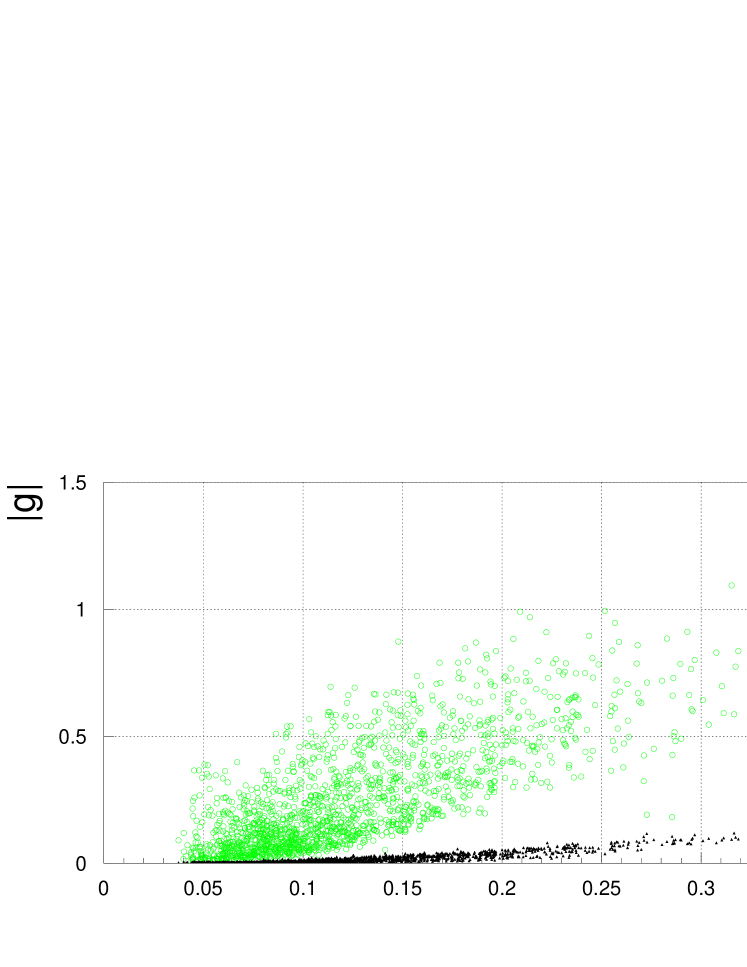
Figure 3: Allowed points in the $(f,|g|)$ plane that are compatible with a positive value of the Wilson coefficient $C_{7}$. The empty circles satisfy the $b\rightarrow s\gamma$ and $\delta a_{\mu^{+}}$ constraints. The impact of imposing in addition the upper bound on the $b\rightarrow d\gamma$ transition is represented by the black dots.

In Fig. 3 we perform the same analysis presented in Fig. 2 but we allow only for points that give a positive sign for the Wilson coefficient $C_{7}^{s}$ computed in the LO approximation. The issue whether it is possible or not to change the sign of $C_{7}^{s}$ depends on the model and has been long debated in the literature. In particular, this sign strongly characterizes the behaviour of the forward–backward asymmetry and of the dilepton invariant mass in $b\rightarrow s\ell^{+}\ell^{-}$ transitions, as well as the sign of the isospin violating ratio $\Delta$ (see below) and of the CP-violating asymmetry in the radiative decays $B\to\rho\gamma$ [79]. We use $C_{7}^{LO}$ for calculating the CP-asymmetry in $B\to\rho\gamma$. The quantity $\Delta$ in the NLO approximation requires the Wilson coefficient $C_{7}^{NLO}$. However, as shown in Ref. [79], $\Delta$ is stable against NLO vertex corrections. Recently, also the so–called hard spectator corrections have been calculated to $O(\alpha_{s})$ in $B\to\rho\gamma$ [82, 83] with the result that $\Delta$ is stable also against these corrections. We refer to Refs. [79, 84, 85, 55, 86] for a comprehensive review of the positive $C_{7}$ phenomenology. In Fig. 3, open circles represent points that satisfy the $b\rightarrow s\gamma$ and $\delta a_{\mu^{+}}$ constraints. The black dots show what happens when the experimental bound $R(\rho\gamma/K^{*}\gamma)<0.28$ is imposed. In implementing this constraint we use Eq. (49). If for a given point $\delta^{\mbox{\tiny lim}}$ turns out to be smaller than 1, we plot $|g|_{\delta=\delta^{\mbox{\tiny lim}}}$, otherwise we set $\delta=1$. It is important to note that the dependence of $C_{7}^{MI}$ and $C_{1}^{MI}$ on the mass insertion is, respectively, linear and quadratic. From Fig. 3 one sees that all the points that are compatible with a positive $C_{7}$ provide, indeed, a too large contribution to $b\rightarrow d\gamma$, and hence are effectively removed by the cut on $R(\rho\gamma/K^{*}\gamma)$. This result is quite reasonable because, in order to change the sign of $C_{7}$, a large positive chargino contribution is needed: since $C_{7}^{\chi}$ and $\overline{C}_{7}^{MI}$ depend on the same input parameters we expect their magnitude to be closely correlated. In Fig. 4, we show explicitly the correlation between $C_{7}^{s}(m_{b})$ and $\overline{C}_{7}^{MI}(m_{b})\equiv\eta^{16\over 23}\overline{C}_{7}^{MI}(M_{W})$ in both the negative and positive $C_{7}^{s}$ allowed regions. In the second plot, in particular, $|C_{7}^{MI}(m_{b})|$ turns out to be greater than one for all the points: this implies that the mass insertion constraint is always non trivial. The strong bound shown in Fig. 3 is obtained by taking into account that $g$ depends quadratically on $\delta_{\tilde{u}_{L}\tilde{t}_{2}}$. The conclusion is that if $C_{7}^{s}>0$ is experimentally established, our analysis implies strong constraints on the quantity $|g|$ from $b\to d\gamma$ decays, permitting only small deviations from the MFV-value: $|g|=0$.

5 Unitarity Triangle Analysis

In section 3 we have shown that the impact of this class of SUSY models on observables related to the unitarity triangle (UT) can be parameterized by two real parameters and by one phase (see Eqs. (9) and (10)). In this section we analyze the implications of this parametrization on the standard analysis of the UT. As usual we use the Wolfenstein parametrization [36] of the CKM matrix in terms of $\lambda$, $A$, $\rho$ and $\eta$:

$$V=\pmatrix{1-{\lambda^{2}\over 2}&\lambda&A\lambda^{3}(\rho-i\eta)\cr-\lambda&1-{\lambda^{2}\over 2}&A\lambda^{2}\cr A\lambda^{3}(1-\rho-i\eta)&-A\lambda^{2}&1\cr}\;.$$ (50)

In the following analysis we extend this parametrization beyond the leading order in $\lambda$; as a consequence it is necessary to study the unitarity triangle in the plane $(\bar{\rho},\bar{\eta})$ where $\bar{\rho}=\rho\;(1-\lambda^{2}/2)$ and $\bar{\eta}=\eta\;(1-\lambda^{2}/2)$ [87].

Let us collect the relevant formulae for $\epsilon_{K}$, $\Delta M_{B_{(d,s)}}$ and $a_{\psi K_{S}}$ as functions of $f$, $g$ and $\delta_{\tilde{c}_{L}\tilde{t}_{2}}$:

$$\epsilon_{K}=-{G_{F}^{2}f_{K}^{2}\hat{B}_{K}M_{K}M_{W}^{2}\over 12\sqrt{2}\pi^{2}\Delta M_{K}}{\hbox{Im}}\,\left\{\lambda_{c}^{*2}\eta_{cc}C_{1}^{Wcc}+2\lambda_{c}^{*}\lambda_{t}^{*}\eta_{tc}C_{1}^{Wtc}+\lambda_{t}^{*2}\eta_{tt}C_{1}^{Wtt}(1+f+g)\right\}e^{i\pi\over 4}\;,$$ (51)

$$\hskip-170.71652pt\Delta M_{B_{d}}=-{G_{F}^{2}\over 6\pi^{2}}\eta_{B}M_{B_{d}}f^{2}_{B_{d}}\hat{B}_{B_{d}}M_{W}^{2}|V_{tb}V_{td}^{*}|^{2}C_{1}^{Wtt}|1+f+g|\;,$$ (52)

$$\hskip-184.9429pt\Delta M_{B_{s}}=-{G_{F}^{2}\over 6\pi^{2}}\eta_{B}M_{B_{s}}f^{2}_{B_{s}}\hat{B}_{B_{s}}M_{W}^{2}|V_{tb}V_{ts}^{*}|^{2}C_{1}^{Wtt}(1+f)\;,$$ (53)

$$\hskip-341.43306pta_{\psi K_{S}}=\sin 2(\beta+\theta_{d})$$ (54)

where $\lambda_{q}=V_{qd}V_{qs}^{*}$, $\theta_{d}={1\over 2}\arg(1+f+g)$, $\beta$ denotes the phase of $V_{td}^{*}$ and from Eq. (50) it follows

$$\sin 2\beta={2\bar{\eta}(1-\bar{\rho})\over(1-\bar{\rho}^{2})+\bar{\eta}^{2}}\;.$$ (55)

The quantities $\eta_{tt}$, $\eta_{cc}$, $\eta_{cc}$, and $\eta_{B}$ are NLO QCD corrections. Their values together with those of the other parameters are collected in Table 1.

Parameter	Value
$\eta_{tt}$	$0.57$ [88]
$\eta_{cc}$	$1.38\pm 0.53$ [89]
$\eta_{tc}$	$0.47\pm 0.04$ [90]
$\hat{B}_{K}$	$0.94\pm 0.15$ [91, 92]
$\eta_{B}$	$0.55$ [88]
$f_{B_{d}}\sqrt{\hat{B}_{B_{d}}}$	$230\pm 40\;{\hbox{MeV}}$ [91, 92, 93]
$\xi_{s}={f_{B_{s}}\sqrt{\hat{B}_{B_{s}}}\over f_{B_{d}}\sqrt{\hat{B}_{B_{d}}}}$	$1.16\pm 0.05$ [94]

Table 1: Parameters used in the UT-fits

Our first step is to investigate the regions of the parameter space spanned by $f$, $g_{R}$ and $g_{I}$ that are allowed by the present experimental data. The procedure consists in writing the $\chi^{2}$ of the selected observables and in accepting only values of $f$ and $g$ which satisfy the condition $\min_{\rho,\eta}(\chi^{2})\leq 2$. In the computation of $\chi^{2}$ we use the following input

$$\epsilon_{K} = (2.271\pm 0.017)\;10^{-3}\mbox{[~{}PDG ~{}\cite[cite]{[\@@bibref{}{Groom}{}{}]}]},$$ (56)

$$\Delta M_{B_{d}} = 0.484\pm 0.010\;{\rm ps}^{-1}\mbox{~{}[HFWG~{}\cite[cite]{[\@@bibref{}{HFWG}{}{}]}]},$$ (57)

$$\left|V_{ub}\over V_{cb}\right| = 0.090\pm 0.025\mbox{~{}[PDG ~{}\cite[cite]{[\@@bibref{}{Groom}{}{}]}]},$$ (58)

$$a_{\psi K_{s}} = 0.79\pm 0.12\;.$$ (59)

The value quoted above for $\Delta M_{B_{d}}$ is the present world average of experiments on $B$ - $\bar{B}$ mixings, including the recent BABAR [8] and BELLE [9] measurements. We introduce the experimental data on $\Delta M_{B_{s}}$ in calculating the chi–squared ($\chi^{2}$) using the so–called amplitude method [95]. The prescription consists in adding to the $\chi^{2}$ the term $\chi^{2}_{\Delta M_{B_{s}}}=(1-\mathcal{A})^{2}/\sigma_{\mathcal{A}}^{2}$ where $\mathcal{A}$ is the amplitude of the $(B_{s}-\bar{B}_{s})$ oscillation, given by ($1\pm\mathcal{A}\cos\Delta M_{B_{s}}t$), and $\sigma_{\mathcal{A}}$ is the corresponding error. Both $\mathcal{A}$ and $\sigma_{\mathcal{A}}$ are functions of $\Delta M_{B_{s}}$. Notice that using this method, the statistical interpretation of the value of the $\chi^{2}$ in its minimum is preserved. In Ref. [96], the authors include the $\Delta M_{B_{s}}$ data using an alternative procedure. They consider a log–likelihood function referenced to $\Delta M_{B_{s}}=\infty$ and add the term $\Delta\log L^{\infty}=(1/2-\mathcal{A})/\sigma_{\mathcal{A}}$ to the $\chi^{2}$. In this way the significance of the data is increased. Notice that, in order to interpret the output of this method in terms of confidence levels it is necessary to perform a monte–carlo based analysis [97]. Since we are interested in the statistical meaning of the minimum of the $\chi^{2}$, we prefer to use the standard amplitude analysis.

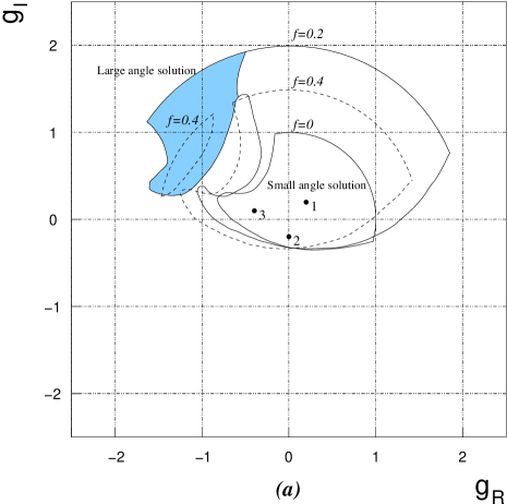
Figure 5: (a) Region of the $(g_{R},g_{I})$ plane for which $\min_{\rho,\eta}(\chi^{2})\leq 2$ from the CKM-UT fits. The $\Delta M_{B_{s}}$ constraint is taken into account using the amplitude method. The contours correspond to f = 0, 0.2 and 0.4 and the constraints on $|g|$, coming from Fig. 2, are $|g|\leq 1$, 2 and 1.5 respectively. The shaded areas correspond to a solution with $\theta+\beta>45^{\circ}$ and are allowed for $f=0.2$ and $f=0.4$. The three dots are representative points that we use to illustrate the impact of the parametrization we propose on the unitarity triangle. (b) The same as in (a), but interpreting the $2.5\;\sigma$ enhancement in the amplitude as $\Delta M_{B_{s}}=17.7\pm 1.4\;\mbox{ps}^{-1}$.

We present the output of this analysis in Fig. 5a. For each contour we fix the value of $f$ and we require the $\chi^{2}_{\rm min}$ to be less than 2. Since, as can be seen in Fig. 2, $f$ is always smaller than 0.4, we restrict the analysis to $f$ = 0, 0.2 and 0.4. Moreover, for each of these values, we require $|g|$ not to exceed the upper limit which, according to the analysis of the SUSY contributions presented in Fig. 2, we set respectively to 1, 2 and 1.5. The equation $\sin 2(\beta+\theta_{d})=a_{\psi K_{S}}$ has two solutions (mod $\pi$) in which $(\beta+\theta_{d})$ lies in the ranges $[0,\pi/4]$ and $[\pi/4,\pi/2]$ respectively. This implies that, given a value of $f$, we expect two distinct allowed regions in the $(g_{R},g_{I})$ plane, that we call respectively small and large angle solutions, characterized by $\beta+\theta_{d}<\pi/4$ (i.e. $\theta_{d}\simeq O(0.1)$ and $\beta+\theta_{d}>\pi/4$ (i.e. $\theta_{d}\simeq O(1)$). These two regions have some overlap since in the limit $a_{\psi K_{S}}=1$ (which is allowed at ${90\%\ \mathrm{C.L.}}$) the two solutions coincide. We find that, once the upper bound on $|g|$ is imposed, only a small part of the $f=0.2$ and a tiny corner of the $f=0.4$ large angle solution survive. Improvements in the experimental determination of the $B\to X_{s}\gamma$ and $B\to\rho\gamma$ branching ratios as well as more stringent lower bounds on the SUSY spectrum will have a strong impact on the allowed $|g|$ values. On the other hand, more precise measurements of $|V_{ub}/V_{cb}|$, $a_{\psi K_{S}}$, $\Delta M_{B_{s}}$ and progress in the determination of the relevant hadronic parameters, will contribute to reduce sizably the size of the allowed $(g_{R},g_{I})$ regions. In view of these considerations, we expect the large angle ($\theta_{d}\simeq O(1)$) solution is less likely to survive in future and we will concentrate in the following on the small angle scenario, i.e., $\theta_{d}\simeq O(0.1)$.

It is interesting to note that the amplitude method, that is conservatively used to set the constraint $\Delta M_{B_{s}}>14.9\;\mbox{ps}^{-1}$ at ${90\%\ \mathrm{C.L.}}$, also yields a 2.5 $\sigma$ signal for oscillations around $\Delta M_{B_{s}}=17.7\;\mbox{ps}^{-1}$. This would–be measurement is equivalent to a determination of the ratio $\Delta M_{B_{s}}/\Delta M_{B_{d}}$ which in turn depends on the precisely computed hadronic parameter $\xi_{s}$: its impact on the unitarity triangle is thus expected to be quite significant [15]. In Fig. 5b we assume this signal to be a measurement with $\Delta M_{B_{s}}=17.7\pm 1.4\;\mbox{ps}^{-1}$ in order to explore its implications on the previous analysis. The effect of the assumed value of $\Delta M_{B_{s}}$ is to reduce the $g_{R},g_{I}>0$ allowed regions; moreover, its impact is stronger the higher is the value of $f$. Note, in particular, that, with the assumed value of $\Delta M_{B_{s}}$, the $f=0.4$ contour almost disappeared. This happens because the experimentally favoured high values of $a_{\psi K_{S}}$ tend to sharpen the mismatch between the $\Delta M_{B_{d}}$ and $\Delta M_{B_{s}}/\Delta M_{B_{d}}$ constraints (which is due to a non–zero value of $f$).

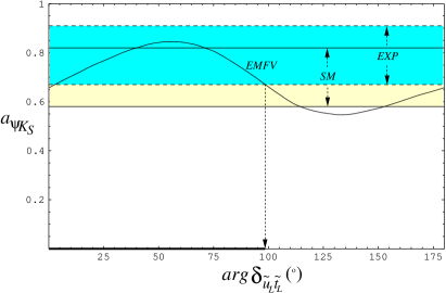
Figure 7: The $CP$ asymmetry $a_{\psi K_{S}}$ as a function of $\arg\delta_{\tilde{u}_{L}\tilde{t}_{2}}$ expressed in degrees. The solid curve corresponds to the Extended-MFV model $(f=0,\;|g|=0.28)$. The light and dark shaded bands correspond, respectively, to the allowed $1\;\sigma$ region in the SM ($0.58\leq a_{\psi K_{S}}\leq 0.82$) and the current $1\;\sigma$ experimental band ($0.67\leq a_{\psi K_{S}}\leq 0.91$). The plot on the right shows the correlation between $\arg\delta_{\tilde{u}_{L}\tilde{t}_{2}}$ and the angle $\theta_{d}$: $\theta_{d}={1\over 2}\arg(1+f+|g|e^{2i\arg\delta_{\tilde{u}_{L}\tilde{t}_{2}}}),\;(\hbox{mod}\;\pi)$. The experimentally allowed region favours $0^{\circ}<\arg\delta_{\tilde{u}_{L}\tilde{t}_{2}}<100^{\circ}$ that translates into $-3^{\circ}<\theta_{d}<8^{\circ}$.

Before concluding this section we would like to show the impact of the Extended-MFV model considered in this paper on the profile of the unitarity triangle in the $(\bar{\rho},\bar{\eta})$ plane, and the corresponding profiles in the SM and MFV models. In Fig. 6, the solid contour corresponds to the SM ${95\%\ \mathrm{C.L.}}$, the dashed one to a typical MFV case ($f=0.4$, $g=0$) and the dotted–dashed one to an allowed point in the Extended-MFV model ($f=0$, $g_{R}=-0.2$ and $g_{I}=0.2$). The representative point that we consider survives all the experimental constraints examined in the previous section. Using the values of $\bar{\rho}$ and $\bar{\eta}$ that correspond to the central value of the fit, we obtain the following results for the various observables: $|V_{ub}/V_{cb}|=0.079$, $\epsilon_{K}=2.27\times 10^{-3}$, $\Delta M_{B_{d}}=0.484\;\mbox{ps}^{-1}$, $\Delta M_{B_{s}}=20.7\;\mbox{ps}^{-1}$ and $a_{\psi K_{S}}=0.81$. If $|g|$ is sufficiently large, $\theta_{d}$ can be regarded as an essentially free parameter and the fit will choose the value that gives the best agreement with the experimental measurement. In Fig. 7 we plot the $CP$ asymmetry $a_{\psi K_{S}}$ as a function of $\arg\delta_{\tilde{u}_{L}\tilde{t}_{2}}$ (expressed in degrees). The light and dark shaded bands correspond, respectively, to the SM and the experimental $1\;\sigma$ allowed regions. The solid line is drawn for $f=0$ and $|g|=0.28$. The experimental band favours $\arg\delta_{\tilde{u}_{L}\tilde{t}_{2}}$ in the range $[0^{\circ},100^{\circ}]$. Employing the explicit dependence

$$\theta_{d}={1\over 2}\arg(1+f+|g|e^{2i\arg\delta_{\tilde{u}_{L}\tilde{t}_{2}}})\;\;\;(\hbox{mod}\;\pi)\;,$$ (60)

the above phase interval is translated into $-3^{\circ}<\theta_{d}<8^{\circ}$, for the assumed values of $|g|$ and f, which is a typical range for $\theta_{d}$ for the small angle solution with the current values of $a_{\psi K_{S}}$.

Contour	$g_{R}$	$g_{I}$	$|V_{ub}/V_{cb}|$	$\Delta M_{B_{s}}$	$a_{\psi K_{S}}$	$\alpha$	$\gamma$
1	$0.2$	$0.2$	0.094	20 $\hbox{ps}^{-1}$	0.78	$119^{\circ}$	$40^{\circ}$
2	$0.0$	$-0.2$	0.110	20 $\hbox{ps}^{-1}$	0.71	$101^{\circ}$	$51^{\circ}$
3	$-0.4$	$0.1$	0.081	17 $\hbox{ps}^{-1}$	0.73	$64^{\circ}$	$98^{\circ}$

Table 2: Central values of the CKM ratio $|V_{ub}/V_{cb}|$, the $B_{s}-\bar{B}_{s}$ mass difference $\Delta M_{B_{s}}$, the $CP$ asymmetry $a_{\psi K_{S}}$ and the inner angles $\alpha$ and $\gamma$ of the unitarity triangle for the contours in the extended–MFV model plotted in Fig. 8. The $(g_{R},g_{I})$ values for the contours are also indicated.

In order to illustrate the possible different impact of this parametrization on the unitarity triangle analysis, we focus on the $f=0$ case and choose three extremal points inside the allowed region in the plane $(g_{R},g_{I})$. We concentrate on the small angle scenario. In Fig. 8 we plot the ${95\%\ \mathrm{C.L.}}$ contours in the $(\bar{\rho},\bar{\eta})$ plane that correspond to the points we explicitely show in Fig. 5a. We summarize in Table 2 the central values of $|V_{ub}/V_{cb}|$, $\Delta M_{B_{s}}$, the $CP$ asymmetry $a_{\psi K_{S}}$, the inner angles $\alpha$ and $\gamma$ of the unitarity triangle computed for the different contours. Contour 1 is drawn for positive $g_{I}$ and $\theta_{d}$ is consequently positive. This implies that $a_{\psi K_{S}}$ is expected to be larger than in the SM. The $CP$ asymmetry and $|V_{ub}/V_{cb}|$ are very close to their world averages while the angle $\gamma$ is smaller than $\gamma^{SM}$. In contour 2 the phase $\theta_{d}$ is negative and the CP asymmetry is thus predicted to be lower than the experimental central value and still $\gamma<\gamma^{SM}$. Contour 3 is drawn for $g=-0.4+0.1i$ and is particularly interesting since it corresponds to a solution in which $a_{\psi K_{S}}$ is larger than in the SM and the Wolfenstein parameter $\bar{\rho}$ is negative, i.e. $\bar{\rho}<0$, implying a value of the inner angle $\gamma$ in the domain $\pi/2<\gamma<\pi$. This is in contrast with the SM–based analyses which currently yield $\gamma<\pi/2$ at 2 standard deviations [12, 13, 14, 15, 16, 17, 18, 19] and with the other solutions shown in Fig. 8. We note that analyses [48, 49] of the measured two–body non–leptonic decays $B\to\pi\pi$ and $B\to K\pi$ have a tendency to yield a value of $\gamma$ which lies in the range $\gamma>\pi/2$ (restricting to the solutions with $\bar{\eta}>0$). While present data, and more importantly the non–perturbative uncertainties in the underlying theoretical framework do not allow to draw quantitative conclusions at present, this may change in future. In case experimental and theoretical progress in exclusive decays force a value of $\gamma$ in the domain $\pi/2<\gamma<\pi$, the extended–MFV model discussed here would be greatly constrained and assume the role of a viable candidate to the SM.

Contour	$g_{R}$	$g_{I}$	$|V_{ub}/V_{cb}|$	$\Delta M_{B_{s}}$	$a_{\psi K_{S}}$	$\alpha$	$\gamma$
1	$0.2$	$0.2$	0.092	20 $\hbox{ps}^{-1}$	0.77	$120^{\circ}$	$40^{\circ}$
2	$0.0$	$-0.2$	0.102	20 $\hbox{ps}^{-1}$	0.65	$101^{\circ}$	$53^{\circ}$
3	$-0.4$	$0.1$	0.084	17 $\hbox{ps}^{-1}$	0.75	$64^{\circ}$	$97^{\circ}$

Table 3: The same as in Table 2. The error on $|V_{ub}/V_{cb}|$ is reduced by a factor of 2.

In Fig. 9 and Table 3 we show the consequences, on the analysis described above, of reducing the error on the CKM ratio $|V_{ub}/V_{cb}|$ by a factor of 2. The value $|V_{ub}/V_{cb}|=0.090\pm 0.013$, used by us to illustrate the improved constraint on the CKM unitarity triangle, is obtained from the inclusive measurement of $|V_{cb}|$ from CLEO [41] and LEP [98], yielding $|V_{cb}|=(40.57\pm 1.21)\times 10^{-3}$, and the average of the currently measured values of $|V_{ub}|$ by the CLEO [99] and LEP [98] groups, yielding $|V_{ub}|=(3.64\pm 0.46)\times 10^{-3}$. Note that the reduced error on $|V_{ub}/V_{cb}|$ does not affect sizably the existence of the $\bar{\rho}<0$ solution in the extended–MFV model shown here.

6 Implications of the Extended-MFV model for $b\rightarrow d\gamma$ transitions

In this section we study the implications of the extended–MFV model on the observables related to the exclusive decays $B\rightarrow\rho\gamma$, namely the ratio $R(\rho\gamma/K^{*}\gamma)$ defined in Eq. (40), the isospin breaking ratio

$$\Delta={\Delta^{+0}+\Delta^{-0}\over 2}\;,$$ (61)

where

$$\Delta^{\pm 0}={{\cal B}(B^{\pm}\rightarrow\rho^{\pm}\gamma)\over 2{\cal B}(B^{0}\rightarrow\rho^{0}\gamma)}-1\;,$$ (62)

and the $CP$ asymmetry

$$A_{CP}={{\cal B}(B^{-}\rightarrow\rho-\gamma)-{\cal B}(B^{+}\rightarrow\rho^{+}\gamma)\over{\cal B}(B^{-}\rightarrow\rho-\gamma)+{\cal B}(B^{+}\rightarrow\rho^{+}\gamma)}\;.$$ (63)

We perform the numerical analysis for following set of SUSY input parameters (that satisfy all the constraints previously discussed): $\mu=120\;{\hbox{GeV}}$, $M_{2}=350\;{\hbox{GeV}}$, $\tan\beta=4$, $M_{\tilde{t}_{2}}=280\;{\hbox{GeV}}$, $\theta_{\tilde{t}}=-0.29$ and $M_{H^{\pm}}=290\;{\hbox{GeV}}$. This allows us to exploit in detail the dependence of the various observables on the phase of the mass insertion and to give an illustrative example of the modifications in the profile of these quantities.

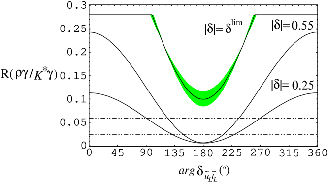
Figure 10: The ratio $R(\rho\gamma/K^{*}\gamma)={\cal B}(B\rightarrow\rho\gamma)/{\cal B}(B\rightarrow K^{*}\gamma)$ as a function of $\arg\delta_{\tilde{t}_{2}\tilde{u}_{L}}$ (in degrees) in the Extended-MFV model, satisfying the present experimental upper bound $R(\rho\gamma/K^{*}\gamma)<0.28$ (at 90% C.L.). The solid lines are obtained for $\bar{\rho}$ and $\bar{\eta}$ set to their central values and for $|\delta_{\tilde{u}_{L}\tilde{t}_{2}}|=\delta^{\mbox{\tiny lim}}$, $0.55$ and $0.25$. The shaded region in the top curve represents the $1\;\sigma$ uncertainty due to the fit of the unitarity triangle. The dashed lines indicate the $1\;\sigma$ SM prediction.

In Fig. 10 we plot the ratio $R(\rho\gamma/K^{*}\gamma)$ as a function of $\arg\delta_{\tilde{t}_{2}\tilde{u}_{L}}$ in the Extended-MFV model, and compare the resulting estimates with the SM estimates, shown by the two dashed lines representing the $1\sigma$ SM predictions. The solid curves are the SUSY results obtained for $\rho$ and $\eta$ set to their central values and for $|\delta_{\tilde{u}_{L}\tilde{t}_{2}}|=\delta^{\mbox{\tiny lim}}$, $0.55$ and $0.25$. Here, $\delta^{\mbox{\tiny lim}}$ is the absolute value of the mass insertion that saturates the experimental upper bound $R<0.28$; it is required to be smaller than 1 and it depends on the phase of the mass insertion. For the point that we consider, it varies between 0.6 (for $\arg\delta_{\tilde{t}_{2}\tilde{u}_{L}}=0,\pi$) and 1. The shaded region shown for the $|\delta_{\tilde{u}_{L}\tilde{t}_{2}}|=\delta^{\mbox{\tiny lim}}$ represents the $1\;\sigma$ uncertainty in the CKM-parameters ($\bar{\rho},\bar{\eta})$ resulting from the fit of the unitarity triangle. In the maximal insertion case, the experimental upper bound $R(\rho\gamma/K^{*}\gamma)<0.28$ is saturated for $\arg\delta_{\tilde{t}_{2}\tilde{u}_{L}}\in[0,\pi/2]\cup[3\pi/2,2\pi]$. Note that if we require the absolute value of the insertion to be maximal, the ratio $R(\rho\gamma/K^{*}\gamma)$ is always larger than in the SM. We point out that, in the extended–MFV model, this ratio does not show a strong dependence on the $\rho$ and $\eta$ values as long as these CKM parameters remain reasonably close to their allowed region. On the other hand, the impact of reducing $|\delta_{\tilde{t}_{2}\tilde{u}_{L}}|$ is quite significant.

Taking into account the discussion at the end of Sec. 3 and that $C_{7}^{s}(m_{b})$ is negative for all the points that allow for a sizable mass insertion contribution, the $\arg\delta_{\tilde{t}_{2}\tilde{u}_{L}}$ region in which the experimental bound on $R(\rho\gamma/K^{*}\gamma)$ is saturated turns out to be strongly dependent on the sign of $\overline{C}_{7}^{MI}$. Moreover, a large $\overline{C}_{7}^{MI}$ is usually associated with a large stop mixing angle whose sign determines, therefore, the overall sign of the mass insertion contribution. In our case, $\overline{C}_{7}^{MI}<0$ and the region ${\hbox{Re}}\,\delta_{\tilde{t}_{2}\tilde{u}_{L}}>0$ is consequently favoured. The qualitative behaviour of this plot can be understood rewriting Eq. (46) as

$$R(\rho\gamma/K^{*}\gamma)=R^{SM}|1+Ae^{i\arg\delta}|^{2}=R^{SM}[1+A^{2}+2A\cos(\arg\delta)]$$ (64)

where $A\equiv|\delta_{\tilde{t}_{2}\tilde{u}_{L}}|\eta^{16/23}\overline{C}_{7}^{MI}/C_{7}^{s}(m_{b})$ is positive for the point we consider.

The explicit expressions for the isospin breaking ratio and the $CP$ asymmetry in the SM are [79]

$$\Delta_{LO} = 2\epsilon_{A}\left[F_{1}+{1\over 2}\epsilon_{A}(F_{1}^{2}+F_{2}^{2})\right]\;,$$ (65)

$$A_{CP} = -{2F_{2}(A_{I}^{u}-\epsilon_{A}A_{I}^{(1)t})\over C_{7}^{SM}(m_{b})(1+\Delta_{LO})}$$ (66)

where $\epsilon_{A}=-0.3$, $A_{I}^{u}=0.046$, $A_{I}^{(1)t}=-0.016$ and

$$F_{1} = {\hbox{Re}}\,{V_{ub}V_{ud}^{*}\over V_{tb}V_{td}^{*}}\equiv-\left|V_{ub}V_{ud}^{*}\over V_{tb}V_{td}^{*}\right|\cos\alpha\;,$$ (67)

$$F_{2} = {\hbox{Im}}\,{V_{ub}V_{ud}^{*}\over V_{tb}V_{td}^{*}}\equiv-\left|V_{ub}V_{ud}^{*}\over V_{tb}V_{td}^{*}\right|\sin\alpha\;.$$ (68)

Note that $\epsilon_{A}$ is proportional to $1/C_{7}^{SM}(m_{b})$. Eqs. (65) and (66) can be easily extended to the supersymmetric case by means of the following prescriptions:

$$V_{td}^{*}\rightarrow V_{td}^{*}\;\exp\left\{i\;\arg C_{7}^{d}(m_{b})\right\}\;\;\;\;[\mbox{i.e.:}\;\alpha\rightarrow\alpha-\arg C_{7}^{d}(m_{b})]\;,$$ (69)

$$C_{7}^{SM}(m_{b})\rightarrow|C_{7}^{d}(m_{b})|\;.$$ (70)

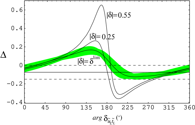
Figure 11: The isospin breaking ratio $\Delta$ as a function of $\arg\delta_{\tilde{t}_{2}\tilde{u}_{L}}$ (in degrees). See the caption in Fig. 10 for further explanations.

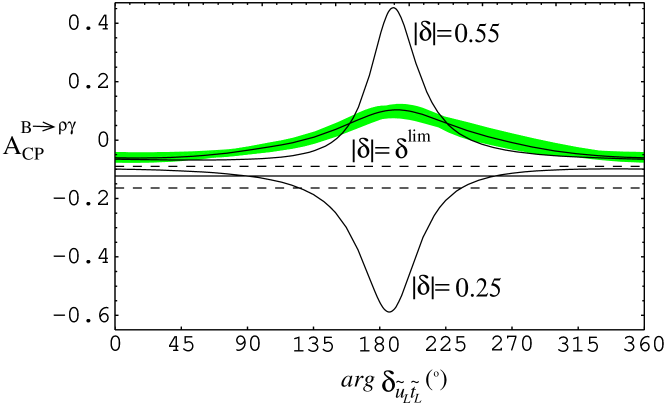
Figure 12: The $CP$ asymmetry in $B^{\pm}\rightarrow\rho^{\pm}\gamma$ as a function of $\arg(\delta_{\tilde{t}_{2}\tilde{u}_{L}})$ (in degrees). See the caption in Fig. 10 for further explanations.

In Figs. 11 and 12 we present the results of the analysis for the isospin breaking ratio and of the $CP$ asymmetry in $B^{\pm}\rightarrow\rho^{\pm}\gamma$, respectively, for the three representative cases: $|\delta_{\tilde{u}_{L}\tilde{t}_{2}}|=\delta^{\mbox{\tiny lim}}$, $0.55$ and $0.25$ in the Extended-MFV model and compare them with their corresponding SM-estimates. Since, in all likelihood, the measurement of the ratio $R(\rho\gamma/K^{*}\gamma)$ will precede the measurement of either $\Delta$ or the CP-asymmetry in $B\to\rho\gamma$ decays, the experimental value of this ratio and the CP-asymmetry $a_{\psi K_{S}}$ can be used to put bounds on $|\delta|$ and $\arg\delta_{\tilde{u}_{L}\tilde{t}_{2}}$. The measurements of $\Delta$ and the CP-asymmetry in $B^{\pm}\rightarrow\rho^{\pm}\gamma$ will then provide consistency check of this model. Concerning the cases $|\delta_{\tilde{u}_{L}\tilde{t}_{2}}|=0.55$ and $0.25$, we must underline that large deviations occur in the phase range in which an unobservably small $R(\rho\gamma/K^{*}\gamma)$ is predicted. On the other hand, it is interesting to note that, for the case of maximal insertion and for a phase compatible with the measurements of $a_{\psi K_{S}}$ (see Fig. 7), sizable deviations from the SM can occur for the $CP$ asymmetry but not for the isospin breaking ratio.

7 Summary and Conclusions

The measured $CP$ asymmetry $a_{\psi K_{S}}$ in $B$ decays is in good agreement with the SM prediction. It is therefore very likely that this $CP$ asymmetry is dominated by SM effects. Yet, the last word on this consistency will be spoken only after more precise measurements of $a_{\psi K_{S}}$ and other $CP$–violating quantities are at hand. It is possible that a consistent description of $CP$ asymmetries in $B$–decays may eventually require an additional CP-violating phase. With that in mind, we have investigated an extension of the so–called Minimal Flavour Violating version of the MSSM, and its possible implications on some aspects of $B$ physics. The non–CKM structure in this Extended-MFV model reflects the two non–diagonal mass insertions from the squark sector which influence the FCNC transitions $b\to d$ and $b\to s$ (see Eq. (11)). In the analysis presented here, we have assumed that the main effect of the mass insertions in the $B$-meson sector is contained in the $b\to d$ transition. This is plausible based on the CKM pattern of the $b\to d$ and $b\to s$ transitions in the SM. The former, being suppressed in the SM, is more vulnerable to beyond-the-SM effects. This assumption is also supported by the observation that the SM contribution in $b\to s\gamma$ decays almost saturates the present experimental measurements. We remark that the assumption of neglecting the mass insertion ($\delta_{\tilde{c}_{L}\tilde{t}_{2}}$) can be tested in the CP-asymmetry in the $b\to s$ sector, such as ${\cal A}_{\rm CP}(B\to X_{s}\gamma)$, ${\cal A}_{\rm CP}(B\to K^{*}\gamma)$, the $B_{s}^{0}$ - $\overline{B_{s}^{0}}$ mass difference $\Delta M_{B_{s}}$, and more importantly through the induced CP-asymmetry in the decay $B_{s}^{0}(\overline{B_{s}^{0}})\to J/\psi\phi$, which could become measurable in LHC experiments [37] due to the complex phase of ($\delta_{\tilde{c}_{L}\tilde{t}_{2}}$). The parameters of the model discussed here are thus the common mass of the heavy squarks and gluino ($M_{\tilde{q}}$), the mass of the lightest stop ($M_{\tilde{t}_{2}}$), the stop mixing angle ($\theta_{\tilde{t}}$), the ratio of the two Higgs vevs ($\tan\beta_{S}$), the two parameters of the chargino mass matrix ($\mu$ and $M_{2}$), the charged Higgs mass ($M_{H^{\pm}}$) and the complex insertion ($\delta_{\tilde{u}_{L}\tilde{t}_{2}}$).

We have shown that, as far as the analysis of the unitarity triangle is concerned, it is possible to encode all these SUSY effects in the present model in terms of two real parameters ($f$ and $g_{R}$) and an additional phase emerging from the imaginary part of $g$ ($g_{I}$). We find that despite the inflation of supersymmetric parameters from one ($f$ in the MFV models) to three (in the Extended-MFV models), the underlying parameter space can be effectively constrained and the model remains predictive. We have worked out the allowed region in the plane $(f,|g|=|g_{R}+ig_{I}|)$ by means of a high statistic scatter plot scanning the underlying supersymmetric parameter space, where the allowed parametric values are given in Eq. (48). The experimental constraints on the parameters emerging from the branching ratios of the decays $B\rightarrow X_{s}\gamma$ and $B\rightarrow\rho\gamma$ (implemented via the ratio $R(\rho\gamma/K^{*}\gamma)$), as well as from the recent improved determination of the magnetic moment of the muon $(g-2)_{\mu}$ were taken into account, whereby the last constraint is used only in determining the sign of the $\mu$-term.

We have done a comparative study of the SM, the MFV-models and the Extended-MFV model by performing a $\chi^{2}$-analysis of the unitarity triangle in which we have included the current world average of the $CP$ asymmetry $a_{\psi K_{S}}$ (Eq. (3)) and the current lower bound $\Delta M_{B_{s}}>14.9~{}{\rm ps}^{-1}$ using the amplitude method. Requiring the minimum of the $\chi^{2}$ to be less than two, we were able to define allowed-regions in the $(g_{R},g_{I})$ plane (correlated with the value of $f$), which are significantly more restrictive than the otherwise allowed ranges for $|g|$. We studied the dependence of the CP-asymmetry $a_{\psi K_{S}}$ on the phase of the mass insertion ($\delta_{\tilde{u}_{L}\tilde{t}_{2}}$) and find that, depending on this phase, it is possible to get both SM/MFV-like solutions for $a_{\psi K_{S}}$, as well as higher values for the CP-asymmetry. We constrain this phase to lie in the range $0^{\circ}\leq\arg\delta_{\tilde{u}_{L}\tilde{t}_{2}}\leq 100^{\circ}$, which typically yields the Extended–MFV phase $\theta_{d}$ to lie in the range $-3^{\circ}\leq\theta_{d}\leq 8^{\circ}$. The assumed measurement of the mass difference $\Delta M_{B_{s}}$, when inserted in the $\chi^{2}$ analysis, further restricts the allowed regions in $|g|$. However, as $\Delta M_{B_{s}}$ has not yet been measured, this part of the analysis is mostly illustrative. Finally, we have shown the profile of the resulting CKM–Unitarity triangle for some representative values in the extended–MFV model. They admit solutions for which $a_{\psi K_{S}}>a_{\psi K_{S}}^{\rm SM}$ and $\gamma>\gamma^{\rm SM}$, favoured by present data.

To test our model, we have focused on three observables sensitive to the mass insertion ($\delta_{\tilde{u}_{L}\tilde{t}_{2}}$) related to the radiative decays $B\rightarrow\rho\gamma$. We have worked out the consequences of the present model for the quantities $R(\rho\gamma)/R(K^{*}\gamma)=2{\cal B}(B^{0}\to\rho^{0}\gamma)/{\cal B}(B^{0}\to K^{*0}\gamma)$, the isospin violating ratio $\Delta^{\pm 0}={\cal B}(B^{\pm}\to\rho^{\pm}\gamma)/2{\cal B}(B^{0}\to\rho^{0}\gamma)-1$, and direct CP-asymmetry in the decay rates for $B\to\rho\gamma$ and its charge conjugate. We conclude that the partial branching ratios in $B\to\rho\gamma$, and hence also the ratio $R(\rho\gamma/K^{*}\gamma)$ can be substantially enhanced in this model compared to their SM-based values. The CP-asymmetry can likewise be enhanced compared to the SM value, and more importantly, it has an opposite sign for most part of the parameter space. On the other hand, it is quite difficult to obtain a significant isospin breaking ratio without suppressing the branching ratios themselves.

Finally, we remark that our analysis has led us to an interesting observation: the requirement of a positive magnetic moment Wilson coefficient (i.e., $C_{7}^{s}>0$), entering in $b\to s\gamma$ and $b\to s\ell^{+}\ell^{-}$ decays, is found to be incompatible with a sizable contribution to the parameter $g$, which encodes, in the present model, the non–CKM flavour changing contribution. Thus, it is possible to distinguish two different scenarios depending on the sign of $C_{7}^{s}$. In the $C_{7}^{s}<0$ case, as in the SM, only small deviations in the $b\to s$ phenomenology are expected, but sizable contributions to $g_{R}$ and $g_{I}$ are admissible, thereby leading to striking effects in the $b\to d$ sector. On the other hand, a positive $C_{7}^{s}$ will have strong effects in the $b\to s$ sector but, since $|g|$ will be highly constrained, the model being studied becomes a limiting case of the MFV models. In particular, in this scenario, no appreciable change in the CP-asymmetry $a_{\psi K_{s}}$ compared to the SM/MFV cases is anticipated. Since the experimental value of $a_{\psi K_{S}}$ [Eq. (3)] is in agreement with the SM/MFV–models, configurations in which $a_{\psi K_{S}}$ receives small corrections have a slight preference over the others. These aspects will be decisively tested in $B$-factory experiments.

Appendix A Stop and chargino mass matrices

The $2\times 2$ stop mass matrix is given by

$$M^{2}_{\tilde{t}}=\pmatrix{M^{2}_{\tilde{t}_{LL}}&M^{2}_{\tilde{t}_{LR}}\cr M^{2}_{\tilde{t}_{LR}}&M^{2}_{\tilde{t}_{RR}}\cr}$$ (71)

where

$$M^{2}_{\tilde{t}_{LL}} = M^{2}_{\tilde{q}}+({1\over 2}-{2\over 3}\sin^{2}\theta_{W})\cos 2\beta_{S}\,M_{Z}^{2}+M_{t}^{2}\enspace,$$ (72)

$$M^{2}_{\tilde{t}_{RR}} = M^{2}_{\tilde{q}}+{2\over 3}\sin^{2}\theta_{W}\cos 2\beta_{S}\,M_{Z}^{2}+M_{t}^{2}\enspace,$$ (73)

$$M^{2}_{\tilde{t}_{LR}} = M_{t}|A_{t}-\mu^{*}\cot(\beta_{S})|\enspace.$$ (74)

The eigenvalues are given by

$$2M^{2}_{\tilde{t}_{1},\tilde{t}_{2}}=(M^{2}_{\tilde{t}_{LL}}+M^{2}_{\tilde{t}_{RR}})\pm\sqrt{(M^{2}_{\tilde{t}_{LL}}-M^{2}_{\tilde{t}_{RR}})^{2}+4(M^{2}_{\tilde{t}_{LR}})^{2}}\enspace,$$ (75)

with $M^{2}_{\tilde{t}_{2}}\leq M^{2}_{\tilde{t}_{1}}$. We parametrize the mixing matrix ${\mathcal{R}}^{\tilde{t}}$ so that

$$\pmatrix{\tilde{t}_{1}\cr\tilde{t}_{2}}={\mathcal{R}}^{\tilde{t}}\left(\begin{array}[]{c}\tilde{t}_{L}\\ \tilde{t}_{R}\end{array}\right)=\left(\begin{array}[]{cc}\cos\theta_{\tilde{t}}&\sin\theta_{\tilde{t}}\\ -\sin\theta_{\tilde{t}}&\cos\theta_{\tilde{t}}\end{array}\right)\left(\begin{array}[]{c}\tilde{t}_{L}\\ \tilde{t}_{R}\end{array}\right)\enspace.$$ (76)

The chargino mass matrix

$$M^{\tilde{\chi}^{+}}_{\alpha\beta}=\left(\begin{array}[]{cc}M_{2}&M_{W}\sqrt{2}\sin\beta_{S}\\ M_{W}\sqrt{2}\cos\beta_{S}&\mu\end{array}\right)$$ (77)

can be diagonalized by the bi-unitary transformation

$$\tilde{U}^{*}_{j\alpha}M^{\tilde{\chi}^{+}}_{\alpha\beta}\tilde{V}^{*}_{k\beta}=M_{\tilde{\chi}_{j}^{+}}\delta_{jk}\enspace,$$ (78)

where $\tilde{U}$ and $\tilde{V}$ are unitary matrices such that $M_{\tilde{\chi}_{j}^{+}}$ are positive and $M_{\tilde{\chi}_{1}^{+}}<M_{\tilde{\chi}_{2}^{+}}$.

Appendix B Loop functions

The loop functions for box diagrams, entering in $\varepsilon_{K}$, $\Delta M_{B_{d}}$ and $\Delta M_{B_{s}}$, are,

$$G(a,b) = -\frac{ab}{4}\left({a^{2}-8a+4\over(a-b)(a-1)^{2}}\ln{a}\ +\ {b^{2}-8b+4\over(b-a)(b-1)^{2}}\ln{b}\ -\ {3\over(a-1)(b-1)}\right)\;,$$

$$Y_{1}(a,b,c,d) = {a^{2}\over(b-a)(c-a)(d-a)}\ln{a}\ +\ {b^{2}\over(a-b)(d-b)(d-b)}\ln{b}$$

$$+{c^{2}\over(a-c)(b-c)(d-c)}\ln{c}\ +\ {d^{2}\over(a-d)(b-d)(c-d)}\ln{d}\;,$$

$$Y_{2}(a,b,c,d) = \sqrt{4cd}\Bigg{[}{a\over(b-a)(c-a)(d-a)}\ln{a}\ +\ {b\over(a-b)(c-b)(d-b)}\ln{b}$$

$$+{c\over(a-c)(b-c)(d-c)}\ln{c}\ +\ {d\over(a-d)(b-d)(c-d)}\ln{d}\Bigg{]}\;,$$

$$Y_{1}^{MI}(a,b,c,d) = {Y_{1}(a,a,c,d)+Y_{1}(b,b,c,d)-2Y_{1}(a,b,c,d)\over(a-b)^{2}}\;.$$

The loop functions for penguin diagrams, entering in $b\to(s,d)\gamma$ and in the anomalous magnetic moment of the muon, are

$$F_{1}(x) = {x^{3}-6x^{2}+3x+2+6x\ln x\over 12(x-1)^{4}}\;,$$

$$F_{3}(x) = {x^{2}-4x+3+2\ln x\over 2(x-1)^{3}}\;,$$

$$f_{1}(x) = {-7+12x+3x^{2}-8x^{3}+6x(-2+3x)\log x\over 6(x-1)^{4}}\;,$$

$$f_{2}(x) = {5-12x+7x^{2}-2x(-2+3x)\log x\over 2(x-1)^{3}}\;,$$

$$f_{1,2}^{MI}(x,y) = {f_{1,2}(x)-f_{1,2}(y)\over(x-y)}\;.$$

Figure 2: Allowed points in the $(f,|g|)$ plane. The ranges of the supersymmetric parameters and the constraints from $b\rightarrow s\gamma$, $\delta a_{\mu^{+}}$ and $b\rightarrow d\gamma$ that we impose are given in Eq. (48) and Eq. (47) respectively.

Figure 4: Correlation between the SUSY contributions to $C_{7}^{s}(m_{b})$ and $\overline{C}_{7}^{MI}(m_{b})$. The plots correspond to the negative (left figure) and positive (right figure) solutions for $C_{7}^{s}(m_{b})$ allowed by the experimental bounds on ${\cal B}(B\rightarrow X_{s}\gamma)$. Note that $C_{7}^{d}(m_{b})=C_{7}^{s}(m_{b})+\overline{C}_{7}^{MI}(m_{b})\;\delta_{\tilde{u}_{L}\tilde{t}_{2}}$.

Figure 6: Allowed $95\;\%\;C.L.$ contours in the $(\bar{\rho},\bar{\eta})$ plane. The solid contour corresponds to the SM case, the dashed contour to the Minimal Flavour Violation case with $(f=0.4,\;g=0)$ and the dashed–dotted contour to the Extended-MFV model discussed in the text $(f=0,\;g_{R}=-0.2,\;g_{I}=0.2)$.

Figure 8: Allowed ${95\%\ \mathrm{C.L.}}$ contours in the $(\bar{\rho},\bar{\eta})$ plane. The solid contour is the SM case. The two semicircles represent the $2\;\sigma$ region allowed by $|V_{ub}/V_{cb}|=0.090\pm 0.025$. The contours numbered 1 to 3 correspond respectively to the points indicated in Fig. 5a, and their $(g_{R},g_{I})$ values are given in Table 2. Note that the UT–contour 3 yields $\gamma>\pi/2$.

Figure 9: The same as in Fig. 8. The error on $|V_{ub}/V_{cb}|$ is reduced by a factor of 2. The two semicircles represent the $2\;\sigma$ region allowed by $|V_{ub}/V_{cb}|=0.090\pm 0.0125$. The $(g_{R},g_{I})$ values corresponding to the three extended–MFV contours are given in Table 3.

References

-
[1]
N. Cabibbo,
Phys. Rev. Lett. 10, 531 (1963),
M. Kobayashi and T. Maskawa, Prog. Theor. Phys. 49, 652 (1973). - [2] B. Aubert et al. [BABAR Collaboration], hep-ex/0107013.
- [3] K. Abe et al. [BELLE Collaboration], hep-ex/0107061.
- [4] K. Ackerstaff et al. [OPAL Collaboration], Eur. Phys. J. C5, 379 (1998), [hep-ex/9801022].
- [5] T. Affolder et al. [CDF Collaboration], Phys. Rev. D61, 072005 (2000), [hep-ex/9909003].
- [6] C. A. Blocker [CDF Collaboration], To be published in the proceedings of 3rd Workshop on Physics and Detectors for DAPHNE (DAPHNE 99), Frascati, Italy, 16-19 Nov 1999.
- [7] R. Barate et al. [ALEPH Collaboration], Phys. Lett. B492, 259 (2000), [hep-ex/0009058].
- [8] C. Bozzi [BABAR Collaboration], (2001), hep-ex/0103046.
- [9] K. Abe et al. [BELLE Collaboration], Phys. Rev. Lett. 86, 3228 (2001), [hep-ex/0011090].
-
[10]
LEP-B-OSCILLATION Working Group, (http://lepbosc.web.cern.ch/LEPBOSC/),
Results for the Winter 2001 Conferences (XXXVIth Rencontres de Moriond: Electroweak Interactions and Unified Theories, March 10-17, 2001). - [11] Particle Data Group, D. E. Groom et al., Eur. Phys. J. C15, 1 (2000).
- [12] S. Mele, Phys. Rev. D59, 113011 (1999), [hep-ph/9810333].
- [13] S. Plaszczynski and M.-H. Schune, (1999), hep-ph/9911280.
- [14] M. Bargiotti et al., Riv. Nuovo Cim. 23N3, 1 (2000), [hep-ph/0001293].
- [15] A. Ali and D. London, Eur. Phys. J. C18, 665 (2001), [hep-ph/0012155].
- [16] M. Ciuchini et al., (2000), [hep-ph/0012308].
- [17] A. J. Buras, (2001), hep-ph/0101336.
- [18] D. Atwood and A. Soni, Phys. Lett. B508, 17 (2001), [hep-ph/0103197].
- [19] A. Hocker, H. Lacker, S. Laplace, and F. L. Diberder, (2001), hep-ph/0104062.
- [20] A. L. Kagan and M. Neubert, Phys. Lett. B492, 115 (2000), [hep-ph/0007360].
- [21] J. P. Silva and L. Wolfenstein, Phys. Rev. D63, 056001 (2001), [hep-ph/0008004].
- [22] G. Eyal, Y. Nir, and G. Perez, JHEP 08, 028 (2000), [hep-ph/0008009].
- [23] M. Ciuchini, G. Degrassi, P. Gambino, and G. F. Giudice, Nucl. Phys. B534, 3 (1998), [hep-ph/9806308].
- [24] A. Ali and D. London, Eur. Phys. J. C9, 687 (1999), [hep-ph/9903535].
- [25] A. Ali and D. London, Phys. Rept. 320, 79 (1999), [hep-ph/9907243].
- [26] A. J. Buras, P. Gambino, M. Gorbahn, S. Jager, and L. Silvestrini, Phys. Lett. B500, 161 (2001), [hep-ph/0007085].
- [27] A. J. Buras and R. Buras, Phys. Lett. B501, 223 (2001), [hep-ph/0008273].
- [28] A. Bartl et al., (2001), hep-ph/0103324.
- [29] A. J. Buras and R. Fleischer, (2001), hep-ph/0104238.
- [30] T. Nihei, Prog. Theor. Phys. 98, 1157 (1997), [hep-ph/9707336].
- [31] T. Goto, Y. Okada, and Y. Shimizu, (1999), hep-ph/9908499.
- [32] T. Goto, Y. Y. Keum, T. Nihei, Y. Okada, and Y. Shimizu, Phys. Lett. B460, 333 (1999), [hep-ph/9812369].
- [33] S. Baek and P. Ko, Phys. Rev. Lett. 83, 488 (1999), [hep-ph/9812229].
- [34] A. G. Cohen, D. B. Kaplan, F. Lepeintre, and A. E. Nelson, Phys. Rev. Lett. 78, 2300 (1997), [hep-ph/9610252].
- [35] J. P. Silva and L. Wolfenstein, Phys. Rev. D55, 5331 (1997), [hep-ph/9610208].
- [36] L. Wolfenstein, Phys. Rev. Lett. 51, 1945 (1983).
- [37] P. Ball et al., (2000), hep-ph/0003238.
- [38] D. A. Demir, A. Masiero, and O. Vives, Phys. Rev. Lett. 82, 2447 (1999), [hep-ph/9812337].
- [39] S. Baek, J. H. Jang, P. Ko, and J. H. Park, Phys. Rev. D62, 117701 (2000), [hep-ph/9907572].
- [40] L. J. Hall, V. A. Kostelecky, and S. Raby, Nucl. Phys. B267, 415 (1986).
- [41] D. Cassel [CLEO Collaboration], talk presented at the XX International Symposium on Lepton and Photon Interactions at High Energies, Rome, Italy, Jul. 23-28, 2001. (To be published in the proceedings).
- [42] R. Barate et al. [ALEPH Collaboration], Phys. Lett. B429, 169 (1998).
- [43] K. Abe et al. [BELLE Collaboration], Phys. Lett. B 511 (2001) 151 [hep-ex/0103042].
- [44] H. N. Brown et al. [Muon g-2 Collaboration], Phys. Rev. Lett. 86, 2227 (2001), [hep-ex/0102017].
- [45] A. Abashian et al. [BELLE Collaboration], BELLE-CONF-0003 (2000).
- [46] H. Wahl [NA48 Collaboration], A new measurement of direct CP–violation by NA48 (DESY Seminar, 26/06/2001).
- [47] A. Glazov [KTeV Collaboration], New measurement of the direct CP–violating parameter by the KTeV Collaboration (DESY Seminar, 19/06/2001).
- [48] W.-S. Hou and K.-C. Yang, Phys. Rev. Lett. 84, 4806 (2000), [hep-ph/9911528].
- [49] M. Beneke, G. Buchalla, M. Neubert, and C. T. Sachrajda, (2001), hep-ph/0104110.
- [50] D. Cronin-Hennessy et al. [CLEO Collaboration], Phys. Rev. Lett. 85, 515 (2000).
- [51] L. Cavolo [BABAR Collaboration], Talk presented at the XXXVIth Rencontres de Moriond, Electroweak Interactions and Unified Theories, Les Arcs, France, March 2001.
- [52] T. Ijima [BELLE Collaboration], Talk presented at the International Conference on B Physics and CP Violation (BCP4), se–Shima, Japan, 19-23 February 2001 .
- [53] A. J. Buras, A. Romanino, and L. Silvestrini, Nucl. Phys. B520, 3 (1998), [hep-ph/9712398].
- [54] J. A. Casas and S. Dimopoulos, Phys. Lett. B387, 107 (1996), [hep-ph/9606237].
- [55] E. Lunghi, A. Masiero, I. Scimemi, and L. Silvestrini, Nucl. Phys. B568, 120 (2000), [hep-ph/9906286].
- [56] K. Chetyrkin, M. Misiak, and M. Münz, Phys. Lett. B400, 206 (1997), Erratum-ibid. B 425 (1997) 414, [hep-ph/9612313].
- [57] M. Ciuchini, G. Degrassi, P. Gambino, and G. F. Giudice, Nucl. Phys. B527, 21 (1998), [hep-ph/9710335].
- [58] G. Degrassi, P. Gambino, and G. F. Giudice, JHEP 12, 009 (2000), [hep-ph/0009337].
- [59] M. Carena, D. Garcia, U. Nierste, and C. E. M. Wagner, Phys. Lett. B499, 141 (2001), [hep-ph/0010003].
- [60] A. J. Buras, P. H. Chankowski, J. Rosiek and L. Slawianowska, hep-ph/0107048.
- [61] A. Czarnecki and W. J. Marciano, Nucl. Phys. Proc. Suppl. 76, 245 (1999), [hep-ph/9810512]; (2001), hep-ph/0102122.
- [62] W. J. Marciano and B. L. Roberts, (2001), hep-ph/0105056.
- [63] M. Davier and A. Hocker, Phys. Lett. B435, 427 (1998), [hep-ph/9805470].
-
[64]
S. Eidelman and F. Jegerlehner,
Z. Phys. C67, 585 (1995), [hep-ph/9502298];
S. Eidelman and F. Jegerlehner, Nucl. Phys. Proc. Suppl. 51C, 131 (1996), [hep-ph/9606484]. - [65] F. Jegerlehner, (2001), hep-ph/0104304.
- [66] T. Moroi, Phys. Rev. D53, 6565 (1996), [hep-ph/9512396].
-
[67]
T. Ibrahim and P. Nath,
Phys. Rev. D61, 095008 (2000), [hep-ph/9907555];
T. Ibrahim and P. Nath, Phys. Rev. D61, 015004 (2000), [hep-ph/9908443]. - [68] L. L. Everett, G. L. Kane, S. Rigolin, and L.-T. Wang, Phys. Rev. Lett. 86, 3484 (2001), [hep-ph/0102145].
- [69] J. L. Feng and K. T. Matchev, Phys. Rev. Lett. 86, 3480 (2001), [hep-ph/0102146].
- [70] E. A. Baltz and P. Gondolo, (2001), hep-ph/0102147.
- [71] U. Chattopadhyay and P. Nath, (2001), hep-ph/0102157.
- [72] S. Komine, T. Moroi, and M. Yamaguchi, Phys. Lett. B506, 93 (2001), [hep-ph/0102204].
- [73] J. Ellis, D. V. Nanopoulos, and K. A. Olive, (2001), hep-ph/0102331.
- [74] S. P. Martin and J. D. Wells, (2001), hep-ph/0103067.
- [75] D. F. Carvalho, J. Ellis, M. E. Gomez, and S. Lola, (2001), hep-ph/0103256.
- [76] H. Baer, C. Balazs, J. Ferrandis, and X. Tata, (2001), hep-ph/0103280.
- [77] CLEO, T. E. Coan et al., Phys. Rev. Lett. 84, 5283 (2000), [hep-ex/9912057].
- [78] A. Ali, V. M. Braun, and H. Simma, Z. Phys. C63, 437 (1994), [hep-ph/9401277].
- [79] A. Ali, L. T. Handoko, and D. London, Phys. Rev. D63, 014014 (2000), [hep-ph/0006175].
- [80] A. Khodjamirian, G. Stoll, and D. Wyler, Phys. Lett. B358, 129 (1995), [hep-ph/9506242].
- [81] A. Ali and V. M. Braun, Phys. Lett. B359, 223 (1995), [hep-ph/9506248].
- [82] A. Ali and A. Y. Parkhomenko, (2001), hep-ph/0105302.
- [83] S. W. Bosch and G. Buchalla, (2001), hep-ph/0106081.
- [84] P. Cho, M. Misiak, and D. Wyler, Phys. Rev. D54, 3329 (1996), [hep-ph/9601360].
- [85] A. Ali, P. Ball, L. T. Handoko, and G. Hiller, Phys. Rev. D61, 074024 (2000), [hep-ph/9910221].
- [86] F. Krüger and E. Lunghi, Phys. Rev. D63, 014013 (2001), [hep-ph/0008210].
- [87] A. J. Buras, M. E. Lautenbacher, and G. Ostermaier, Phys. Rev. D50, 3433 (1994), [hep-ph/9403384].
- [88] A. J. Buras, M. Jamin, and P. H. Weisz, Nucl. Phys. B347, 491 (1990).
- [89] S. Herrlich and U. Nierste, Nucl. Phys. B419, 292 (1994), [hep-ph/9310311].
- [90] S. Herrlich and U. Nierste, Phys. Rev. D52, 6505 (1995), [hep-ph/9507262].
- [91] T. Draper, Nucl. Phys. Proc. Suppl. 73, 43 (1999), [hep-lat/9810065].
- [92] S. R. Sharpe, (1998), hep-lat/9811006.
- [93] C. Bernard, Nucl. Phys. Proc. Suppl. 94, 159 (2001), [hep-lat/0011064].
- [94] C. Bernard et al., Phys. Rev. Lett. 81, 4812 (1998), [hep-ph/9806412].
- [95] H. G. Moser and A. Roussarie, Nucl. Instrum. Meth. A384, 491 (1997).
- [96] P. Checchia, E. Piotto, and F. Simonetto, (1999), hep-ph/9907300.
-
[97]
G. Boix and D. Abbaneo,
JHEP 08, 004 (1999), [hep-ex/9909033];
M. Ciuchini et al., (2000), hep-ph/0012308. - [98] Heavy Flavour Steering Group, http://lephfs.web.cern.ch/LEPHFS.
- [99] B. H. Behrens et al. [CLEO Collaboration], Phys. Rev. D 61 (2000) 052001 [hep-ex/9905056].