${\partial m\over\partial\mu}$ in the Nambu–Jona-Lasinio model

Abstract

Using the Nambu–Jona-Lasinio (NJL) model we study responses of the pion and kaon masses to changes in the chemical potential, ${\partial m\over\partial\mu}$, at zero and finite chemical potential. We find that the behavior of ${\partial m\over\partial\mu}$ for the pion is quite different from that for the kaon. Our results can give a clue for future studies of ${\partial m\over\partial\mu}$ on the lattice.

1. Introduction

There are several methods to understand the behavior of matter under extreme conditions of temperature and/or density. One of them is the lattice QCD. While the structure of QCD at high temperature has been investigated in detail, little is known about matter at high baryon density due to the well-known “complex-action” problem lattice . One of possible ways on the lattice is to simulate the response of a hadron mass to changes in the chemical potential, ${\partial m\over\partial\mu}$, at zero chemical potential ($\mu$ = 0) taro ; miyamura .

One the other hand, one can use effective models of QCD : e.g., the NJL model njl . This model has been widely used for describing the phase transition as well as hadron properties in hot and/or dense matter hk94 .

In this work we present the NJL model calculations of ${\partial m\over\partial\mu}$ for the pion and kaon. The primary goal of our study is to get the same quantities which are simulated on the lattice. Of course, the direct comparison between the lattice data and the NJL model calculations is not possible because ${\partial m\over\partial\mu}$ on the lattice is for the screening mass while for the pole mass in the NJL model. Nevertheless, we can learn some ideas for future studies of ${\partial m\over\partial\mu}$ on the lattice from this effective model calculations.

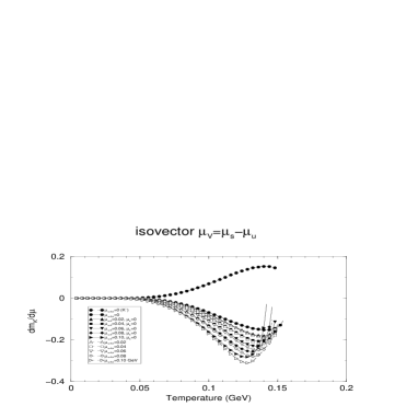
Following the notation of the lattice simulations we consider two kinds of the chemical potential. One is the isoscalar $\mu_{S}$ = $\mu_{u}$ + $\mu_{s}$ for the kaon (or $\mu_{u}$ + $\mu_{d}$ for the pion). The other is the isovector $\mu_{V}$ = $\mu_{s}$ – $\mu_{u}$ (or $\mu_{d}$ – $\mu_{u}$). In contrast to the lattice simulations we get ${\partial m\over\partial\mu}$ at zero and finite chemical potential within the NJL model. Then, our study can give information about the role of the light quark chemical potential and/or the strange quark chemical potential in hot and/or dense matter.

The paper is organized as follows. In Sec. 2 we introduce some basic formulas to get ${\partial m_{K}\over\partial\mu}$ for the kaon in the NJL model, and show results at zero and finite chemical potential. We present ${\partial m_{\pi}\over\partial\mu}$ for the pion in Sec. 3. In Sec. 4 we summarize our results and discuss some uncertainties in our calculations.

2. ${\partial m_{K}\over\partial\mu}$ in the NJL model

We use the generalized SU(3) NJL model with the anomaly term hk94 :

$${\em L}=\bar{q}(i\gamma\cdot\partial-m)q+{1\over 2}g_{S}\sum_{a=0}^{8}\left[(\bar{q}\lambda_{a}q)^{2}+\bar{q}(i\lambda_{a}\gamma_{5}q)^{2}\right]+g_{D}\left[{\rm det}~{}\bar{q}_{i}(1-\gamma_{5})q_{j}+h.c.\right]\ ,$$ (1)

where $\lambda_{a}$ are the Gell-Mann matrices and $m$ is a mass matrix for current quarks, $m$ = diag($m_{u}$, $m_{d}$, $m_{s}$). We take the following parameters in hk94 .

$$\Lambda=631.4~{}{\rm MeV},~{}g_{S}\Lambda^{2}=3.67,~{}g_{D}\Lambda^{5}=-9.29$$

$$m_{u}=m_{d}=5.5~{}{\rm MeV},~{}m_{s}=135.7~{}{\rm MeV}\ ,$$ (2)

where $\Lambda$ is the momentum cut-off. The third term in Eq.(1) is a reflection of the axial anomaly, and causes a mixing in flavors. For example, the constituent quark masses are given as follows.

$$M_{u} = m_{u}-2g_{S}\alpha-2g_{D}\beta\gamma\ ,$$

$$M_{d} = m_{d}-2g_{S}\beta-2g_{D}\alpha\gamma\ ,$$

$$M_{s} = m_{s}-2g_{S}\gamma-2g_{D}\alpha\beta\ ,$$ (3)

where $\alpha\equiv\langle\bar{u}u\rangle$, $\beta\equiv\langle\bar{d}d\rangle$, and $\gamma\equiv\langle\bar{s}s\rangle$. It means that a change of $\langle\bar{u}u\rangle$ results in a change of $\langle\bar{s}s\rangle$, and vice versa. Then, we can expect a change in the properties of the observables related with the strange quarks even in the nuclear matter.

In this work we concentrate mostly on the Case II in hk94 , where only $g_{D}$ has a $T$-dependence

$$g_{D}(T)=g_{D}(T=0)~{}{\rm exp}[-(T/T_{0})^{2}]$$ (4)

while other coupling constants and the cut-off are independent of $T$ and chemical potential (or density). Here, we set $T_{0}$ = 0.1 GeV taking into account the restoration of $U_{A}(1)$ symmetry as in hk94 . It might be realistic to make the coupling constants and/or the cut-off dependent on temperature and chemical potential. However, at present, there is no such an estimate including all variations in the cut-off and the coupling constants except for a few estimates of the strength of the anomaly term $g_{D}$ gdt .

In the mean-field approximation the above Lagrangian leads to the following gap equation hk94 .

$$\langle\bar{q}_{i}q_{i}\rangle=2N_{c}\sum_{p}\left({-M_{i}\over E_{ip}}f(E_{ip})\right)\ ,$$ (5)

where $\langle\cdot\rangle$ means the statistical average and the index $i$ denotes the $u$, $d$, and $s$ quarks. $N_{c}$ is the number of colors and $M_{i}$ is the constituent quark mass, and $E_{ip}=\sqrt{M_{i}^{2}+p^{2}}$. $f(E_{ip})=1-n_{ip}-\bar{n}_{ip}$, where $n_{ip}$ and $\bar{n}_{ip}$ are the distribution functions of the $i$th quark and antiquark, respectively.

$$n_{ip}={1\over 1+{\rm exp}~{}((E_{ip}-\mu_{i})/T)}\ ,$$

$$\bar{n}_{ip}={1\over 1+{\rm exp}~{}((E_{ip}+\mu_{i})/T)}\ .$$ (6)

The right-hand side of Eq.(5) is a function of $F~{}(\langle\bar{u}u\rangle,\langle\bar{d}d\rangle,\langle\bar{s}s\rangle,\mu_{i},T)$. Then, we obtain responses of the quark condensates ${\partial\langle\bar{u}u\rangle\over\partial\mu}$, ${\partial\langle\bar{d}d\rangle\over\partial\mu}$, and ${\partial\langle\bar{s}s\rangle\over\partial\mu}$ by differentiating both sides with respect to $\mu$ at a fixed $T$. These ${\partial\langle\bar{q}q\rangle\over\partial\mu}$ will be used to get ${\partial m_{K}\over\partial\mu}$ in the below.

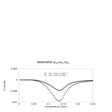
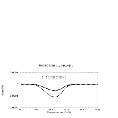
Fig.1 shows ${\partial\langle\bar{u}u\rangle\over\partial\mu_{S}}$ and ${\partial\langle\bar{s}s\rangle\over\partial\mu_{S}}$ at finite chemical potential. At zero chemical potential both ${\partial\langle\bar{q}q\rangle\over\partial\mu_{S}}$ and ${\partial\langle\bar{q}q\rangle\over\partial\mu_{V}}$ are zero. We take two different values for the chemical potential, $\mu_{u}$ = $\mu_{d}$ = 0.02 and 0.04 GeV. In the figure we set the perpendicular axis as the absolute value of ${\partial\langle\bar{q}q\rangle\over\partial\mu_{S}}$ , i.e. ${\partial|\langle\bar{q}q\rangle|\over\partial\mu_{S}}$, and thus the figure shows that the absolute value of the quark condensate decreases with increasing chemical potential. In addition, the figure shows that variations of the $u$ quark condensate ${\partial\langle\bar{u}u\rangle\over\partial\mu_{S}}$ are much larger than those of ${\partial\langle\bar{s}s\rangle\over\partial\mu_{S}}$, and the variation of each quark condensate is proportional to the chemical potential.

         

Figure 1: The responses of the $u$ (left) and $s$ (right) quark condensates.

Figure 2: ${\partial m_{K}\over\partial\mu_{S}}$ for the $K^{-}$ at zero chemical potential.

         

Figure 3: ${\partial m_{K}\over\partial\mu}$ for the $K^{-}$.

         

Figure 4: ${\partial m_{K}\over\partial\mu}$ for the $K^{+}$.

Now, consider the dispersion equation for the kaon, e.g., the $K^{-}$ hk94 .

$$D^{R}_{K^{-}}(\omega,\vec{q}=0)^{-1}\equiv-G_{K}^{-1}\left[1+2G_{K}I^{p}_{su}(\omega,\vec{q}=0)\right]=0\ ,$$ (7)

where $G_{K}$ is the coupling strength in this channel, $G_{K}\equiv g_{S}+g_{D}\beta$, and $I^{p}_{su}(\omega,\vec{q}=0)$ is the one-loop polarization due to $u$- and $s$-quarks. Differentiating both sides of the above equation with respect to $\mu_{S}$ (or $\mu_{V}$) at the fixed $T$, and using ${\partial\langle\bar{q}q\rangle\over\partial\mu_{S}}$ (or ${\partial\langle\bar{q}q\rangle\over\partial\mu_{V}}$) we get ${\partial m_{K}\over\partial\mu_{S}}$ (or ${\partial m_{K}\over\partial\mu_{V}}$), i.e. the response of the kaon mass to changes in the isoscalar (or isovector) chemical potential $\mu_{S}$ (or $\mu_{V}$).

First, we show ${\partial m_{K}\over\partial\mu_{S}}$ for the $K^{-}$ at zero chemical potential in Fig. 2. Below $T$ $\sim$ 0.04 GeV ${\partial m_{K}\over\partial\mu_{S}}$ is almost zero, and this is because ${\partial\langle\bar{q}q\rangle\over\partial\mu_{S}}$ is hardly changed in this region as shown in Fig. 1. Near the kaon Mott temperature $T_{m_{K}}$ ${\partial m_{K}\over\partial\mu_{S}}$ changes rapidly and becomes almost zero. Here, $T_{m_{K}}$ is defined as a temperature at which the sum of the $u$ and $s$ constituent quark masses equals to the kaon mass, i.e. $M_{u}+M_{s}=m_{K}$. Above $T_{m_{K}}$ the kaon becomes a resonance.

In the figure we do not show the points in the above $T_{m_{K}}$ region because there may be a large uncertainty. We can not get a reliable kaon mass in this region, and hence ${\partial m_{K}\over\partial\mu_{S}}$. In fact, the authors of hk94 presented the kaon mass in this region using the imaginary part of the self-energy. However, the imaginary part is an artifact of the model and thus we need physical justifications before using this part. In this work we take only the real part and concentrate on the below $T_{m_{K}}$ region.

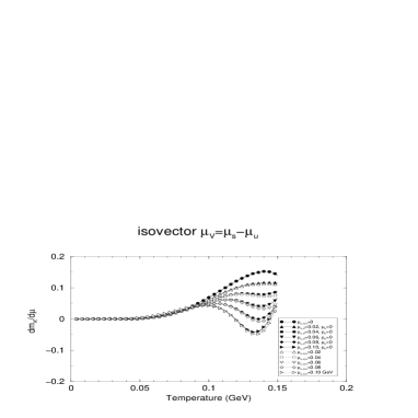
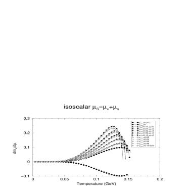
Fig.3 shows ${\partial m_{K}\over\partial\mu_{S}}$ and ${\partial m_{K}\over\partial\mu_{V}}$ at zero and finite chemical potential. It shows that ${\partial m_{K}\over\partial\mu_{S}}$ increases with increasing chemical potential, and there is a critical value between $\mu_{u}$ = $\mu_{s}$ = 0.06 and 0.08 GeV where the sign of ${\partial m_{K}\over\partial\mu_{S}}$ is changed even at below $T_{m_{K}}$. This result is consistent with previous NJL model calculations rs9697 . As in the case of zero chemical potential ${\partial m_{K}\over\partial\mu_{S}}$ changes rapidly near $T_{m_{K}}$. Now, consider the isovector case, where $\mu_{V}=\mu_{s}-\mu_{u}$. Then, one can expect that the sign of ${\partial m_{K}\over\partial\mu_{V}}$ will be opposite to that of ${\partial m_{K}\over\partial\mu_{S}}$ because the $u$ quark plays a dominant role rather than the $s$ quark does. ${\partial m_{K}\over\partial\mu_{V}}$ decreases with increasing chemical potential as shown in the figure.

In Fig. 4 we present ${\partial m_{K}\over\partial\mu_{S}}$ and ${\partial m_{K}\over\partial\mu_{V}}$ for the $K^{+}$. They are obtained by replacing $\omega$ in Eq. (7) with $-\omega$. For comparison we also show ${\partial m_{K}\over\partial\mu_{S}}$ and ${\partial m_{K}\over\partial\mu_{V}}$ for the $K^{-}$ at zero chemical potential.

3. ${\partial m_{\pi}\over\partial\mu}$ in the NJL model

In this section we show ${\partial m_{\pi}\over\partial\mu}$ for the $\pi^{-}$ and $\pi^{+}$. We use the same formulas in the previous section by replacing $m_{s}$, $\mu_{s}$ with $m_{d}$, $\mu_{d}$, respectively. As for the dispersion equation a new coupling strength $G_{\pi}\equiv g_{S}+g_{D}\gamma$ is introduced hk94 .

First, consider the isoscalar $\mu_{S}=\mu_{u}+\mu_{d}$. In the case $m_{u}$ = $m_{d}$, ${\partial m_{\pi}\over\partial\mu_{S}}$ = 0 at zero chemical potential. ${\partial m_{\pi}\over\partial\mu_{S}}$ and ${\partial m_{\pi}\over\partial\mu_{V}}$ for the $\pi^{-}$ and $\pi^{+}$ at finite chemical potential are given in Fig.5. Note that in the case of the isovector chemical potential we take $\mu_{d}$ = 2 $\mu_{u}$.

In the previous calculation we assumed $m_{u}$ = $m_{d}$ = 5.5 MeV. It will be interesting to consider different $u$ and $d$ quark masses, e.g., $m_{u}$ = 4 MeV and $m_{d}$ = 7 MeV. Although the cut-off and the coupling constants should be modified according to this change of the quark masses, we use the same parameters as before and study ${\partial m_{\pi}\over\partial\mu_{S}}$ and ${\partial m_{\pi}\over\partial\mu_{V}}$.

         

Figure 5: ${\partial m_{\pi}\over\partial\mu}$ for the pion with $m_{u}$ = $m_{d}$ = 5.5 MeV.

         

Figure 6: ${\partial m_{\pi}\over\partial\mu}$ for the pion with $m_{u}$ = 4 MeV, $m_{d}$ = 7 MeV.

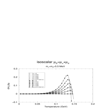
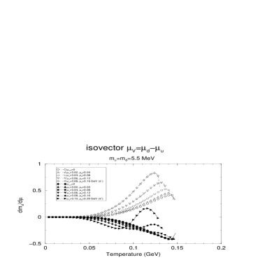
In the case of ${\partial m_{\pi}\over\partial\mu_{S}}$ for the $\pi^{-}$ a transition point appears between $\mu_{u}$ = $\mu_{d}$ = 0.004 GeV and 0.006 GeV as shown in Fig. 6. This transition point seems reasonable considering the mass ratios of $m_{s}/m_{u}$ for the kaon and $m_{d}/m_{u}$ for the pion. For comparison we show both ${\partial m_{\pi}\over\partial\mu_{S}}$ for the $\pi^{-}$ and the $\pi^{+}$. On the other hand, in the case of the isovector chemical potential ${\partial m_{\pi}\over\partial\mu_{V}}$ for the $\pi^{-}$ and $\pi^{+}$ are similar to the previous ones, i.e. the results for the pion with the degenerate $u$ and $d$ quark masses.

4. Discussions

Using the NJL model we have calculated responses of the kaon and pion masses to changes in the chemical potential, ${\partial m_{K}\over\partial\mu}$ and ${\partial m_{\pi}\over\partial\mu}$, at zero and finite chemical potential, and found that ${\partial m\over\partial\mu}$ is much dependent on the mass difference of two quarks, i.e. the mass difference between the $u$ and $s$ (or $d$) quarks.

Let us discuss some uncertainties in our calculations. First, we have considered the Lagrangian (Eq.(1)) without the vector and axial-vector terms. Although there are still arguments about the strength of the vector coupling $g_{V}$ gv , a further analysis including these terms is required. In fact, one of the NJL model calculations showed that the $K^{-}$ mass at finite density with $g_{V}\neq$ 0 is quite different from that with $g_{V}$ = 0 rsp99 . A preliminary result of ${\partial m_{K}\over\partial\mu_{S}}$ for the $K^{-}$ with a non-zero $g_{V}$ also confirms this mc01 .

Second, in the previous section we have also considered the different $u$, $d$ quark masses for the pion ($m_{u}$ = 4 MeV and $m_{d}$ = 7 MeV) and assumed the other parameters are invariant under this change, and found that in the case of ${\partial m_{\pi}\over\partial\mu_{S}}$ the result is slightly different from the previous one, i.e. the pion with the degenerate $u$ and $d$ quark masses ($m_{u}$ = $m_{d}$ = 5.5 MeV). However, we have to take into account variations of the cut-off and coupling constants, although we expect that they would be very small. In the real world, SU(2) symmetry is slightly broken ($m_{u}\neq m_{d}$, $\langle\bar{u}u\rangle\neq\langle\bar{d}d\rangle$), thus a more careful analysis is needed in this case.

Third, in this work we have mainly considered the Case II in hk94 , where only $g_{D}$ has the temperature dependence as shown in Eq.(4). It may be interesting to compare ${\partial m_{K}\over\partial\mu}$ and ${\partial m_{\pi}\over\partial\mu}$ for the Case II with those for the Case I, where all the coupling constants ($g_{S}$, $g_{D}$) and the cut-off $\Lambda$ are independent of temperature and/or chemical potential. We have checked that the behaviors of ${\partial m_{K}\over\partial\mu}$ and ${\partial m_{\pi}\over\partial\mu}$ for the Case I are similar to those for the Case II except for the different Mott temperatures mc01 . This is because $g_{D}$ is rather irrelevant to the pion and kaon masses. However, further analyses including all variations of the cut-off and coupling constants at finite temperature and/or chemical potential are required before any firm conclusions may be drawn.

As a final remark, we find that the second order responses of the kaon and pion masses to the chemical potential, ${\partial^{2}m_{K}\over\partial\mu^{2}}$ and ${\partial^{2}m_{\pi}\over\partial\mu^{2}}$, are much larger than ${\partial m_{K}\over\partial\mu}$ and ${\partial m_{\pi}\over\partial\mu}$, respectively. Thus, one can see rather clearer signals than before.

References

- (1) See, e.g., Proc. of Annual Lattice Conference.
- (2) de Forcrand, Ph., (QCD-TARO Collaboration), Nucl. Phys. B(Proc.Suppl.) 73, 477 (1999); 83, 408 (2000).
- (3) Miyamura, O., talk given at this symposium.
- (4) Nambu, Y. and Jona-Lasinio, G., Phys. Rev. 122, 345 (1961); 124, 246 (1961).
- (5) For a review, see Hatsuda, T. and Kunihiro, T., Phys. Rep. 247, 221 (1994); and references therein.
-
(6)
Gross, D., Pisarski, R.D., and Yaffe, L.G.,
Rev. Mod. Phys. 53, 43 (1981);
Teper, M., Phys. Lett. B202, 553 (1987);
Alkofer, R. and Reinhardt, H., Z. Phys. C45, 275 (1989). -
(7)
Ruivo, M.C. and de Sousa, C.A.,
Phys. Lett. B385, 39 (1996);
de Sousa, C.A. and Ruivo, M.C., Nucl. Phys. A625, 713 (1997). - (8) Ruivo, M.C., de Sousa, C.A., and Providncia, C., Nucl. Phys. A651, 59 (1999).
(9)
Yamawaki, K and Zakharov, V.I., hep-ph/9406373;
Christov, Chr.V., Goeke, K., and Polyakov, M., hep-ph/9501383. - (10) Miyamura, O. and Choe, S., work in preparation.