Probing Flavor Changing Neutrino Interactions Using Neutrino Beams from a Muon Storage Ring

Abstract

We discuss the capabilities of a future neutrino factory based on intense neutrino beams from a muon storage ring to explore the non-standard neutrino matter interactions, which are assumed to be sub-leading effects in the standard mass induced neutrino oscillations. The conjunction of these two mechanisms will magnify fake $CP$ violating effect in the presence of matter which is not coming from the $CP$ phase in the neutrino mixing matrix. We show that such fake $CP$ violation can be observed in neutrino factory experiments by measuring the difference between the neutrino and anti-neutrino probabilities. In order to perform such test, we consider three neutrino flavors, admitting the mixing parameters in the range consistent with the oscillation solution to the atmospheric and the solar neutrino problems, as well as with the constraints imposed by the reactor neutrino data. We show that with a 10 kt detector with 5 years of operation, a stored muon energy $E_{\mu}\geq 20$ GeV, $2\times 10^{20}$ muon decays per year, and a baseline $L\sim 732$ km, such a neutrino facility can probe the non-standard flavor changing neutrino interactions down to the level of ($10^{-3}-10^{-2})~{}G_{F}$, in both $\nu_{\mu}\rightarrow\nu_{\tau}/\bar{\nu}_{\mu}\rightarrow\bar{\nu}_{\tau}$ and $\nu_{e}\rightarrow\nu_{\tau}/\bar{\nu}_{e}\rightarrow\bar{\nu}_{\tau}$ modes.

I Introduction

The atmospheric neutrino experiments [1] present today compelling evidence in favor of $\nu_{\mu}$ disappearance. The solar neutrino experiments [2] as well, are strongly indicating $\nu_{e}$ disappearance. The Los Alamos Liquid Scintillator Neutrino Detector (LSND) [3] has also reported results consistent with neutrino flavor conversion.

The most plausible mechanism of such neutrino flavor disappearance or conversion is the oscillation of neutrino due to quantum interference driven by neutrino mass squared differences $\Delta m^{2}$ [4, 5], which can happen when neutrino flavor eigenstates are supposed to be coherent superpositions of neutrino mass eigenstates [5]. Since the impressive results from the LEP experiments [6, 7], supported recently by the direct observation of $\nu_{\tau}$ by DONUT [8], established that there are at least three active neutrino flavors, it is unavoidable to try to understand such mass induced neutrino oscillations in a full three generation scenario.

Under the assumption of such mass induced neutrino oscillation in three flavor framework, atmospheric neutrino data [9] can be explained by pure $\nu_{\mu}\rightarrow\nu_{\tau}$ oscillations in vacuum [10], though the possibility of having contributions from non-negligible $\nu_{\mu}\rightarrow\nu_{e}$ oscillations is still not discarded [11], even after taking into account the constraints coming from the CHOOZ reactor experiment [12]. On the other hand, solutions to the solar neutrino problem can be provided either by the matter enhanced resonant neutrino conversion, the MSW effect [13, 14], or by vacuum oscillations with a typical wavelength of the order of the Sun-Earth distance [15] with the pure two generation mixing or with small additional participation of a third neutrino on top of the two generation mixing. In this work, we do not take into account signals of the LSND experiment, since simultaneous explanations of the LSND data together with atmospheric as well as solar neutrinos data require the presence of a fourth sterile (electroweak singlet) neutrino, which is beyond the scope of this paper.

Several non-standard (or exotic) explanations of atmospheric as well as solar neutrino data, which do not necessarily invoke neutrino mass and/or mixing, also have been suggested. For atmospheric neutrinos, $\nu_{\mu}$ conversion or disappearance mechanisms induced by neutrino decay [16], flavor changing neutrino interactions [17] and quantum decoherence [18] have been proposed to explain these data. Among them, it was found that the flavor changing solution can not explain well the SK upward going muon data [19] and also it is disfavored by the results coming from K2K [20]. For solar neutrinos, there are also several proposals to explain the data by invoking non-standard neutrino properties such as magnetic moment [21], non-standard neutrino interactions [22] or even by a tiny violation of the equivalence principle [23].

While some of these non-standard solutions can explain quite well the data, it is generally believed that the most plausible solutions are provided by the standard mass induced oscillation mechanism, because mass and mixing are the simplest extension of the standard model and moreover, it is the unique mechanism which can explain well both atmospheric and solar neutrino observations at the same time, without additional neutrino properties.

However, even in this case, we consider that it is quite possible that some non-standard neutrino properties could induce some sub-leading effect in addition to the the standard mass induced neutrino oscillation without causing any inconsistency with the present observations. We are particularly interested in such sub-leading effects induced by flavor changing neutrino interactions. These type of interactions were first suggested in Ref. [24], and then discussed as a possible mechanism to solve the solar neutrino problem in Ref. [25, 26].

Indeed, many models of neutrino mass [27, 28, 29] are also a natural source of non-standard neutrino matter interactions (NSNI) which can be, phenomenologically, classified into two types : flavor changing neutrino interactions (FCNI) and flavor diagonal neutrino interactions (FDNI), as we will discuss in detail in our work.

Therefore, we believe that even if mass induced oscillations really take place in nature and such NSNI are not playing any relevant roles in explaining the observed neutrino data, it could be important to study NSNI interactions as secondary contributions, in order to gain some handle on new physics beyond the electroweak standard model. The crucial point of our idea is to use the fact that the simultaneous presence of neutrino masses and NSNI can enhance the difference in the conversion probabilities between neutrino and anti-neutrino channels in matter causing fake $CP$ violation [30].

Our aim here is to test such interactions in a future neutrino factory. A neutrino factory [31], which could be a milestone for a future muon-collider project, presents a possibility to go beyond the goal of measuring with great precision the oscillation parameters. It will offer us the chance to measure separately the oscillating probabilities in $CP$-conjugate channels, such as $\nu_{\mu}\rightarrow\nu_{e},\nu_{\tau}$ and $\bar{\nu}_{\mu}\rightarrow\bar{\nu}_{e},\bar{\nu}_{\tau}$, with high intensity neutrino beams produced by a muon storage ring [31], after neutrinos travel through several hundreds of kilometers in the Earth mantle before reaching the detector.

There are already quite a few very interesting studies that have shown the prospects of neutrino factories to measure the mixing parameters and obtaining the pattern of neutrino masses [31, 32, 33], to test matter effects [32, 33], $CP$ violation in the leptonic sector [34, 35], $CPT$-odd interactions [36] and distinguish the mass induced solution for the atmospheric neutrino anomaly from the decoherence one [37], or possible neutrino oscillation induced by violation of the equivalence principle [38]. Signals of $R-$parity violating supersymmetric interactions which can be mistaken for neutrino oscillations in neutrino factory experiments were also investigated in Ref. [39], where it is found that these novel contributions basically do not affect the $\tau$ event rate for baselines greater than 200 km, except if the new couplings are close to their perturbative limit.

Here, we investigate the capacity of neutrino factory experiments to probe neutrino oscillations beyond the standard mechanism assuming mixing parameters compatible with atmospheric, solar and reactor neutrino experiments and by so doing to discover new physics or put restrictive limits on NSNI models. Our results will be presented as a function of the distance between source and detector for two particular muon energies.

In Sec. II, we define the formalism that will be used throughout this paper. In Sec. III, we describe the various experimental set-ups we will consider, as well as the details of our experimental simulations. In Sec. IV, we show our predictions for the $\nu_{\mu}\rightarrow\nu_{\tau}$ and $\nu_{e}\rightarrow\nu_{\tau}$ channels with and without $CP$ violation. Finally in Sec. V, we discuss our results and present our conclusions.

II Modified Oscillation Formalism with NSNI

There are currently several experimental bounds on NSNI coming from the non-observation of lepton flavor violating process [6], from violation of lepton flavor universality, or from neutrino scattering data. Model independent analysis of these experimental constraints derived from $SU(2)_{L}$ related interactions, that can be found in Refs. [40, 22], in general, gives stronger bound for $\nu_{e}-\nu_{\mu}$ channel, typically set the maximal strength of NSNI normalized by the electro weak interactions strength, i.e. $G_{F}$, to be at the level much smaller than one-percent whereas the bounds for $\nu_{\mu}-\nu_{\tau}$ and $\nu_{e}-\nu_{\tau}$ channels are substantially weaker typically at the level of $\sim 10^{-2}-10^{-1}$ in unit of $G_{F}$. Therefore, in this work, we will only consider the two channels $\nu_{\mu}-\nu_{\tau}$, $\nu_{e}-\nu_{\tau}$ and their anti-neutrino ones, which are less constrained from the laboratory experiments.

In the usual three generation neutrino oscillation framework, we can define the correspondence between neutrino mass eigenstates and neutrino interaction eigenstates by,

$$\left[\begin{array}[]{c}\nu_{e}\\ \nu_{\mu}\\ \nu_{\tau}\end{array}\right]=U\left[\begin{array}[]{c}\nu_{1}\\ \nu_{2}\\ \nu_{3}\end{array}\right],$$ (1)

where $\nu_{i}$ ($i=1,2,3$) are the neutrino mass eigenstates, and $\nu_{\alpha}$ ($\alpha=e,\mu,\tau$) are the neutrino flavor eigenstates with the standard parameterization for Maki-Nakagawa-Sakata [5] mixing matrix $U$ given by,

$$U=\left[\begin{array}[]{ccc}c_{12}c_{13}&s_{12}c_{13}&s_{13}e^{-i\delta}\\ -s_{12}c_{23}-c_{12}s_{23}s_{13}e^{i\delta}&c_{12}c_{23}-s_{12}s_{23}s_{13}e^{i\delta}&s_{23}c_{13}\\ s_{12}s_{23}-c_{12}c_{23}s_{13}e^{i\delta}&-c_{12}s_{23}-s_{12}c_{23}s_{13}e^{i\delta}&c_{23}c_{13}\end{array}\right],$$ (2)

where $c_{ij}$ and $s_{ij}$ denote the cosine and the sine of $\theta_{ij}$ and $\delta$ is the $CP$ violating phase.

A NSNI in $\nu_{\mu}\rightarrow\nu_{\tau}$ channel

If we consider the possibility of NSNI only in the $\nu_{\mu}\rightarrow\nu_{\tau}$ channel, the evolution Hamiltonian in matter has the form,

$$i{\displaystyle\frac{d}{dr}}\left(\begin{array}[]{c}\nu_{e}\\ \nu_{\mu}\\ \nu_{\tau}\end{array}\right)=\left[U\left(\begin{array}[]{ccc}0&0&0\\ 0&\Delta_{21}&0\\ 0&0&\Delta_{31}\end{array}\right)U^{\dagger}+\left(\begin{array}[]{ccc}V_{e}(r)&0&0\\ 0&0&\epsilon^{f}_{\mu\tau}V_{f}(r)\\ 0&\epsilon^{f}_{\mu\tau}V_{f}(r)&\epsilon^{\prime f}_{\mu\tau}V_{f}(r)\end{array}\right)\right]\left(\begin{array}[]{c}\nu_{e}\\ \nu_{\mu}\\ \nu_{\tau}\end{array}\right),$$ (3)

where $\Delta_{ij}=\Delta m^{2}_{ij}/2E=(m^{2}_{i}-m^{2}_{j})/2E,\,i,j=1,2,3$, $E$ is the neutrino energy, $V_{f}(r)=\sqrt{2}\,G_{F}n_{f}(r),f=u,d,e$, $V_{f}(r)\epsilon^{f}_{\mu\tau}$ is the flavor-changing $\nu_{\mu}+f\rightarrow\nu_{\tau}+f$ forward scattering amplitude with the interacting fermion $f$ (electron, $d$ or $u$ quark) and $V_{f}(r)\epsilon_{\mu\tau}^{\prime f}$ is the difference between the flavor diagonal $\nu_{\mu}-f$ and $\nu_{\tau}-f$ elastic forward scattering amplitudes, with $n_{f}(r)$ being the number density of the fermions which induce such processes. In the evolution Eq. (3), $\epsilon^{f}_{\mu\tau}$ and $\epsilon^{\prime f}_{\mu\tau}$ are the phenomenological parameters which characterize the strength of FCNI and FDNI, respectively. The fermion number density $n_{f}(r)$ can be written in terms of the matter density $\rho$ as $n_{f}(r)=\rho(r)Y_{f}$, where $Y_{f}$ is the fraction of the fermion $f$ per nucleon, $\sim 1/2$ for electrons and $\sim 3/2$ for $u$ or $d$ quarks. In all cases, electron neutrinos will coherently scatter off the electrons present in matter through the standard electroweak charged currents which introduce non trivial contributions to the neutrino evolution equations. These contributions are taken into account by the diagonal term $V_{e}(r)$ in Eq. (3).

A similar form applies to the evolution of anti-neutrinos except that $V_{e,f}(r)\rightarrow-V_{e,f}(r)$ and $U\rightarrow U^{*}$. We assume the density profile of the Earth to be the one given by the Preliminary Reference Earth Model [41] and solve these evolution equations numerically to compute the oscillation probabilities $P(\nu_{\mu}\rightarrow\nu_{\tau})$ and $P(\bar{\nu}_{\mu}\rightarrow\bar{\nu}_{\tau})$.

B NSNI in $\nu_{e}\rightarrow\nu_{\tau}$ channel

Now, if we consider NSNI only in the $\nu_{e}\rightarrow\nu_{\tau}$ channel, the evolution Hamiltonian in matter will have the form,

$$i{\displaystyle\frac{d}{dr}}\left(\begin{array}[]{c}\nu_{e}\\ \nu_{\mu}\\ \nu_{\tau}\end{array}\right)=\left[U\left(\begin{array}[]{ccc}0&0&0\\ 0&\Delta_{21}&0\\ 0&0&\Delta_{31}\end{array}\right)U^{\dagger}+\left(\begin{array}[]{ccc}V_{e}(r)&0&\epsilon^{f}_{e\tau}V_{f}(r)\\ 0&0&0\\ \epsilon^{f}_{e\tau}V_{f}(r)&0&\epsilon^{\prime f}_{e\tau}V_{f}(r)\end{array}\right)\right]\left(\begin{array}[]{c}\nu_{e}\\ \nu_{\mu}\\ \nu_{\tau}\end{array}\right).$$ (4)

Again for anti-neutrinos we have to make the following substitution $V_{e,f}(r)\rightarrow-V_{e,f}(r)$ and $U\rightarrow U^{*}$. We obtain the oscillation probabilities $P(\nu_{e}\rightarrow\nu_{\tau})$ and $P(\bar{\nu}_{e}\rightarrow\bar{\nu}_{\tau})$ by numerically solving Eq. (4) for neutrinos and the corresponding modified one for anti-neutrinos.

In the following, we will drop the $f$ superscript of $\epsilon$, $\epsilon^{\prime}$ and consider interactions only with either $u$ or $d$ quarks, since limits on interactions with electrons can be obtained by a simple re-scale of our plots. If NSNI are caused by electrons, $\epsilon$ and $\epsilon^{\prime}$ parameters must be increased by a factor 3 to get the same effect presented in this paper.

C Useful Two Generation Formulae

It is instructive to write down the analytical expression for the conversion probability in two generation considering constant matter density. This will help to understand the full-fledged three generation numerical results. The probability of $\nu_{\alpha}\rightarrow\nu_{\tau}$, $\alpha=e,\mu$, conversion can be written as

$$P(\nu_{\alpha}\rightarrow\nu_{\tau}) = \displaystyle\frac{4\left(\displaystyle\frac{\Delta}{2}\sin 2\theta+\epsilon_{\alpha\tau}V_{f}\right)^{2}}{4(\displaystyle\frac{\Delta}{2}\sin 2\theta+\epsilon_{\alpha\tau}V_{f})^{2}+(\Delta\cos 2\theta+\epsilon^{\prime}_{\alpha\tau}V_{f}-\delta_{e\alpha}V_{e})^{2}}$$ (6)

$$\displaystyle\times\sin^{2}\left\{\frac{L}{2}\left[4(\frac{\Delta}{2}\sin 2\theta+\epsilon_{\alpha\tau}V_{f})^{2}+(\Delta\cos 2\theta+\epsilon^{\prime}_{\alpha\tau}V_{f}-\delta_{e\alpha}V_{e})^{2}\right]^{1\over 2}\right\},$$

where $\Delta$ and $\sin 2\theta$ will be chosen depending on the oscillation mode. The probability of $\bar{\nu}_{\alpha}\rightarrow\bar{\nu}_{\tau}$ conversion is analogous to the above except that $V_{e,f}\rightarrow-V_{e,f}$.

One can easily see that the probability is much more sensitive to $\epsilon_{\alpha\tau}$ than to $\epsilon^{\prime}_{\alpha\tau}$, since $\epsilon_{\alpha\tau}$ appears in the numerator and in the denominator of the amplitude in Eq. (6), while $\epsilon^{\prime}_{\alpha\tau}$ appears only in the denominator. Moreover, the terms involving $\epsilon_{\alpha\tau}$ are increased by a factor 4 with respect to the terms involving $\epsilon^{\prime}_{\alpha\tau}$. These features become more prominent if the distance is not so large and the contribution from FCNI are small as we will see below.

Let us take some typical values for the mixing parameters and the neutrino energy we are going to consider in this work, $\Delta m^{2}\sim\text{few}\times 10^{-3}$ eV², $E$ = few $\times 10$ GeV and not very large distance, $L\mathrel{\raise 1.29167pt\hbox{$<$\kern-7.5pt\lower 4.30554pt\hbox{$\sim$}}}1000$ km. In this case, taking the NSNI effects to be small, i.e. , $\epsilon,\epsilon^{\prime}\ll 1$, the probability in Eq. (6) can be approximated, up to the first order in the NSNI parameters, as follows,

$$P(\nu_{\alpha}\rightarrow\nu_{\tau})\simeq\frac{1}{4}\Delta\sin 2\theta\displaystyle\left(\Delta\sin 2\theta+4~{}\epsilon_{\alpha\tau}V_{f}\right)L^{2}.$$ (7)

Note that there is no dependence on the $\epsilon^{\prime}_{\alpha\tau}$ parameter in the above probability. For the corresponding anti-neutrino channel, $V_{f}$ must be replaced by $-V_{f}$ in Eq. (7), which lead to a different probability. It is important to point out that, as we can see from Eq. (6), only the presence of NSNI term alone without neutrino mass ($\Delta\rightarrow 0$) can not cause the neutrino and anti-neutrino probabilities to differ.

In order to extract the information on NSNI, without knowing the very precise values of mixing parameters, we must compare in some way, the probability for neutrinos and anti-neutrinos. In this work, we consider the ratio of the expected number of events for anti-neutrinos and neutrinos, which can be approximately inferred, for small values of $\epsilon_{\alpha\tau}$ taking into account the difference in the detection cross sections ($\sigma_{\bar{\nu}_{\tau}}$ and $\sigma_{\nu_{\tau}}$), from the simple expression,

$$R(P) \equiv \frac{\sigma_{\bar{\nu}_{\tau}}P(\bar{\nu}_{\alpha}\rightarrow\bar{\nu}_{\tau})}{\sigma_{\nu_{\tau}}P(\nu_{\alpha}\rightarrow\nu_{\tau})}\simeq{1\over 2}-\frac{4~{}\epsilon_{\alpha\tau}V_{f}}{\Delta\sin 2\theta+4~{}\epsilon_{\alpha\tau}V_{f}}.$$ (8)

From the expressions in Eqs. (7) and (8), it is clear that the oscillation probabilities are much more sensitive to the FCNI parameter, $\epsilon_{\alpha\tau}$, than to the FDNI parameter, $\epsilon^{\prime}_{\alpha\tau}$, and moreover, in the ratio, the FCNI effect does not depend on the distance as long as it is not very large, i.e. $L\mathrel{\raise 1.29167pt\hbox{$<$\kern-7.5pt\lower 4.30554pt\hbox{$\sim$}}}1000$ km, this will be confirmed in the following sections.

In this work, we assume that $\Delta m^{2}_{31}$ is positive and do not consider the negative case (inverted hierarchy) because such case will covered as we consider both the positive and negative sign of $\epsilon_{\alpha\tau}$. ¿From Eq. (8) we can see that the same effect is obtained when $(\Delta m^{2}_{31},\epsilon_{\alpha\tau})$ is replaced by $(-\Delta m^{2}_{31},-\epsilon_{\alpha\tau})$, which is valid as long as $L\mathrel{\raise 1.29167pt\hbox{$<$\kern-7.5pt\lower 4.30554pt\hbox{$\sim$}}}1000$ km.

III Experimental Set-up and Observables

Many authors [31] have emphasized the advantages of using the long straight section of a high intensity muon storage ring to make a neutrino factory. The muons (anti-muons) accelerated to an energy $E_{\mu}$ constitute a pure source of both $\nu_{\mu}$ ($\bar{\nu}_{\mu}$) and $\bar{\nu}_{e}$ ($\nu_{e}$) through their decay $\mu^{-}\rightarrow e^{-}\bar{\nu}_{e}\nu_{\mu}$ ($\mu^{+}\rightarrow e^{+}\nu_{e}\bar{\nu}_{\mu}$) with well known initial flux and energy distribution. In this context it is quite suitable to perform very precise measurements of the probability of oscillation in $CP$-conjugated channels, such as $\nu_{\mu}\rightarrow\nu_{\tau}$ and $\bar{\nu}_{\mu}\rightarrow\bar{\nu}_{\tau}$ or $\nu_{e}\rightarrow\nu_{\tau}$ and $\bar{\nu}_{e}\rightarrow\bar{\nu}_{\tau}$.

There are many propositions for these type of Neutrino Factories, with values for the energy of the stored muon (anti-muon), $E_{\mu}$, going from 10 GeV to 250 GeV, for baselines, $L$, ranging from 730 km to 10  000 km, in any case the neutrino beam penetrating a fair bit of the Earth’s crust. Since we do not know which will be the final configuration we will do our estimations for several possible configurations. We do our calculations taking into account all the available relevant experimental information to compute real experimental observables.

Here we will explore the neutrino factory as an appearance $\nu_{\tau}$ ($\bar{\nu}_{\tau}$) experiment. We define the following observables of interest:

$$R_{\mu\tau}(\epsilon_{\mu\tau},\epsilon^{\prime}_{\mu\tau})=\frac{N^{+}_{\bar{\nu}_{\tau}}(\epsilon_{\mu\tau},\epsilon^{\prime}_{\mu\tau})}{N_{\nu_{\tau}}^{-}(\epsilon_{\mu\tau},\epsilon^{\prime}_{\mu\tau})},$$ (9)

and

$$R_{e\tau}(\epsilon_{e\tau},\epsilon^{\prime}_{e\tau})=\frac{N^{-}_{\bar{\nu}_{\tau}}(\epsilon_{e\tau},\epsilon^{\prime}_{e\tau})}{N^{+}_{\nu_{\tau}}(\epsilon_{e\tau},\epsilon^{\prime}_{e\tau})},$$ (10)

where $R_{\mu\tau}$ ($R_{e\tau}$) is the ratio between the total number of detectable $\bar{\nu}_{\tau}$-events, $N^{+}_{\bar{\nu}_{\tau}}$ ($N^{-}_{\bar{\nu}_{\tau}}$), when the neutrino beam is made of $\mu^{+}$ ($\mu^{-}$) decays, in the $\bar{\nu}_{\mu}\rightarrow\bar{\nu}_{\tau}$ ($\bar{\nu}_{e}\rightarrow\bar{\nu}_{\tau}$) channel, over the total number of detectable $\nu_{\tau}$-events, $N^{-}_{\nu_{\tau}}$ ($N^{+}_{\nu_{\tau}}$), when the beam is made of $\mu^{-}$ ($\mu^{+}$) decays, in the $\nu_{\mu}\rightarrow\nu_{\tau}$ ($\nu_{e}\rightarrow\nu_{\tau}$) channel. These numbers can be calculated as

$$N^{-}_{\nu_{\tau}}(\epsilon_{\mu\tau},\epsilon^{\prime}_{\mu\tau})=n_{\mu^{-}}M\frac{10^{9}N_{\text{A}}}{m^{2}_{\mu}\pi}\frac{E^{3}_{\mu}}{L^{2}}\int_{E_{\text{th}}}^{E_{\mu}}h(E)P(\nu_{\mu}\rightarrow\nu_{\tau})(E)dE,$$ (11)

$$N^{+}_{\bar{\nu}_{\tau}}(\epsilon_{\mu\tau},\epsilon^{\prime}_{\mu\tau})=n_{\mu^{+}}M\frac{10^{9}N_{\text{A}}}{m^{2}_{\mu}\pi}\frac{E^{3}_{\mu}}{L^{2}}\int_{E_{\text{th}}}^{E_{\mu}}\bar{h}(E)P(\bar{\nu}_{\mu}\rightarrow\bar{\nu}_{\tau})(E)dE,$$ (12)

$$N^{+}_{\nu_{\tau}}(\epsilon_{e\tau},\epsilon^{\prime}_{e\tau})=n_{\mu^{-}}M\frac{10^{9}N_{\text{A}}}{m^{2}_{\mu}\pi}\frac{E^{3}_{\mu}}{L^{2}}\int_{E_{\text{th}}}^{E_{\mu}}g(E)P(\nu_{e}\rightarrow\nu_{\tau})(E)dE,$$ (13)

$$N^{-}_{\bar{\nu}_{\tau}}(\epsilon_{e\tau},\epsilon^{\prime}_{e\tau})=n_{\mu^{+}}M\frac{10^{9}N_{\text{A}}}{m^{2}_{\mu}\pi}\frac{E^{3}_{\mu}}{L^{2}}\int_{E_{\text{th}}}^{E_{\mu}}\bar{g}(E)P(\bar{\nu}_{e}\rightarrow\bar{\nu}_{\tau})(E)dE,$$ (14)

with

$$h(E)= \displaystyle 2\frac{E^{2}}{E_{\mu}^{2}}(3-2\frac{E}{E_{\mu}})\frac{\sigma_{\nu_{\tau}}(E)}{E_{\mu}^{2}}\eta_{\tau}(E),$$ (15)

$$\bar{h}(E)= \displaystyle 2\frac{E^{2}}{E_{\mu}^{2}}(3-2\frac{E}{E_{\mu}})\frac{\sigma_{\nu_{\bar{\tau}}}(E)}{E_{\mu}^{2}}\,\eta_{\bar{\tau}}(E),$$ (16)

$$g(E)= \displaystyle 12\frac{E^{2}}{E_{\mu}^{2}}(1-\frac{E}{E_{\mu}})\frac{\sigma_{\nu_{\tau}}(E)}{E_{\mu}^{2}}\eta_{\tau}(E),$$ (17)

$$\bar{g}(E)= \displaystyle 12\frac{E^{2}}{E_{\mu}^{2}}(1-\frac{E}{E_{\mu}})\frac{\sigma_{\nu_{\bar{\tau}}}(E)}{E_{\mu}^{2}}\,\eta_{\bar{\tau}}(E),$$ (18)

where $E_{\mu}$ is the muon source energy, $M$ is the detector mass in ktons, $n_{\mu^{-}}$ and $n_{\mu^{+}}$ the number of useful $\mu^{-}$ and $\mu^{+}$ decays, respectively, $10^{9}N_{\text{A}}$ is the number of nucleons in a kton and $m_{\mu}$ is the mass of the muon. The functions $h(E)$ and $\bar{h}(E)$ ($g(E)$ and $\bar{g}(E)$), contain the $\nu_{\mu}$ and $\bar{\nu}_{\mu}$ ($\nu_{e}$ and $\bar{\nu}_{e}$) energy spectrum normalized to 1, the charged current interaction cross section for $\nu_{\tau}$ and $\bar{\nu}_{\tau}$ [42], and the $\nu_{\tau}$, $\bar{\nu}_{\tau}$ detection efficiencies $\eta_{\tau}$,$\eta_{\bar{\tau}}$, respectively.

We have used $E_{\text{th}}=4$ GeV and assumed, for simplicity, that once this cut is applied the tau neutrino and tau anti-neutrino, can be observed with the same efficiency $\eta_{\tau}=\eta_{\bar{\tau}}=0.33$ which seems to be achievable by means of exploiting one-prong and three-prong $\tau$ decay topologies along with displaced vertex or kinks resulting from $\tau$-lepton decays [43]. We have neglected the finite detector resolution following Ref. [32].

In our study we will consider the following general characteristics for the neutrino factory : $E_{\mu}=20$ GeV and 50 GeV, $2\times 10^{20}$ muon decays, a 10 kton detector and 5 years of data taking. We would like to point out that the observable $R_{\mu\tau}$ ($R_{e\tau}$) can amplify the differences between $N^{-}_{\nu_{\tau}}(N^{+}_{\nu_{\tau}})$ and $N^{+}_{\bar{\nu}_{\tau}}(N^{-}_{\bar{\nu}_{\tau}})$, independent of the absolute number of events.

IV Perspective of Future Neutrino Factories

In order to estimate the maximal limit on $\epsilon_{\alpha\tau}$ and $\epsilon^{\prime}_{\alpha\tau}$, with $\alpha=e,\mu$ that can be achieved by a neutrino factory we define the following functions

$$\chi^{2}(\epsilon_{\alpha\tau},\epsilon^{\prime}_{\alpha\tau}) = 2[N^{\pm}_{\nu_{\tau}}(\epsilon_{\alpha\tau},\epsilon^{\prime}_{\alpha\tau})-N^{\pm}_{\nu_{\tau}}(\epsilon_{\alpha\tau}=0,\epsilon^{\prime}_{\alpha\tau}=0)]$$ (20)

$$+ 2N^{\pm}_{\nu_{\tau}}(\epsilon_{\alpha\tau}=0,\epsilon^{\prime}_{\alpha\tau}=0)\;\ln\left(\frac{N^{\pm}_{\nu_{\tau}}(\epsilon_{\alpha\tau}=0,\epsilon^{\prime}_{\alpha\tau}=0)}{N^{\pm}_{\nu_{\tau}}(\epsilon_{\alpha\tau},\epsilon^{\prime}_{\alpha\tau})}\right),$$ (21)

and

$$\bar{\chi}^{2}(\epsilon_{\alpha\tau},\epsilon^{\prime}_{\alpha\tau}) = 2[N^{\mp}_{\bar{\nu}_{\tau}}(\epsilon_{\alpha\tau},\epsilon^{\prime}_{\alpha\tau})-N^{\mp}_{\nu_{\tau}}(\epsilon_{\alpha\tau}=0,\epsilon^{\prime}_{\alpha\tau}=0)]$$ (22)

$$+ 2N^{\mp}_{\bar{\nu}_{\tau}}(\epsilon_{\alpha\tau}=0,\epsilon^{\prime}_{\alpha\tau}=0)\;\ln\left(\frac{N^{\mp}_{\bar{\nu}_{\tau}}(\epsilon_{\alpha\tau}=0,\epsilon^{\prime}_{\alpha\tau}=0)}{N^{\mp}_{\bar{\nu}_{\tau}}(\epsilon_{\alpha\tau},\epsilon^{\prime}_{\alpha\tau})}\right),$$ (23)

so that for fixed values of the oscillation parameters, one can compute the number of standard deviations of separation between pure mass induced oscillation and mass induced oscillation plus NSNI contribution as a function of $\epsilon_{\alpha\tau}$ and $\epsilon^{\prime}_{\alpha\tau}$, as $n_{\sigma}=\sqrt{(\chi^{2}+\bar{\chi}^{2})/2}$.

We will consider in our analyses the following range for the oscillation parameters : $1\times 10^{-3}$ eV² $\mathrel{\raise 1.29167pt\hbox{$<$\kern-7.5pt\lower 4.30554pt\hbox{$\sim$}}}$ $|\Delta m^{2}_{31}|\mathrel{\raise 1.29167pt\hbox{$<$\kern-7.5pt\lower 4.30554pt\hbox{$\sim$}}}7\times 10^{-3}$ eV², $|\Delta m^{2}_{21}|\mathrel{\raise 1.29167pt\hbox{$<$\kern-7.5pt\lower 4.30554pt\hbox{$\sim$}}}1\times 10^{-3}$ eV², $0.8\mathrel{\raise 1.29167pt\hbox{$<$\kern-7.5pt\lower 4.30554pt\hbox{$\sim$}}}\sin^{2}2\theta_{23}\mathrel{\raise 1.29167pt\hbox{$<$\kern-7.5pt\lower 4.30554pt\hbox{$\sim$}}}1.0$, $0.7\mathrel{\raise 1.29167pt\hbox{$<$\kern-7.5pt\lower 4.30554pt\hbox{$\sim$}}}\sin^{2}2\theta_{12}\mathrel{\raise 1.29167pt\hbox{$<$\kern-7.5pt\lower 4.30554pt\hbox{$\sim$}}}1.0$ and $\sin^{2}2\theta_{13}\mathrel{\raise 1.29167pt\hbox{$<$\kern-7.5pt\lower 4.30554pt\hbox{$\sim$}}}0.3$; with $0\leq\theta_{12},\theta_{23},\theta_{13}<\pi/2$ and $0\leq\delta\leq\pi/2$. To the extent that the contributions from the sub-leading solar $|\Delta m^{2}_{21}|<<|\Delta m^{2}_{31}|$ scale are small, our results apply approximately to other solar scenarios.

A NSNI in $\nu_{\mu}\rightarrow\nu_{\tau}$ channel

The interesting feature of this channel is not only that for the standard oscillation mechanism, with $\delta=0$, the fake $CP$ violation induced by matter effect is very small [44], under our assumptions about the mixing parameters, but also that even if we consider the $CP$ violation phase to be maximal ($\delta=\pi/2$), this quantity remains quite negligible. This is due to the fact that $\sin^{2}2\theta_{13}$ is highly constrained by CHOOZ and the atmospheric neutrino data. On the other hand, as we have seen in Sec. II the inclusion of an extra contributions from NSNI in the neutrino evolution Hamiltonian will enhance the fake $CP$ violation in matter.

To illustrate the size of the effect due to NSNI in this channel we plot in Fig. 1 and 2 the ratio $R_{\mu\tau}$ as a function of $L$ for $E_{\mu}=20$ and 50 GeV respectively, for $\epsilon^{\prime}_{\mu\tau}=0$ and $\epsilon_{\mu\tau}=0.001$ and 0.01. These plots were done for the best fit values of the oscillation parameters for the combined analysis of atmospheric, solar and reactor data according to Ref. [45], assuming the large mixing angle solution to the solar neutrino anomaly, i.e. , $\Delta m^{2}_{31}=3.1\times 10^{-3}$ eV², $\Delta m^{2}_{21}=3.3\times 10^{-5}$ eV², $\sin^{2}2\theta_{23}=0.97$, $\sin^{2}2\theta_{12}=0.78$ and $\sin^{2}2\theta_{13}=0.02$, with $\delta=0$.

For no NSNI, the ratio is nearly constant around 0.5, it is essentially dominated by the ratio between $\nu_{\tau}$ and $\bar{\nu}_{\tau}$ cross sections since the standard matter effect is negligible ($P(\nu_{\mu}\rightarrow\nu_{\tau})\approx P(\bar{\nu}_{\mu}\rightarrow\bar{\nu}_{\tau})$) . As FCNI are introduced by increasing the value of $\epsilon_{\mu\tau}$, we observe the effect of the new interactions pop in, becoming quite appreciable for $\epsilon_{\mu\tau}\sim 10^{-2}$ and stronger as we increase in energy. This dependence in energy can be easily understood using the two generation formula given in Eqs. (6)-(8), setting $\Delta=\Delta_{32}$ and $\sin 2\theta=\sin 2\theta_{23}$. Although we are here working in a full three generation scheme, this approach will be good enough to interpret the general behavior of the probabilities. This is because these two parameters are the leading parameters for conversion in this channel in the three generation framework. ¿From Eqs. (7) and (8), we see that the effect of fake $CP$ violation become larger as energy grows and can reach smaller values of $\epsilon_{\mu\tau}$.

Note that the impact of using the Earth’s density profile can be appreciated in the small distortions of the curves for $L>1000$ km, which is specially sizable in Fig. 2, for $\epsilon_{\mu\tau}$ =0.01, which also can be explained in first approximation by the two generation formula.

For our statistical analyses of the limits that can be achieved by a neutrino factory, we have chosen to work with $L=$ 732 km. Two reasons support this choice : the FCNI effect is stronger and independent of $L$ up to 1000 km (which can be understood from Eq. (8) in Sec. II C) and this baseline is compatible with the CERN-Gran Sasso or Fermilab-Soudan distance. Besides this at 732 km the neutrino flux is still quite big.

In Figs. 3 and 4, we show the region of sensitivity in $|\epsilon^{\prime}_{\mu\tau}|\times|\epsilon_{\mu\tau}|$ plane for $\epsilon^{\prime}_{\mu\tau},\epsilon_{\mu\tau}>0$ computed using the prescription given in Sec. IV and requiring a $n_{\sigma}=3,5$ separation. We plot the maximal limit for two extreme cases, one for $\Delta m^{2}_{32}=1\times 10^{-3}$ eV² and the other for $\Delta m^{2}_{32}=7\times 10^{-3}$ eV². To give an idea of the corresponding number of events expected at the limiting points, we give in Tab. I these numbers for $\epsilon^{\prime}_{\mu\tau}=0$. We have checked that these results are not modified by changes in the values of the other oscillation parameters or by the adopted sign of $\Delta m^{2}_{32}$ or of $\Delta m^{2}_{21}$. In particular, $P(\nu_{\mu}\rightarrow\nu_{\tau})$ and the $P(\bar{\nu}_{\mu}\rightarrow\bar{\nu}_{\tau})$ are essentially independent of $\delta$ and the value of $\Delta m^{2}_{21}$. We also have done the same calculation in the case of either $\epsilon^{\prime}_{\mu\tau}<0$ or $\epsilon_{\mu\tau}<0$ or both, but we do not show these curves here since they are almost identical to the ones in Figs. 3 and 4.

For $E_{\mu}=$ 20 GeV we see that it is possible to probe, at 3 $\sigma$ level, $|\epsilon_{\mu\tau}|\mathrel{\raise 1.29167pt\hbox{$>$\kern-7.5pt\lower 4.30554pt\hbox{$\sim$}}}6\times 10^{-3}$ and $|\epsilon^{\prime}_{\mu\tau}|\mathrel{\raise 1.29167pt\hbox{$>$\kern-7.5pt\lower 4.30554pt\hbox{$\sim$}}}1.7~{}(0.6)$, for $E_{\mu}=$ 50 GeV, $|\epsilon_{\mu\tau}|\mathrel{\raise 1.29167pt\hbox{$>$\kern-7.5pt\lower 4.30554pt\hbox{$\sim$}}}1.6\times 10^{-3}$ and $|\epsilon^{\prime}_{\mu\tau}|\mathrel{\raise 1.29167pt\hbox{$>$\kern-7.5pt\lower 4.30554pt\hbox{$\sim$}}}1.4~{}(0.4)$, for $\Delta m^{2}_{32}=1\times 10^{-3}$ eV² ($7\times 10^{-3}$ eV²). As explained in Sec. IV we did not expect to be very sensitive to $\epsilon^{\prime}_{\mu\tau}$, also the limits are better at 50 GeV due to the flux increase with $E_{\mu}^{3}$.

Finally we note that, although the oscillation probabilities in this channel can get quite large, the difference in the neutrino and anti-neutrino probabilities remains small, unless $|\epsilon_{\mu\tau}|\rightarrow 1$. This means that the constraints relies mainly on a large event statistics.

B NSNI in $\nu_{e}\rightarrow\nu_{\tau}$ channel

We plot in Figs. 5 and 6 the ratio $R_{e\tau}$ as a function of $L$ for $E_{\mu}=$ 20 GeV and 50 GeV, respectively, for $\epsilon^{\prime}_{e\tau}=0$ and $\epsilon_{e\tau}=0.0001,0.001$ and 0.01. We can compare these figures with Figs. 1 and 2 for $R_{\mu\tau}$ and make two observation. First, for the case without NSNI we have a strong deviation in the channel $\nu_{e}\rightarrow\nu_{\tau}$ from the value 0.5 after $L\mathrel{\raise 1.29167pt\hbox{$>$\kern-7.5pt\lower 4.30554pt\hbox{$\sim$}}}1000$ km, this is because matter effects ($V_{e}$) are specially important in this mode, in contrast with $\nu_{\mu}\rightarrow\nu_{\tau}$ where they are small. Second, when we add the non-standard contributions the effect in $\nu_{e}\rightarrow\nu_{\tau}$ channel is again more relevant than for $\nu_{\mu}\rightarrow\nu_{\tau}$. This can be understood since at first approximation we can think that the modified three generation probabilities $P(\nu_{e}\rightarrow\nu_{\tau})$ and $P(\bar{\nu}_{e}\rightarrow\bar{\nu}_{\tau})$, as it is the case for the standard ones [33], must be proportional to $\sin^{2}2\theta_{13}^{m}$ in matter, only in our case we also have to consider the contributions of the non-standard interactions. This permits a qualitative understanding of our results in terms of the two-generation formula (Eq. (6)) replacing $\Delta$ by $\Delta_{31}$ and $\sin 2\theta$ by $\sin 2\theta_{13}$, which are the most relevant parameters in this mode. ¿From Eqs. (7) and (8), we see that the relative effect of fake $CP$ violation become larger compared to the $\nu_{\mu}\rightarrow\nu_{\tau}$ channel because of the smaller value of the relevant mixing angle $\theta_{13}$ for this channel.

In Figs. 7-10, we show the minimal values of $\epsilon_{e\tau}$ that can be probed at $E_{\mu}=$ 20 and 50 GeV. The first two figures correspond to the cases $\epsilon_{e\tau},\epsilon^{\prime}_{e\tau}>0$ and $\epsilon_{e\tau},\epsilon^{\prime}_{e\tau}<0$ at 20 GeV, the last two to the cases $\epsilon_{e\tau},\epsilon^{\prime}_{e\tau}>0$ and $\epsilon_{e\tau},\epsilon^{\prime}_{e\tau}<0$ at 50 GeV. We also have looked at the possibility of having $\epsilon_{e\tau}>0$, $\epsilon^{\prime}_{e\tau}<0$ and $\epsilon_{e\tau}<0$, $\epsilon^{\prime}_{e\tau}>0$, the limits in the first case are almost identical to the ones shown in Figs. 7 and 9, while in the latter case very similar to Figs. 8 and 10.

These plots were calculated again assuming a comfortable separation of $n_{\sigma}=3,5$ in the $\chi^{2}$ analysis described in Sec. IV and $L=732$ km as for the $\nu_{\mu}\rightarrow\nu_{\tau}$ mode. For each plot we have two different assumptions (a) $\delta=0$ and (b) $\delta=\pi/2$, in both we have considered the uncertainty on $\Delta m^{2}_{32}$. We see clearly the $CP$ violation phase $\delta$ is significant in this channel. We do not show the dependence of these limits on the values of the other oscillation parameters or on the sign of the mass squared differences, since these would practically unaffect the plots. In the Tab. I, one can find the corresponding number of events when $\epsilon_{e\tau}>0$ and $\epsilon^{\prime}_{e\tau}=0$ for $n_{\sigma}=3$.

For $E_{\mu}=$ 20 GeV, we see that it is possible to probe, at the 3 $\sigma$ level, for any value of $\epsilon^{\prime}_{e\tau}$, $\epsilon_{e\tau}\mathrel{\raise 1.29167pt\hbox{$>$\kern-7.5pt\lower 4.30554pt\hbox{$\sim$}}}7\times 10^{-3}$ and $\epsilon_{e\tau}\mathrel{\raise 1.29167pt\hbox{$<$\kern-7.5pt\lower 4.30554pt\hbox{$\sim$}}}-7\times 10^{-3}$ for $\delta=0$. For $\delta=\pi/2$ one can test $\epsilon_{e\tau}\mathrel{\raise 1.29167pt\hbox{$>$\kern-7.5pt\lower 4.30554pt\hbox{$\sim$}}}1.2\times 10^{-2}$ ( $1.5\times 10^{-2}$) and $\epsilon_{e\tau}\mathrel{\raise 1.29167pt\hbox{$<$\kern-7.5pt\lower 4.30554pt\hbox{$\sim$}}}-1.4\times 10^{-2}$ ( $-5.1\times 10^{-2}$ ), these limits correspond to $\Delta m^{2}_{32}=1\times 10^{-3}$ eV² ($7\times 10^{-3}$ eV²).

For $E_{\mu}=$ 50 GeV, it is possible to test $\epsilon_{e\tau}\mathrel{\raise 1.29167pt\hbox{$>$\kern-7.5pt\lower 4.30554pt\hbox{$\sim$}}}1.6\times 10^{-3}$ and $\epsilon_{e\tau}\mathrel{\raise 1.29167pt\hbox{$<$\kern-7.5pt\lower 4.30554pt\hbox{$\sim$}}}-1.6\times 10^{-3}$ for $\delta=0$ and $\epsilon_{e\tau}\mathrel{\raise 1.29167pt\hbox{$>$\kern-7.5pt\lower 4.30554pt\hbox{$\sim$}}}4.0\times 10^{-3}$ ( $6.3\times 10^{-3}$ ) and $\epsilon_{e\tau}\mathrel{\raise 1.29167pt\hbox{$<$\kern-7.5pt\lower 4.30554pt\hbox{$\sim$}}}-3.6\times 10^{-3}$ ( $-1.4\times 10^{-2}$ ) for $\delta=\pi/2$, again these limits correspond to $\Delta m^{2}_{32}=1\times 10^{-3}$ eV² ($7\times 10^{-3}$ eV²). In this channel it will be not possible to set a stiff limit on $\epsilon^{\prime}_{e\tau}$ due to low statistics.

In spite of the low statistic of events in this mode, the difference in the probabilities of oscillation for neutrinos and anti-neutrinos in matter, as one can see from Figs. 5 and 6, makes it possible to achieve a sensitivity to FCNI as low as the previous mode.

V Final Conclusions

We have studied the effect of non-standard neutrino matter interactions which are assumed to be sub-dominant in the standard mass induced neutrino oscillation in a future neutrino factory experiments. When non-standard matter interactions is added to the mass oscillation mechanism, the difference between neutrino and anti-neutrino probabilities can be enhanced, causing fake $CP$ violating effect not coming from the intrinsic $CP$ phase.

Based on this interesting feature, we have obtained, in $\nu_{e}\rightarrow\nu_{\tau}$ as well as $\nu_{\mu}\rightarrow\nu_{\tau}$ oscillation modes, possible limits on NSNI which can be accessible by the future neutrino factories, under the frame work of three neutrino mixing scheme, assuming the mixing parameters compatibles with the solar and atmospheric solution as well as reactor neutrino oscillation experiments.

We have shown that these facilities, with 5 years of operation and a 10 kt detector, are able to test FCNI down to a level of ($10^{-3}-10^{-2}$) $G_{F}$ in either $\nu_{\mu}\rightarrow\nu_{\tau}$ and $\nu_{e}\rightarrow\nu_{\tau}$ modes whereas sensitivity to FDNI is much worse only to a level of ${\cal{O}}(1)$ $G_{F}$ for $\nu_{\mu}\rightarrow\nu_{\tau}$. These limits on FCNI will certainly put much more stringent limits on the strength of lepton flavor violating new interactions, parameterized here by $\epsilon$, than the present bound can be found in the literature. [40, 22].

In particular, we conclude that if $E_{\mu}=$ 20 GeV and $L=$ 732 km, neutrino factory oscillation experiments will be able to set limits on the FCNI parameters such as $|\epsilon^{u,d}_{\mu\tau}|\mathrel{\raise 1.29167pt\hbox{$<$\kern-7.5pt\lower 4.30554pt\hbox{$\sim$}}}0.006$, $|\epsilon^{e}_{\mu\tau}|\mathrel{\raise 1.29167pt\hbox{$<$\kern-7.5pt\lower 4.30554pt\hbox{$\sim$}}}0.018$, $-0.006\mathrel{\raise 1.29167pt\hbox{$<$\kern-7.5pt\lower 4.30554pt\hbox{$\sim$}}}\epsilon^{u,d}_{e\tau}\mathrel{\raise 1.29167pt\hbox{$<$\kern-7.5pt\lower 4.30554pt\hbox{$\sim$}}}0.007$, $-0.018\mathrel{\raise 1.29167pt\hbox{$<$\kern-7.5pt\lower 4.30554pt\hbox{$\sim$}}}\epsilon^{e}_{e\tau}\mathrel{\raise 1.29167pt\hbox{$<$\kern-7.5pt\lower 4.30554pt\hbox{$\sim$}}}0.021$, and if $E_{\mu}=$ 50 GeV these limits can be $|\epsilon^{u,d}_{\mu\tau}|\mathrel{\raise 1.29167pt\hbox{$<$\kern-7.5pt\lower 4.30554pt\hbox{$\sim$}}}0.002$, $|\epsilon^{e}_{\mu\tau}|\mathrel{\raise 1.29167pt\hbox{$<$\kern-7.5pt\lower 4.30554pt\hbox{$\sim$}}}0.006$, $-0.014\mathrel{\raise 1.29167pt\hbox{$<$\kern-7.5pt\lower 4.30554pt\hbox{$\sim$}}}\epsilon^{u,d}_{e\tau}\mathrel{\raise 1.29167pt\hbox{$<$\kern-7.5pt\lower 4.30554pt\hbox{$\sim$}}}0.007$, $-0.042\mathrel{\raise 1.29167pt\hbox{$<$\kern-7.5pt\lower 4.30554pt\hbox{$\sim$}}}\epsilon^{e}_{e\tau}\mathrel{\raise 1.29167pt\hbox{$<$\kern-7.5pt\lower 4.30554pt\hbox{$\sim$}}}0.021$. These bounds could be regarded as robust and model independent and can be used to constraint new physics in the electroweak sector. Let us also remark that, for both $\nu_{\mu}\rightarrow\nu_{\tau}$ and $\nu_{e}\rightarrow\nu_{\tau}$ channels, our bounds are mainly affected by the $|\Delta m^{2}_{31}|$ and do not practically depend on $|\Delta m^{2}_{21}|$ which is relevant for the solutions to the solar neutrino problem, and there is some effect from the $CP$ violation phase, $\delta$, for the $\nu_{e}\rightarrow\nu_{\tau}$ channel.

The constraints on $\epsilon^{\prime}_{\mu\tau}$ that could be obtained are $\epsilon^{\prime u,d}_{\mu\tau}\mathrel{\raise 1.29167pt\hbox{$<$\kern-7.5pt\lower 4.30554pt\hbox{$\sim$}}}2$ and $\epsilon^{\prime e}_{\mu\tau}\mathrel{\raise 1.29167pt\hbox{$<$\kern-7.5pt\lower 4.30554pt\hbox{$\sim$}}}0.7$. As we had expected these limits are much weaker than the corresponding ones in $\epsilon_{\mu\tau}$, due to the fact that the modified probability (mass+NSNI) is slightly dependent in $\epsilon^{\prime}_{\mu\tau}$ (see discussion on sec II.C) for the distance consider. Also these constraints are clearly much less stringent than the ones in Refs. [40, 22]. Due to low statistics no limit on $\epsilon^{\prime}_{e\tau}$ can be established.

We have not present the analysis for $\epsilon_{e\mu}$ since it will be very hard to lower the bounds founded in the literature ${\cal{O}}(10^{-5})$ by a neutrino factory.

As we were finishing this work we came across Ref. [46] where the effect of extra real as well as fake CP violation due to new physics was studied in the context of oscillation experiments at neutrino factories. We note that the work in Ref. [46] is somehow complementary to our since there, the effect of new interactions was considered in the process of production and detection of neutrinos, while here we only consider their effect in the neutrino propagation.

TABLE I.: Number of $\nu_{\tau}$ and $\bar{\nu}_{\tau}$ events expected for two different $E_{\mu}$ values $L=$ 732 km, $2\times 10^{20}$ $\mu$ decays, assuming a 10 kton detector after 5 years of data taking. We give this information for $\Delta m^{2}_{32}=1\times 10^{-3}$ eV² and $7\times 10^{-3}$ eV², keeping the other oscillation parameters fixed to $\Delta m^{2}_{21}=3.3\times 10^{-5}$ eV², $\sin^{2}2\theta_{23}=0.97$, $\sin^{2}2\theta_{12}=0.78$, $\sin^{2}2\theta_{13}=0.02$ and $\delta=0$. Here $\epsilon^{\prime}_{\mu\tau}=\epsilon^{\prime}_{e\tau}=0$ and $\epsilon_{\mu\tau},\,\epsilon_{e\tau}>0$.

$\nu_{\mu}\rightarrow\nu_{\tau}$
$E_{\mu}$= 20 GeV
	$\Delta m_{32}^{2}=1\times 10^{-3}$ eV2		$\Delta m^{2}_{32}=7\times 10^{-3}$ eV2
	$N_{\nu_{\tau}}$	$N_{\bar{\nu}_{\tau}}$	$N_{\nu_{\tau}}$	$N_{\bar{\nu}_{\tau}}$
no NSNI	954	484	39 372	20 009
$\epsilon_{\mu\tau}$ @ 3 $\sigma$	1 061	433	40 073	19 656
$E_{\mu}$= 50 GeV
	$\Delta m_{32}^{2}=1\times 10^{-3}$ eV2		$\Delta m^{2}_{32}=7\times 10^{-3}$ eV2
	$N_{\nu_{\tau}}$	$N_{\bar{\nu}_{\tau}}$	$N_{\nu_{\tau}}$	$N_{\bar{\nu}_{\tau}}$
no NSNI	2 470	1 253	114 521	58 153
$\epsilon_{\mu\tau}$ @ 3 $\sigma$	2 665	1 156	115 804	57 506
$\nu_{e}\rightarrow\nu_{\tau}$
$E_{\mu}$= 20 GeV
	$\Delta m_{32}^{2}=1\times 10^{-3}$ eV2		$\Delta m^{2}_{32}=7\times 10^{-3}$ eV2
	$N_{\nu_{\tau}}$	$N_{\bar{\nu}_{\tau}}$	$N_{\nu_{\tau}}$	$N_{\bar{\nu}_{\tau}}$
no NSNI	6	3	384	163
$\epsilon_{e\tau}$ @ 3 $\sigma$	18	1	456	134
$E_{\mu}$= 50 GeV
	$\Delta m_{32}^{2}=1\times 10^{-3}$ eV2		$\Delta m^{2}_{32}=7\times 10^{-3}$ eV2
	$N_{\nu_{\tau}}$	$N_{\bar{\nu}_{\tau}}$	$N_{\nu_{\tau}}$	$N_{\bar{\nu}_{\tau}}$
no NSNI	15	8	1 116	522
$\epsilon_{e\tau}$ @ 3 $\sigma$	32	3	1 235	468

FIG. 1.: Ratio between the number of expected $\bar{\nu}_{\tau}$ over the number of expected $\nu_{\tau}$, as a function of the baseline $L$, for a few values of $\epsilon_{\mu\tau}$ and $\epsilon_{\mu\tau}^{\prime}=0$. The value of the other oscillation parameters used in this plot are : $\Delta m^{2}_{32}=3.1\times 10^{-3}$ eV², $\Delta m^{2}_{21}=3.3\times 10^{-5}$ eV², $\sin^{2}2\theta_{23}=0.97$, $\sin^{2}2\theta_{12}=0.78$, $\sin^{2}2\theta_{13}=0.02$ and $\delta=0$.

FIG. 2.: Same as Fig. 1 but for $E_{\mu}$ = 50 GeV.

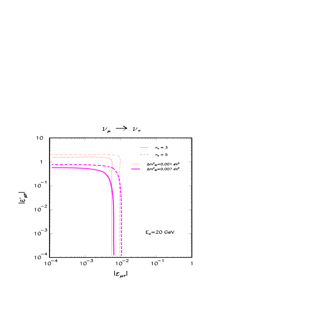
FIG. 3.: Region in the $\epsilon^{\prime}_{\mu\tau}\times\epsilon_{\mu\tau}$ plane that can be probed by a neutrino factory considering $E_{\mu}=20$ GeV, $L=732$ km, $2\times 10^{20}$ muon decays, a 10 kton detector after 5 years of data taking. The regions that were determined by demanding a $n_{\sigma}=3,5$ separation, are the ones to the right of each line. The value of the other oscillation parameters used in this plot are : $\Delta m^{2}_{21}=3.3\times 10^{-5}$ eV², $\sin^{2}2\theta_{23}=0.97$, $\sin^{2}2\theta_{12}=0.78$, $\sin^{2}2\theta_{13}=0.02$ and $\delta=0$. Here $\epsilon_{\mu\tau},\epsilon_{\mu\tau}^{\prime}>0$.

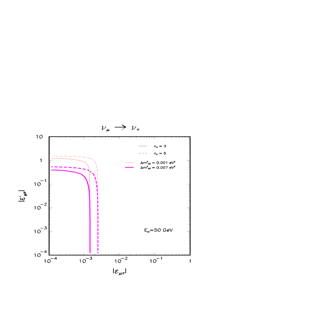
FIG. 4.: Same as Fig. 3 but for $E_{\mu}=50$ GeV.

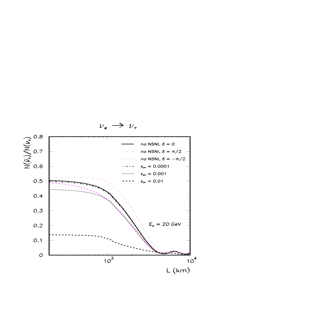
FIG. 5.: Same as Fig. 1 but for the mode $\nu_{e}\rightarrow\nu_{\tau}$/$\bar{\nu}_{e}\rightarrow\bar{\nu}_{\tau}$, we also show the standard case for $\delta=\pi/2,-\pi/2$.

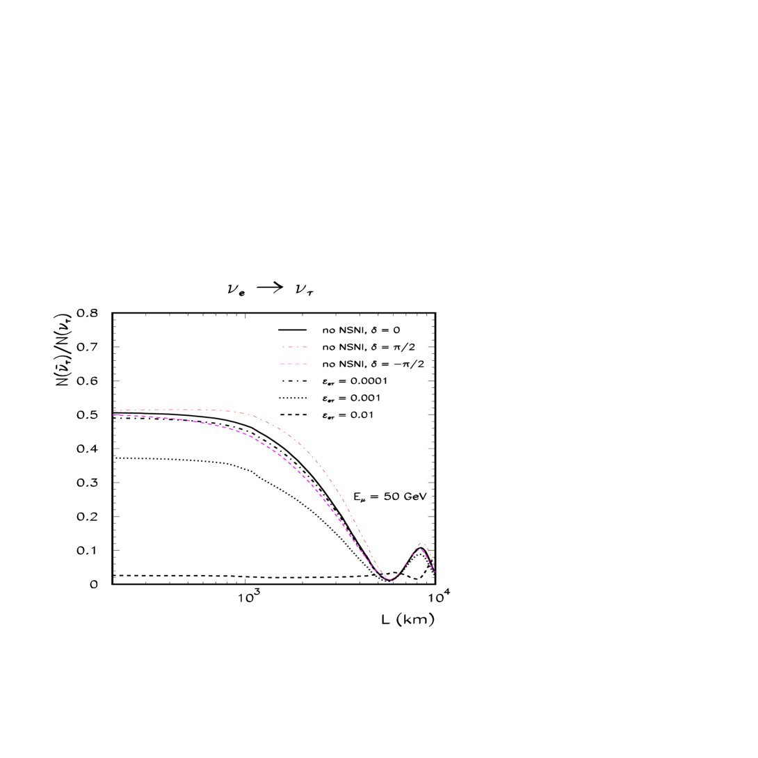
FIG. 6.: Same as Fig. 5 but for $E_{\mu}$ = 50 GeV.

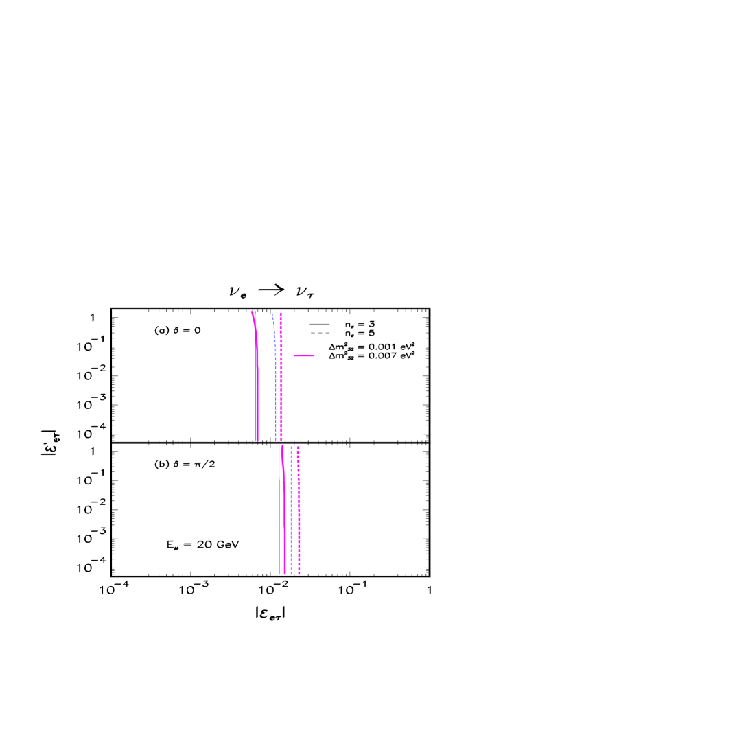
FIG. 7.: Same as Fig. 3 but for the mode $\nu_{e}\rightarrow\nu_{\tau}$/$\bar{\nu}_{e}\rightarrow\bar{\nu}_{\tau}$ and two distinct values of $\delta$. Here $\epsilon_{e\tau},\epsilon_{e\tau}^{\prime}>0$.

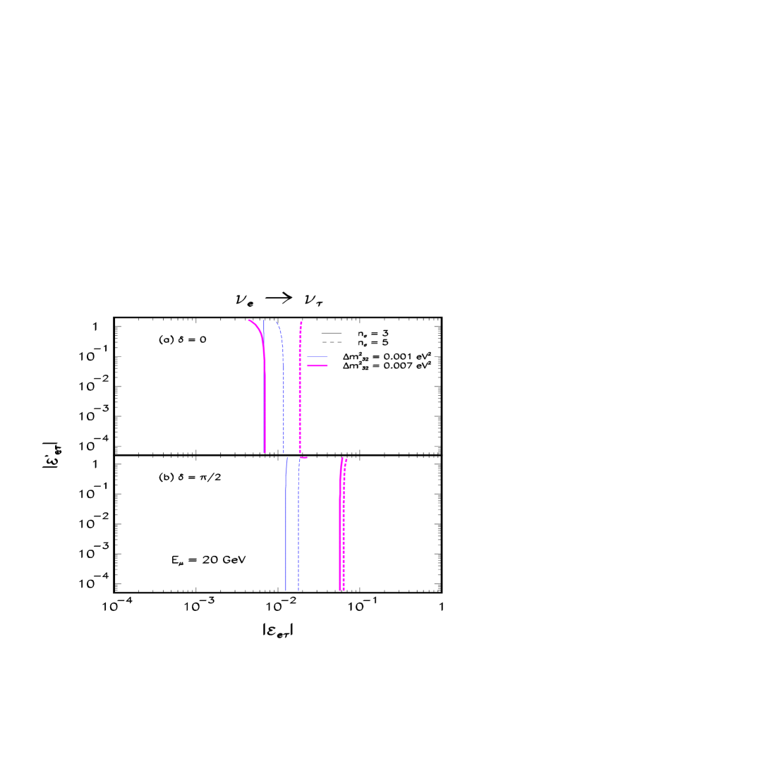
FIG. 8.: Same as Fig. 3 but for the mode $\nu_{e}\rightarrow\nu_{\tau}$/$\bar{\nu}_{e}\rightarrow\bar{\nu}_{\tau}$ and two distinct values of $\delta$. Here $\epsilon_{e\tau},\epsilon_{e\tau}^{\prime}<0$.

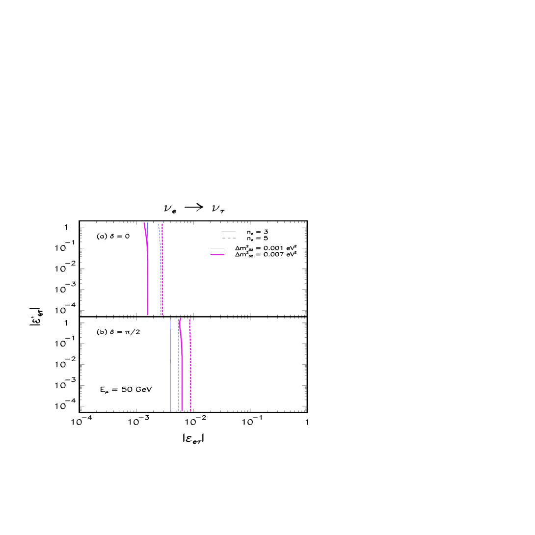
FIG. 9.: Same as Fig. 7 but for $E_{\mu}=50$ GeV.

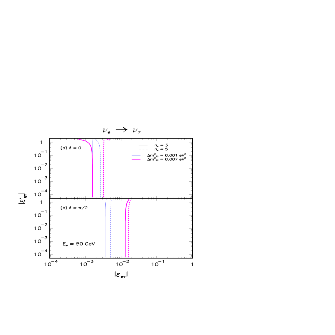
FIG. 10.: Same as Fig. 8 but for $E_{\mu}=50$ GeV.

REFERENCES

• [1] Kamiokande Collaboration, H. S. Hirata et al., Phys. Lett. B 205, 416 (1988); ibid. 280, 146 (1992); Y. Fukuda et al., ibid.  335, 237 (1994); IMB Collaboration, R. Becker-Szendy et al., Phys. Rev. D 46, 3720 (1992); MACRO Collaboration, M. Ambrosio et al., Phys. Lett. B 478, 5 (2000); B. C. Barish, Nucl. Phys. B (Proc. Suppl.) 91, 141 (2001); Soudan-2 Collaboration, W. W. M. Allison et al., Phys. Lett. B 391, 491 (1997); Phys. Lett. B 449, 137 (1999); W. A. Mann, Nucl. Phys. B (Proc. Suppl.) 91, 134 (2001); The Super-Kamiokande Collaboration, Y. Fukuda et al., Phys. Rev. Lett. 81, 1562 (1998); H. Sobel, Nucl. Phys. B (Proc. Suppl.) 91, 127 (2001).
• [2] Homestake Collaboration, K. Lande et al., Astrophys. J. 496, 505 (1998); Kamiokande Collaboration, Y. Fukuta et al., Phys. Rev. Lett. 77, 1683 (1996); GALLEX Collaboration, W. Hampel et al., Phys. Lett. B 447, 127 (1999); GNO Collaboration, M. Altmann et al., Phys. Lett. B 490, 16 (2000); SAGE Collaboration, J. N. Abdurashitov et al., Phys. Rev. C 60, 055801 (1999); V. N. Gavrin, Nucl. Phys. B (Proc. Suppl.) 91, 36 (2001); Y. Suzuki, Nucl. Phys. B (Proc. Suppl.) 91, 29 (2001); Super-Kamiokande Collaboration, S. Fukuda et al., hep-ex/0103032.
• [3] LSND Collaboration, C. Athanassopoulos et al., Phys. Rev. Lett. 77, 3082 (1996); ibid. 81, 1774 (1998); G. B. Mills, Nucl. Phys. B (Proc. Suppl.) 91, 198 (2001); A. Aguilar et al., hep-ex/0104049.
• [4] B. Pontecorvo, Sov. Phys. JETP 26, 984 (1968) [Zh. Eksp. Teor. Fiz. 53, 1717 (1968)].
• [5] Z. Maki, M. Nakagawa, and S. Sakata, Prog. Theor. Phys. 28, 870 (1962).
• [6] D. E. Groom et al., Eur. Phys. J. C, 15, 1 (2000).
• [7] L3 Collaboration, M. Acciarri et al., Phys. Lett. B 431, 199 (1998); DELPHI Collaboration, P. Abreu et al., Z. Phys. C 74, 577 (1997); OPAL Collaboration, R. Akers et al., Z. Phys. C 65, 577 (1995); ALEPH Collaboration, D. Buskulic et al., Phys. Lett. B 313, 520 (1993).
• [8] DONUT Collaboration, K. Kodama et al., Phys. Lett. B 504, 218 (2001).
• [9] S. Fukuda et al., Phys. Rev. Lett. 85, 3999 (2000).
• [10] See for instance: M. C. Gonzalez-Garcia et al., Phys. Rev. D 58, 033004 (1998); M. C. Gonzalez-Garcia, H. Nunokawa, O. L. G. Peres, and J. W. F. Valle, Nucl. Phys. B 543, 3 (1999); N. Fornengo, M. C. Gonzalez-Garcia, and J. W. F. Valle, Nucl. Phys. B 580, 58 (2000).
• [11] O. Yasuda, New Era in Neutrino Physics, ed. by H. Minakata and O. Yasuda, Universal Academic Press, Tokyo, 1999, p.165; Phys. Rev. D 58, 091301 (1998); Acta. Phys. Polon. B 30, 3089 (1999); O. L. Peres and A. Y. Smirnov, Phys. Lett. B 456, 204 (1999); G. L. Fogli, E. Lisi, A. Marrone, and G. Scioscia, Phys. Rev. D 59, 033001 (1999); Nucl. Instrum. Meth. A 451, 10 (2000).
• [12] CHOOZ Collaboration, M. Apollonio et al., Phys. Lett. B 420, 397 (1998); ibid. 466, 415 (1999).
• [13] S. P. Mikheyev and A. Yu. Smirnov, Sov. J. Nucl. Phys. 42, 913 (1985); Nuovo Cimento C9, 17 (1986); L. Wolfenstein, Phys. Rev. D 17, 2369 (1978).
• [14] See for e.g. , M. C. Gonzalez-Garcia, P. C. de Holanda, C. Peña-Garay, and J. W. F. Valle, Nucl. Phys. B 573, 3 (2000); J. N. Bahcall, P. I. Krastev and A. Y. Smirnov, JHEP 0105, 015 (2001) and references there in.
• [15] See for e.g. , G. L. Fogli, E. Lisi, D. Montanino and A. Palazzo, Phys. Rev. D 62, 113004 (2000); A. M. Gago, H. Nunokawa and, R. Zukanovich Funchal, Phys. Rev. D 63, 013005 (2001) and references there in.
• [16] V. Barger, J. G. Learned, S. Pakvasa, and T. J. Weiler, Phys. Rev. Lett. 82, 2640 (1999); V. Barger, J. G. Learned, P. Lipari, M. Lusignoli, S. Pakvasa, and T. J. Weiler, Phys. Lett. B 462, 109 (1999).
• [17] M. C. Gonzalez-Garcia, M. M. Guzzo, P. I. Krastev, H. Nunokawa, O. L. G. Peres, V. Pleitez, J. W. F. Valle, and R. Zukanovich Funchal, Phys. Rev. Lett. 82, 3202 (1999).
• [18] E. Lisi, A. Marrone, and D. Montanino, Phys. Rev. Lett. 85, 1166 (2000).
• [19] P. Lipari and M. Lusignoli, Phys. Rev. D 60, 013003 (1999); N. Fornengo, M. C. Gonzalez-Garcia and J. W. Valle, JHEP 0007, 006 (2000); M. M. Guzzo, H. Nunokawa, O. L. Peres and R. Zukanovich Funchal, Nucl. Phys. Proc. Suppl. 87 (2000) 201.
• [20] K2K Collaboration, S. H. Ahn, et al., hep-ex/0103001.
• [21] See for e.g., M. M. Guzzo and H. Nunokawa, Astropart. Phys. 12, 87 (1999) and references there in.
• [22] See for e.g. S. Bergmann, M. M. Guzzo, P. C. Holanda, P. I. Krastev, and H. Nunokawa, Phys. Rev. D 62, 073001 (2000); M. M. Guzzo, H. Nunokawa, P. C. de Holanda, and O. L. G. Peres, hep-ph/0012089 and references there in.
• [23] See for e.g. A. M. Gago, H. Nunokawa and, R. Zukanovich Funchal, Phys. Rev. Lett. 84, 4035 (2000); Nucl. Phys. B (Proc. Suppl.) 100, 68 (2001) and references there in .
• [24] L. Wolfenstein, in Ref. [13]; ibid. D 20, 2634 (1979).
• [25] M. M. Guzzo, A. Masiero and S. T. Petcov, Phys. Lett. B 260, 154 (1991).
• [26] E. Roulet, Phys. Rev. D 44, 935 (1991).
• [27] J. Schechter and J. W. F. Valle, Phys. Rev. D 22 2227 (1980).
• [28] A. Zee, Phys. Lett. 93B, 389 (1980); K. S. Babu, Phys. Lett. B 203, 132 (1988); for a review see J. W. F. Valle, Prog. Part. Nucl. Phys. 26, 91 (1991).
• [29] F. Zwirner, Phys. Lett. 132B, 103 (1983); J. Ellis et al., Phys. Lett. 150B, 142 (1985); G. G. Ross and J. W. F. Valle, ibid. 151B, 375 (1985).
• [30] H. Nunokawa, hep-ph/0009092.
• [31] See for e.g. , S. Geer, Phys. Rev. D57, 6989 (1998); ibid., Phys. Rev. D59, 039903 (1999); A. De Rujula, M. B. Gavela, and P. Hernandez, Nucl. Phys. B 547 21 (1999). V. Barger, S. Geer, and K. Whisnant, Phys. Rev. D61, 053004 (2000).
• [32] M. Freund, M. Lindner, S. T. Petcov, and A. Romanino, Nucl. Phys. B 578, 27 (2000).
• [33] V. Barger, S. Geer, R. Raja, and K. Whisnant, Phys. Lett. B 485,379 (2000).
• [34] A. Romanino, Nucl. Phys. B 574, 675 (2000).
• [35] A. M. Gago, V. Pleitez, and R. Zukanovich Funchal, Phys. Rev. D 61, 016004 (2000).
• [36] V. Barger, S. Pakvasa, T. J. Weiler, and K. Whisnant, Phys. Rev. Lett. 85, 5055 (2000).
• [37] A. M. Gago, E. M. Santos, W. J. C. Teves, and R. Zukanovich Funchal, Phys. Rev. D 63, 113013 (2001).
• [38] A. Datta, Phys. Lett. B 504, 247 (2001).
• [39] A. Datta, R. Gandhi, and B. Mukhopadhyaya, hep-ph/0011375.
• [40] S. Bergmann and Y. Grossman, Phys. Rev. D59, 093005 (1999); S. Bergmann, Y. Grossman, and D. M. Pierce, Phys. Rev. D 61, 053005 (2000).
• [41] R. Gandhi et al., Astropart. Phys. 5, 81 (1996).
• [42] We have used the fact that at high energies the cross sections scale as : $\sigma_{\nu_{\tau}}(E)=0.67\times 10^{-38}E$ cm2/GeV and $\sigma_{\bar{\nu}_{\tau}}(E)=0.34\times 10^{-38}E$ cm2/GeV.
• [43] C. Albright et al., hep-ex/0008064.
• [44] For discussions on fake CP violation due to matter effetcs, see for e.g. J. Arafune and J. Sato, Phys. Rev. D 55, 1653 (1997); J. Arafune, M. Koike, and J. Sato, Phys. Rev. D 56, 3093 (1997); Erratum ibid., D 60, 119905 (1999); H. Minakata and H. Nunokawa, Phys. Lett. B 413, 369 (1997); Phys. Rev. D 57, 4403 (1998); Phys. Lett. B 495, 369 (2000); M. Tanimoto, Phys. Rev. D 55, 322 (1997); Prog. Theor. Phys. 97, 901 (1997); S. M. Bilenky, C. Giunti, and W. Grimus, Phys. Rev. D 58, 033001 (1998); O. Yasuda, Acta. Phys. Polon. B 30 (1999) 3089; K. Dick, M. Freund, M. Lindner, and A. Romanino, Nucl. Phys. B 562, 29 (1999); T. Ota and J. Sato, Phys. Rev. D 63, 093004 (2001).
• [45] M. C. Gonzalez-Garcia, M. Maltoni, C. Peña-Garay, and J. W. F. Valle, Phys. Rev. D 63, 033005 (2001).
• [46] M. C. Gonzalez-Garcia, Y. Grossman, A. Gusso, and Y. Nir, hep-ph/0105159.