hep-ph/0105160
TUM-HEP-415/01
Alberta Thy 10-01
IFT-15/2001


Two–Loop Matrix Element of the Current–Current Operator in the Decay $B\to X_{s}\gamma$

Abstract

We evaluate the important two–loop matrix element $\langle s\gamma|Q_{2}|b\rangle$ of the operator $\left(\bar{c}\gamma^{\mu}P_{L}b\right)\left(\bar{s}\gamma_{\mu}P_{L}b\right)$ contributing to the inclusive radiative decay $B\rightarrow X_{s}\gamma$. The calculation is performed in the NDR scheme, by means of asymptotic expansions method. The result is given as a series in $z\equiv m_{c}^{2}/m_{b}^{2}$ up to ${\cal O}(z^{6})$. We confirm the result of Greub, Hurth and Wyler obtained by a different method up to ${\cal O}(z^{3})$. Higher–order terms are found to be numerically insignificant.

xxx

1 Introduction

The radiative decay $B\to X_{s}\gamma$ plays an important role in the present tests of the Standard Model (SM) and of its extensions [1]. In particular, in the supersymmetric extensions of the SM, the best bounds on several new parameters come from the data on $B\to X_{s}\gamma$ [2].

The short distance QCD effects are very important for this decay. They are known to enhance the branching ratio ${\rm Br}(B\to X_{s}\gamma)$ by roughly a factor of three, as first pointed out in [3, 4]. Since these first analyses, a lot of progress has been made in calculating these important QCD effects in the renormalization group improved perturbation theory, beginning with the work in [5, 6]. Let us briefly summarize this progress.

A peculiar feature of the renormalization group analysis in $B\to X_{s}\gamma$ is that the mixing under infinite renormalization between the four-fermion operators $(Q_{1},\ldots,Q_{6})$ and the magnetic penguin operators $(Q_{7\gamma},Q_{8G})$, which govern this decay, vanishes at the one-loop level. Consequently, in order to calculate the coefficients $C_{7\gamma}(\mu_{b})$ and $C_{8G}(\mu_{b})$ at $\mu_{b}={\cal O}(m_{b})$ in the leading logarithmic approximation, two-loop calculations of ${\cal{O}}(eg^{2}_{s})$ and ${\cal{O}}(g^{3}_{s})$ are necessary. Such calculations were completed in [7, 8] and confirmed in [9, 10, 11]. Earlier analyses contained either additional approximations or mistakes.

It turns out that the leading order expression for the branching ratio ${\rm Br}(B\to X_{s}\gamma)$ suffers from sizable renormalization scale uncertainties [12, 13] implying that a complete NLO analysis including also dominant higher order electroweak effects to this decay is mandatory. By 1998, the main ingredients of such an analysis had been calculated. It was a joint effort of many groups:

• The ${\cal O}(\alpha_{s})$ corrections to $C_{7\gamma}(\mu_{W})$ and $C_{8G}(\mu_{W})$ were first calculated in [14] and subsequently confirmed by several groups [15]–[18].

• The two-loop mixing involving the four fermion operators $Q_{1},\ldots,Q_{6}$ and the two-loop mixing in the sector $(Q_{7\gamma},Q_{8G})$ was calculated in [19]–[24] and [25], respectively. The very difficult three-loop mixing between the set $(Q_{1},\ldots,Q_{6})$ and the operators $(Q_{7\gamma},Q_{8G})$ was calculated in [11].

• Leading order matrix elements $\langle s\gamma\;{\rm gluon}|Q_{i}|b\rangle$ were calculated in [26, 27], and the challenging two-loop calculation of $\langle s\gamma|Q_{2}|b\rangle$ was presented in [28].

• Higher order electroweak corrections were incorporated with increasing level of sophistication in [29]–[33].

In addition, non-perturbative corrections were calculated in [34]–[39]. The most recent analysis of $B\to X_{s}\gamma$ incorporating all these calculations can be found in [40].

Now, among the perturbative ingredients listed above, three have been calculated only by one group. These are

• The two-loop mixing in the sector $(Q_{7\gamma},Q_{8G})$ [25].

• The three-loop mixing between the set $(Q_{1},\ldots,Q_{6})$ and the operators $(Q_{7\gamma},Q_{8G})$ [11].

• The two-loop matrix element $\langle s\gamma|Q_{2}|b\rangle$ [28].

Moreover,

• The two-loop matrix elements of the QCD penguin operators $\langle s\gamma|Q_{i}|b\rangle$ with $i=3,\ldots,6$ have not yet been calculated.

It should be emphasized that all these four ingredients enter not only the analysis of $B\to X_{s}\gamma$ in the SM but are also necessary ingredients of any analysis of this decay in the extensions of this model. It is therefore desirable to check the first three calculations and to perform the last one.

In the present paper, we will make the first step in this direction by calculating the two-loop matrix element $\langle s\gamma|Q_{2}|b\rangle$ using the method of asymptotic expansions. This matrix element turned out [28, 40] to be the most important ingredient of the NLO–analysis for Br$(B\rightarrow X_{s}\gamma)$ enhancing this branching ratio by roughly $20\%$. In [28], the matrix element $\langle s\gamma|Q_{2}|b\rangle$ was found by applying the Mellin–Barnes representation to certain internal propagators, and the result was presented as an expansion in $z=m_{c}^{2}/m_{b}^{2}$ up to and including terms ${\cal O}(z^{3})$. In order to be sure about the convergence of this expansion, we will include also the terms ${\cal O}(z^{4})$, ${\cal O}(z^{5})$ and ${\cal O}(z^{6})$.

2 Two-Loop Contribution to $\langle s\gamma|Q_{2}|b\rangle$.

2.1 Preface

The effective Hamiltonian for the process $b\rightarrow s\gamma$ is given by

$$H_{\rm eff}(b\rightarrow s\gamma)=-\frac{4G_{F}}{\sqrt{2}}V_{tb}V_{ts}^{*}\sum_{i=1}^{8}C_{i}(\mu)Q_{i}.$$ (2.1)

Here $G_{F}$ is the Fermi constant, $V_{ij}$ are the CKM matrix elements and $C_{i}$ are the Wilson coefficients of the operators $Q_{i}$ evaluated at $\mu={\cal O}(m_{b})$. We have dropped the negligible contributions proportional to $V_{ub}V_{us}^{*}$. The full list of operators in (2.1) can be found in [28]. In the present paper we need only the expressions for two of them. These are

$$Q_{2} = \left(\bar{c}\gamma^{\mu}P_{L}b\right)\left(\bar{s}\gamma_{\mu}P_{L}b\right),$$ (2.2)

$$Q_{7} = \frac{e}{16\pi^{2}}\bar{s}_{\alpha}\sigma^{\mu\nu}(m_{b}(\mu)P_{R}+m_{s}(\mu)P_{L})b_{\alpha}F_{\mu\nu},$$ (2.3)

where $P_{L}=(1-\gamma_{5})/2$, $P_{R}=(1+\gamma_{5})/2$ and $\sigma^{\mu\nu}={i\over 2}[\gamma_{\mu},\gamma_{\nu}]$. As in [28], we will set $m_{s}=0$.

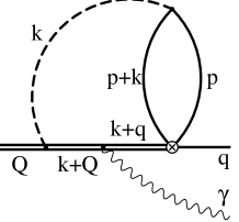
Figure 4: Diagram $M_{2}$.

In this section, we present the details of the calculation of the matrix element $\langle s\gamma|Q_{2}|b\rangle$ in the NDR scheme. This matrix element vanishes at the one-loop level. Therefore, in order to obtain a non-vanishing contribution, one has to calculate two-loop diagrams. They are shown in Figs. 1, 4, 5, and 6, where the wavy and dashed lines represent the photon and gluon, respectively. Following [28], we have divided the contributing diagrams into four sets:

• In sets 1 and 2, the photon is emitted from an internal s-quark (set1) or an internal b-quark (set 2), which also exchanges a gluon with the charm quark.

• Sets 3 and 4 are obtained from sets 1 and 2, respectively, by emitting this time the photon from the charm quark propagator.

• Thanks to QED gauge invariance, it is not necessary to consider diagrams with a real photon emission from external quark lines.

It is convenient to write the regularized contributions from each set of the diagrams as follows:

$$M_{1} = \left\{{1\over 36\epsilon}\left({m_{b}\over\kappa\mu}\right)^{-4\epsilon}+\widetilde{M}_{1}\right\}{\alpha_{s}\over\pi}\,C_{F}Q_{d}\,\langle s\gamma|Q_{7}|b\rangle_{\rm tree},$$ (2.4)

$$M_{2} = \left\{-{5\over 36\epsilon}\left({m_{b}\over\kappa\mu}\right)^{-4\epsilon}+\widetilde{M}_{2}\right\}{\alpha_{s}\over\pi}\,C_{F}Q_{d}\,\langle s\gamma|Q_{7}|b\rangle_{\rm tree},$$ (2.5)

$$M_{3} = \left\{-{1\over 8\epsilon}\left({m_{b}\over\kappa\mu}\right)^{-4\epsilon}+\widetilde{M}_{3}\right\}{\alpha_{s}\over\pi}\,C_{F}Q_{u}\,\langle s\gamma|Q_{7}|b\rangle_{\rm tree},$$ (2.6)

$$M_{4} = \left\{-{1\over 4\epsilon}\left({m_{b}\over\kappa\mu}\right)^{-4\epsilon}+\widetilde{M}_{4}\right\}{\alpha_{s}\over\pi}\,C_{F}Q_{u}\,\langle s\gamma|Q_{7}|b\rangle_{\rm tree}.$$ (2.7)

We work in $D=4-2\epsilon$ dimensions, with $\kappa^{2}=4\pi e^{-\gamma_{E}}$, $Q_{u}=\frac{2}{3}$, $Q_{d}=-\frac{1}{3}$, $C_{F}=\frac{4}{3}$ and $\gamma_{E}$ is Euler’s constant. The tree level matrix element of the operator $Q_{7}$ is given by

$$\,\langle s\gamma|Q_{7}|b\rangle_{\rm tree}=m_{b}(\mu_{b}){e\over 8\pi^{2}}\overline{u}(p^{\prime})\epsilon/q/P_{R}u(p).$$ (2.8)

In order to make the two-loop matrix element finite, counterterms have to be added. These counterterms can easily be calculated by using the operator renormalization constants that were needed in the context of the calculation of the leading order anomalous dimension matrix. The complete counterterm is found to be [28]

$$M_{2}^{\rm count}=\left\{{Q_{d}\over 6}\left({m_{b}\over\mu}\right)^{-2\epsilon}+{3Q_{u}\over 8}-{Q_{d}\over 18}\right\}{\kappa^{4\epsilon}\over\epsilon}\;{\alpha_{s}\over\pi}\,C_{F}\,\langle s\gamma|Q_{7}|b\rangle_{\rm tree}.$$ (2.9)

The above expression includes two-loop counterterms as well as contributions from one-loop diagrams with one-loop counterterm insertions.

Adding the contributions from (2.4)–(2.7) and (2.9), we find the two-loop matrix element $\langle s\gamma|Q_{2}|b\rangle$ in the NDR-scheme:

$$\langle s\gamma|Q_{2}|b\rangle=\,\langle s\gamma|Q_{7}|b\rangle_{\rm tree}{\alpha_{s}\over 4\pi}\left({416\over 81}\ln{m_{b}\over\mu}+r_{2}\right),$$ (2.10)

with

$$r_{2}=-{16\over 9}(\widetilde{M}_{1}+\widetilde{M}_{2})+{32\over 9}(\widetilde{M}_{3}+\widetilde{M}_{4}).$$ (2.11)

The rest of this section is devoted to a detailed presentation of the calculation of the contributions $\widetilde{M}_{i}$ using the method of asymptotic expansions. All the momentum integrals are performed in the Euclidean space.

2.2 Diagram $M_{1}$

Of the four sets of diagrams which we have to consider, $M_{1}$ and $M_{2}$ shown in Fig. 1 and 4 are relatively simple. In $M_{1}$, the photon is emitted from a massless $s$-quark propagator, and the two-loop integral factorizes into the $c$-quark loop and the one-loop vertex integral. There are four momentum regions we have to consider. Denoting the momenta in the $c$-quark and vertex loops by $p$ and $k$, we have

1. $k\sim p\sim m_{b}$: the “hard-hard” region;

2. $k\sim m_{b}$ and $p\sim m_{c}$: the “hard-soft” region (which comes in two variants, depending on the routing of $k$ through the $c$-quark loop);

3. a “collinear-soft” region, in which $p\sim m_{c}$ and $k\cdot\gamma\sim m_{b}^{2}$ but $k\cdot q\sim m_{c}^{2}$.

Below, we describe the treatment of those regions in some detail.

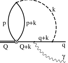
Figure 1: Diagram $M_{1}$. Momentum assignments: $Q$, $q$, and $\gamma$ denote respectively four-momenta of the $b$ and $s$ quarks, and of the photon; $p$ and $k$ are loop momenta. Double lines denote a massive particle (the $b$ quark) and single lines are light particle propagators. The gluon is denoted by a dashed line.

2.2.1 Hard contribution: Taylor expansion in $m_{c}$

Since all scalar products are now large compared with $m_{c}^{2}$, we can expand the $c$-quark propagators in $m_{c}$. This leads to a massless loop integration, which simply modifies the power of the momentum ($k$) in the gluon propagator (see Fig. 2). After this first integration, the integrand has the following form:

$$\int{{\rm d}^{D}k\;\mbox{(scalar products involving $k$)}\over(k^{2})^{a_{1}+\epsilon}(k^{2}+2k\cdot Q+Q^{2})^{a_{2}}(k^{2}+2k\cdot q)^{a_{3}}}.$$ (2.12)

We combine propagators 1 and 3 using the Feynman parameter $x$, and then combine the result ($\cdot(1-y)$) with propagator 2 ($\cdot y$). We shift the variable $k\to K-x(1-y)q-yQ$, and the denominator becomes a power of $k^{2}+y(1-y)(x-1-i0)$. Since $x-1<0$, this diagram has an imaginary part; its sign is determined by assigning a small negative imaginary mass to the massless lines. After the momentum shift, we have additional factors $x^{m}$ and $y^{n}$ in the numerator, and denominator has the power $d+\epsilon$. The result is

$$\left[\exp(-i\pi)\right]^{-2\epsilon}(-1)^{d}{\Gamma(d-2+2\epsilon)\over\Gamma(d+\epsilon)}{B(m+a_{3},a_{1}+2-d-\epsilon)\over B(a_{3},a_{1}+\epsilon)B(a_{2},a_{1}+a_{3}+\epsilon)}$$

$$\times B(n+a_{2}+2-d-2\epsilon,a_{1}+a_{3}+2-d-\epsilon),$$ (2.13)

where $B$ and $\Gamma$ are the standard Euler functions Beta and $\Gamma$.

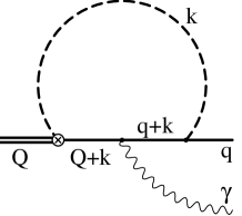
Figure 2: One-loop diagram (the $k$ propagator can have fractional power) corresponding to eq. (2.12).

2.2.2 Hard-soft contributions from $k\sim m_{b}$, $p\sim m_{c}$

This region can be handled as in the “large momentum expansion” [41, 42, 43]. In Fig. 3, we see one of the two configurations to be computed. We first integrate over $p$, and then evaluate the one-loop vertex. An analogous procedure is executed for the other (left) $c$-quark line.

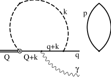
Figure 3: Subgraph corresponding to one of the two hard-soft contributions.

2.2.3 Collinear region

Naively, one might think that we should consider the region $k\sim p\sim m_{c}$, in which $(Q+k)^{2}\simeq Q^{2}$, $(q+k)^{2}\simeq 2k\cdot q$. However, this does not lead to a consistent power counting, since we have to shift the momentum $k$ by an amount proportional to $q$, which is $\sim m_{b}$.

Instead, we have to consider the collinear configurations [44]. We define

$$k\cdot q=Q_{0}k_{-}, k\cdot\gamma=Q_{0}k_{+},\quad k^{2}=k_{+}k_{-}-k_{\perp}^{2},\quad Q^{2}=Q_{0}^{2},\quad k\cdot Q=Q_{0}(k_{+}+k_{-}).$$

The relevant contribution is $k_{+}\sim Q_{0}$, $k_{-}\sim{m_{c}^{2}\over Q_{0}}$. Now $(Q+k)^{2}\simeq Q^{2}+2k\cdot\gamma$, while $(k+q)^{2}=k^{2}+2k\cdot q$ is already homogeneously of order $m_{c}^{2}$ and cannot be expanded. First, we integrate over $p$; for this we combine the two $c$ propagators (we assume here, for generality, that their powers are $a_{1}$ and $a_{2}$) using $x$, shift $p\to P-xk$, and obtain ($m$ and $d$ are exponents arising from the presence of $p$ in the numerator)

$${{\rm polynomial}(p)\over\left[(p+k)^{2}+m_{c}^{2}\right]^{a_{1}}\left[p^{2}+m_{c}^{2}\right]^{a_{2}}} \to {\Gamma(d-2+\epsilon)\over B(a_{1},a_{2})\Gamma(d)}{x^{m+a_{1}+1-d-\epsilon}(1-x)^{a_{2}+1-d-\epsilon}\over(k^{2}+m_{x}^{2})^{d-2+\epsilon}},$$

$$m_{x}^{2} \equiv {m_{c}^{2}\over x(1-x)}.$$ (2.15)

For the $k$ integration, the integrand has the form

$$\int{{\rm d}^{D}k\;\;{\rm polynomial}(k)\over(k^{2})^{a_{3}}(k^{2}+m_{x}^{2})^{d-2+\epsilon}(k^{2}+2k\cdot q)^{a_{4}}(Q^{2}+2\gamma\cdot k)^{a_{5}}}.$$ (2.16)

Now, we combine the first two propagators multiplying them by $1-z$ and $z$, respectively. We multiply the result by $y$ and combine it with the “$a_{4}$” propagator multiplied by $1-y$. Finally, we use the parameter $u$ to include the last propagator ($i=a_{3}+a_{4}+d-2+\epsilon$):

$${1\over[k^{2}+yzm_{x}^{2}+2(1-y)k\cdot q]^{i}\;(Q^{2}+2k\cdot\gamma)^{a_{5}}}$$ (2.17)

$$={1\over B(i,a_{5})}\int_{0}^{\infty}{\rm d}u\;{u^{a_{5}-1}\over[k^{2}+yzm_{x}^{2}+2(1-y)k\cdot q+2uk\cdot\gamma+uQ^{2}]^{i+a_{5}}}.$$

Now, we shift $k\to K-(1-y)q-u\gamma$ and, using $q\cdot\gamma=Q^{2}/2$, find that the denominator simplifies to become $[K^{2}+y(zm_{x}^{2}+uQ^{2})]$. Because of the presence of $K$ in the numerator, we generate additional powers of Feynman parameters. After integrating over $K$, we integrate over $u$,

$$\int_{0}^{\infty}{\rm d}u\;{u^{n-1}\over(zm^{2}+uQ^{2})^{m}}={B(n,m-n)\over(Q^{2})^{n}(zm^{2})^{m-n}}.$$ (2.18)

We see that the dependence on $Q$ separates (so the integral really depends only on a single scale). Also, only $m_{c}$ appears in fractional power, so that there is no imaginary part in this integral, even though $Q^{2}<0$ (after the Wick rotation).

2.3 $M_{2}$

In this diagram, we have again four momentum regions, of which the first three are similar to those discussed for $M_{1}$. The fourth one is different: it is a “soft-soft” contribution, with $k\sim p\sim m_{c}$.

For the hard-hard contribution, we first integrate over $p$, just like in $M_{1}$. After that, the integrand takes on the following form:

$$\int{{\rm d}^{D}k\;\mbox{(scalar products involving $k$)}\over(k^{2})^{a_{1}+\epsilon}(k^{2}+2k\cdot Q)^{a_{2}}(k^{2}+2k\cdot q-Q^{2})^{a_{3}}}.$$ (2.19)

We combine propagators 2 and 3 using a Feynman parameter $x$, and then combine the result ($\cdot y$) with the propagator 1 ($\cdot(1-y)$). We shift the variable $k\to K-y((1-x)Q+xq)$, and the denominator becomes a power of $k^{2}+y[y+x(1-y)]$. After shifting the momentum and simplifying the numerator, additional factors $x^{m}$ and $y^{n}$ appear in the numerator, and the denominator has the power $d+2\epsilon$. After the $k$ integration, we find that the $x$ and $y$ integrations do not separate, and we first integrate over $x$ using eq. (2.30), to be discussed below. The remaining $y$ integration is a Beta function.

The hard-soft contributions are similar to those in $M_{1}$ and lead to rather trivial products of one-loop integrals.

On the other hand, the soft-soft contribution is less standard. We have $k\sim m_{c}$ and the two $b$-quark propagators can be expanded. In the lowest order we have

$${1\over k^{2}+2k\cdot Q} \to {1\over 2k\cdot Q},$$

$${1\over k^{2}+2k\cdot q-Q^{2}} \to -{1\over Q^{2}}.$$ (2.20)

Since the second propagator becomes independent of $k$, the whole two-loop diagram becomes equivalent to a simpler, two-point function. The resulting integrals are similar, but not the same, as those considered in the eikonal expansion study [45]. Details of their evaluation have been recently described in a completely different context of bound-state calculations [46]. In that work, exactly such type of integrals appeared when energies of bound-states consisting of two particles with very different masses were expressed as expansions in the ratio of those masses.

2.4 $M_{3}$

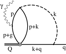
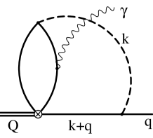
(a)	(b)

Figure 5: Diagrams contributing to $M_{3}$, with photon emission from two $c$-quark lines.

This diagram, shown in Fig. 5, is the first of the two non-trivial two-loop vertex diagrams we have to consider. There are now five momentum regions to be considered:

1. Hard-hard, $k\sim p\sim m_{b}$, similar to those of $M_{1,2}$.

2. Hard-soft, $k\sim m_{b}$, $p\sim m_{c}$, which now enters only once, when hard momentum flows through the same $c$-quark line from which the photon is emitted.

3. Collinear-collinear, with $k$ and $p$ having their only large components (${\cal O}\left(m_{b}\right)$) aligned with the $s$-quark momentum $q$ (and with $k^{2}\sim p^{2}\sim m_{c}^{2}$).

4. Collinear-collinear, but with the alignment with the photon momentum $\gamma$.

5. Hard-collinear, where $k\sim m_{b}$ and $p$ is aligned parallel with $\gamma$.

The first two regions are treated in an analogous manner as was described for $M_{1,2}$. In the hard-hard contribution, after expansion in $m_{c}$, the integrand is symmetrical (apart from different powers of propagators) under replacement $p\leftrightarrow k$, $\gamma\leftrightarrow q$. Hence, we can first integrate over $k$, and then over $p$. Both integrations are very similar to those in $M_{1,2}$. In the second region, we use the “large momentum expansion” mentioned in Section 2.2.2.

The collinear-collinear regions require more attention [47]. After expansion of the integrands in the available small quantities, it turns out that the integrals over Feynman parameters have singularities (like $\int_{0}{\rm d}x/x$) which are not regularized by our dimensional regulator. It is necessary to introduce additional, analytical regularization on the heavy quark line. Similar phenomena have been observed before (see e.g. [47] and references therein). Nevertheless, all integrals over the Feynman parameters can be evaluated analytically without particular difficulties. Dependence on the analytical regulator cancels in the sum of the two doubly-collinear contributions.

2.5 $M_{4}$

The most complicated diagram is $M_{4}$, depicted in Fig. 6. There are six momentum regions:

1. Hard-hard.

2. Hard-soft.

3. Collinear-collinear with alignment along $\gamma$. There is no contribution with alignment along $q$ here, because of the different structure of the internal quark propagator, which now contains the large $b$-quark mass.

4. Hard-collinear, as in $M_{3}$.

5. Ultrasoft-collinear [47], with $k\sim m_{c}^{2}/m_{b}$ and $p$ aligned with $\gamma$.

6. Soft-soft.

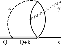
(a)	(b)

Figure 6: Diagram $M_{4}$

We give a more detailed description of the hard-hard contribution, because the integrals resulting here are rather complicated. First, we consider the scalar integral with all propagators in the first power,

$$J_{3}=\int{{\rm d}^{D}k\over k^{2}(k^{2}+2Q\cdot k)}\int{{\rm d}^{D}p\over p^{2}(p-k)^{2}(p+\gamma)^{2}}.$$ (2.21)

We first evaluate the massless ($c$ quark) loop (integrals over all Feynman parameters run from 0 to 1):

$$\int{{\rm d}^{D}p\over p^{2}(p-k)^{2}(p+\gamma)^{2}} = \int{{\rm d}^{D}p\over p^{2}(p^{2}-2p\cdot k+k^{2})(p^{2}+2p\cdot\gamma)}$$ (2.22)

$$= \int 2(1-y){\rm d}y\;{\rm d}x\;\int{{\rm d}^{D}p\over[p^{2}-2yp\cdot k+2x(1-y)p\cdot\gamma+yk^{2}]^{3}}$$

$$= \Gamma(1+\epsilon)\,\pi^{2-\epsilon}\int{y^{-1-\epsilon}(1-y)^{-\epsilon}{\rm d}y\;{\rm d}x\over(k^{2}+2xk\cdot\gamma)^{1+\epsilon}}$$

$$= \Gamma(1+\epsilon)B(-\epsilon,1-\epsilon)\,\pi^{2-\epsilon}\int{{\rm d}x\over(k^{2}+2xk\cdot\gamma)^{1+\epsilon}}.$$

In the process of the integration, we made a shift $p\to p+yk-x(1-y)\gamma$. Next, we integrate over $k$:

$$\int{\rm d}x\int{{\rm d}^{D}k\over k^{2}(k^{2}+2Q\cdot k)(k^{2}+2xk\cdot\gamma)^{1+\epsilon}}$$ (2.23)

$$= (1+\epsilon)\int{\rm d}x\;{\rm d}u\;(1-u)^{\epsilon}\int{{\rm d}^{D}k\over k^{2}[k^{2}+2uk\cdot Q+2(1-u)xk\cdot\gamma]^{2+\epsilon}}$$

$$= (2+\epsilon)(1+\epsilon)\int{\rm d}z\;z^{1+\epsilon}{\rm d}x\;{\rm d}u\;(1-u)^{\epsilon}\int{{\rm d}^{D}k\over[k^{2}+z^{2}u^{2}+z^{2}u(1-u)x]^{3+\epsilon}}$$

$$= {\Gamma(1+2\epsilon)\over\Gamma(1+\epsilon)}\,\pi^{2-\epsilon}\int{\rm d}z\;{\rm d}x\;{\rm d}u\;{z^{-1-3\epsilon}u^{-1-2\epsilon}(1-u)^{\epsilon}\over[u+(1-u)x]^{1+2\epsilon}}$$

$$= {\Gamma(1+2\epsilon)\over 6\epsilon^{2}\Gamma(1+\epsilon)}\,\pi^{2-\epsilon}\int{\rm d}u\;u^{-1-2\epsilon}(1-u)^{-1+\epsilon}(1-u^{-2\epsilon})$$

$$= {\Gamma(1+2\epsilon)\over 6\epsilon^{2}\Gamma(1+\epsilon)}\,\pi^{2-\epsilon}\left[B(-2\epsilon,\epsilon)-B(-4\epsilon,\epsilon)\right].$$

We made a shift $k\to k-zuQ-z(1-u)x\gamma$ and used $Q^{2}=2Q\cdot\gamma=-1$. Multiplying the result (2.23) with the coefficient $\Gamma(1+\epsilon)B(-\epsilon,1-\epsilon)$ from (2.22) we find

$$J_{3} = {\Gamma(1+2\epsilon)\over 6\epsilon^{2}}B(-\epsilon,1-\epsilon)\left[B(-2\epsilon,\epsilon)-B(-4\epsilon,\epsilon)\right]$$ (2.24)

$$= \Gamma(1+\epsilon)^{2}\left({1\over 24\epsilon^{4}}+{\pi^{2}\over 18\epsilon^{2}}+{7\over 6\epsilon}\zeta_{3}+{29\pi^{4}\over 360}\right)+{\cal O}\left(\epsilon\right).$$

Now we consider the general case, in which momenta $p$ and $k$ can be present in the numerator,

$$\int{{\rm d}^{D}k\;{\rm d}^{D}p\;\mbox{(scalar products involving $k$ and $p$)}\over{(k^{2})}^{a_{1}}{(k^{2}+2k\cdot Q)}^{a_{2}}{(p-k)}^{2a_{3}}{(p^{2})}^{a_{4}}{(p^{2}+2p\cdot\gamma)}^{a_{5}}}.$$ (2.25)

We first combine the propagators 5 ($\cdot x$) and 4 ($\cdot(1-x)$), and then the result ($\cdot(1-y)$) with 3 ($\cdot y$). We shift the integration momentum $p=K-x(1-y)\gamma+yk$ and average over $K$. This again results in extra powers $y^{n}$ and $x^{m}$, while canceling powers of $K^{2}$ changes the power of the denominator. After the integration over $K$, the denominator becomes $[y(1-y)(k^{2}+2xk\cdot\gamma)]^{d-2+\epsilon}$. We see that the dependence on $y$ factorizes and we can integrate over this variable. As a result, we find an expression of the form

$${\Gamma(a_{3}+a_{4}+a_{5})\Gamma(d-2+\epsilon)B(n+a_{3}-d+2-\epsilon,a_{4}+a_{5}-d+2-\epsilon)\over\Gamma(a_{3})\Gamma(a_{4})\Gamma(a_{5})\Gamma(d)}$$ (2.26)

$$\times\int{\rm d}x\;x^{a_{5}+m-1}(1-x)^{a_{4}-1}\rule{85.35826pt}{0.0pt}$$ (2.27)

$$\times\int{{\rm d}^{D}k\;\mbox{(scalar products involving $k$)}\over{(k^{2})}^{a_{1}}{(k^{2}+2k\cdot Q)}^{a_{2}}{(k^{2}+2xk\cdot\gamma)}^{d-2+\epsilon}}.\rule{5.69054pt}{0.0pt}$$ (2.28)

We now repeat a similar procedure with the variable $p$. We combine the propagator 2 ($\cdot u$) with $(k^{2}+2xk\cdot\gamma)$ ($\cdot(1-u)$), and then the result ($\cdot z$) with the propagator 1 ($\cdot(1-z)$). We change the momentum variable $k=K-zuQ-zx(1-u)\gamma$, average over $K$ and simplify powers of $K^{2}$ (as a result, the power of the denominator changes from $a_{1}+a_{2}+d-2$ to some $d_{1}$, and we also get extra powers $z^{e}$ and $u^{w}$). After integrating over $K$ we get (including the factors (2.26,2.27))

$${\Gamma(a_{3}+a_{4}+a_{5})\Gamma(d-2+\epsilon)B(n+a_{3}-d+2-\epsilon,a_{4}+a_{5}-d+2-\epsilon)\over\Gamma(a_{3})\Gamma(a_{4})\Gamma(a_{5})\Gamma(d)}$$ (2.29)

$$\times {\Gamma(d_{1}-2+2\epsilon)\Gamma(a_{1}+a_{2}+d-2+\epsilon)B(a_{1},a_{2}+d+2+e-2d_{1}-3\epsilon)\over\Gamma(d_{1}+\epsilon)\Gamma(a_{1})\Gamma(a_{2})\Gamma(d-2+\epsilon)}$$

$$\times \int{\rm d}x\;{\rm d}u\;x^{a_{5}+m-1}(1-x)^{a_{4}-1}u^{w+a_{2}+1-d_{1}-2\epsilon}(1-u)^{d-3+\epsilon}\left[u+x(1-u)\right]^{2-d_{1}-2\epsilon}.\rule{28.45274pt}{0.0pt}$$

First we integrate over $x$, using

$$\int_{0}^{1}{\rm d}x\;x^{n}\left[u+x(1-u)\right]^{\mu}={u^{\mu+n+1}\over(1-u)^{n+1}}\sum_{j=0}^{n}(-1)^{j}{n\choose j}{u^{j-1-n-\mu}-1\over\mu+n+1-j}.$$ (2.30)

This integration is possible because the powers of $x$ and $(1-x)$ in (2.27) are non-negative integer. The $u$ integration gives a simple Beta function.

The techniques described above are sufficient to compute all the remaining contributions. Again, the dimensional regularization alone is insufficient to evaluate the doubly-collinear contribution. We introduce an analytical regulator on the heavy quark mass. The resulting singularities vanish when we add the soft-soft contribution.

2.6 Results

The final results for $\widetilde{M}_{i}$ are listed below, with $z=m_{c}^{2}/m_{b}^{2}$ and $L=\ln z$.

$$\widetilde{M}_{1} = {37\over 216}+\left(-{5\over 2}-L\right)z+\left(-{5\over 2}+\pi^{2}+L-L^{2}\right)z^{2}$$ (2.31)

$$+\left(-{17\over 27}-{2\over 3}\pi^{2}-{10\over 9}L+{2\over 3}L^{2}\right)z^{3}$$

$$+\left(-{11\over 12}+L\right)z^{4}+\left(-{1\over 30}+{2\over 3}L\right)z^{5}+\left({67\over 270}+{7\over 9}L\right)z^{6}$$

$$+i\pi\left[{1\over 18}-z+(1-2L)z^{2}+\left(-{10\over 9}+{4\over 3}L\right)z^{3}+z^{4}+{2\over 3}z^{5}+{7\over 9}z^{6}\right],$$

$$\widetilde{M}_{2} = {13\over 216}+\left(-{1\over 2}+{1\over 6}\pi^{2}\right)z-{2\over 3}\pi^{2}z^{{3\over 2}}+\left(3-3L+{1\over 2}L^{2}\right)z^{2}$$ (2.32)

$$+\left(-{157\over 108}+{5\over 9}\pi^{2}+{1\over 18}L+{4\over 3}L^{2}\right)z^{3}+\left(-{4679\over 900}+{2\over 3}\pi^{2}+{107\over 30}L+2L^{2}\right)z^{4}$$

$$+\left(-{26185\over 2352}+{5\over 3}\pi^{2}+{277\over 28}L+5L^{2}\right)z^{5}$$

$$+\left(-{2831737\over 97200}+{14\over 3}\pi^{2}+{16177\over 540}L+14L^{2}\right)z^{6},$$

$$\widetilde{M}_{3} = -{15\over 16}+\left({3\over 2}-{1\over 2}\pi^{2}L-{1\over 4}\pi^{2}-2\zeta_{3}+2L+{1\over 4}L^{2}+{1\over 6}L^{3}\right)z$$ (2.33)

$$+\left({5\over 4}-{1\over 2}\pi^{2}L+{1\over 2}\pi^{2}-2\zeta_{3}+{1\over 2}L-{1\over 2}L^{2}+{1\over 6}L^{3}\right)z^{2}$$

$$+\left(-{17\over 12}+L\right)z^{3}+\left(-{7\over 216}+{5\over 9}L\right)z^{4}$$

$$+\left({1183\over 4320}+{49\over 72}L\right)z^{5}+\left({8783\over 12000}+{231\over 200}L\right)z^{6}$$

$$+i\pi\left[-{1\over 4}+\left({1\over 2}L+{1\over 2}L^{2}+2-{1\over 6}\pi^{2}\right)z+\left(-L+{1\over 2}L^{2}+{1\over 2}-{1\over 6}\pi^{2}\right)z^{2}\right.$$

$$\left.\qquad+z^{3}+{5\over 9}z^{4}+{49\over 72}z^{5}+{231\over 200}z^{6}\right],$$

$$\widetilde{M}_{4} = -{7\over 8}+\left(1-{1\over 4}\pi^{2}L-{1\over 12}\pi^{2}-\zeta_{3}+{1\over 2}L-{1\over 12}L^{3}\right)z$$ (2.34)

$$+\left({1\over 2}+{1\over 6}\pi^{2}+2\zeta_{3}-{1\over 2}L+{1\over 4}L^{2}-{1\over 12}L^{3}\right)z^{2}$$

$$+\left({1\over 4}-{1\over 4}\pi^{2}+L-{3\over 4}L^{2}\right)z^{3}$$

$$+\left({58\over 27}-{5\over 18}\pi^{2}-{41\over 72}L-{5\over 6}L^{2}\right)z^{4}$$

$$+\left({6547\over 1728}-{35\over 72}\pi^{2}-{283\over 144}L-{35\over 24}L^{2}\right)z^{5}$$

$$+\left({185837\over 24000}-{21\over 20}\pi^{2}-{4227\over 800}L-{63\over 20}L^{2}\right)z^{6}.$$

For the imaginary part (and the leading power of $L$ in the real part) it is possible to guess the form of the higher order terms. For example, for $\widetilde{M}_{1}$, beginning with $z^{4}$ we have

$$\mbox{Higher orders in Im}\,\widetilde{M}_{1}=8z^{3}\sum_{n=1}^{\infty}{(2n+1)!\over n\;(n+1)!\;(n+3)!}z^{n}.$$ (2.35)

If $m_{c}=m_{b}/2$, we expect the imaginary part to vanish. Indeed, this corresponds to $z=1/4$, at which point (2.35) gives ${43\over 288}-{5\over 24}\ln 2$, which exactly cancels the contribution of the first 4 terms in the imaginary part of $\widetilde{M}_{1}$ given in (2.31). The results for the leading terms and the powers $z,\,z^{3/2},\,z^{2}$ and $z^{3}$ in (2.31)–(2.34) agree with the corresponding terms in (2.25)–(2.28) of Greub, Hurth and Wyler [28]. The contributions $z^{4},\,z^{5}$ and $z^{6}$ are new.
Inserting (2.31)–(2.34) into (2.11) we find

$$r_{2}={\rm Re}\,r_{2}+i{\rm Im}\,r_{2}$$

with

$${\rm Re}\,r_{2} = -{1666\over 243}+{32\over 27}\pi^{2}z^{3/2}$$ (2.36)

$$+\left({128\over 9}-{8\over 3}\pi^{2}L-{40\over 27}\pi^{2}-{32\over 3}\zeta_{3}+{32\over 3}L+{8\over 9}L^{2}+{8\over 27}L^{3}\right)z$$

$$+\left({16\over 3}-{16\over 9}\pi^{2}L+{16\over 27}\pi^{2}+{32\over 9}L+{8\over 27}L^{3}\right)z^{2}$$

$$+\left(-{4\over 9}-{56\over 81}\pi^{2}+{728\over 81}L-{56\over 9}L^{2}\right)z^{3}$$

$$+\left({111748\over 6075}-{176\over 81}\pi^{2}-{3308\over 405}L-{176\over 27}L^{2}\right)z^{4}$$

$$+\left({816731\over 23814}-{380\over 81}\pi^{2}-{13234\over 567}L-{380\over 27}L^{2}\right)z^{5}$$

$$+\left({44551813\over 546750}-{1624\over 135}\pi^{2}-{421121\over 6075}L-{1624\over 45}L^{2}\right)z^{6},$$

$${\rm Im}\,r_{2} = \pi\left[-{80\over 81}+\left({16\over 9}L+{16\over 9}L^{2}+{80\over 9}-{16\over 27}\pi^{2}\right)z+\left({16\over 9}L^{2}-{16\over 27}\pi^{2}\right)z^{2}\right.$$ (2.37)

$$\left.+\left(-{64\over 27}L+{448\over 81}\right)z^{3}+{16\over 81}z^{4}+{100\over 81}z^{5}+{5516\over 2025}z^{6}\right]$$

confirming the results (2.37) and (2.38) of [28], and generalizing them to include terms ${\cal O}(z^{4}),\,{\cal O}(z^{5})$ and to ${\cal O}(z^{6})$. The contributions of different terms $z^{n}$ for $m_{c}/m_{b}=0.29$ and $m_{c}/m_{b}=0.22$ are presented in table 1. The term $z^{3/2}$ has been added to the term $z^{2}$ in this table.

	${\rm Re}\,r_{2}$		${\rm Im}\,r_{2}$
$n$	$\frac{m_{c}}{m_{b}}=0.29$	$\frac{m_{c}}{m_{b}}=0.22$	$\frac{m_{c}}{m_{b}}=0.29$	$\frac{m_{c}}{m_{b}}=0.22$
0	$-6.8559671$	$-6.8559671$	$-3.1028076$	$-3.1028076$
1	$2.2271232$	$1.6504869$	$2.5193530$	$2.1225820$
2	$0.5775520$	$0.2307186$	$0.1121646$	$0.0769360$
3	$-0.0402440$	$-0.0103793$	$0.0213018$	$0.0045268$
4	$-0.0011397$	$-0.0002090$	$0.0000310$	$0.0000034$
5	$-0.0001703$	$-0.0000187$	$0.0000163$	$0.0000010$
6	$-0.0000307$	$-0.0000020$	$0.0000030$	$0.0000001$

Table 1: The numerical value of Coefficient $\cdot z^{n}$ for the real and imaginary part of $r_{2}$ are given up to $z^{6}$ using two different values of $m_{c}/m_{b}$. The term $z^{3/2}$ in Re$\,r_{2}$ was included in the term proportional to $z^{2}$.

We observe that the terms ${\cal O}(z^{n})$ with $n\geq 4$ are negligible. The final result for $r_{2}$ is given by:

$${\rm Re}\,r_{2}=\left\{\begin{array}[]{ll}-4.093&m_{c}/m_{b}=0.29\\ -4.985&m_{c}/m_{b}=0.22\end{array}\right.\;,\qquad{\rm Im}\,r_{2}=\left\{\begin{array}[]{ll}-0.450&m_{c}/m_{b}=0.29\\ -0.899&m_{c}/m_{b}=0.22\end{array}\right..$$ (2.38)

The strong dependence of $r_{2}$ on $m_{c}/m_{b}$ has been pointed out in [40]. With decreasing $z$ the enhancement of $B\rightarrow X_{s}\gamma$ by QCD corrections becomes stronger.

3 Conclusion

In the present paper, we have calculated the important two-loop matrix element $\langle s\gamma|Q_{2}|b\rangle$ contributing to the decay $B\rightarrow X_{s}\gamma$ at the NLO level. Our result for $\langle s\gamma|Q_{2}|b\rangle$ agrees with the one presented in [28] and used in the literature by many authors. The additional terms in the expansion in $z=m_{c}^{2}/m_{b}^{2}$, that is ${\cal O}(z^{4})$ and higher, turn out to amount to at most $0.05\%$ and are negligible. As we have used a completely different method from the one used in [28], the confirmation of the result of these authors is very gratifying.

References

- [1] B. A. Campbell and P.J. O’Donnell, Phys. Rev. D25 (1982) 1989.
- [2] J. Ellis, D.V. Nanopoulos, and K.A. Olive, hep-ph/0102331.
- [3] S. Bertolini, F. Borzumati and A. Masiero, Phys. Rev. Lett. 59 (1987) 180.
- [4] N. G. Deshpande, P. Lo, J. Trampetic, G. Eilam and P. Singer, Phys. Rev. Lett. 59 (1987) 183.
- [5] B. Grinstein, R. Springer and M.B. Wise, Nucl. Phys. B339 (1990) 269.
- [6] R. Grigjanis, P.J. O’Donnell, M. Sutherland and H. Navelet, Phys. Lett. B213 (1988) 355; Phys. Lett. B286 (1992) 413 (E).
- [7] M. Ciuchini, E. Franco, G. Martinelli, L. Reina and L. Silvestrini, Phys. Lett. B316 (1993) 127.
- [8] M. Ciuchini, E. Franco, L. Reina and L. Silvestrini, Nucl. Phys. B421 (1994) 41.
- [9] G. Cella, G. Curci, G. Ricciardi and A. Viceré, Phys. Lett. B325 (1994) 227.
- [10] G. Cella, G. Curci, G. Ricciardi and A. Viceré, Nucl. Phys. B431 (1994) 417.
- [11] K.G. Chetyrkin, M. Misiak and M. Münz, Phys. Lett. B400 (1997) 206; Phys. Lett. B425 (1998) 414 (E); Nucl. Phys. B518 (1998) 473.
- [12] A. Ali and C. Greub, Z. Phys. C60 (1993) 433.
- [13] A.J. Buras, M. Misiak, M. Münz and S. Pokorski, Nucl. Phys. B424 (1994) 374.
- [14] K. Adel and Y.P. Yao, Mod. Phys. Lett. A8 (1993) 1679; Phys. Rev. D49 (1994) 4945.
- [15] C. Greub and T. Hurth, Phys. Rev. D56 (1997) 2934.
- [16] A.J. Buras, A. Kwiatkowski and N. Pott, Nucl. Phys. B517 (1998) 353.
- [17] M. Ciuchini, G. Degrassi, P. Gambino and G.F. Giudice, Nucl. Phys. B527 (1998) 21.
- [18] C. Bobeth, M. Misiak, J. Urban, Nucl. Phys. B574 (2000) 291.
- [19] G. Altarelli, G. Curci, G. Martinelli and S. Petrarca, Nucl. Phys. B187 (1981) 461.
- [20] A.J. Buras and P.H. Weisz, Nucl. Phys. B333 (1990) 66.
- [21] A.J. Buras, M. Jamin, M.E. Lautenbacher and P.H. Weisz, Nucl. Phys. B370 (1992) 69; Nucl. Phys. B400 (1993) 37.
- [22] A.J. Buras, M. Jamin and M.E. Lautenbacher, Nucl. Phys. B400 (1993) 75.
- [23] M. Ciuchini, E. Franco, G. Martinelli and L. Reina, Phys. Lett. B301 (1993) 263.
- [24] M. Ciuchini, E. Franco, G. Martinelli and L. Reina, Nucl. Phys. B415 (1994) 403.
- [25] M.Misiak and M. Münz, Phys. Lett. B344 (1995) 308.
- [26] A. Ali and C. Greub, Z. Phys. C49 (1991) 431; Phys. Lett. B259 (1991) 182; Phys. Lett. B361 (1995) 146.
- [27] N. Pott, Phys. Rev. D54 (1996) 938.
- [28] C. Greub, T. Hurth and D. Wyler, Phys. Lett. B380 (1996) 385; Phys. Rev. D54 (1996) 3350.
- [29] A. Czarnecki and W.J. Marciano, Phys. Rev. Lett. 81 (1998) 277.
- [30] A. Strumia, Nucl. Phys. B532 (1998) 28.
- [31] A.L. Kagan and M. Neubert, Eur. Phys. J. C7 (1999) 5.
- [32] K. Baranowski and M. Misiak, Phys. Lett. B483 (2000) 410.
- [33] P. Gambino and U. Haisch, JHEP 0009 (2000) 001.
- [34] A.F. Falk, M. Luke and M.J. Savage, Phys. Rev. D49 (1994) 3367.
- [35] M.B. Voloshin, Phys. Lett. B397 (1997) 275.
- [36] A. Khodjamirian, R. Rückl, G. Stoll and D. Wyler, Phys. Lett. B402 (1997) 167.
- [37] Z. Ligeti, L. Randall and M.B. Wise, Phys. Lett. B402 (1997) 178.
- [38] A.K. Grant, A.G. Morgan, S. Nussinov and R.D. Peccei, Phys. Rev D56 (1997) 3151.
- [39] G. Buchalla, G. Isidori and S.J. Rey, Nucl. Phys. B511 (1998) 594.
- [40] P. Gambino and M. Misiak, hep-ph/0104034.
- [41] K. G. Chetyrkin, preprint MPI-Ph/PTh 13/91 (unpublished).
- [42] F. V. Tkachev, Sov. J. Part. Nucl. 25 (1994) 649.
- [43] V. A. Smirnov, Mod. Phys. Lett. A10 (1995) 1485.
- [44] V. A. Smirnov, Phys. Lett. B404 (1997) 101 .
- [45] A. Czarnecki and V. Smirnov, Phys. Lett. B394 (1997) 211.
- [46] A. Czarnecki and K. Melnikov, hep-ph/0012053, to appear in Phys. Rev. Lett.
- [47] V. A. Smirnov, Phys. Lett. B465 (1999) 226.