CERN-TH/2001-131

hep-ph/0105155

PHYSICS AT THE FRONT-END OF A NEUTRINO FACTORY: A QUANTITATIVE APPRAISAL

M.L. Mangano ^a (convener), S.I. Alekhin ^b, M. Anselmino ^c, R.D. Ball ^a,d, M. Boglione ^e, U. D’Alesio ^f, S. Davidson ^g, G. De Lellis ^h, J. Ellis ^a, S. Forte ⁱ, P. Gambino ^a, T. Gehrmann ^a, A.L. Kataev ^a,j, A. Kotzinian ^a,k, S.A. Kulagin ^j, B. Lehmann-Dronke ^l, P. Migliozzi ^h, F. Murgia ^f, G. Ridolfi ^a,m

^a Theoretical Physics Division, CERN, Geneva, Switzerland
^b Institute for High Energy Physics, Protvino, Russia
^c Dipartimento di Fisica Teorica dell’Università e Sezione INFN di Torino, Turin, Italy
^d Dept. of Physics and Astronomy, University of Edinburgh, Scotland
^e Dept. of Physics and IPPP, University of Durham, U.K.
^f Dipartimento di Fisica dell’Università e Sezione INFN di Cagliari, Cagliari, Italy
^g Theoretical Physics, Oxford University, U.K.
^h INFN, Sezione di Napoli, Naples, Italy
ⁱ INFN, Sezione di Roma III, Rome, Italy
^j Institute for Nuclear Research, Academy of Sciences, Moscow, Russia
^k JINR, Dubna, Russia
^l Institut für Theoretische Physik, Univeristät Regensburg, Germany
^m INFN, Sezione di Genova, Genoa, Italy

We present a quantitative appraisal of the physics potential for neutrino experiments at the front-end of a muon storage ring. We estimate the forseeable accuracy in the determination of several interesting observables, and explore the consequences of these measurements. We discuss the extraction of individual quark and antiquark densities from polarized and unpolarized deep-inelastic scattering. In particular we study the implications for the undertanding of the nucleon spin structure. We assess the determination of $\alpha_{\scriptscriptstyle\mathrm{S}}$ from scaling violation of structure functions, and from sum rules, and the determination of $\sin^{2}\theta_{W}$ from elastic $\nu e$ and deep-inelastic $\nu p$ scattering. We then consider the production of charmed hadrons, and the measurement of their absolute branching ratios. We study the polarization of $\Lambda$ baryons produced in the current and target fragmentation regions. Finally, we discuss the sensitivity to physics beyond the Standard Model.

CERN-TH/2001-131

Abstract

We present a quantitative appraisal of the physics potential for neutrino experiments at the front-end of a muon storage ring. We estimate the forseeable accuracy in the determination of several interesting observables, and explore the consequences of these measurements. We discuss the extraction of individual quark and antiquark densities from polarized and unpolarized deep-inelastic scattering. In particular we study the implications for the undertanding of the nucleon spin structure. We assess the determination of $\alpha_{\scriptscriptstyle\mathrm{S}}$ from scaling violation of structure functions, and from sum rules, and the determination of $\sin^{2}\theta_{W}$ from elastic $\nu e$ and deep-inelastic $\nu p$ scattering. We then consider the production of charmed hadrons, and the measurement of their absolute branching ratios. We study the polarization of $\Lambda$ baryons produced in the current and target fragmentation regions. Finally, we discuss the sensitivity to physics beyond the Standard Model.

1 INTRODUCTION

The use of intense neutrino beams as a way of exploring the deep structure of hadrons has long been recognized [1] as a big added value of a muon-collider [2] and neutrino-factory ($\nu$-Factory) complex. Recent documents [3, 4] have outlined with great care the areas where deep-inelastic-scattering (DIS) experiments operating closely downstream of the muon ring could provide significant contributions to our understanding of the nucleon structure.

These studies pointed out the potential for measurements of unparalleled precision of both unpolarized and polarized neutrino structure functions (SFs), leading to an accurate decomposition of the partonic content of the nucleon in terms of individual (possibly spin-dependent) flavour densities. In addition to the measurements of SFs, the large rate of charm production, allowed even with muon beam energies as low as 50 GeV, gives an opportunity for accurate studies of the spectrum and decay properties of charmed systems (mesonic and baryonic), as well as for an improved determination of the CKM matrix element $V_{cd}$. Operation at muon beam energies in excess of 500 GeV would allow similar studies using $b$-flavoured hadrons. The large neutrino fluxes will also make large-statistics $\nu_{\mu}e$ and $\nu_{e}e$ scattering experiments possible. These measurements may provide very accurate determinations of the weak interaction parameter $\sin^{2}\theta_{W}$, complementing in terms of accuracy and systematics the current determinations from higher-energy measurements in $Z^{0}$ decays and from DIS.

The goal of the work performed within our Working Group was to address some of the topics proposed in [3, 4] in a quantitative way, and carry out a concrete appraisal of the impact that measurements done at the $\nu$-Factory  could have on relevant observables. A first study in this direction, limited to the case of SFs, has recently appeared in [5].

In Section 2 of this document we review our notation and describe the benchmark beam and detector parameters used in this study. In Section 3 we discuss the determination of unpolarized SFs, and of their flavour decomposition, using a next-to-leading-order (NLO) global fit analysis. The importance of the NLO analysis is not related to the cross-section changes induced by NLO corrections, which are marginal when evaluating at this stage the expected event rates, but to the mixing between quark and gluon contributions which arise at NLO. This mixing leads to a potential loss of accuracy in the extraction of individual flavours. A similar NLO study is documented in Section 4 for the polarized case; there we study both the accuracy in the determination of the individual shapes of polarized parton distributions, and the accuracy in the extraction of the proton axial charges. We shall put these results in the framework of the ability to distinguish between different scenarios for the description of the proton spin. The relevance of the NLO effects is even more significant in this case than in the unpolarized case, because of the larger uncertainties on the polarized gluon contribution. In that section we also analyse the use of tagged charm final states to study the strange quark polarized distribution. In Section 5 we discuss the prospects for extractions of $\alpha_{\scriptscriptstyle\mathrm{S}}$ from global SF fits, as well as from the GLS and unpolarized Bjorken sum rules, and in Section 6 we analyse the nuclear effects involved in the extraction of charged-current (CC) neutrino SFs from heavy targets. New prospects in this area are opened by the availability of new SFs, whose nuclear corrections have sizes different from those studied with data available today. In Section 7 we discuss the extraction of $\sin^{2}\theta_{W}$ from $\nu e$ scattering and DIS. The large statistics will enable measurements of an accuracy similar to that available today from LEP, and will provide important and complementary tests of the Standard Model (SM). In Section 8 we study measurements involving charm quarks. In Section 9 we consider the application of polarization measurements in semi-exclusive final states to the study of polarized nucleon densities. In Section 10 we finally consider the potential of the $\nu$-Factory for the detection of indirect evidence of new physics from precise measurements of SM observables.

2 GENERALITIES

Figure 1: Bottom: for 50 GeV muons decaying along a straight section of length $L=100,200$ and 1000m, we plot the fraction of the muon-neutrino flux contained within a circle of radius $R$, at a distance of 30m from the end of the straight section. Top: average $\nu_{\mu}$ energy for the three beam configurations, as a function of $R$.

For our studies (and unless otherwise indicated) we shall assume the following default specifications. Muon beam energy, $E_{\mu}=50$ GeV; length of the straight section, $L=100$ m; distance of the detector from the end of the straight section, $d=30$ m; number of muon decays per year along the straight section, $N_{\mu}=10^{20}$; muon beam angular divergence, $0.1\times m_{\mu}/E_{\mu}$, $m_{\mu}$ being the muon mass; muon beam transverse size $\sigma_{x}=\sigma_{y}=1.2$ mm. We also assume a cylindrical detector, with azimuthal symmetry around the beam axis, with a target of radius $R=50$ cm and a density of $100~{}{\mathrm{g}}/{\rm cm}^{2}$ ($10~{}{\mathrm{g}}/{\mathrm{c}m}^{2}$ in the case of polarized targets). The statistics, then, scale linearly with the detector length, while the dependence of other parameters, such as the radius or the length of the straight section, is clearly more complex. Some examples are given in Fig. 1.

The neutrino spectra are calculated using standard expressions for the muon decays (see e.g. [3]). For simplicity (with the exception of the $\nu e$ scattering studies), we shall confine ourselves to the case of $\nu_{\mu}$ and $\bar{\nu}_{\mu}$ CC DIS. The laboratory-frame neutrino spectra, convoluted with the CC interaction cross-sections, are shown for several detector and beam configurations in Fig. 2 (${E_{\mu}}=50$ GeV) and Fig. 3 (${E_{\mu}}=100$ GeV). The number of events, in different bins of $(x,Q^{2})$, are shown in Fig. 4.

Figure 2: CC event rates, in units of $10^{6}$, as function of Lab-frame neutrino spectra, for several detector and beam configurations. The dashed lines on the left include cuts on the final-state muon (${E_{\mu}}>3$ GeV) and on the final-state hadronic energy ($E_{had}>1$ GeV). The solid lines have no energy-threshold cuts applied. The three set of curves correpsond to different detector radiuses (50, 10 and 5 cm, from top to bottom).

Figure 3: Same as Fig. 2, but for 100 GeV muon beams.

Figure 4: Event rates, in different bins of $(x,Q^{2})$, for the default beam and detector configuration (${E_{\mu}}=50$ GeV, $L=100$ m, $R=50$ cm).

3 UNPOLARIZED STRUCTURE FUNCTIONS

3.1 Formalism

Unpolarized CC SFs are defined through the decomposition of unpolarized differential CC cross-sections into invariant functions of the momentum of the struck quark ($x$) and the momentum transfer squared of the $W$ boson ($Q^{2}$): the standard definitions give

$${d^{2}\sigma\over dxdy}={G_{F}^{2}S\over 2\pi(1+Q^{2}/M_{W}^{2})^{2}}\left[(1-y)F_{2}+y^{2}xF_{1}\pm y\left(1-{y\over 2}\right)xF_{3}\right],$$ (1)

where $S=2m{E_{\nu}}$ is the nucleon–neutrino centre-of-mass energy, $m$ is the nucleon mass, ${E_{\nu}}$ is the neutrino beam energy, assumed to be $\gg m$, $y$ is the fractional lepton energy loss, or $(E_{\nu}-E_{\ell})/E_{\nu}$, and the $\pm$ signs refer to the sign of the CC: $W^{+}$ exchange for $\nu$ scattering and $W^{-}$ for $\bar{\nu}$. In neutrino scattering, $x,y$, and $Q^{2}$ can all be determined simply by measuring the outgoing lepton energy and direction, and the hadronic energy in the event. If both $\nu$ and $\bar{\nu}$ beams are available, there are then, in principle, six independent SFs for each target.

We now wish to determine the expected statistical accuracy with which the individual SFs, and their flavour components, can be determined. To do this, we shall exploit the different $y$ dependences of the cross section on the various $F_{i}$. The advantage of the neutrino beams from muon decays is their wide-band nature. This allows us to modulate the $y$ dependence for fixed values of $x$ and $Q^{2}$ using the neutrino energy:

$$y={Q^{2}\over 2xm{E_{\nu}}}\;.$$ (2)

We produced $y$ distributions by generating events within different bins of $x$ and $Q^{2}$, and performed minimum-$\chi^{2}$ fits of the generated data using the cross-section Eq. (1). For each bin, the values of $x$ and $Q^{2}$ at which we quote the results are obtained from the weighted average of the event rate. As an input, we used the CTEQ4D set of parton distributions [6]. The dependence on the parameterization of the parton distributions is very small, and will be neglected here. We verified that other recent sets of parton distributions give similar results. The absolute number of events expected in each bin is scaled by the total number of muon decays; this number of events determines the statistical error on the individual SFs obtained through the fit.

We generate events in the ($x,Q^{2}$) bins shown in Fig. 5. Twenty equally-spaced bins in the range $0\leq y\leq 1$ are used for the $y$ fit. The total number of $x$ bins varies in different $Q^{2}$ bins because of kinematic acceptance and minimum energy cuts.

Figure 5: $x$ and $Q^{2}$ binning for the generation of CC events. The crosses correspond to the weighted bin centers.

The statistical errors returned by the fits are used as estimates of the statistical errors in the extraction of the $F_{i}$. In the parton model, four of the SFs are related through the Callan–Gross relations $F_{2}=2xF_{1}$: the longitudinal SF $F_{L}=F_{2}-2xF_{1}$ begins at $O(\alpha_{s})$ in perturbation theory. We considered both the cases of three-component fits (leaving $F_{1}$ and $F_{2}$ uncorrelated, and fitting all three SFs), and two-component fits (assuming the Callan–Gross relation, and fitting for $F_{2}$ and $F_{3}$).

The three-component fit for the nucleon SFs, obtained assuming one year exposure of a deuterium target to a muon–neutrino beam, is shown in Fig. 6. Notice that the errors of $F_{1}$ are always better than 10%. $F_{2}$ is determined very well at large $x$ since in this region one is more sensitive to the $y\mbox{$\rightarrow$}0$ limit, where the contribution from $F_{1}$ and $F_{3}$ is suppressed (see Eq. 1). Figure 7 shows the result obtained assuming the Callan–Gross relation. Now the relative errors are better than 1% for most regions of $x$ and $Q^{2}$. The significant improvement in the determination of $F_{3}$ at large $x$ results from the Callan–Gross constraint on $F_{1}$, and the fact that, as pointed out above, $F_{2}$ is very well determined at large $x$.

Figure 6: Expected errors on the determination of the individual nucleon SFs $F^{\nu N}_{i}(x,Q^{2})$ ($i=1,2,3$), for various ranges of $Q^{2}$. The horizontal bars indicate the range in $x$ defining the bins within which the statistical errors are determined.

3.2 Leading-order results

The parton content of the SFs $F_{1}$, $F_{2}$ and $F_{3}$ depends on the charge of the exchanged gauge boson. At leading order, we have

Figure 7: Expected errors on the determination of the nucleon SFs $F^{\nu N}_{i}(x,Q^{2})$ ($i=2,3$), assuming the Callan–Gross relation, for various ranges of $Q^{2}$. The horizontal bars indicate the range in $x$ defining the bins within which the stastical errors are determined. (to be included)

$$F_{1}^{W^{+}} = \bar{u}+d+s+\bar{c},\quad\quad\quad\qquad F_{1}^{W^{-}}=u+\bar{d}+\bar{s}+c,$$

$$F_{2}^{W^{+}} = 2x(\bar{u}+d+s+\bar{c}),\quad\qquad F_{2}^{W^{-}}=2x(u+\bar{d}+\bar{s}+c),$$ (3)

$$xF_{3}^{W^{+}} = 2x(-\bar{u}+d+s-\bar{c}),\qquad xF_{3}^{W^{-}}=2x(u-\bar{d}-\bar{s}+c).$$

Figure 8: Expected errors on the determination of $s(x)+\bar{s}(x)$. Error bars from the $\nu$-Factory  are superimposed on the current $s(x)+\bar{s}(x)$ fits from CTEQ and from Barone, Pascaud and Zomer (BPZ).

The corresponding expressions for a neutron target are obtained (assuming isospin invariance) by replacing $u\leftrightarrow d$. It is thus not difficult to see that, constructing appropriate linear combinations of the eight independent SFs $(F_{2}^{W^{\pm}})_{p,n}$ and $(xF_{3}^{W^{\pm}})_{p,n}$, it is possible to disentangle $u\pm\bar{u}$, $d\pm\bar{d}$ and $s\pm\bar{s}$, provided only that $c\pm\bar{c}$ can be determined independently, either theoretically or empirically. More explicitly, we have

$$(F_{2}^{{W^{+}}+{W^{-}}})_{p}=(F_{2}^{{W^{+}}+{W^{-}}})_{n} = x(u+\bar{u}+d+\bar{d}+s+\bar{s}+c+\bar{c}),$$ (4)

$$(xF_{3}^{{W^{+}}-{W^{-}}})_{p}-(xF_{3}^{{W^{+}}-{W^{-}}})_{n} = -2x(u+\bar{u}-(d+\bar{d})),$$ (5)

$$(xF_{3}^{{W^{+}}-{W^{-}}})_{p}+(xF_{3}^{{W^{+}}-{W^{-}}})_{n} = 2x(s+\bar{s}-(c+\bar{c})),$$ (6)

$$(xF_{3}^{{W^{+}}+{W^{-}}})_{p}=(xF_{3}^{{W^{+}}+{W^{-}}})_{n} = x(u-\bar{u}+d-\bar{d}+s-\bar{s}+c-\bar{c}),$$ (7)

$$(F_{2}^{{W^{+}}-{W^{-}}})_{p}-(F_{2}^{{W^{+}}-{W^{-}}})_{n} = -2x(u-\bar{u}-(d-\bar{d})),$$ (8)

$$(F_{2}^{{W^{+}}-{W^{-}}})_{p}+(F_{2}^{{W^{+}}-{W^{-}}})_{n} = 2x(s-\bar{s}-(c-\bar{c})),$$ (9)

where $F_{i}^{{W^{+}}\pm{W^{-}}}\equiv{1\over 2}(F_{i}^{W^{+}}\pm F_{i}^{{W^{-}}})$. The first and fourth of these equations are the SFs $F_{2}^{{W^{+}}+{W^{-}}}$ and $F_{3}^{{W^{+}}+{W^{-}}}$ normally measured in neutrino scattering (though on heavy targets). The second and third equations allow flavour decomposition of the total $q+\bar{q}$ distributions, and the fifth and sixth equations allow a similar decomposition for the valence distributions.

A detailed study of the strange sea is especially important, since this distribution is very poorly known at present. In a leading-order analysis one can extract the individual $s(x)$ and $\bar{s}(x)$ at the $\nu$-Factory using Eqs. (6) and (9). In order to disentangle the strange and charm contributions, it is necessary either to tag charm in the final state, or to assume that the charm contribution is generated dynamically by perturbative evolution. Assuming that the charm contribution can be either neglected or independently determined, a 2-year running on a nucleon target (1 year each for $\mu^{+}$ and $\mu^{-}$ beams) would result in errors in the determination of $s(x)+\bar{s}(x)$ as shown in Fig. 8. There we compare the size of the predicted uncertainties with the values of the $s(x)+\bar{s}(x)$ densities currently estimated in the analysis of the CTEQ group (set CTEQ4, [6]), and in the recent study by Barone, Pascaud and Zomer (BPZ, [7]). This last study, based on a fit to CDHS neutrino data, finds evidence for an intrinsic strange component of the proton, which results in an enhancement at large $x$ relative to the CTEQ fits. As shown in the figure, this evidence could be firmly established, and its size very accurately determined, using neutrino factory data. Equation (9) can then be used to estimate the errors on the determination of the difference $s(x)-\bar{s}(x)$. These are shown in Fig. 9, superimposed to the recent fits by BPZ.

Figure 9: Expected errors on the determination of $s(x)-\bar{s}(x)$. Error bars from the $\nu$-Factory  are superimposed on the current $s(x)-\bar{s}(x)$ fits from Barone, Pascaud and Zomer (BPZ).

3.3 NLO extraction of parton densities

Figure 10: The relative statistical errors on PDFs (%) accessible at the $\nu$-Factory  (full lines). The dashed lines give statistical errors on the PDF set A99 obtained from the fit to the existing charged leptons DIS data [8].

Figure 11: The $x$-dependence of the correlation coefficients $\rho$ for the PDFs extracted from the analysis of the generated $\nu$-Factory  data. The labels in the diagonal mark the rows and columns of the matrix.

The leading-order study presented in the previous subsection already provides a useful set of benchmark accuracies that can be achieved at the $\nu$-Factory. However, an estimate of the precision in the extraction of the individual parton distribution functions (PDFs) requires a full NLO analysis. In order to estimate the statistical uncertainties in the extraction of PDFs from $\nu$-Factory  data, we used the errors calculated in the previous section to generate 8 sets of ‘fake’ data for the SFs $F_{2,3}$ for neutrino/antineutrino beams and for hydrogen/deuterium targets. The central values of the fake data were obtained using the PDFs extracted from the existing charged leptons DIS data [8]. The SFs $F_{2,3}$ calculated from the PDFs, parametrized as

$$xd_{V}(x,Q_{0})={A^{V}_{d}}x^{a_{d}}(1-x)^{b_{d}},\quad xd_{S}(x,Q_{0})={A_{d}^{S}}x^{a_{sd}}(1-x)^{b_{sd}}\;,$$ (10)

$$xu_{V}(x,Q_{0})={A^{V}_{u}}x^{a_{u}}(1-x)^{b_{u}}(1+\gamma_{2}^{u}x),~{}xu_{S}(x,Q_{0})={A_{u}^{S}}x^{a_{su}}(1-x)^{b_{su}}\;,$$ (11)

$$xG(x,Q_{0})=A_{G}x^{a_{G}}(1-x)^{b_{G}}(1+\gamma_{1}^{G}\sqrt{x}+\gamma_{2}^{G}x),\quad xs(x,Q_{0})={A_{s}}x^{a_{ss}}(1-x)^{b_{ss}}\;,$$ (12)

at $Q_{0}^{2}=9~{}{\rm GeV}^{2}$ and evolved within the NLO QCD approximation, were then fitted to these fake data, varying the PDFs parameters. The form of Eq. (12) was motivated in Ref. [8], but, contrary to that analysis, the PDFs parameters $a_{su},~{}A_{s},~{}a_{ss},~{}b_{ss}$ were also released in the fit, while the parameters $A^{V}_{d},~{}A^{V}_{u},~{}A_{G}$ were constrained by conservation of momentum and fermionic numbers, as in Ref.[8]. The indices $V$ and $S$ are used to denote valence and sea distributions, respectively; the functions $u,d,s,G$ give $u$-, $d$-, $s$-quarks, and gluon distributions; and $s=\overline{s}$ is assumed at this stage of the analysis.

The statistical errors on PDFs obtained in the fit to fake data are given in Fig. 10. For comparison, we present in the same figure the errors on the PDFs obtained from the analysis of Ref. [8]. One can see that the precision in the determination of the gluon distribution has improved by about an order of magnitude, and even more for the valence $u$- and $d$-quark distributions. This improvement may be extremely helpful, for example in expanding the capabilities of the LHC in searches for new phenomena characterized by particles of large mass. The precision of the determination of the sea quark distributions attainable at the $\nu$-Factory  cannot be directly compared with the corresponding errors on the PDFs given in Ref. [8]; there, several parameters describing the sea quark distributions were fixed at reasonable values, since available data do not allow their independent extraction. In particular, the strange sea was assumed equal to about a half of the non-strange sea, while the behavior of the non-strange sea-quark distribution at small $x$ was assumed to be universal. Thanks to the avaliability of eight independent combinations of parton distributions, a complete separation of individual flavor distributions is now possible without additional constraints. This is crucial for precise studies of the flavour content of the nucleon. The correlation matrix for the PDFs extracted from the QCD fit to the fake $\nu$-Factory  data is given in Fig. 11. Indeed, one can see that in general the absolute values of the correlation coefficients do not exceed 0.3 in the whole range of $x$.

We now turn to a study of the potential of the $\nu$-Factory  data to determine the asymmetry of the strange sea, which is not accessible in neutral-current (NC) DIS experiments. In this analysis, the strange sea was chosen to be of the form

$$xs(x,Q_{0})={A_{s}}x^{a_{ss}}(1-x)^{b_{ss}}(1+c_{ss}x^{d_{ss}}),~{}~{}x\overline{s}(x,Q_{0})={A_{s}}x^{a_{ss}}(1-x)^{b_{sas}}(1+c_{sas}x^{d_{sas}}),$$ (13)

which is motivated by the results of Ref. [7]. We now assume that the $s-\bar{s}$ difference is as given in Ref. [7], by choosing similar values of the parameters, namely

$$A_{s}=0.06,\quad b_{ss}=5.6,\quad b_{sas}=5.4,\quad c_{ss}=11000,\quad d_{ss}=12,\quad d_{sas}=7.4.$$ (14)

The parameter $a_{ss}$ was set equal to $a_{sd}$, and the parameter $c_{sas}$ was calculated from the constraint

$$\int_{0}^{1}dx\,[s(x)-\overline{s}(x)]=0.$$ (15)

We cannot simply combine these $s$ and $\bar{s}$ distributions with those of Ref. [8], because the $xs$ distribution of Eq. (13) at large $x$ is comparable to the contribution from valence quarks, and correlated to it. Therefore, we repeated the fit of Ref. [8] with the $s$ and $\overline{s}$ distributions of Eqs. (13,14). We then used the results of this fit to generate a new set of fake data, and repeated a QCD fit to these fake data using the PDFs of Eq. (12), but with the $s$ and $\bar{s}$ distributions of Eq. (13). The errors on $x(s-\overline{s})$ obtained in this way are given in Fig. 12. For comparison, we recall that the error on $x(s-\overline{s})$ obtained in the BPZ analysis are ${\cal O}(0.002)$ at $x\sim 0.7$ (see Fig. 10); this means that an improvement of more than an order of magnitude in the precision may be achieved at the $\nu$-Factory .

Alternatively, one can choose different forms for the $x(s-\overline{s})$ difference; for example, it may be constructed using Regge phenomenology considerations. According to this approach, the behavior of non-singlet parton distributions at small $x$ is governed by meson trajectories, and is generally $\sim\sqrt{x}$. We constructed two variants of the parameterization of $x(s-\overline{s})$ based on these arguments, namely

$$x(s-\overline{s})(x,Q_{0})=A_{\Delta s}x^{a_{\Delta s}}(1-x)^{b_{\Delta s}}(1+c_{\Delta s}x)$$ (16)

and

$$x(s-\overline{s})(x,Q_{0})=A_{\Delta s}x^{a_{\Delta s}}(1-x)^{b_{\Delta s}}(1+c_{\Delta s}x+d_{\Delta s}x^{2}).$$ (17)

The starting PDF set of Eq. 12 was then modified by substituting $xs\rightarrow xs+x(s-\overline{s})/2$ and $x\overline{s}\rightarrow x\overline{s}-x(s-\overline{s})/2$. The initial values of the parameters used to generate fake data were chosen as $a_{\Delta s}=0.5$, $A_{\Delta s}=0.02$ and $b_{\Delta s}=7.5$. The initial value of the parameter $d_{\Delta s}$ of Eq. (17) was set equal to 100 and, in both cases, the parameter $c_{\Delta s}$ was defined from the constraint of Eq. (15).

The errors on $x(s-\overline{s})$ obtained using a Regge-like form of $x(s-\overline{s})$ are given in Fig. 12. One can see that they are quite different from those obtained by assuming the BPZ form for $x(s-\bar{s})$. The main difference between Regge-like and BPZ forms, is that the strange sea for the latter is very large at high $x$, even larger than the $d$-quark sea. As a result, the precision of the strange-sea determination for the BPZ set is comparable to the precision in the determination of the valence quark, namely ${\cal O}(0.1\%)$. Since $s\gg\bar{s}$ in the BPZ fit, $\Delta(s-\bar{s})/(s-\bar{s})\approx\Delta s/s$. Thus, the high precision obtained using the BPZ form simply originates from the fact that $s$ is very large at high $x$.

The precision of the determination of $x(s-\overline{s})$ accessible at the $\nu$-Factory will however always be at the level of 1%, or better, in the region of its maximum, regardless of the functional form used to parameterize this difference. The accuracy relative to the total amount of strange sea is given, for the different strange parameterizations, in fig. 13.

Figure 12: The error bands for $x(s-\overline{s})$ difference accessible at the $\nu$-Factory  for the various forms used for the parameterization of this difference (full line: the BPZ-like form, dashed lines: the Regge-like form with linear polynomial factor, dotted line: the Regge-like form with quadratic polynomial factor). The $1\sigma$ bands are given for the the Regge-like parameterizations and $10\sigma$ bands for the BPZ-like one.

Figure 13: Accuracy in the determination of $(s-\overline{s})$ relative to the total amount of strange sea, for the different strange parameterizations.

4 POLARIZED STRUCTURE FUNCTIONS

4.1 Formalism

Polarized SFs may be defined in analogy to the unpolarized ones through asymmetries in the polarized cross sections (see [9] for a recent review). The polarized cross-section difference (with a proton helicity $\lambda_{p}=\pm 1$),

$$\Delta\sigma\equiv\sigma(\lambda_{p}=-1)-\sigma(\lambda_{p}=+1),$$ (18)

is given by

$${d^{2}\Delta\sigma^{\lambda_{\ell}}(x,y,Q^{2})\over dxdy} = {G^{2}_{F}\over\pi(1+Q^{2}/m_{W}^{2})^{2}}{Q^{2}\over xy}\Biggl{\{}\left[-\lambda_{\ell}\,y(2-y)xg_{1}-(1-y)g_{4}-y^{2}xg_{5}\right]$$

$$+2xy{m^{2}\over Q^{2}}\left[\lambda_{\ell}x^{2}y^{2}g_{1}+\lambda_{\ell}2x^{2}yg_{2}+\left(1-y-x^{2}y^{2}{m^{2}\over Q^{2}}\right)xg_{3}\right.$$

$$\left.\qquad\quad-x\left(1-{3\over 2}y-x^{2}y^{2}{m^{2}\over Q^{2}}\right)g_{4}-x^{2}y^{2}g_{5}\right]\Biggr{\}}\;,$$

where $\lambda_{\ell}$ is the lepton helicity. With these definitions [10] , $g_{2}$ and $g_{3}$ drop out in the high energy limit $E\gg m$, and we are left with an expression of the same form as the unpolarized decomposition (1), but with $F_{1}\mbox{$\rightarrow$}-g_{5}$, $F_{2}\mbox{$\rightarrow$}-g_{4}$ and $F_{3}\mbox{$\rightarrow$}\;2g_{1}$. Thus we again have only three partonic SFs for each $\nu$ and $\bar{\nu}$:

$${d^{2}\Delta\sigma^{\lambda_{\ell}}(x,y,Q^{2})\over dxdy}={G^{2}_{F}\over\pi(1+Q^{2}/m_{W}^{2})^{2}}{Q^{2}\over xy}\left[-\lambda_{\ell}\,y(2-y)xg_{1}-(1-y)g_{4}-y^{2}xg_{5}\right]$$ (20)

The two remaining SFs $g_{2}$ and $g_{3}$ have no simple partonic interpretation and are contaminated by twist-3 contributions: their twist-2 components are fixed by the Wandzura–Wilczek relation (giving $g_{2}$ in terms of $g_{1}$) and a similar relation gives $g_{3}$ in terms of $g_{4}$. They are determined by measuring asymmetries with a transversely polarized target. In the parton model, $g_{4}$ and $g_{5}$ are related by an analogue [12] of the Callan–Gross relation: $g_{4}=2xg_{5}(1+O(\alpha_{s}))$. Even though this relation is violated beyond leading order, the SFs $g_{4}$ and $g_{5}$ still measure the same combination of parton distributions, albeit with different coefficient functions. Therefore at leading twist there are only two independent polarized SFs, conventionally taken to be $g_{1}$ and $g_{5}$.

The flavour decomposition of the SFs $g_{1}$ and $g_{5}$ may be expressed in terms of parton densities [13] as

$$g_{1}^{W^{+}} = \Delta\bar{u}+\Delta d+\Delta s+\Delta\bar{c},\qquad\qquad\quad g_{1}^{{W^{-}}}=\Delta u+\Delta\bar{d}+\Delta\bar{s}+\Delta c,$$ (21)

$$g_{5}^{W^{+}} = \Delta\bar{u}-\Delta d-\Delta s+\Delta\bar{c},\qquad\qquad g_{5}^{{W^{-}}}=-\Delta u+\Delta\bar{d}+\Delta\bar{s}-\Delta c\;,$$ (22)

in precise analogy with the unpolarized case. Again, by constructing appropriate linear combinations of all eight independent SFs (conventionally taken as $(g_{1}^{W^{\pm}})_{p,n}$ and $(g_{5}^{W^{\mp}})_{p,n}$), obtained by longitudinally polarized $\nu$ and $\bar{\nu}$ scattering on proton and neutron (or deuteron) targets, it is possible to separately disentangle $\Delta u\pm\Delta\bar{u}$, $\Delta d\pm\Delta\bar{d}$ and $(\Delta s\pm\Delta\bar{s})$ just as in Eqs.(4)–(9), provided only that $\Delta c\pm\Delta\bar{c}$ can be determined.

Some combinations of polarized SFs are of particular interest. For example, writing $g_{i}^{{W^{+}}\pm{W^{-}}}\equiv g_{i}^{W^{+}}\pm g_{i}^{{W^{-}}}$, the first moment of

$$\Delta\Sigma=(g_{1}^{{W^{+}}+{W^{-}}})_{p}=(g_{1}^{{W^{+}}+{W^{-}}})_{n}=\Delta u+\Delta\bar{u}+\Delta d+\Delta\bar{d}+\Delta s+\Delta\bar{s}+\Delta c+\Delta\bar{c}$$ (23)

is the singlet axial charge $a_{0}$. This is a much more direct measurement than the traditional one through electron–proton or deuteron DIS, since in the latter case one must first subtract the octet charge $a_{8}$ which is then only determined indirectly through hyperon decays. Thus in $\nu$-DIS one would have a direct check on the anomalous suppression of $a_{0}$. Similarly, first moments of

$$6\left[(g_{1}^{\gamma^{*}})_{p}-(g_{1}^{\gamma^{*}})_{n}\right]=(g_{5}^{{W^{+}}-{W^{-}}})_{p}-(g_{5}^{{W^{+}}-{W^{-}}})_{n}=\Delta u+\Delta\bar{u}-(\Delta d+\Delta\bar{d})=\Delta\,q_{3}$$ (24)

$$6\left[(g_{1}^{\gamma^{*}})_{p}+(g_{1}^{\gamma^{*}})_{n}\right]-{5\over 3}\left(g_{1}^{W^{+}+W^{-}}\right)_{p}=(g_{5}^{{W^{+}}-{W^{-}}})_{p}+(g_{5}^{{W^{+}}-{W^{-}}})_{n}=-(\Delta s+\Delta\bar{s})+(\Delta c+\Delta\bar{c})\;,$$

(25)

give direct measurements of the axial charge $a_{3}$ and of the contribution of strange quarks to the nucleon spin, as would the tagging of charm in the final state. The first moment of the combination

$$\Delta\,q_{8}=\Delta u+\Delta\bar{u}+\Delta d+\Delta\bar{d}-2(\Delta s+\Delta\bar{s})$$ (26)

is the octet axial charge $a_{8}$, currently determined by hyperon decays using SU(3) symmetry, thereby allowing a test of SU(3) symmetry violation, and specifically a distinction between different models for it [14].

Flipping the signs, we can also determine the contribution of valence quarks to the spin, since

$$(g_{5}^{{W^{+}}+{W^{-}}})_{p}=(g_{5}^{{W^{+}}+{W^{-}}})_{n} = -\Delta u+\Delta\bar{u}-\Delta d+\Delta\bar{d}-\Delta s+\Delta\bar{s}-\Delta c+\Delta\bar{c},$$

$$(g_{1}^{{W^{+}}-{W^{-}}})_{p}-(g_{1}^{{W^{+}}-{W^{-}}})_{n} = -2(\Delta u-\Delta\bar{u}-(\Delta d-\Delta\bar{d})),$$ (27)

$$(g_{1}^{{W^{+}}-{W^{-}}})_{p}+(g_{1}^{{W^{+}}-{W^{-}}})_{n} = 2(\Delta s-\Delta\bar{s}-(\Delta c-\Delta\bar{c})),$$

so one could even check for intrinsic strange polarization $\Delta s-\Delta\bar{s}$. None of these valence polarizations can be cleanly measured in current polarization experiments.

It should be pointed out that the flavour separations shown above receive important contributions from NLO corrections, most notably from contributions from the polarized gluon density. In particular, $g_{1}$ is given at NLO by

$$g^{{\rm NLO}}_{1}(x,Q^{2})=\Delta C_{q}\otimes g^{{\rm LO}}_{1}+2[n_{f}/2]\,\Delta C_{g}\otimes\Delta g\;,$$ (28)

where the $\Delta C_{i}$ are appropriate coefficient functions. Also, beyond leading order the relation between parton distributions and SFs is ambiguous because of the factorization scheme ambiguity. This problem is particularly relevant in the case of Eq. (28), because, as is by now well known [9], the scheme dependence of the first moment of the singlet polarized quark distributions is unsuppressed as $\alpha_{\scriptscriptstyle\mathrm{S}}\mbox{$\rightarrow$}0$, due to the fact that at leading order the first moment $\Delta g(1)$ of the gluon distribution evolves as $1/\alpha_{\scriptscriptstyle\mathrm{S}}$. A consequence of this is that it is possible to choose the factorization scheme in such a way that the first moment of the singlet quark distribution is scale independent (to all perturbative orders), even though this is not the case in the $\overline{\rm MS}$ scheme. This is the case e.g. in the so-called Adler-Bardeen (AB) scheme [18]. The first moment of any quark distribution in the $\overline{\rm MS}$ and AB schemes are related by

$${\Delta q_{i}^{\rm\overline{MS}}(1,Q^{2})=\Delta q_{i}^{\rm AB}(1)-{\alpha_{\scriptscriptstyle\mathrm{S}}\over 4\pi}\Delta g(1,Q^{2}),}$$ (29)

where $\Delta q(1,Q^{2})=\int_{0}^{1}dx\Delta q(x,Q^{2})$. Theoretical motivations for this choice will be discussed in Sect. 4.3 below.

It follows that care should be taken when comparing AB and $\overline{\rm MS}$ scheme polarized parton distributions, since the quark distributions will differ by an O(1) gluon contribution. Furthermore, in a generic scheme, a meaningful determination of polarized parton distributions requires at least the inclusion of NLO corrections. The full NLO analysis of parton distributions in neutrino DIS, using the known anomalous dimensions [16] and coefficient functions [17], is presented in Ref. [10].

4.2 Positivity bounds on polarized densities

Cuurently available NC polarized DIS data can be used, in conjunction with specific hypotheses on the form of $\Delta q-\Delta\bar{q}$, to explore potential scenarios to be probed with polarized neutrino scattering at the $\nu$-Factory. To start with, it is interesting to study the constraints set by positivity [19] on the values of $\Delta q-\Delta\bar{q}$ for individual flavours. At leading order in QCD, the positivity of both left- and right-handed quark densities implies the following obvious relations:

$$|\Delta q(x)|<q(x)\;,\quad|\Delta\bar{q}(x)|<\bar{q}(x)\;.$$ (30)

These constraints are shown in Fig. 14 for $x(\Delta q-\Delta\bar{q})$, with $q=u,d$. The allowed region is confined between the two continuous lines. Use was made of the most recent polarized fits from ABFR [20] and of the CTEQ5 [21] unpolarized densities. The figures show that, while the assumption $\Delta\bar{q}=0$ is consistent with the positivity bounds, the hypothesis $\Delta q=\Delta\bar{q}$ badly violates them as soon as $x\raisebox{-3.0pt}{$\>\stackrel{{\scriptstyle>}}{{\scriptstyle\sim}}\>$}0.1$–0.2. As a result we conclude that $|\Delta q|\gg|\Delta\bar{q}|$ for $x\raisebox{-3.0pt}{$\>\stackrel{{\scriptstyle>}}{{\scriptstyle\sim}}\>$}0.1$, which is reasonable in view of Eq. (30) and of the fact that $q\gg\bar{q}$ in this region of $x$.

In the case of the strange quark, it turns out that the combination $\Delta s+\Delta\bar{s}$ from the ABFR fit already violates the positivity bound obtained using the unpolarized strange distributions from CTEQ5. This bound is instead satisfied if the unpolarized strange distribution from the BPZ fit is used. In such a case, the bound turns out to be satisfied for both $\Delta\bar{q}=0$ and $\Delta q=\Delta\bar{q}$ (see Fig. 15). The NLO corrections to the positivity bounds turn out to be negligible (see Ref. [10] for a detailed discussion).

Figure 14: Positivity bounds on $x(\Delta q-\Delta\bar{q})$ ($q=u,d,s$), compared with the $\Delta\bar{q}=0$ and $\Delta q=\Delta\bar{q}$ hypotheses. Unpolarized densities taken from the CTEQ5 parametrization.

Figure 15: Positivity bounds on $x(\Delta s-\Delta\bar{s})$, compared with the $\Delta\bar{s}=0$ and $\Delta s=\Delta\bar{s}$ hypotheses. $s(x)$ unpolarized densities taken from the BPZ parametrization.

Figure 16: Accuracy in the determination of $g_{1}(x)$ and $g_{5}(x)$ for deutoren (above) and proton (below) targets, in $\nu$ (left) and $\bar{\nu}$ (right) scattering

4.3 Theoretical scenarios and the spin of the proton

One of the main reasons of interest in polarized quark distributions is the unexpected smallness of the nucleon axial charge, which has been determined in the first generation of polarized DIS experiments. A clarification of the physics behind this requires a determination of the detailed polarized parton content of the nucleon. It is useful to sketch here the various scenarios to describe the polarized content of the nucleon, which are representative of possible theoretical alternatives and could be tested in future experiments.

Firstly, it should be noticed that even though current data give a value of the axial charge which is compatible with zero, they cannot exclude a value as large as $a_{0}(10$ GeV${}^{2})=0.3$ [22]. Also, the current value is obtained by using information from hyperon $\beta$ decays and SU(3) symmetry. Clearly, the theoretical implications of an exact zero are quite different from those of a value that is just smaller than expected in quark models. It is thus important to have a direct determination of the axial charge. If a small value is confirmed, it could be understood as the consequence of a cancellation [23] between a large value of the scale-independent first moment of the quark (discussed at the end of Sect. 4.1) and a large first moment of the gluon. In this (‘anomaly’) scenario the up, down and strange polarized distributions in the AB-scheme are close to their expected quark-model values, so in particular the strange distribution is much smaller than the up and down distributions. In Ref. [24], this cancellation of quark and gluon components has been derived from the topological properties of the QCD vacuum (and thus further predicted to be a universal property of all hadrons).

If instead the polarized gluon distribution is small, the smallness of the singlet axial charge can only be explained with a large and negative strange distribution. In this case, the scale-independent first moment of the singlet quark distribution is also small. This scale-independent suppression of the axial charge might be explained by invoking non-perturbative mechanisms based on an instanton-like vacuum configuration [25]. In this ‘instanton’ scenario the strange polarized distribution is large and equal to the antistrange distribution, since gluon-induced contributions must come in quark-antiquark pairs.

Another scenario is possible, where the smallness of the singlet axial charge is due to intrinsic strangeness, i.e.  the C-even strange combination is large, but the sizes of $\Delta s$ and $\Delta\bar{s}$ differ significantly from each other. Specifically, it has been suggested that while the strange distribution (and specifically its first moment) is large, the antistrange distribution is much smaller, and does not significantly contribute to the nucleon axial charge [26]. This way of understanding the nucleon spin structure is compatible with Skyrme models of the nucleon, and thus we will refer to this as a ‘skyrmion’ scenario [27].

Therefore, the main qualitative issues that are relevant to the nucleon spin structure are to assess how small the axial charge is, to determine whether the polarized gluon distribution is large, and then whether the strange polarized distribution is large, and whether the strange polarized quark and antiquark distributions are equal to each other or not. More detailed scenarios might then be considered, once the individual quark and antiquark distributions have all been accurately determined. For instance, while the up and down antiquark distributions are small, they need not be zero, and in fact they could be different from one another [28], just like their unpolarized counterparts appear to be. Investigating these issues could shed further light on the detailed structure of polarized nucleons.

4.4 Statistical errors on polarized densities at the $\nu$-Factory

The fit to the $y$ distributions at fixed $x$ and $Q^{2}$ for a fully polarized target gives the value of the combinations $F_{2}\pm 2xg_{5}$ and $F_{3}\pm 2g_{1}$. Polarization asymmetries are extracted by combining data sets obtained using targets with different orientations of the polarization. The statistical accuracies with which the combinations can be performed depend on the statistical content of each individual data set. Since the polarization asymmetries are small with respect to the unpolarized cross sections, the absolute statistical uncertainties on the extraction of polarized SFs will have a very mild dependence on the value of the polarized SFs themselves; they will be mostly determined by the value of the unpolarized SFs (which to first approximation fix the overall event rate), and by the polarization properties of the target.

Therefore, for simplicity, we directly use the expected statistical errors $\sigma_{F_{2},F_{3}}$ obtained in Section 3.2 for the extraction of $F_{2}$ and $F_{3}$ form unpolarized targets, assuming in this case a target thickness of 10g/cm². We then relate these to the errors on the polarized cross sections by using the following relation given in [5]:

$$\sigma_{g_{i}}=F^{tgt}_{\nu,\bar{\nu}}\sqrt{2}\;\alpha_{ij}\;{\sigma_{F_{j}}\over 2}\;,$$ (31)

where $\alpha_{ij}=1$ for $(i,j)=(1,3)$ and $\alpha_{ij}=1/x$ for $(i,j)=(5,2)$, and where $F^{tgt}_{\nu,\bar{\nu}}$ is a correction factor (always larger than 1) that accounts for the ratio of the target densities to $H_{2}$ or $D_{2}$, for the incomplete target polarization, and for the dilution factor of the target, namely the $\nu$ (or $\bar{\nu}$) cross-section weighted ratio of the polarized nucleon to total nucleon content of the target. The factor of $\sqrt{2}$ in the numerator reflects the need to subtract the measurements with opposite target polarization.

The values of the uncertainties in the determination of the eight CC SFs ($g_{1}$ and $g_{5}$ with the two available beams and targets) are assigned at the cross-section weighted bin centres. To obtain the absolute errors on the SFs for proton and deuterium targets we use the p-butanol and D-butanol target [29] correction factors given in Ref. [5], namely $F^{p}_{\nu}=2.6$, $F^{p}_{\bar{\nu}}=1.6$ and $F^{D}_{\nu,\bar{\nu}}=4.4$ (for a more complete discussion of polarized targets and their complementary properties, see [5] and references therein). We have assumed a luminosity of $10^{20}$ muons decaying in the straight section of the muon ring for each charge, for each target, and for each polarization. Assuming that only one polarization and one target can run at the same time, this means eight years of run. While the number of muons may not be dramatically increased, the integration time can be reduced by a large factor if the target thickness can be increased over the conservative 10 g/cm² assumed here, or if different targets can be run simultaneously.

4.5 Structure-function fits

We can now study how CC DIS data may be used to determine the polarized parton content of the nucleon. This study has been performed in Ref. [10], which we summarize here. First, we need to make assumptions on the expected flavour content of the nucleon, implementing the theoretical scenarios summarized in Sect. 4.3.

We define two sets of C-even polarized densities consistent with existing NC data (one set corresponding to a polarized gluon consistent in size with the ‘anomaly’ scenario, the second set corresponding to a vanishing gluon polarization at $Q_{0}=1$ GeV), and then to define three possible inputs for the C-odd densities, consistent with the expectations of the three scenarios. We shall then generate data according to these three alternatives, with the errors defined as in the previous section, and study the accuracy with which their parameters can be measured at the $\nu$-Factory.

We start by describing the parametrization of the C-even densities, for which we adopt the type-A fit of Ref. [22], defined as follows. The quark distributions $\Delta\Sigma^{+}$ (23), $\Delta q_{3}$ (24) and $\Delta q_{8}$ (26), and the polarized gluon distribution $\Delta g$ at the initial scale $Q_{0}^{2}=1$ GeV² are all taken to be of the form

$$\Delta f(x,Q_{0}^{2})={\cal N}_{f}\eta_{f}x^{\alpha_{f}}(1-x)^{\beta_{f}}(1+\gamma_{f}x^{\delta_{f}})\;,$$ (32)

where the factor ${\cal N}_{f}$ is such that the parameter $\eta_{f}$ is the first moment of $\Delta f$ at the initial scale. The non-singlet quark distributions $\Delta q_{3}$ and $\Delta q_{8}$ are assumed to have the same $x$ dependence, while the parameter $\eta_{8}$, corresponding to the first moment of $\Delta q_{8}$, is fixed to the value $\eta_{8}=0.579$ from octet baryon decay rates using SU(3) symmetry. Furthermore, $\gamma_{\Sigma}=\gamma_{g}=10$, $\delta_{3}=\delta_{8}=0.75$, $\delta_{\Sigma}=\delta_{g}=1$. All other parameters in Eq. (32) are determined by the fitting procedure. Recent data [30] from the E155 collaboration, and the final data set from the SMC collaboration have been added to those used in Ref. [22], leading to a total of 176 NC data points.

The best-fit values of the first moments of the C-even parton distributions at the initial low scale of $Q_{0}^{2}=1$ GeV² thus obtained are listed in the first column of Table 1, together with the errors from the fitting procedure. The subsequent three rows of the table give the values of the first moments of $\Delta q(x,Q^{2})+\Delta{\bar{q}}(x,Q^{2})$ at $Q^{2}=1$ GeV² for up, down, and strange, obtained by combining the singlet and non-singlet quark first moments above. Finally, we give in the last row the value of the singlet axial charge $a_{0}$ at the scale $Q^{2}=10$ GeV².

Because the first moment of the gluon distribution in this fit is quite large, we can take this global fit as representative of the ‘anomaly’ scenario, even though the strange distribution is not quite zero. In order to construct parton distributions corresponding to the other scenarios we have also repeated this fit with the gluon distribution forced to vanish at the initial scale. This possibility is in fact disfavoured by several standard deviations; however, once theoretical uncertainties are taken into account a vanishing gluon distribution can only be excluded at about two standard deviations [22], and thus this possibility cannot be ruled out on the basis of present data. The results of this fit for the various first moments are displayed in the second column of Table 1.

We can now use these parton distributions to construct the unknown C-odd parton distributions. We construct three sets of parton distributions, corresponding to the three scenarios of Section 4.3. In all cases, we assume $\Delta\bar{u}(x)=\Delta\bar{d}(x)=0$. Furthermore, as the ‘anomaly’ set we take the ‘generic’ fit of Table 1 with the assumption $\Delta\bar{s}(x)=0$, the strange distribution for this set being relatively small anyway. As ‘instanton’ and ‘skyrmion’ parton sets we take the $\Delta g=0$ fit of Table 1, with $\Delta s=\Delta\bar{s}$ in the former case, and $\Delta\bar{s}=0$ in the latter case. The charm distribution is assumed to vanish below threshold, and to be generated dynamically by perturbative evolution above threshold. With these choices all quark and antiquark distributions are fixed, and thus all SFs can be computed.

We generate for each of these three scenarios a set of pseudo data, by assuming the availability of neutrino and antineutrino beams, and proton and deuteron targets, in the ($x,Q^{2}$) bins of Fig. 5. The data are gaussianly distributed about the values of the SFs at each data point in the three scenarios. We obtain in this way approximately 70 data points for each of the eight CC SFs.

Table 1: Best-fit values of the first moments for the data and pseudodata fits discussed in the text.

Par. Generic fit $\Delta g=0$ fit ‘Anomaly’ refit ‘Instanton’ refit ‘Skyrmion’ refit $\eta_{\Sigma}$ $0.38\pm 0.03$ $0.31\pm 0.01$ $0.39\pm 0.01$ $0.321\pm 0.006$ $0.324\pm 0.008$ $\eta_{g}$ $0.79\pm 0.19$ $0$ $0.86\pm 0.10$ $0.20\pm 0.06$ $0.24\pm 0.08$ $\eta_{3}$ $1.110\pm 0.043$ $1.039\pm 0.029$ $1.097\pm 0.006$ $1.052\pm 0.013$ $1.066\pm 0.014$ $\eta_{8}$ $0.579$ $0.579$ $0.557\pm 0.011$ $0.572\pm 0.013$ $0.580\pm 0.012$ $\eta_{u}$ $0.777$ $0.719$ $0.764\pm 0.006$ $0.722\pm 0.010$ $0.728\pm 0.009$ $\eta_{d}$ $-0.333$ $-0.321$ $-0.320\pm 0.008$ $-0.320\pm 0.009$ $-0.325\pm 0.009$ $\eta_{s}$ $-0.067$ $-0.090$ $-0.075\pm 0.008$ $-0.007\pm 0.007$ $-0.106\pm 0.008$ $a_{0}$ $0.183\pm 0.030$ $0.284\pm 0.012$ $0.183\pm 0.013$ $0.255\pm 0.006$ $0.250\pm 0.007$

We proceed to fit a global set of data, which includes the original NC data as well as the generated CC data. We assign to the generated data the estimated statistical errors, and fit including statistical errors only. The errors assigned to the NC data are instead obtained, as in our original fits, by adding in quadrature the statistical and systematic errors given by the various experimental groups.

The fits are performed by adopting the same functional form and parameters as in the original fit for the C-even parton distributions, except that the normalization of the octet C-even distribution $\eta_{8}$ is now also fitted. For the C-odd parton distributions, we add six new parameters, namely the normalizations of the up, down and strange C-odd distributions, and three small-$x$ exponents $\alpha$ (corresponding to an $x^{\alpha}$ small-$x$ behaviour). The shape is otherwise taken to be the same as that of the C-even quark distributions.

4.5.1 Results for first moments

The best-fit values of all the normalization parameters are shown in the last three columns of Table 1, where the rows labelled $\eta_{u}$, $\eta_{d}$ and $\eta_{s}$ now give the best-fit values and errors on the first moments of $\Delta q^{-}\equiv\Delta q-\Delta\bar{q}$. A comparison of these values with those of our original fits leads to an assessment of the impact of CC data on our knowledge of the polarized parton content of the nucleon.

First, we see that the improvement in the determination of the polarized gluon distribution is small, though significant. This is because the gluon distribution is determined by scaling violations, and the available range of $Q^{2}$ at a ${E_{\mu}}=50$ GeV $\nu$-Factory is limited.

Let us now consider the C-even quark distributions. The error on the first moment of the singlet quark $\Delta\Sigma$ is reduced by the CC data by a factor of 3–5 relative to the available NC data. This improvement is especially significant since the determination of $\eta_{\Sigma}$ no longer requires knowledge of the SU(3) octet component, unlike that from NC DIS, and it is thus not affected by the corresponding theoretical uncertainty. With this accuracy, it is possible to experimentally refute or confirm the anomaly scenario by testing the size of the scale-independent singlet quark first moment. Correspondingly, the improvement in knowledge of the gluon first moment, although modest, is sufficient to distinguish between the two scenarios.

The determination of the singlet axial charge is improved by an amount comparable to the improvement in the determination of the singlet quark first moment. Its vanishing could thus be established at the level of a few per cent. The determination of the isotriplet axial charge is also significantly improved: the improvement is comparable to that on the singlet quark; it is due to the availability of the triplet combination of CC SFs given in Eq. (24). This would allow an extremely precise test of the Bjorken sum rule, and accordingly a very precise determination of the strong coupling. Finally, the octet C-even component is now also determined, with an uncertainty of a few per cent. Therefore, the strange C-even component can be determined with an accuracy better than 10%. Comparing this direct determination of the octet axial charge to the value obtained from baryon decays would allow a test of different existing models of SU(3) violation [14].

Coming now to the hitherto unknown C-odd quark distributions, we see that the up and down C-odd components can be determined at the level of few per cent. This accuracy is just sufficient to establish whether the up and down antiquark distributions, which are constrained by positivity to be quite small, differ from zero, and whether or not they are equal to each other. Furthermore, the strange C-odd component can be determined at a level of about 10%, sufficient to test for intrinsic strangeness, i.e.  whether the C-odd component is closer in size to zero or to the C-even component. The ‘instanton’ and ‘skyrmion’ scenarios can thus also be distinguished at the level of several standard deviations.

Of course, only experimental errors have been considered so far. In Ref. [22] it has been shown that theoretical uncertainties on first moments are dominated by the small-$x$ extrapolation and higher-order corrections. The error due to the small-$x$ extrapolation is a consequence of the limited kinematic coverage. This will only be reduced once beam energies higher than envisaged in this study will be achieved; otherwise, this uncertainty could become the dominant one and hamper an accurate determination of first moments. On the other hand, the error due to higher-order corrections could be reduced, since it is essentially related to the fact that available NC data must be evolved to a common scale, and also errors are amplified [9] when extracting the singlet component from NC data because of the need to take linear combinations of SFs. Neither of these procedures is necessary if CC data with the kinematic coverage considered here are available.

4.5.2 Results for $x$ distributions

The best-fit SFs corresponding to the ‘anomaly’ refit (third column of Table 1) are displayed as functions of $x$ at the scale corresponding to the bin 4 GeV${}^{2}\leq Q^{2}\leq$ 8 GeV², and compared with the data in Fig. 16. Note that the SFs $g_{1}$ and $g_{5}$ always have opposite signs because the (dominant) quark component in $g_{1}$ and $g_{5}$ has the opposite sign, while the antiquark component has the same sign. For comparison, we also display the SFs at the initial scale of the fits, and at a high scale. The good quality of the fits is apparent from these plots.

Figure 17: The combinations of SFs of Eq. (33), and the corresponding parton distributions.

Given the poor quality of current knowledge of the shape of polarized parton distributions, it is difficult to envisage detailed scenarios and perform a quantitative analysis of the various shape parameters, as we did for first moments. However, it is possible to get a rough estimate of the impact of CC data on our knowledge of the $x$ dependence of individual parton distributions by considering the following combinations of SFs, which, at leading order, are directly related to individual parton distributions:

$${1\over 2}\left(g_{1}^{{W^{-}}}-g_{5}^{{W^{-}}}\right)=\Delta u+\Delta c; {1\over 2}\left(g_{1}^{{W^{+}}}+g_{5}^{{W^{+}}}\right)=\Delta\bar{u}+\Delta\bar{c};$$ (33)

$${1\over 2}\left(g_{1}^{{W^{+}}}-g_{5}^{{W^{+}}}\right)=\Delta d+\Delta s; {1\over 2}\left(g_{1}^{{W^{-}}}+g_{5}^{{W^{-}}}\right)=\Delta\bar{d}+\Delta\bar{s}.$$ (34)

In Figs. 17 and 18 we show, respectively, the combinations of Eqs. (33) and (34) for a proton target, together with the pseudodata for the same combinations of SFs, in the bin 4 GeV${}^{2}\leq Q^{2}\leq$ 8 GeV². In each figure we also display the two parton distributions, which contribute at leading order to the relevant combination of SFs at $Q^{2}=7$ GeV², as well as $(\alpha_{\scriptscriptstyle\mathrm{S}}/\pi)\Delta g$ at the same scale.

Figure 18: The combinations of SFs of Eq. (34), and the corresponding parton distributions.

Let us consider the leftmost plot in Fig. 17. It is apparent that the expected statistical accuracy is very good for all data with $x>0.1$. This suggests that an accurate determination of the shape of $\Delta u+\Delta c$ is possible. Furthermore, it is also clear that $\Delta c$ (dotted curve) is extremely small with respect to $\Delta u$ (solid curve). However, we observe that the difference between the $\Delta u$ distribution (solid) and the data is of the order of 15% to 20% for all $x$ below 0.4. This difference is entirely due to NLO corrections. Specifically, the gluon contribution (dot-dashed curve), which spoils the leading-order identification of the quark parton distribution with the SF, as discussed in Sect. 4.1, Eq. (28), is small but non negligible. Because the various contributions to NLO corrections (in particular the gluon distribution) are affected by sizeable theoretical uncertainties [22], this implies that $\Delta u$ can only be determined with an error that is considerably larger than the experimental one. At larger scales, the subleading corrections to coefficient functions are expected to be smaller and smaller, while a residual gluon contribution persists, because of the axial anomaly [23].

A similar analysis of the left plot of Fig. 17 tells us that a determination of the shape of $\Delta\bar{u}$ is essentially impossible. This combination of SFs is the preferred one for a determination of the charm distribution, since perturbatively we expect $\Delta c=\Delta\bar{c}$, and $\Delta\bar{u}$ is much smaller than $\Delta u$. Nevertheless, it is apparent from this figure that even in this case a determination of the charm distribution is out of reach.

A study of the down quark and antiquark distributions can be similarly performed by looking at Fig. 17. The conclusion for $\Delta d$ is similar, although perhaps slightly less optimistic, to that for $\Delta u$: a reasonable determination of its shape is possible, but with sizeable theoretical uncertainties. Likewise, the conclusion for $\Delta s$ is similar to that on $\Delta c$, namely, a determination of its shape is out of reach. The lower plot shows that no significant information on the shape of $\Delta\bar{d}$ or $\Delta\bar{s}$ can be obtained from this analysis. An alternative handle for the determination of $\Delta s$ and $\Delta\bar{s}$ is provided by the study of events with a tagged final-state charm, as discussed in the next subsection.

4.6 Extraction of $\Delta s(x)$ and $\Delta\bar{s}(x)$ from tagged charm

At leading order, charm quarks are produced by CC DIS off a strange or a down quark. The combination of strange and down quark distributions is determined by the CKM quark-mixing matrix and can be written as an effective distribution

$$s^{c}(x,Q^{2})=|V_{cs}|^{2}s(x,Q^{2})+|V_{cd}|^{2}d(x,Q^{2})\;,$$ (35)

where $|V_{cs}|^{2}\approx 0.95$ and $|V_{cd}|^{2}\approx 0.05$ are the squared CKM matrix elements. The same expression is valid for the antiquark distributions and for the polarized distributions.

For heavy-quark production, the $x$ and $Q^{2}$ determined from the momentum of the final-state lepton cannot be directly related to the momentum fraction and virtuality of the scattered parton. Taking kinematical corrections into account, one finds [31] that the parton distributions are probed at momentum fraction $\xi=x(1+m_{c}^{2}/Q^{2})$ and virtuality $\mu_{c}^{2}=Q^{2}+m_{c}^{2}$.

The cross section for charm-quark production in CC DIS can be obtained from the inclusive cross section (1) by replacing the inclusive SFs with charm production ones, which read at leading order:

$$F^{{W^{+}}}_{1,c}(x,Q^{2}) = s^{c}(\xi,\mu_{c}^{2}),$$

$$F^{{W^{-}}}_{1,c}(x,Q^{2}) = \bar{s}^{c}(\xi,\mu_{c}^{2}),$$

$$F^{{W^{+}}}_{2,c}(x,Q^{2}) = 2\xi s^{c}(\xi,\mu_{c}^{2}),$$

$$F^{{W^{-}}}_{2,c}(x,Q^{2}) = 2\xi\bar{s}^{c}(\xi,\mu_{c}^{2}),$$

$$F^{{W^{+}}}_{3,c}(x,Q^{2}) = 2s^{c}(\xi,\mu_{c}^{2}),$$

$$F^{{W^{-}}}_{3,c}(x,Q^{2}) = -2\bar{s}^{c}(\xi,\mu_{c}^{2}).$$ (36)

An alternative procedure to incorporate effects from the charm-quark mass into the cross section has been proposed in [32]. The predictions obtained in either prescription differ by less than 15%.

The CC production of charmed hadrons in the final state off polarized targets allows a direct measurement of the polarized strange quark and antiquark distributions. The polarized cross-section difference can be obtained from the expression for inclusive CC DIS (20), by replacing the SFs; the leading-order expressions read:

$$g^{{W^{+}}}_{1,c}(x,Q^{2}) = \Delta s^{c}(\xi,\mu_{c}^{2}),$$

$$g^{{W^{-}}}_{1,c}(x,Q^{2}) = \Delta\bar{s}^{c}(\xi,\mu_{c}^{2}),$$

$$g^{{W^{+}}}_{4,c}(x,Q^{2}) = -2\xi\Delta s^{c}(\xi,\mu_{c}^{2}),$$

$$g^{{W^{-}}}_{4,c}(x,Q^{2}) = 2\xi\Delta\bar{s}^{c}(\xi,\mu_{c}^{2}),$$

$$g^{{W^{+}}}_{5,c}(x,Q^{2}) = -\Delta s^{c}(\xi,\mu_{c}^{2}),$$

$$g^{{W^{-}}}_{5,c}(x,Q^{2}) = \Delta\bar{s}^{c}(\xi,\mu_{c}^{2}).$$ (37)

The resulting leading-order cross-section asymmetry (18) is the ratio of polarized to unpolarized effective strange-quark distributions:

$$A^{{W^{+}}}_{1,c}(x,Q^{2})={\Delta s^{c}(\xi,\mu_{c}^{2})\over s^{c}(\xi,\mu_{c}^{2})}\;,\qquad A^{{W^{-}}}_{1,c}(x,Q^{2})=-{\Delta\bar{s}^{c}(\xi,\mu_{c}^{2})\over\bar{s}^{c}(\xi,\mu_{c}^{2})}\;.$$ (38)

With $s^{c}(\xi,\mu_{c}^{2})$ and $\bar{s}^{c}(\xi,\mu_{c}^{2})$ being known from high-statistics measurements off unpolarized targets, a measurement of these asymmetries can be turned into a determination of the polarized strange quark and antiquark distributions.

Figure 19: Estimated statistical errors on the polarized strange and antistrange quark distributions, compared to the GS(A) [33] and GRSVv [34] parametrizations.

The statistical error on an extraction of the polarized distributions from these asymmetries is given by [5]:

$$\sigma_{\Delta s^{c}(\xi,\mu^{2})}=F^{tgt}_{\nu,\bar{\nu}}{s^{c}(\xi,\mu^{2})\over\sqrt{2N_{\nu,\bar{\nu}}}}\;,$$ (39)

where $N_{\nu,\bar{\nu}}$ is the number of CC charm production events per target polarization. The estimate of statistical errors follows the analysis detailed above. The target correction factors $F^{tgt}_{\nu,\bar{\nu}}$, which account for the target density, the incomplete target polarization and the dilution factor (cross-section-weighted fraction of polarizable to unpolarizable nucleons in the target), have to be re-evaluated. Taking into account the charm production cross sections off protons and isoscalar nucleons, we obtain $F^{tgt}_{\nu}=3.3$ and $F^{tgt}_{\bar{\nu}}=2.5$. We assume 100% charm reconstruction efficiency. It is expected that the experiments to be built for a $\nu$-Factory will have efficiencies rather close to this optimal choice.

In estimating the statistical errors, we use the same specifications as in the inclusive studies on polarized targets above: $E_{\mu}=50$ GeV, $N_{\mu}=10^{20}$ per target polarization, decaying in a straight section of 100 m length, a proton target with target density of 10 g/cm², a detector with radius of 50 cm positioned at distance of 30 m from the end of the straight section. The cuts applied on the events are a minimum cut on the final-state muon energy of 3 GeV and minimum cut on the partonic centre-of-mass energy equal to the charm-quark mass. We use the same bins in $x$ and $Q^{2}$ as in the inclusive studies (Fig. 5), and compute the weighted mean values of $\xi$ and $\mu^{2}$ for each bin.

Figures 19a,b show the expected statistical errors on $\Delta s^{c}(\xi,\mu_{c}^{2})$ and $\Delta\bar{s}^{c}(\xi,\mu_{c}^{2})$. Since the polarized antidown-quark distribution is not expected to be substantially larger than the polarized antistrange one, one can determine $\Delta\bar{s}(\xi,\mu_{c}^{2})\simeq\Delta\bar{s}^{c}(\xi,\mu_{c}^{2})$. The effective polarized strange-quark distribution does, however, receive a significant contribution from the polarized down-quark distribution. Approximating the relative error on $\Delta d(x,Q^{2})$ to be 10% over the full range in $x$ and $Q^{2}$ (Fig. 18), we can estimate the error on $\Delta s(\xi,\mu_{c}^{2})$ extracted from $\Delta s^{c}(\xi,\mu_{c}^{2})$. The result is shown in Fig. 19c. The comparison of Figs. 19b and 19c shows that a possible discrepancy between $\Delta s(\xi,\mu_{c}^{2})$ and $\Delta\bar{s}(\xi,\mu_{c}^{2})$ (as suggested for the unpolarized distributions in [7]) could be detected at a level of about 20%.

Figure 20: Polarized heavy quark production cross section at NLO, using the polarized GRSVv [34] parton distribution functions.

A major uncertainty in the extraction of the polarized strange-quark distribution from charm-quark production arises from higher-order QCD corrections, consistent with the fact, discussed at the end of Sect. 4.1, that the singlet quark distribution is affected by large factorization scheme ambiguities. The NLO contribution from the boson–gluon fusion process to heavy-quark production is proportional to the size of the polarized-gluon distribution, which is at present only constrained very loosely from the scale dependence of the inclusive polarized SFs. Figure 20 illustrates the relative magnitude of leading and NLO quark and gluon contributions for the GRSVv polarized parton distribution. It can be seen that the next-to-leading order gluon-induced subprocess amounts to a 50% correction for this distribution. It follows that the NLO error estimates of Figs. 17,18 cannot be compared directly to the LO error estimates of Fig. 19, which do not include the uncertainty from higher order gluonic contributions. For other parameterizations of polarized parton distributions the effect is smaller (since the strange quark distributions are in general assumed to be larger than in GRSVv), amounting typically to a gluonic contribution of 25%. Note also that to NLO a finite renormalization is necessary in order to relate quark distributions given in the $\overline{\rm MS}$ scheme (such as GRSVv) with those of the AB–scheme shown in Figs. 17,18. This transformation is given for first moments in Eq. (29).

As in the case of the results obtained form global fits of inclusive SFs, discussed in the previous subsection, the appearance of the gluon contribution at NLO poses the most significant limitation to the extraction of the polarized strange densities, even when using tagged-charm final states. An accurate knowledge of the polarized gluon density is therefore a mandatory ingredient for the full statistical potential of the $\nu$-Factory to be exploited. The COMPASS experiment will provide a measurement of the polarized gluon distribution in the kinematic range relevant to the present studies. To which extent this new knowledge will improve the prospects for the extraction of the polarized strange component of the proton, will be known once the COMPASS results are available.

5 MEASUREMENTS OF $\mathbf{\alpha}_{\scriptscriptstyle S}$

The value of the strong coupling $\alpha_{\scriptscriptstyle\mathrm{S}}$ is one of the fundamental parameters of nature. There is almost no limit to our need to determine it with more and more precision. The study of scaling violations of DIS SFs and the deviation from the quark–parton model prediction of DIS sum rules, e.g. of the Gross–Llewellyn Smith (GLS) sum rule [35], have provided in the past, and still provide, an important framework for measuring $\alpha_{\scriptscriptstyle\mathrm{S}}$. Good examples are the recent NLO global analysis [8] of existing charged-lepton DIS data, giving $\alpha_{\scriptscriptstyle\mathrm{S}}(M_{Z})=0.1165\pm 0.0017({\rm stat+syst}){+0.0026\atop-0.0034}({\rm theor})$ and the detailed NLO studies [36] of the 1993/94 HERA data for $F_{2}^{p}$ at small $x$ and large $Q^{2}$, giving $\alpha_{\scriptscriptstyle\mathrm{S}}(M_{Z})=0.122\pm 0.004({\rm exp})\pm 0.009({\rm theor})$. Theoretical errors of the latter value of $\alpha_{\scriptscriptstyle\mathrm{S}}(M_{Z})$ are dominated by the renormalization and factorization scheme ambiguities, and by ambiguities in the resummation of small-$x$ logarithms. The former might be reduced after taking into account next-to-next-to-leading order (NNLO) perturbative QCD effects. Indeed, NNLO combined fits to the charged-lepton DIS data  [37] give smaller uncertainties. The latter could be reduced thanks to recent theoretical progress in the small-$x$ resummation [38].

A NNLO analysis of the $\nu N$ DIS data of the CCFR collaboration for $xF_{3}$  [39] gives $\alpha_{\scriptscriptstyle\mathrm{S}}(M_{Z})=0.118\pm 0.002({\rm stat})\pm 0.005({\rm syst})\pm 0.003({\rm theor})$  [40] (more detailed studies of these data are now in progress  [41]). This value should be compared with the independent NLO extraction of $\alpha_{\scriptscriptstyle\mathrm{S}}$ from the $xF_{3}$ and $F_{2}$ data of the same collaboration: $\alpha_{\scriptscriptstyle\mathrm{S}}(M_{Z})=0.1222\pm 0.0048({\rm exp})\pm 0.0040({\rm theor})$ [42]. Other available estimates of $\alpha_{\scriptscriptstyle\mathrm{S}}(M_{Z})$, including accurate NNLO results obtained from the analysis of LEP data and of $\tau$ decays, can be found in recent extensive reviews [43, 44]. In this section we will study the potential impact of future SF measurements at the $\nu$-Factory on the determination of $\alpha_{\scriptscriptstyle\mathrm{S}}$. The influence of the higher-twist (HT) terms, which become important in the extraction of $\alpha_{\scriptscriptstyle\mathrm{S}}$ at relatively low energies, will be analysed as well.

5.1 Determination of $\alpha_{\scriptscriptstyle\mathrm{S}}$ and higher-twist terms from QCD fits of the SF data

To estimate the projected uncertainties on the determination of $\alpha_{\scriptscriptstyle\mathrm{S}}$ at the $\nu$-Factory, we applied the same procedure as we used in the estimate of the uncertainties in PDFs (see Section 3.2). The power corrections of ${\cal O}(1/Q^{2})$ were also included into the generation of the fake $\nu$-Factory data and in the fits. The target mass corrections (TMC) of ${\cal O}(M^{2}/Q^{2})$ were taken into account following Ref. [45]. The additional dynamical twist-4 non-perturbative contributions were parameterized in the additive form:

$$F_{2}(x,Q^{2}) = F_{2}(x,Q^{2})^{\rm LT,TMC}+H_{2}(x){1~{}{\rm GeV^{2}}\over Q^{2}}~{},$$ (40)

$$xF_{3}(x,Q^{2}) = xF_{3}(x,Q^{2})^{\rm LT,TMC}+H_{3}(x){1~{}{\rm GeV^{2}}\over Q^{2}}~{},$$ (41)

where $F_{2,3}^{\rm LT,TMC}$ are the results of NLO QCD calculations with TMC included, and $H_{2,3}$ are parametrized at $x=0,0.1,\dots,0.8$ and linearly interpolated between these points. Since the fitted functions depend on $H_{2,3}$ linearly, the errors on the coefficients of $H(x)$ at $x=0,0.1,\dots,0.8$ do not depend on their central values.

The NLO fit to the generated $F_{2}$ and $xF_{3}$ “data” returns a statistical error $\Delta\alpha_{\scriptscriptstyle\mathrm{S}}(M_{Z})={0.00029}$. This is much better than the statistical error on $\alpha_{\scriptscriptstyle\mathrm{S}}$ obtained in the global analysis of charged-lepton DIS data [8] and it is 16 times smaller than the one obtained in the analysis of the CCFR neutrino DIS data of Ref. [39], which used a model-independent description of the HT effects [42].

We verified that the extraction of the error is quite stable against changes in the PDF parametrization. To obtain this result we repeated the analysis, generating central values of $F_{2}$ and $xF_{3}$ and using the parametrization of these SFs obtained from the NLO fit to the CCFR data given in Ref. [42]. Even though the functional form and the number of $F_{2}$ and $xF_{3}$ parameters used in the two cases are quite different, the difference in the errors on $\alpha_{\scriptscriptstyle\mathrm{S}}$ is negligible with respect to the statistical accuracy of the individual fits.

We also carried out a NLO fit using only the $xF_{3}$ data. This results in $\Delta\alpha_{\scriptscriptstyle\mathrm{S}}(M_{Z})=0.00074$, which is about 2 times larger than the uncertainty obtained from the fit to the combined $F_{2}$ and $xF_{3}$ data. It must be pointed out, however, that the use of $F_{2}$ in the fit introduces a strong correlation between the value of $\alpha_{\scriptscriptstyle\mathrm{S}}$ and the sea and gluon densities, leading to a potential source of further systematics. In addition, the fit to $xF_{3}$ only has the advantage that inclusion of higher-order QCD corrections will be simpler, since the NNLO corrections to the coefficient function of the DGLAP equation are known  [46]. Moreover, a model of the NNLO non-singlet (NS) splitting function [47, 48] was also recently constructed, using the results of the explicit analytical calculation of the NNLO corrections to the NS anomalous dimensions, at fixed number of NS Mellin moments [49, 50, 51] and using additional theoretical information, contained in Refs. [52, 53] (for more details see for instance the review [54]). For this reason the analysis of $xF_{3}$ may give useful information on $\alpha_{\scriptscriptstyle\mathrm{S}}$ both at NLO and at NNLO.

Figure 21: The errors on HT contributions accessible at the $\nu$-Factory.

The expected precision of the $\nu$-Factory data exceeds that of available measurements of DIS SFs at moderate $Q^{2}$. This may allow us to improve our knowledge of the HT contributions $H_{2,3}$. The errors on the coefficients of the functions $H_{2,3}$, which can be obtained from the analysis of $\nu$-Factory data, are given in Fig. 21. These errors were obtained from the fits described above, alongside the errors on $\alpha_{\scriptscriptstyle\mathrm{S}}$ (the simultaneous estimate of the HT and $\alpha_{\scriptscriptstyle\mathrm{S}}$ errors is very important in view of possible correlations between them). The errors on the HT contributions are smaller by over one order of magnitude than those extracted from the CCFR data  [40, 55].

The data obtained at the $\nu$-Factory could then be used for the verification of the models describing the HT terms. One of these models is based on the application of the infrared renormalon (IRR) technique [56, 57]. The advantage of this approach is that it connects the HT contributions with the leading twist ones. For example, in the NS approximation the IRR model of twist-4 contributions has the following form:

$$H_{2,3}(x)=A_{2}^{{}^{\prime}}\int_{x}^{1}dzC_{2,3}(z)F_{2,3}^{\rm LT}(x/z,Q)~{}.$$ (42)

Here $C_{2,3}(z)$ are calculated in Ref. [58], and the parameter $A_{2}^{{}^{\prime}}$ introduced there can be expressed as

$$A_{2}^{{}^{\prime}}=-{2C_{F}\over\beta_{0}}\Lambda^{2}~{},$$ (43)

where $C_{F}=4/3$ and $\beta_{0}$ is the first coefficient of the QCD $\beta$-function. (A similar definition was used in Ref. [59] in the comparison of the IRR model predictions for $F_{2,3,\rm L}$ with the data.) The parameters $\Lambda_{2,3}^{2}$ for the IRR model can be extracted from the $\nu$-Factory data with the errors $\Delta\Lambda_{3}^{2}={0.0030}~{}{\rm GeV}^{2}$ and $\Delta\Lambda_{2}^{2}={0.037}~{}{\rm GeV}^{2}$ (for comparison, the preliminary results of the combined analysis of the CCFR  [39] and the JINR–IHEP [60] collaborations data are $\Lambda_{3}^{2}=0.44\pm 0.19~{}{\rm GeV}^{2}$ and $\Lambda_{2}^{2}=0.91\pm 0.77~{}{\rm GeV}^{2}$  [61]) .

It is worth stressing that the results of the NNLO fits to the CCFR data [40, 55], which use the NNLO QCD expressions for the Mellin moments of $xF_{3}$ and the anomalous dimensions calculated in Refs. [49, 50], demonstrate the effect of shadowing of the twist-4 terms by higher-order perturbative QCD corrections. It should also be stressed that the decrease of the size of the fitted HT contributions at the NNLO level is confirmed independently by the DGLAP analysis of the combined $F_{2}$ charged-lepton data made by the MRST collaboration [63], which incorporates NNLO corrections to both the coefficient function [64] and the model of the splitting function [47]. However, since Ref. [63] did not assign errors to the HT terms extracted at NLO and NNLO, we cannot decide whether the effects observed in Refs. [40, 55] arise from the incorporation of the NNLO corrections into DIS fits, or whether they demonstrate a lack of precision of the analysed data. The possible analysis of more precise data from the $\nu$-Factory may allow us to clarify this point. We evaluate that the correlation coefficients between $\alpha_{\scriptscriptstyle\mathrm{S}}$ and $H_{2,3}$ are not so large: their maximal value is $\sim-0.7$ at $x\sim 0.5$. This allows the unambiguous separation of the logarithmic-like and power-like contributions to the Bjorken scaling violation. In particular, it is possible to hope that a clearer separation of the twist-4 effects from the perturbative QCD contributions may be possible at the NNLO level. The detailed study of this problem is rather intriguing.

5.2 Determination of $\alpha_{\scriptscriptstyle\mathrm{S}}$ from the Gross–Llewellyn Smith sum rule

The value of $\alpha_{\scriptscriptstyle\mathrm{S}}$ can be also determined from the GLS integral

$$S_{\rm GLS}^{N}(Q^{2})={1\over 2}\int_{0}^{1}dx\,\left(F_{3}^{\nu p}(x,Q^{2})+F_{3}^{{\nu}n}(x,Q^{2})\right)\;.$$ (44)

At ${\cal O}(\alpha_{\scriptscriptstyle\mathrm{S}}^{3})$ and including the ${\cal O}(1/Q^{2})$ corrections, the GLS integral for $f=4$ massless active flavours is equal to [65]:

$$S_{GLS}^{N}(Q^{2})=3\left[1-{\alpha_{\scriptscriptstyle\mathrm{S}}(Q^{2})\over\pi}-3.25\left({\alpha_{\scriptscriptstyle\mathrm{S}}(Q^{2})\over\pi}\right)^{2}-12.2\left({\alpha_{\scriptscriptstyle\mathrm{S}}(Q^{2})\over\pi}\right)^{3}\right]-{h\over Q^{2}}~{}.$$ (45)

The GLS integral has been measured in a number of experiments (see for instance Ref. [66] for a review). Its $Q^{2}$ dependence was extracted by combining the CCFR data for $xF_{3}$ [39] with those from CERN and IHEP experiments, at several energy bins [67].

In many other processes the theoretical $\alpha_{\scriptscriptstyle\mathrm{S}}$ uncertainty is dominated by the error due to the truncation of the higher-order perturbative QCD corrections. Since the theoretical expression for the GLS integral is known up to 3-loop $\alpha_{\scriptscriptstyle\mathrm{S}}$ corrections, the scale- and the scheme-dependence ambiguities on the $\alpha_{\scriptscriptstyle\mathrm{S}}$ extraction from the GLS sum rule can be minimized (see Ref. [68]). The mentioned theoretical uncertainties can survive if the $Q^{2}$-region of the data used for the estimate of the integral is large and the ${\cal O}(\alpha_{\scriptscriptstyle\mathrm{S}}^{2})$ approximation needs to be used to interpolate data from different $Q^{2}$ regions [69]. This problem can be avoided if the data are split into relatively small $Q^{2}$ bins, as is expected at the $\nu$-Factory. An additional contribution to the GLS sum rule comes from heavy quarks ($c,s$). The heavy-quark mass correction is known at ${\cal O}(\alpha_{\scriptscriptstyle\mathrm{S}}^{2})$ [70]. Its effect is small at energies close to the threshold, and is comparable in size with estimates of the massless ${\cal O}(\alpha_{\scriptscriptstyle\mathrm{S}}^{4})$ correction made with different methods [71]. Together with the massless contributions, the mass-dependent terms are therefore under control. In the asymptotic regime, these affect the threshold matching conditions [72], and introduce an uncertainty of about $6.5m_{q}$ in the choice of the matching point. This uncertainty leads to an additional theoretical ambiguity of approximately 0.002 on the value of $\alpha_{\scriptscriptstyle\mathrm{S}}(M_{Z})$ (see e.g. Ref. [40]).

Table 2: The statistical errors on GLS integrals at different $Q$ bins, obtained from the different data sets (I: generated data for $\nu$-Factory only; II: the same data for the $\nu$-Factory combined with the CCFR data of Ref.[39]).

$Q^{2}~{}[{\rm GeV}^{2}]$	I	II
1–2	0.0074	0.0073
2–3.5	0.0086	0.0084
3.5–7	0.013	0.013
7–14	0.028	0.021
14–28	0.11	0.039
28–200	–	0.054

An important source of experimental uncertainty on the measured GLS integral is the error due to the extrapolation of $xF_{3}$ to the unmeasured high- and low-$x$ regions. This error can be large if the neutrino energy is limited, as is the case for the 50 GeV $\nu$-Factory option. To estimate this error for different values of $Q^{2}$ we split the $xF_{3}$ data, used in the analysis of Subsection 5.1, in several bins of $Q^{2}$, and then generate random $xF_{3}$ values in each bin with the central values given by

$$xF_{3}(x)={I_{3}\over A}x^{a}(1-x)^{b}~{},~{}~{}~{}~{}~{}~{}~{}~{}~{}A=\int_{0}^{1}dx\,x^{a-1}(1-x)^{b}~{}.$$ (46)

The statistical errors are given by the study of Section 3. The values of the parameters used for the generation were chosen as $I_{3}=3$, $a=0.7$, $b=4$. Then Eq. (46) is fitted to the generated data in each $Q^{2}$ bin with the parameters $a$, $b$, and $I_{3}$ set free. The uncertainty in the fitted value of $I_{3}$, which gives the uncertainty on the GLS integral, accounts for the uncertainty in the extrapolation to the unmeasured $x$ regions. The errors on the fitted values of $I_{3}$ are given in Table 2. One can see that at high $Q^{2}$ the errors are quite large. Combining the $\nu$-Factory data with the CCFR measurements of Ref. [39] one can obtain a significant improvement in the precision of the GLS integral determination, since the two sets of data have a complementary $x$ coverage. This is shown in the second column of Table 2, where the errors are significantly smaller than those obtained in Ref. [67] from the analysis of the combined CERN–FNAL–IHEP data with similar binning in $Q^{2}$.

Figure 22: The outer error bars are determined by the GLS errors of column I of Table 2, while the inner ones are fixed by the GLS errors of column II. The points at largest $Q^{2}$-bins are extracted from the CCFR data only. The curve shows the errors on $\alpha_{\scriptscriptstyle\mathrm{S}}$ due to the uncertainties of higher-twist contributions.

The estimates of the uncertainties on $\alpha_{\scriptscriptstyle\mathrm{S}}$, which can be obtained from the measurements of the GLS integral at a $\nu$-Factory, are given in Fig. 22. The central points for $\alpha_{\scriptscriptstyle\mathrm{S}}$ shown in this figure were calculated from the solutions of the 2-loop and 3-loop renormalization group equations with the boundary value $\alpha_{\scriptscriptstyle\mathrm{S}}(M_{Z})=0.118$. The error bars of the points were obtained by rescaling the statistical errors on $I_{3}$ given in column II of Table 2 by the factor of $dS_{GLS}/d\alpha_{\scriptscriptstyle\mathrm{S}}$ in each $Q^{2}$ bin. The statistical error on $\alpha_{\scriptscriptstyle\mathrm{S}}$ is smaller at ${\cal O}(\alpha_{\scriptscriptstyle\mathrm{S}}^{2})$ since $|dS/d\alpha_{\scriptscriptstyle\mathrm{S}}|$ is larger at this order. The errors given in Fig. 22 are small enough to allow for the clear observation of the $Q^{2}$ dependence of the QCD coupling constant measured in one single process and the comparison with various theoretical predictions.

In order to estimate the $\alpha_{\scriptscriptstyle\mathrm{S}}(M_{Z})$ precision accessible from the GLS measurements, we fitted the expression of Eq. (45) to the points of Fig. 22. The analysis was made both at ${\cal O}(\alpha_{\scriptscriptstyle\mathrm{S}})$ and at ${\cal O}(\alpha_{\scriptscriptstyle\mathrm{S}}^{2})$. Since in our analysis the low-$Q^{2}$ data from the $\nu$-Factory are used, an important source of the total $\alpha_{\scriptscriptstyle\mathrm{S}}$ error is related to the error in the HT parameter $h$ of Eq. (45). It should be stressed that, contrary to the $x$-dependence of $H_{3}(x)$, the theoretical estimates of its first moment, related to the GLS sum rule, are theoretically more solid. In fact in this case we know the expression for the local operator contributing to the dynamical ${\cal O}(1/Q^{2})$ correction [73]. Moreover, there are several model-dependent calculations of the value of this operator. The first one comes from the QCD sum rules method [74], implemented in its 3-point function realization in the work of Ref. [75] and later on in Ref. [76]. Another estimate of the value of the twist-4 contribution to the GLS sum rule comes from the instanton vacuum model [77]. Within theoretical errors, the results of the model-dependent calculations of Refs. [75, 76, 77] are in agreement.

To extract $\alpha_{\scriptscriptstyle\mathrm{S}}(M_{Z})$ with a model-independent treatment of the HT corrections, we fitted the expression of Eq. (45) with the parameter $h$ set free. At ${\cal O}(\alpha_{\scriptscriptstyle\mathrm{S}}^{2})$, and using the analysis of the GLS data with the errors from column II of Table 2, we get the following results:

$$\Delta\alpha_{\scriptscriptstyle\mathrm{S}}(M_{\rm Z})={0.0035}\,,\quad\Delta h={0.13}~{}{\rm GeV}^{2}~{}.$$ (47)

At ${\cal O}(\alpha_{\scriptscriptstyle\mathrm{S}})$ we get instead:

$$\Delta\alpha_{\scriptscriptstyle\mathrm{S}}(M_{\rm Z})={0.0039}\,,\quad\Delta h={0.07}~{}{\rm GeV}^{2}~{}.$$ (48)

The cause of the only marginal improvement in accuracy when going to higher order is the faster decrease of $S_{GLS}$ with $Q^{2}$, and the consequent increased correlation of $\alpha_{\scriptscriptstyle\mathrm{S}}$ with the HT term $h/Q^{2}$. The influence of the uncertainties of the high-twist correction on the precision of the $\alpha_{\scriptscriptstyle\mathrm{S}}$ determination at various $Q^{2}$ is illustrated in Fig. 22, where the value $\Delta h/Q^{2}$ rescaled with the factor $dS_{GLS}/d\alpha_{\scriptscriptstyle\mathrm{S}}$ is given as well. Notice from Fig. 22 that this uncertainty weakly depends on the perturbative approximation for the GLS sum rule used in the analysis. One can also see that at small $Q^{2}$ the errors on $\alpha_{\scriptscriptstyle\mathrm{S}}$ due to HT uncertainties are increasing. Since the values for $\alpha_{\scriptscriptstyle\mathrm{S}}$ at large $Q^{2}$ have large statistical errors, the related value of $\alpha_{\scriptscriptstyle\mathrm{S}}(M_{Z})$ is mainly determined by the uncertainties of HT corrections and does not change significantly from the ${\cal O}(\alpha_{\scriptscriptstyle\mathrm{S}})$ fit to the ${\cal O}(\alpha_{\scriptscriptstyle\mathrm{S}}^{2})$ one.

If one fixes $h$, the statistical error on $\alpha_{\scriptscriptstyle\mathrm{S}}(M_{Z})$ in the ${\cal O}(\alpha_{\scriptscriptstyle\mathrm{S}}^{2}$) fit to the data with errors from column II of Table 2 reduces to 0.00026. In this case, however, the uncertainty on $\alpha_{\scriptscriptstyle\mathrm{S}}$ due to the model dependence of $h$ [75, 76, 77] is large (see e.g. [68]). For this reason, the error on $\alpha_{\scriptscriptstyle\mathrm{S}}$ obtained by considering the model-dependent estimates of the HT contributions to the GLS sum rule is essentially the same as the one defined from the existing neutrino DIS data. Therefore it seems more appropriate to analyse the GLS sum rule data from the $\nu$-Factory using the fit with the model-independent definition of the HT contribution.

5.3 Measurement of $F_{1}(x)$ and unpolarized Bjorken sum rule

Figure 23: Theoretical errors on $\alpha_{\scriptscriptstyle\mathrm{S}}(M_{Z})$ from the $\nu$-Factory measurement of the unpolarized Bjorken sum rule at different $Q^{2}$ values. The dotted line correspond to the contributions of the TMC uncertainty; the dashed one to the uncertainty due to the twist-4 contribution; the solid line is the combination of both.

While $F_{1}(x,Q^{2})$ is known theoretically to be related to $F_{2}(x)$ via the Callan–Gross relation and its calculable higher-order corrections, only recently have the experiments attempted a direct measurement from the data. Preliminary results on the determination of $F_{1}^{\nu N}(x,Q^{2})$ from the large $y=E_{had}/E_{\nu}$ behaviour of $d^{2}\sigma{\nu N}/dxdy$ have been obtained by the CHORUS collaboration at CERN [78] and by the CCFR–NuTeV collaboration at Fermilab [79]. However, only a few points for $F_{1}(x,Q^{2})$ over a limited range of $x$ were extracted up to now. As discussed above, the large statistics available at the $\nu$-Factory will in principle allow a complete separation of the various SF components, including in particular a measurement of $F_{1}(x,Q^{2})$. An example of the accuracy with which the individual components will be extracted was given in Fig. 6. This improved knowledge on $F_{1}$ can be used for different purposes, and in particular for an independent measurement of $\alpha_{\scriptscriptstyle\mathrm{S}}$. This possibility is based on the study of the unpolarized Bjorken sum rule, which was derived in Ref. [80]. This old, but still experimentally untested NS combination of neutrino DIS SFs, has the following form:

$$S_{1}^{n-p}=\int_{0}^{1}dx\,\left[F_{1}^{\nu n}(x,Q^{2})-F_{1}^{\nu p}(x,Q^{2})\right]\;,$$ (49)

which in terms of parton distributions can be expressed as

$$S_{1}^{n-p}=\int_{0}^{1}dx\,\left[u(x,Q^{2})-\overline{u}(x,Q^{2})+d(x,Q^{2})-\overline{d}(x,Q^{2})\right].$$ (50)

Taking into account the correction of ${\cal O}(\alpha_{\scriptscriptstyle\mathrm{S}})$ calculated in Ref. [81] and twist-4 terms, the theoretical expression for $S_{1}^{n-p}$ reads

$$S_{1}^{n-p}=1-{2\over 3}{\alpha_{s}\over\pi}+{h_{Bj}\over Q^{2}}.$$ (51)

The massless corrections to $S_{1}^{n-p}$ of ${\cal O}(\alpha_{\scriptscriptstyle\mathrm{S}}^{2})$ were calculated in Ref.[82], while the ${\cal O}(\alpha_{\scriptscriptstyle\mathrm{S}}^{3})$ contributions are analytically evaluated in Ref. [83]. The heavy-quark mass correction to $S_{1}^{n-p}$ is known from the calculations of Ref. [70] and is comparable with the results of existing ${\cal O}(\alpha_{\scriptscriptstyle\mathrm{S}}^{4})$ estimates [71].

The HT term in Eq. (51) is analogous to that of the GLS sum rule. The value of $h_{Bj}$ is proportional to the matrix element of a local twist-4 operator, $h_{Bj}=-(8/9)\langle\langle{\cal O}\rangle\rangle$ [73], with:

$$2p_{\mu}\langle\langle{\cal O}\rangle\rangle=\langle p|{\cal O}_{\mu}|p\rangle~{}~{},\quad{\rm and}\quad{\cal O}_{\mu}=\overline{u}G_{\mu\nu}\gamma_{\nu}\gamma_{5}u-\overline{d}\tilde{G}_{\mu\nu}\gamma_{\nu}\gamma_{5}d~{}~{}~{},$$ (52)

where $\tilde{G}_{\mu\nu}=(\epsilon_{\mu\nu\alpha\beta}/2)G^{a}_{\alpha\beta}(\lambda^{a}/2)$. The application of the 3-point function QCD sum rules results in the following estimate: $\langle\langle{\cal O}\rangle\rangle=0.15\pm 0.07$ GeV² [75], where we take for the theoretical error the conservative estimate of 50$\%$.

We constructed the ${\cal O}(\alpha_{\scriptscriptstyle\mathrm{S}})$ $Q^{2}$ evolution of $S_{1}^{n-p}$ (see Eqs. (49),(50) using the set of parton distributions of Ref. [8], and taking into account the twist-4 contribution, and estimated the theoretical error on $\alpha_{\scriptscriptstyle\mathrm{S}}(M_{Z})$ extracted from this expression. The behaviour of the error $\Delta\alpha_{\scriptscriptstyle\mathrm{S}}(M_{Z})$ that can be obtained from the measurements of the $S_{1}^{p-n}$ integral at different $Q^{2}$ is shown in Fig. 23. This error is defined as

$$\Delta\alpha_{\scriptscriptstyle\mathrm{S}}(M_{Z})=\Delta S_{1}^{n-p}(Q^{2})\left[{dS_{1}^{n-p}(Q^{2})\over d\alpha_{\scriptscriptstyle\mathrm{S}}(Q^{2})}{d\alpha_{\scriptscriptstyle\mathrm{S}}(Q^{2})\over d\alpha_{\scriptscriptstyle\mathrm{S}}(M_{Z})}\right]^{-1}\;,$$ (53)

where $\Delta S_{1}^{p-n}$ is the error due to the different sources of theoretical uncertainties. One of them comes from the error in the contribution of the TMC, which is related to the uncertainty in the existing sets of PDFs. We calculated this error using the uncertainties of PDFs from Ref. [8] and convinced ourselves that it does not exceed 0.002 (see Fig. 23). At ${\cal O}(\alpha_{\scriptscriptstyle\mathrm{S}})$ $dS_{1}^{n-p}/d\alpha_{\scriptscriptstyle\mathrm{S}}=2/(3\pi)$, and the theoretical error due to the HT uncertainty is $(3\pi/2)\times 0.07/Q^{2}$. For the reference scales $Q^{2}=4$ GeV² and $Q^{2}=$10 GeV², we obtain $\Delta^{HT}\alpha_{\scriptscriptstyle\mathrm{S}}(M_{Z})=0.012$ and $\Delta^{HT}\alpha_{\scriptscriptstyle\mathrm{S}}(M_{Z})=0.007$, respectively. To keep a balance between the various sources of uncertainties the corresponding statistical errors must not exceed these values.

From the theoretical point of view, the uncertainties of Eq. (53) are consistent with those of $\alpha_{\scriptscriptstyle\mathrm{S}}(M_{Z})$ extractions from the GLS sum rule value at $Q^{2}=3$ GeV² [68], namely $\Delta^{HT}\alpha_{\scriptscriptstyle\mathrm{S}}(M_{Z})=0.003$. The latter one is a bit smaller because of the differences between the perturbative expressions for the GLS sum rule and the unpolarized Bjorken sum rule, and between the estimates of the twist-4 contributions to these sum rules. It is therefore rather important to check the results for the high-twist contributions to $S_{1}^{n-p}$ obtained in Ref. [75]. Within the framework of the instanton model this question is now under study.

The experimental determination of the Bjorken unpolarized sum rule, which will be possible at the $\nu$-Factory, can therefore be considered as an additional source for the determination of $\alpha_{\scriptscriptstyle\mathrm{S}}$, provided the twist-4 contributions are known with more precision.

Precise $\nu$-Factory data on $F_{1}(x,Q^{2})$ will also allow the measurement of the $x$-dependence of the HT contribution to $F_{1}$, which in the IRR model of Ref. [58] is predicted to coincide with the shape of the twist-4 contributions to $xF_{3}$. In view of the considerable interest given to the analysis of the contributions of HT terms to different quantities, it is quite desirable to study this prediction in detail, using the experimental data for $F_{1}$.

To conclude this section we note that the measurement of the unpolarized Bjorken sum rule requires the extraction of $F_{1}^{\nu p}(x,Q^{2})$ from DIS on a hydrogen target and of $F_{1}^{\nu n}(x,Q^{2})$ from DIS on a deuterium target. The latter process necessitates the analysis of nuclear corrections, especially in the small-$x$ region. A detailed study of these problems, as well as the discussion of other experimental alternatives, will be discussed in the next section.

6 NUCLEAR EFFECTS IN DIS AT THE $\nu$-Factory

There are two general motivations to study nuclear effects in DIS experiments at the $\nu$-Factory. First, nuclear physics of parton distributions is of interest in itself, and the comparison of heavy-target data with hydrogen and light-nuclei data (e.g. deuterium) may give us new insights into the structure of multi-quark systems. On the other side, an accurate knowledge of nuclear effects is necessary in order to extract the SFs of a physical proton and neutron from nuclear data. This applies in the first place to the neutron, since available neutron targets are mainly nuclei. Theoretical studies of nuclear effects, among other possible applications, could also help in choosing the most appropriate neutron target.

DIS from different nuclear targets has been studied with electromagnetic $\mu/e$ probes at CERN, SLAC, and FNAL (for a recent review and references, see [84, 85]). It was observed that heavy-target SFs differ substantially from those of light nuclei in a wide kinematical region of $x$ and $Q^{2}$. Figure 24 presents a compilation of data on the so-called EMC ratio (a traditional measure of the magnitude of nuclear effects in DIS), $F_{2}^{A}/F_{2}^{D}$, where $F_{2}^{A}$ and $F_{2}^{D}$ are the SFs per nucleon of a nucleus with mass number $A$ and of deuterium, respectively. One passes through several distinct regions with characteristic nuclear effects when going from small to large $x$. At $x<0.1$ one observes a systematic reduction of the nuclear SFs, the so-called nuclear shadowing. This is illustrated in the right-hand panel of Fig. 24, showing the EMC ratios on a logarithmic scale. A small enhancement appears there at $0.1<x<0.3$, followed by a dip at $0.3<x<0.8$, which is usually referred to as the ‘EMC effect’, and finally an enhancement, which is associated with nuclear Fermi motion.

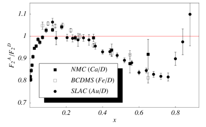
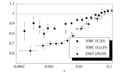
Figure 24: The $x$ dependence of heavy-target/deuteron SFs ratio as measured in DIS of muons and electrons off various nuclear targets and averaged over $Q^{2}$. The left panel shows data from CERN and SLAC for different nuclear targets. The right panel focuses on the region of small $x$ and illustrates nuclear shadowing effect. Data points are from NMC [86], BCDMS [87], SLAC [88] and and FNAL (E665 collaboration [89]) with only statistical errors shown. Nuclear targets are specified in the brackets on the plot legends.

Experimental information about nuclear effects in other DIS observables, such as the ratio of longitudinal to transverse cross sections or the spin SF $g_{1}$, is available but scarse. We note also that DIS off nuclear targets is characterized by additional (new) SFs, which do not appear in DIS off an isolated nucleon. As an example we refer to the tensor SF $b_{1}$, which is specific for spin-1 targets and appears in DIS on deuterium (for a review and references see for instance [85]).

6.1 Nuclear shadowing

Before we turn to the discussion of the DIS regime, it is useful to discuss the low-$Q^{2}$ region away from scaling. Here the behaviour of neutrino cross sections (SFs) is quite different from that of charged leptons. For the latter it is well known that the longitudinal SF $F_{L}$, as well as $F_{2}$, vanish at low $Q^{2}$, because of electromagnetic current conservation. It was shown long ago by Adler that, at low $Q^{2}$, CC neutrino interactions are dominated by the axial current, and neutrino cross sections can be expressed through PCAC in terms of pion cross sections [90]. In contrast to charged-lepton scattering, $F^{\nu}_{L}$ is finite, dominated by a pion pole for $Q^{2}$ at the pion mass scale, and drives the neutrino cross section in this region. Using the Adler relation, Bell predicted nuclear-shadowing effects for neutrino scattering similar to what is observed in pion–nucleus interactions [91]. Going to larger $Q^{2}$ brings a finite contribution from vector and axial-vector meson states, which have been discussed in terms of an extension of the vector meson dominance model to vector and axial-vector currents [92, 93]. Charged-current neutrino interactions with nuclear targets were studied in bubble-chamber experiments [94], where nuclear shadowing was observed at low $Q^{2}$.

Most of the attempts to understand nuclear shadowing are based on the space-time picture of DIS at small $x$ in the target rest frame, where DIS is viewed as the process of interaction of the partonic (or hadronic) component of the exchanged $\gamma^{*}$ or $W^{*}$ with the target. At small $x$ the typical propagation length of those states exceeds the average distance between bound nucleons, and coherent effects in the propagation of partons through the nuclear medium are important. Nuclear shadowing is usually explained by multiple-scattering effects from bound nucleons [85].

Nuclear shadowing in $F_{2}^{\nu}$ was calculated for both low and high $Q^{2}$ regimes in terms of two different models in [95] in an attempt to match muon (NMC) and neutrino (CCFR), data [39] on $F_{2}$ at small $x$. It was found that nuclear shadowing in $F_{2}^{\nu}$ is similar (though slightly smaller in magnitude) to that observed in muon-induced reactions.

At large $Q^{2}$ in the scaling regime both charged-lepton and neutrino-induced reactions are described by universal parton distributions. Some observations on nuclear modifications of different combinations of parton distributions can be made from existing charged-lepton DIS and Drell–Yan data. Phenomenological constraints on the behaviour of nuclear sea and valence quarks at small $x$ were discussed in [100, 101, 102]. Explicit evaluations of nuclear effects in singlet and non-singlet combinations of parton distributions were performed in [103], where nuclear shadowing for $F_{2}^{\nu}$ and $xF_{3}$ was studied in terms of the non-perturbative parton model of [104], which was extended and applied to nuclear targets in [105]. It was found that, while the shadowing effect in neutrino $F_{2}$ is similar to the corresponding effect in charged-lepton DIS, the nuclear shadowing for $xF_{3}$ is enhanced with respect to that for $F_{2}$ in the region of small $x<0.01$ (see Fig. 25). It was argued in [103] that the underlying reason for the enhancement of nuclear shadowing for $xF_{3}$ is its negative $C$-parity. In the small-$x$ region, $xF_{3}$ is determined by the difference of effective quark and antiquark cross sections, and it is known from the multiple-scattering theory that the double-scattering correction to the difference of the cross sections is up to a factor of 2 larger than the corresponding correction to their sum.

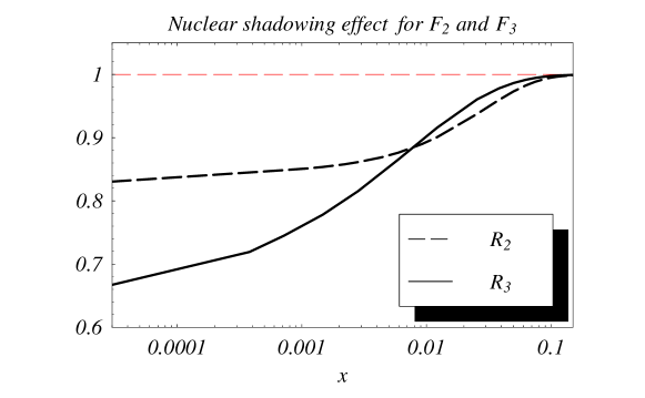
Figure 25: The ratios of a heavy target to the free nucleon SFs $R_{2}=F_{2}^{A}/F_{2}^{N}$ and $R_{3}=F_{3}^{A}/F_{3}^{N}$ calculated for the ⁵⁶Fe nucleus in the region of small $x$ at $Q^{2}=10~{}\rm{GeV}^{2}$ [103]

We note in this respect that a similar enhancement of nuclear shadowing was predicted for the spin SF $g_{1}$ (see discussion in [85]), which involves the differences of quark and antiquark distributions with helicities parallel and antiparallel with respect to the helicity of the target.

6.2 Nuclear effects at large $x$

The physics mechanisms that generate characteristic nuclear effects at large $x$ are quite different from those that govern nuclear shadowing at small $x$. At large $x$ the typical DIS time scale in the laboratory reference frame is small with respect to an average distance between bound nucleons. This allows us to assume that nuclear DIS is dominated by incoherent scattering from bound nucleons. It was found long ago that major nuclear effects here are due to nuclear binding [105, 106, 107], which leads to a depletion of nuclear SFs at $x\sim 0.5$, and to the Fermi motion [108], which is responsible for the enhancement at $x>0.7$. These effects explain the bulk of the observed behaviour of nuclear SFs at $x>0.2$, though detailed understanding of this region is far from complete and further studies of the reaction mechanism are required.

It is quite important to separate nuclear effects in a QCD analysis of neutrino data. As an example we refer to the recent analysis of higher-twist terms in the CCFR data on the $xF_{3}$ SF [109]. The theoretical and experimental situation becomes less clear when going to the region of $x$ close to 1. Here we enter into the resonance region, and the notion of twist expansion becomes less well defined. Nuclear effects in SFs are essential in this region, because the nucleon inelastic SFs must vanish as $x\;\mbox{$\rightarrow$}\;1$. The impact of nuclear effects on HT terms in $xF_{3}$ was studied in [109], where it was shown that the consideration of nuclear effects at large $x$ somewhat decreases the magnitude of dynamical HT terms extracted from CCFR data on iron target. However, the results of calculations of nuclear corrections are sensitive to the details of the nuclear structure input, e.g.  the behaviour of the nuclear spectral function in the region of high excitation energy of the residual nuclear system, which are not known yet. In order to minimize uncertainties associated with nuclear effects, it is desirable to use light nuclear targets in the experiments at the $\nu$-Factory.

We note also that nuclear SFs can extend beyond $x=1$, the kinematical limit for scattering from a free nucleon. Events with $x>1$ have indeed been observed for $F_{2}$ in $\mu$ DIS from a carbon target by the BCDMS collaboration [110] and recently by the CCFR collaboration in neutrino DIS from an iron target [111]. It is rather interesting to search for similar events at the $\nu$-Factory, where the statistics will be much higher.

The region of large $x$ will be explored in more detail in electron scattering experiments at Jefferson Lab. However the experiments at the $\nu$-Factory at large $x$ with different nuclear targets are challenging and could significantly contribute to the field by providing a direct measurement of the EMC effect for different parton combinations, such as the $C$-even $F_{2}$ and $C$-odd $xF_{3}$.

6.3 Nuclear effects in DIS sum rules

As discussed in Section 5.2, the GLS sum rule is a convenient tool to extract $\alpha_{\scriptscriptstyle\mathrm{S}}$ from neutrino data. Neutrino data are usually collected on heavy nuclear targets; therefore, it is of importance to separate contributions to the GLS integral associated with nuclear effects. We denote $S_{\rm GLS}^{A}=S_{\rm GLS}^{N}+\delta S_{\rm GLS}$, where $S_{\rm GLS}^{A}$ and $S_{\rm GLS}^{N}$ are the GLS integral for the nucleus of $A$ nucleons and the isoscalar nucleon respectively, and $\delta S_{\rm GLS}$ accumulates corrections due to nuclear effects. There is a number of effects that can contribute to $\delta S_{\rm GLS}$. Contributions due to nuclear binding, Fermi motion and off-shell effects were discussed in [112]. It was found that these effects cancel out in the leading twist, and a tiny correction appears as a higher twist. For example, $\delta S_{\rm GLS}^{\rm Fe}=-1.2\times 10^{-2}\mathrm{GeV}^{2}/Q^{2}$ and $\delta S_{\rm GLS}^{D}=-1.9\times 10^{-3}\mathrm{GeV}^{2}/Q^{2}$ for the iron and deuterium nuclei respectively. These quantities are more than an order of magnitude smaller than the corresponding QCD power correction estimated in  [75]. However, as was discussed in [103], nuclear shadowing gives a finite and rather large negative correction already in the leading twist. In particular, a $\sim 4\%$ renormalization of the GLS sum rule due to nuclear shadowing was found for the ⁵⁶Fe nucleus, $\delta_{\rm sh}S_{\rm GLS}/S_{\rm GLS}^{N}=-0.035$, at $Q^{2}=10$ GeV².

At this point we must mention that it is usually believed that the GLS sum rule is not renormalized by nuclear effects in the leading in $1/Q^{2}$ order, since to this order the GLS integral counts the baryon number of the target. However, a negative sign of the shadowing correction is also a generic feature of multiple scattering theory. It is therefore challenging to look for a dynamical mechanism that would compensate a negative nuclear shadowing correction in the GLS sum rule. Certainly more work is needed to clarify the status of the GLS sum rule, as well as other DIS sum rules, in nuclear targets.

The Bjorken sum rule for the non-singlet combination of the neutrino SFs $F_{1}$ was discussed in Section 5.3 as an alternative tool to extract $\alpha_{\scriptscriptstyle\mathrm{S}}$. Neutron data are necessary in order to measure this sum rule, and it is clear that, since there exists no free neutron target, nuclear data have to be used. Combined hydrogen and deuterium data are usually used as a source of information about the neutron. The integrated difference between the hydrogen and the deuteron SF could then be used to extract $S_{1}^{d-p}=S_{1}^{n-p}+\delta S_{1}$, where the last term incorporates nuclear effects. Using the method described in [112], it can be shown that the corrections due to nuclear binding and Fermi motion cancel out in the leading twist, similar to the GLS sum rule, and the corresponding power $1/Q^{2}$ correction is small, of the same order of magnitude as in the GLS sum rule.

Note also that the deuteron nucleus, in spite of a weak binding, might not be a perfect source of information about neutron SFs, especially at very large or very small $x$. It was emphasized recently that DIS experiments with mirror ³He and ³H nuclei, which form an isotopic doublet, could give information about the neutron SF practically free from contamination from nuclear effects [113]. We then suggest that the direct measurement of the difference $S_{1}({}^{3}\mbox{He})-S_{1}({}^{3}\mbox{H})$ could be a better source for the Bjorken sum rule than the corresponding hydrogen–deuterium difference. The calculation of corrections to the Bjorken sum rule, as well as to the more fundumental Adler sum rule, due to meson-exchange currents in nuclei and nuclear shadowing, is under way.

In summary we note that because of a larger number of observables, which can be accessed with $\nu$ and $\bar{\nu}$ beams, DIS studies at the $\nu$-Factory can give unique information about the structure of hadrons and nuclei, information that is not accessible with $\mu/e$ machines. In particular, a unique opportunity offered by the $\nu$-Factory is a direct measurement of nuclear sea and valence quarks distributions in a wide kinematical region.

7 ELECTROWEAK STUDIES AT THE $\mathbf{\nu}$-FACTORY

Experiments with $\nu e^{-}$ and $\nu N$ have played a fundamental role in establishing the SM. Before the start of LEP, the best determinations of the electroweak mixing angle came from neutrino experiments, and even now the results from neutrino DIS at NuTeV play an important role in global analyses.

The characteristics of a $\nu$-Factory are such that very precise tests of the SM and its extensions may be possible from neutrino–electron scattering and neutrino induced DIS. As a first approximation, the information available from these experiments can be parametrized in terms of the uncertainty in the determination of the sine of the Weinberg angle, $s_{W}^{2}\equiv\sin^{2}\theta_{W}$. In fact, radiative corrections enter the two processes in different ways and one should look at these experiments as complementary measurements, akin to the present determinations of $\sin^{2}\theta_{\mathrm{eff}}^{\ell}$ and $M_{W}$ at $e^{+}e^{-}$ and hadron colliders. Moreover, a very precise low-energy determination of $s_{W}^{2}$ would test a different variety of new-physics scenarios than usual colliders.

7.1 $\mathbf{\nu e^{-}}$ scattering

$\nu e^{-}$ scattering provides a particularly clean probe of the electroweak coupling. There are several processes which contribute at a $\nu$-Factory:

$$({\rm NC}) \nu_{\mu}e^{-}\mbox{$\rightarrow$}\,\nu_{\mu}e^{-}\;,\ \ \ \bar{\nu}_{\mu}e^{-}\mbox{$\rightarrow$}\,\bar{\nu}_{\mu}e^{-}\;,$$ (54)

$$({\rm NC+CC}) \nu_{e}e^{-}\mbox{$\rightarrow$}\,\nu_{e}e^{-}\;,\ \ \ \bar{\nu}_{e}e^{-}\mbox{$\rightarrow$}\,\bar{\nu}_{e}e^{-},\ \ \ \bar{\nu}_{\mu}\mu^{-}\;,\;\dots\;,$$ (55)

$$({\rm CC}) \nu_{\mu}e^{-}\mbox{$\rightarrow$}\,\nu_{e}\mu^{-}\;.$$ (56)

Events originated by $\nu_{\mu}$ or $\bar{\nu}_{e}$ in a $\mu^{-}$ beam without a muon in the final state cannot be disentangled at a $\nu$-Factory  and must be considered together.

In the case of $\nu e^{-}\mbox{$\rightarrow$}\;\nu e^{-}$ processes, numerical values for the total cross sections are given by

$$\sigma(\nu e^{-}\mbox{$\rightarrow$}\;\nu e^{-})=1.72\times 10^{-41}{\rm cm^{-2}}\times E_{\nu}[\mathrm{GeV}]\times\left[g_{L}^{2}+{1\over 3}g_{R}^{2}\right],$$ (57)

where $g_{L,R}=s_{W}^{2}$ or $g_{L,R}=\pm 1/2+s_{W}^{2}$ according to the process.

Despite the very small cross section, the use of a 2 ton dedicated, fully active target–detector made of liquid CH₄ [3] or of a 20 ton liquid argon [4] time projection chamber should provide around 10⁷ $\nu e$ events/year with a $\mu^{+}$ beam and about half of it with a $\mu^{-}$ beam. In this subsection we use default beam specifications, a 20 cm detector radius, $s_{W}^{2}=0.2314$, and $\int Ldt=8.6\times 10^{46}$ cm^-2.

The signal is a forward electron track with no hadronic activity and energy above a threshold $E_{min}$. The transverse momentum of the outcoming electron is very small, $p_{t}\sim\sqrt{m_{e}E_{\nu}}$. In the configuration considered here the transverse momentum due to the intrinsic divergence of the beam is even smaller. The main source of background is quasi-elastic $\nu_{e}N$ scattering, which can also produce a forward electron, but is characterized by $p_{t}\sim\sqrt{m_{N}E_{\nu}}$ and can be distinguished if the $p_{t}$ resolution of the detector is good. The signal-to-background ratio is expected to be better than 5 at a 50 GeV $\nu$-Factory  [4], leading to a minor dilution of the sensitivities considered below. The $\mu^{-}$ beam has the advantage that quasi-elastic $\nu_{e}N$ scattering produces positrons instead of electrons, so that this source of background can be removed.

Figure 26: (a) statistical uncertainty (in units $10^{-4}$) in the extraction of $\sin^{2}\theta_{W}$ from $\nu e$ scattering as a function of the minimum electron energy. (b) impact of luminosity measurement at the level of $10^{-3}$, 5 $10^{-4}$, 1 $10^{-4}$ on the same $\sin^{2}\theta_{W}$ sensitivities.

The statistical sensitivity to $s_{W}^{2}$ is shown in Fig. 26a as a function of $E_{min}$ for the $\mu^{-}$ and $\mu^{+}$ beams. When only integrated cross sections are considered, the $\mu^{+}$ beam allows for a superior $s_{W}^{2}$ resolution, very close to 1$\times 10^{-4}$, while the $\mu^{-}$ beam is much less sensitive because of a cancellation among different terms. Assuming that a measurement of the outgoing electron energy $E_{e}$ is possible, one can study the $E_{e}$ dependence and achieve a better resolution in the $\mu^{-}$ case, $\delta s_{W}^{2}\approx 2\times 10^{-4}$. This is close to having an optimal observable. For small $E_{min}$, the sensitivity is a mild function of the threshold energy.

A significant problem in $\nu e$ scattering is the normalization of the cross sections. As can be seen from Fig. 26b, in order to preserve the statistical sensitivity one would need a luminosity determination at the level of 10^-4. The goal at a $\nu$-Factory  would be to reach a precision on the flux of $10^{-3}$; this, however, seems inadequate. A realistic possibility is to normalize the $\nu e$ rate to $\nu\mu^{-}$, namely to the muon regeneration process (see Eqs. (55),(56)), which occurs for $E_{\nu}>m_{\mu}^{2}/2m_{e}=10.8$ GeV with cross sections given by

$${d\sigma\over dy}(\bar{\nu}_{e}e^{-}\mbox{$\rightarrow$}\mu^{-}\bar{\nu}_{\mu})={G_{\mu}^{2}\over\pi}s(1-y)\left(1-y+{m_{\mu}^{2}\over s}\right);\ \ \ \ {d\sigma\over dy}(\nu_{\mu}e^{-}\mbox{$\rightarrow$}\mu^{-}\nu_{e})={G_{\mu}^{2}\over\pi}\left(s-m_{\mu}^{2}\right).$$ (58)

Again, the background from $\nu_{\mu}N$ scattering should be considered, but it can be drastically reduced by a cut on the transverse momentum [3]. This mechanism could provide a normalization accuracy of $3.6\times 10^{-4}$, but would be available only for the $\mu^{-}$ beam. On the other hand, it could serve to calibrate different luminosity measurements.

We have also investigated the case in which the muon beams are polarized and concluded that muon polarization would not add significantly to the electroweak measurement. At best, polarization asymmetries could help overcome the normalization problem. With 70% polarized muon beams the statistical error is $\delta s_{W}^{2}\approx 3\times 10^{-4}$ for the $\mu^{-}$ beam, and worse for the $\mu^{+}$ beam. On the other hand, uncertainties in the polarization of the $\mu$ beam do affect the final precision. In order to maintain the final precision at the level of $\delta s_{W}^{2}\approx 10^{-4}$, it is necessary to know the polarization of the muons to 0.05% or better. For this reason precision electroweak measurements require a storage ring design that minimizes these uncertainties.

From the theoretical point of view, all one-loop QED and electroweak corrections are known [115] and could be easily implemented. The uncertainty from higher-order electroweak corrections can be certainly brought below $\delta s_{W}^{2}=1\times 10^{-4}$ [116]. QED corrections to the $e^{-},\mu^{-}$ spectra are relatively important and may need consideration of some higher order effect. A major theoretical uncertainty is likely to come from the hadronic contribution to the $\gamma$–$Z^{0}$ amplitude, which must be calculated at the relevant $Q^{2}\approx 10^{-3}{\rm[GeV]}E_{\nu}$, a region where perturbation theory cannot be applied. The problem is analogous to — but should not be confused with — the one of the hadronic contribution to the running of the electromagnetic coupling, $\Delta\alpha_{hadr}$, which enters most electroweak tests. $\Delta\alpha_{hadr}$ is needed to relate the fine-structure constant $\alpha(q^{2}=0)$ to $\alpha(M_{Z}^{2})$, which is relevant at the $Z^{0}$ pole and for the electroweak corrections to muon decay as well as for low-energy NCs. The latter, however, have an additional sensitivity to hadronic loops in the $\gamma$–$Z^{0}$ mixing. This contribution can be calculated from $e^{+}e^{-}$ data using dispersion relations, SU(3) flavour symmetry, and perturbative QCD. The most recent estimate [117] leads to $\delta s_{W}^{2}=5\times 10^{-4}$. In view of recent progress [118], this can probably be reduced by a factor of 2 or more. However, the use of SU(3) flavour symmetry implies a sizeable ambiguity, which cannot be resolved by better data only. For what concerns the uncertainty in $\Delta\alpha_{hadr}$, it should not be considered a limiting factor for this experiment, as it affects in the same way most electroweak observables. Moreover, there has been and there will be progress in its determination, and it is likely to play a lesser role than the uncertainty from the $\gamma$–$Z^{0}$ mixing in $\nu e$ scattering.

In conclusion, a total uncertainty on $s_{W}^{2}$ of about $2\times 10^{-4}$ is probably achievable at a $\nu$-Factory, in the case where high-performance detectors are available, the polarization of the muons can be controlled very precisely, and progress is achieved in estimating the hadronic effects. Higher precision would require a substantial increase in luminosity as well as major theoretical improvements, mainly in hadronic physics.

7.2 $\mathbf{\sin^{2}\theta_{W}}$ from DIS

Current electroweak analyses of $\nu N$ DIS (at NuTeV) are based on the Paschos–Wolfenstein (PW) relation,

$$R^{-}={\sigma_{NC}({\nu}_{\mu})-\sigma_{NC}(\bar{\nu}_{\mu})\over\sigma_{CC}({\nu}_{\mu})-\sigma_{CC}(\bar{\nu}_{\mu})}={1\over 2}-s^{2}_{W}\;,$$ (59)

which is designed to isolate the $u,d$ valence quark contributions that cancel out in the ratio and is therefore quite insensitive to the hadron structure. On the basis of about 1.3 (0.3) million $\nu_{\mu}$ ($\bar{\nu}_{\mu}$) events, NuTeV has found [119]

$$s_{W}^{2}({\rm OS})=0.2253\pm 0.0019({\rm stat})\pm 0.0010({\rm syst})\pm 0.00025(M_{t})+0.0005\ln{M_{H}\over 150{\rm GeV}}\;.$$ (60)

As can be seen, if the on-shell definition $s^{2}_{W}({\rm OS})\equiv 1-M_{W}^{2}/M_{Z}^{2}$ is used, the indirect dependence of the result on the top and Higgs masses through radiative corrections to Eq. (61) is relatively small. This is why the NuTeV result is often presented as an $M_{W}$ determination with $\delta M_{W}\approx 130$ MeV. This interpretation can be highly misleading when the experimental accuracy reaches ${\cal O}(10^{-4})$.

At a $\nu$-Factory, a striking improvement of the statistical error can be expected, as well as the elimination of the main systematic problems of NuTeV (uncontrolled $\nu_{e}$ beam contamination and NC event identification). Whether the final $s_{W}^{2}$ sensitivity may reach the level of $10^{-4}$ or $\delta M_{W}\approx 5$ MeV depends, however, on many different factors.

If the detector can identify primary $e^{\pm}$ in the final state, the CC events originated by electron neutrinos can be distinguished from NC events. One can then consider ratios of NC/CC total cross sections [3]

$$R^{\mu^{-}}={\sigma_{NC}(\nu_{\mu})+\sigma_{NC}(\bar{\nu}_{e})\over\sigma_{CC}(\nu_{\mu})+\sigma_{CC}(\bar{\nu}_{e})};\ \ \ \ R^{\mu^{+}}={\sigma_{NC}(\bar{\nu}_{\mu})+\sigma_{NC}({\nu}_{e})\over\sigma_{CC}(\bar{\nu}_{\mu})+\sigma_{CC}({\nu}_{e})}$$ (61)

Using our default beam specifications and $E_{lept}>3$ GeV, $E_{h}>1$ GeV, $s^{2}_{W}\equiv\sin^{2}\theta_{W}=0.225$, we find $R^{\mu^{-}}\approx R^{\mu^{+}}=0.36$. Also the $s^{2}_{W}$ sensitivity of the two beams is very similar, $dR/ds^{2}_{W}\approx-0.5$. Because of the $10^{9}$ CC and $3\times 10^{8}$ NC events available for each beam, the statistical error on the $s^{2}_{W}$ determination from Eq. (59) is negligible, as shown in Table 3. However, one should take into account that $R^{\mu^{\pm}}$ have a higher sensitivity to hadronic physics than the PW relation. As an illustration, we show in Table 3 the sensitivity of the $s_{W}^{2}$ determinations from $R^{\mu^{\pm}}$ on present PDFs. The values are obtained by comparing results for $R^{\mu^{\pm}}$ for which different sets of the CTEQ5 PDFs [6] (sets m, d, and hq) have been employed. They are the result of a LO analysis based on present day information. Clearly, future improvements in our knowledge of the hadron structure at the $\nu$-Factory  and elsewhere, as well as a full NLO implementation of QCD radiative corrections will lower this uncertainty, but it seems unlikely that they will bring it down to the level of the statistical error.

On the other hand, the PW relation is formally recovered in the combination

$$(1+g\,r)\,R^{\mu^{-}}-(r+g)\,R^{\mu^{+}},$$ (62)

where $g=\langle E_{\bar{\nu_{e}}}\rangle/\langle E_{\nu_{\mu}}\rangle=0.857$ takes into account the different mean energy of the neutrino and antineutrino beams, $r=\sigma_{CC}(\bar{\nu})/\sigma_{CC}(\nu)$, and lepton universality has been used. Unfortunately, because of the numerical closeness of $R^{\mu^{-}}$ and $R^{\mu^{+}}$, this combination is not an efficient probe. Moreover the $s_{W}^{2}$ sensitivities of $R^{\mu^{\pm}}$ are also very similar and the improvement in the PDF sensitivity is paid for by the lower statistical sensitivity. One possibility is to fit a parameter $\alpha$ in $R^{\mu^{-}}-\alpha R^{\mu^{+}}$ in order to minimize the overall $s_{W}^{2}$ uncertainty. For instance, $\alpha\approx 0.8$ leads to $\delta s_{W}^{2}({\rm PDF})\approx\delta s_{W}^{2}({\rm stat})\approx 0.0002$.

Observable	Stat. error	PDF
$R^{\mu^{-}}$	0.4	$\sim$ 12
$R^{\mu^{+}}$	0.5	$\sim$ 15
$R^{\mu^{-}}-0.8R^{\mu^{+}}$	2.2	$\sim 2$
$P$	4.9	$\sim$ 4

Table 3: Uncertainties on the $s^{2}_{W}$ determination from different observables in $\nu$ DIS in units $10^{-4}$ (see text).

Of course, one can construct other ratios of cross sections, also combining the cross sections of the two beams in a way similar to Eq. (59); however, they tend to be less sensitive to $s^{2}_{W}$ and/or to depend even more than $R^{\mu^{\pm}}$ on the hadronic structure. A possible exception could be the quantity

$$P={\sigma_{NC}(\mu^{-})-\sigma_{NC}(\mu^{+})\over\sigma_{CC}(\mu^{-})-\sigma_{CC}(\mu^{+})}\;,$$ (63)

which is modelled on the PW relation and has indeed a lower sensitivity on hadronic physics (see Table 3). However, this observable is penalized by a lower $s_{W}^{2}$ resolution and requires the knowledge of the ratio $\sigma_{CC}(\mu^{+})/\sigma_{CC}(\mu^{-})$ — and therefore of the relative normalization of the two beams — to better than $10^{-4}$.

These high-precision measurements cannot be carried out without a high-performance tracking target. The detector and beam requirements based on Eqs. (61) have been discussed in [3]. The main ones are high electron/muon detection efficiency, good primary lepton identification, and precise momentum and energy measurements. A rough estimate [3] of the corresponding uncertainties is $\delta s_{W}^{2}\approx 2\times 10^{-4}$. The ability to have both $\mu^{+}$ and $\mu^{-}$ beams would be an important asset, as it would allow the use of Eq. (62).

From a theoretical point of view, it will be necessary to implement full NLO QCD and QED corrections, to incorporate possibly complete two-loop electroweak corrections, to assess the importance of higher twists, and to take into account charm production corrections. This is to be contrasted with the obsolete and incomplete implementation of QCD and electroweak corrections of the NuTeV analysis. On the other hand, almost all theoretical tools are in principle already available, including the dominant two–loop weak corrections [116]. Charm production, in particular, is likely to be a significant source of uncertainty; it accounts for about 3% of the total CC cross section and therefore even a 1% error on the overall charm yield would induce a $10^{-4}$ uncertainty on $R^{\mu^{\pm}}$ or $\delta s_{W}^{2}\approx 2\times 10^{-4}$. An extrapolation from the CCFR measurements suggests $\delta s_{W}^{2}\sim 0.0003$ [3].

If the outcoming electrons cannot be resolved and CC events initiated by electron neutrinos are considered as NC events — a situation analogous to present-day $\nu N$ experiments — the only observable for the $\mu^{-}$ beam is

$$\hat{R}^{\mu^{-}}={\sigma_{NC}(\nu_{\mu})+\sigma_{NC}(\bar{\nu}_{e})+\sigma_{CC}(\bar{\nu}_{e})\over\sigma_{CC}(\nu_{\mu})}\;.$$ (64)

This observable and the analogous one for the $\mu^{+}$ beam have a marginally lower statistical sensitivity and a much higher dependence on the SFs, $\delta s_{W}^{2}>0.02$, than $R^{\mu^{\pm}}$.

In conclusion, efficient electron identification seems to be crucial for a very precise determination of $s^{2}_{W}$ at the $\nu$-Factory . The statistical uncertainties are likely to be negligible in comparison with theoretical and experimental systematic errors, which in turn are difficult to estimate at the moment. Before a realistic assessment of the potential of $\nu$ DIS at a $\nu$-Factory for precision electroweak tests is possible, several systematics will have to be understood; most importantly the precision of the $\nu$-Factory measurement of the unpolarized SFs, primary lepton identification, isospin–violating effects and charm production.

7.3 New physics through radiative corrections

The very precise determination of the electroweak mixing angle from $\nu e$ and $\nu N$ scattering at a $\nu$-Factory would test the SM at a level competitive with LEP, SLD and Tevatron measurements. Experiments at the front end of a muon storage ring could therefore severely constrain many extensions of the SM, which potentially affect the SM predictions for neutrino scattering through virtual contributions. If the new physics is characterized by a high mass scale and it affects dominantly the two-point functions, its contributions can be parametrized in a model independent way by the $S,T,U$ amplitudes introduced in [120]. Similar strategies have been presented by a number of authors (see for instance [121]). Many models of physics beyond the SM can be studied at least approximately in this simple way.

We use $M_{H}\approx 100$ GeV and $\hat{s}_{W}^{2}=\sin^{2}\theta_{W}(M_{Z})_{\overline{\rm MS}}=0.2315$ as reference SM values and set $g=\langle E_{\bar{\nu_{e}}}\rangle/\langle E_{\nu_{\mu}}\rangle=0.857$. As far as $\nu e$ scattering is concerned, in the case of the $\mu^{-}$ beam we can consider the ratio of electron- and muon-production total cross sections

$$r^{-}={\sigma(\nu e^{-})\over\sigma(\nu\mu^{-})}\;.$$ (65)

Virtual effects parametrized by $S$, $T$, and $U$ shift the measured value of $r$ with respect to the SM prediction $r_{0}$ by

$$r^{-}=r^{-}_{0}\,(1+0.0055\,S+0.0004\,T)\;.$$ (66)

This observable is therefore very insensitive to the isospin breaking parameter $T$, similarly to the weak charge in atomic parity violation experiments with cesium. It could allow for a very accurate determination of the isospin conserving parameter $S$, within $\pm 0.1$; this is roughly the accuracy of the present global fit (see Ref. [122], p.105). A similar observable can be constructed for the $\mu^{+}$ beam, provided the luminosity determination is based on a CC process analogous to muon production. In this case the shift is

$$r^{+}=r^{+}_{0}\,(1+0.0111\,S-0.0100\,T)\;,$$ (67)

and implies a very different constraint in the $(S,T)$ plane. Finally, the measured value of the Paschos–Wolfenstein relation (59) is affected by the oblique parameters according to

$$R^{-}=R^{-}_{0}\,(1-0.0136\,S+0.0253\,T)$$ (68)

The different $\nu e$ and $\nu N$ measurements would therefore provide complementary constraints on new physics.

8 STUDIES WITH HEAVY QUARKS

As has been pointed out in the past, and as shown in a previous section, the $\nu$-Factory can be seen as a $\nu$DIS charm factory. A comprehensive review of the possible physics goals of such a facility can be found in Ref. [3]. Here we shall explore in quantitative detail some interesting example, drawing from the expertise available within the Working Group. In particular we shall focus on two aspects of charm production in neutrino interactions: low-multiplicity processes such as the diffractive $D_{s}$ and the quasi-elastic charmed-baryon production. We shall show that these processes allow a clear identification of the charmed hadron, and therefore a very good estimate of absolute decay branching ratios. Together with low systematic errors, these measurements can provide, for instance, a precise measurement of $f_{D_{s}}$.

In the following we consider nuclear emulsions both as neutrino target and tracking device. It is worth stressing that the use of nuclear emulsions is limited by the overlapping of interactions. A density of interactions of about $20$ per cm³ is reasonable. On the other hand, $10^{7}~{}\nu_{\mu}$ interactions are needed for the measurements we will discuss in the following. Such a statistics could be obtained by running the machine at low luminosity and taking data for a few years (months) whether the experiment is located far from ($\mathcal{O}(1~{}\mbox{km})$) or close to ($\mathcal{O}(100~{}\mbox{m})$) the neutrino source.

Our simulations include realistic estimates of the experimental efficiencies and systematics. It is important to point out, however, that the methods discussed below can be used by electronic experiments with a very good vertex detector as well, although with different efficiencies and backgrounds.

8.1 Direct evaluation of the $\mathbf{\Lambda}_{c}^{+}$ branching ratios

8.1.1 Model-independent extraction of $BR(\Lambda_{c}^{+}\rightarrow pK^{-}\pi^{+})$

So far, only model-dependent extractions of $\Lambda_{c}^{+}$ branching ratios have been obtained, see [122]. A method, based on the neutrino quasi-elastic charm production, for a model-independent determination of most of the $\Lambda_{c}^{+}$ branching ratios has been proposed in Ref. [123]. So far, two different methods to extract $\Lambda_{c}^{+}$ branching ratios have been used [122]. As discussed in Ref. [122] they rely on different theoretical assumptions on $B$ physics, namely the $B$ branching ratios to $\Lambda_{c}$, and give results that are not in quite a good agreement. Therefore, a model-independent determination of $\Lambda_{c}^{+}$ branching ratios would provide a better theoretical understanding of the baryonic $b$-decays. For a detailed discussion of this method, see Ref. [123].

8.1.2 Present knowledge, theoretical and experimental, of neutrino quasi-elastic charm production

The simplest exclusive charm-production reaction is the quasi-elastic process where a $d$ valence quark is changed into a $c$ quark, thus transforming the target nucleon into a charmed baryon. Explicitly, the quasi-elastic reactions are

$$\nu_{\mu}n\rightarrow\mu^{-}\Lambda_{c}^{+}(2285)\;,\nu_{\mu}n\rightarrow\mu^{-}\Sigma_{c}^{+}(2455)\;,\nu_{\mu}n\rightarrow\mu^{-}\Sigma_{c}^{*+}(2520)\;,$$ (69)

$$\nu_{\mu}p\rightarrow\mu^{-}\Sigma_{c}^{++}(2455)\;,\nu_{\mu}p\rightarrow\mu^{-}\Sigma_{c}^{*++}(2520)\;.$$ (70)

For a detailed theoretical review of neutrino quasi-elastic charm production, see Refs.[124]–[130].

The predicted cross sections, assuming a neutrino energy of $10$ GeV and according to different authors, are shown in Table 4. As we can see, these predictions can even differ by one order of magnitude. If we express the total quasi-elastic charm production rate with respect to deep-inelastic CC interactions, it ranges from $0.33\%$ to $9.0\%$ (see Table 4). From Fig. 3 of Refs. [125] and [130] we note that the total cross section in both models is almost flat for neutrino energies above $8$ GeV.

$\sigma(10^{-40}~{}\mbox{cm}^{2})\backslash$ Model	F.R. [124]	S.L. [125]	A.K.K. [126, 127, 128]	A.G.Y.O. [129]	K. [130]
$\nu_{\mu}p\rightarrow\mu^{-}\Sigma_{c}^{++}$	$0.2(0.030\%)$	$9.0(1.3\%)$	$8.0(1.2\%)$	$1.0(0.15\%)$	$3.0(0.45\%)$
$\nu_{\mu}p\rightarrow\mu^{-}\Sigma_{c}^{*++}$	$0.6(0.089\%)$	$16.0(2.4\%)$	$10.0(1.5\%)$	$0.6(0.089\%)$	-
$\nu_{\mu}n\rightarrow\mu^{-}\Lambda_{c}^{+}$	$1.0(0.15\%)$	$23.0(3.4\%)$	$41.0(6.1\%)$	$3.0(0.45\%)$	$5.0(0.74\%)$
$\nu_{\mu}n\rightarrow\mu^{-}\Sigma_{c}^{+}$	$0.1(0.015\%)$	$5.0(0.74\%)$	-	$0.6(0.089\%)$	$1.5(0.22\%)$
$\nu_{\mu}n\rightarrow\mu^{-}\Sigma_{c}^{*+}$	$0.3(0.045\%)$	$8.0(1.2\%)$	-	$0.3(0.045\%)$	-
Total	$2.2(0.33\%)$	$61.0(9.0\%)$	$59.0(8.9\%)$	$5.5(0.82\%)$	$9.5(1.41\%)$

Table 4: Predicted quasi-elastic charm-production cross section assuming a neutrino energy of $10$ GeV. In brackets the quasi-elastic charm rate with respect to deep-inelastic interactions is given.

The statistics of neutrino quasi-elastic charm events collected by bubble chamber and emulsion experiments is rather poor. The measured cross sections, obtained by a reanalysis that uses the latest results on $\Lambda_{c}^{+}$ branching ratios [122], are shown in Table 5.

Experiment	$\sigma_{\Sigma_{c}^{++}}$	$\sigma_{\Sigma_{c}^{*++}}$	$\sigma_{\Lambda_{c}^{+}}$	$(\sigma_{\Lambda_{c}^{+}}+\sigma_{\Sigma_{c}^{+}}+\sigma_{\Sigma_{c}^{*+}})$	$(\sigma_{\Sigma_{c}^{++}}+\sigma_{\Sigma_{c}^{*++}})$
	$(10^{-40}~{}\mbox{cm}^{2})$	$(10^{-40}~{}\mbox{cm}^{2})$	$(10^{-40}~{}\mbox{cm}^{2})$	$(10^{-40}~{}\mbox{cm}^{2})$	$(10^{-40}~{}\mbox{cm}^{2})$
[131]	$(2.3^{+2.7}_{-1.6})$
[132]	$(2.3\pm 2.0)$	$(4.5\pm 4.0)$
[133]			$(0.9^{+0.9}_{-0.7})$
[134]			$(3.7^{+3.7}_{-2.3})$
[135]				$(38.3\pm 23.1)$	$<8.8$
Average	$(2.3\pm 1.5)$	$(4.5\pm 4.0)$	$(1.1\pm 0.8)$	$(38.3\pm 23.1)$	$<8.8$

Table 5: Summary of the experimental measurements of quasi-elastic charm-production cross sections.

Despite the large statistical error, these measurements are clearly inconsistent with the predictions of Refs. [125]–[128], while the agreement is fair for the ones in Refs. [124, 129, 130]. The average value of the cross sections predicted by Refs. [124, 129, 130] has been used to get a rough estimate of the expected number of events, given in Table 6.

Reaction	$\sigma(10^{-39}~{}\mbox{cm}^{2})$	$\mathcal{R}(\%)$	Expected events
$\nu_{\mu}p\rightarrow\mu^{-}\Sigma_{c}^{++}$	0.14	$0.14$	14000
$\nu_{\mu}p\rightarrow\mu^{-}\Sigma_{c}^{*++}$	0.06	$0.06$	6000
$\nu_{\mu}n\rightarrow\mu^{-}\Lambda_{c}^{+}$	0.3	$0.3$	30000
$\nu_{\mu}n\rightarrow\mu^{-}\Sigma_{c}^{+}$	0.07	$0.07$	7000
$\nu_{\mu}n\rightarrow\mu^{-}\Sigma_{c}^{*+}$	0.03	$0.03$	3000
All	0.6	$0.6$	60000

Table 6: Quasi-elastic charm-production cross section and its contribution to the total CC neutrino cross section. The last column shows the expected number of events, assuming a starting sample of $10^{7}$ CC neutrino-induced events.

8.1.3 Description of the method

The method consists in identifying the $\Lambda_{c}$ by means of the peculiar topology of the quasi-elastic reaction. As shown in Fig. 27, the only charged particles produced in this process are the muon and the short-lived particle ($\Lambda_{c}$) except for the reaction Fig. 27c) where an additional $\pi$ is produced. Therefore there is only a small contamination of these events from deep-inelastic charm production where a charmed hadron is produced (faking a $\Lambda_{c}$) and the topology is quasi-elastic-like.

In this way, since we only use topological information, the $\Lambda_{c}$ identification is model-independent. The relative contamination of $D^{+}$ and $D^{+}_{s}$ from deep-inelastic events, $\varepsilon_{fake}$, can be dealt with as a relative systematic error on the branching ratios. We assume the relative systematic error to be $\varepsilon_{fake}+3\sigma_{fake}$ where $\sigma_{fake}$ is the error on $\varepsilon_{fake}$ .

The normalization to determine the $\Lambda_{c}^{+}$ absolute branching ratios is simply given by the number of events with a vertex topology consistent with Fig. 27. No model-dependent information is used to define the normalization. The little knowledge we have about the quasi-elastic charm-production cross section, which is model-dependent unless measured, plays a role only in the evaluation of the deep-inelastic contamination, namely the systematic error. In fact, in the evaluation of the contamination, the ratio $\mathcal{R}$ between charm quasi-elastic and standard deep-inelastic production appears. It is worth noting that, even if the ratio $\mathcal{R}$ had an uncertainty of $500\%$, the relative systematic error on the branching ratios would be $\sim 7.2\%$ (see [123]).

Figure 27: Topology of the quasi-elastic neutrino-induced charm events in the case of the reactions a) $\nu_{\mu}n\rightarrow\mu^{-}\Lambda_{c}^{+}$, b) $\nu_{\mu}n\rightarrow\mu^{-}\Sigma_{c}^{+}(\Sigma_{c}^{*+})$ and c) $\nu_{\mu}p\rightarrow\mu^{-}\Sigma_{c}^{++}(\Sigma_{c}^{*++})$, with subsequent $\Sigma_{c}$ decay into $\Lambda_{c}$. The particles inside the box represent the $\Lambda_{c}^{+}$ decay products.

8.1.4 Measurement accuracy

Channel	PDG BR [122]	$\Delta BR$	$\Delta BR$	$\Delta BR$
		(${\Delta\mathcal{R}\over\mathcal{R}}=10\%$)	(${\Delta\mathcal{R}\over\mathcal{R}}=100\%$)	(${\Delta\mathcal{R}\over\mathcal{R}}=500\%$)
$\Lambda_{c}^{+}\rightarrow pK^{-}\pi^{+}$	$(5.0{\pm}1.3)\%$	$({\pm}0.09{\pm}0.04)\%$	$({\pm}0.09{\pm}0.09)\%$	$({\pm}0.09{\pm}0.4)\%$
$\Lambda_{c}^{+}\rightarrow\Lambda\mu^{+}\nu_{\mu}$	$(2.0{\pm}0.7)\%$	$({\pm}0.06{\pm}0.01)\%$	$({\pm}0.06{\pm}0.04)\%$	$({\pm}0.06{\pm}0.1)\%$
$\Lambda_{c}^{+}\rightarrow\Lambda e^{+}\nu_{e}$	$(2.1{\pm}0.7)\%$	$({\pm}0.06{\pm}0.01)\%$	$({\pm}0.06{\pm}0.04)\%$	$({\pm}0.06{\pm}0.1)\%$

Table 7: Statistical and systematic accuracy achievable in the determination of the $\Lambda_{c}^{+}$ absolute branching ratios, assuming a collected statistics of $10^{7}~{}\nu_{\mu}$ CC events, as a function of the relative error on $\mathcal{R}$. The central values are taken from Ref. [122].

The expected accuracy on the determination of the $\Lambda_{c}^{+}$ branching ratios as a function of the relative error on $\mathcal{R}$, the quasi-elastic charm production cross section relative to the deep-inelastic one, is shown in Table 7. To compute the expected number of events in each decay channel we use the central values (shown in Table 7 together with their errors) given by the Particle Data Group [122]. From this table we can see that, even assuming a very large (unrealistic) systematic error, the achievable accuracy on the branching ratios makes the discrimination between the methods discussed in Ref. [122] still possible.

8.2 Direct evaluation of $\mathbf{D}_{s}$ branching ratios and $\mathbf{f}_{D_{s}}$ measurement

The experimental knowledge on leptonic $D_{s}$ decays is very little. Currently, the branching ratios for $D_{s}\rightarrow l\nu$ decays have been estimated by the PDG [122] to be $BR(D_{s}\rightarrow\mu\nu)=(4.6\pm 1.9)\times 10^{-3}$ and $BR(D_{s}\rightarrow\tau\nu)=(7\pm 4)\times 10^{-2}$. These large uncertainties translate into a large uncertainty on the extraction of the decay constant $f_{D_{s}}$.

A method that would allow at the $\nu$-Factory the extraction of most of the $D_{s}$ branching ratios, and consequently of $f_{D_{s}}$, by means of purely leptonic decays, has been proposed in Ref. [136]; the expected accuracy would be better than $5\%$. Once $f_{D_{s}}$ will be measured with such an accuracy, one will feel more confident about extrapolating to the decay constants in the $B$ system, $f_{B}$ and $f_{B_{s}}$, which are crucial quantities for the quantitative understanding of $B^{0}_{(s)}$–$\bar{B}^{0}_{(s)}$ oscillations and the extraction of $V_{td}$ ($V_{ts}$) from them.

8.2.1 Topology of neutrino-induced diffractive charm events and background

In $D_{s}^{(*)}$ diffractive production, only a muon is produced at the interaction point (primary vertex), besides the charmed meson. Therefore, these events are characterized by a peculiar topology: two charged tracks at the primary vertex, one of them being a short-lived particle.

Neutrino-induced quasi-elastic charm events are characterized by the topologies shown in Fig. 27. Therefore, they are similar to the diffractive ones, but with a cross section twice as large. Since antineutrinos cannot induce quasi-elastic charm production, while diffractive production is the same for both $\nu$ and $\bar{\nu}$, in the following we will consider only $\bar{\nu}$ beams. We will then make the assumption that all the events with the above topology are due to $D_{s}^{(*)}$ diffractive production. In this case we will wrongly classify some of the charmed hadrons produced in deep-inelastic interactions.

The charm production in $\bar{\nu}$ interactions and the event topology have been studied by using the HERWIG event generator [137], as well as an event generator based on JETSET [138] and LEPTO [139], assuming the energy dependence of the charm fractions reported in [140]. The average charm fractions, convoluted with the neutrino spectrum, are $F_{\bar{D}^{0}}=61\%$, $F_{{D}^{-}}=26\%$, $F_{{D}^{-}_{s}}=7.3\%$ and $F_{{\Lambda}^{-}_{c}}=5.7\%$.

The signal kinematics has been studied by using an event generator developed within the CHORUS Collaboration [141].

The contamination to the diffractive sample, which comes from deep-inelastic events, can be written as

$$\varepsilon_{fake}={\sigma(\bar{\nu}_{\mu}N\rightarrow\mu^{+}CX)\over\sigma(\bar{\nu}_{\mu}N\rightarrow\mu^{+}X)}{\times}{1\over\bar{\mathcal{R}}}{\times}(F_{D^{-}}+F_{\Lambda_{c}^{-}})\times f_{fake}{\times}\varepsilon_{kin}$$ (71)

where

$$\bar{\mathcal{R}}\equiv{\sigma(\bar{\nu}_{\mu}N\rightarrow\mu^{+}D_{s}^{(*)-}N)\over\sigma(\bar{\nu}_{\mu}N\rightarrow\mu^{+}X)}\,.$$ (72)

We take the charm production in $\bar{\nu}$ interaction to be $3\%$ [142]. By using the charm fractions discussed above, $(F_{D^{-}}+F_{\Lambda_{c}^{-}})=31.7\%$. The factor $f_{fake}=(6.0\pm 0.1)\%$ is the fraction of deep-inelastic charmed events faking the diffractive topology; $\varepsilon_{kin}=(0.4\pm 0.2)\%$ gives the efficiency of kinematical cuts as explained in Ref. [136]. Finally we get $\varepsilon_{fake}\simeq 0.04\%$.

The currently measured $\bar{\mathcal{R}}$ has an error of about $15\%$ (see Ref. [136]), which affects the relative error on $\varepsilon_{fake}$. As described in Ref. [136], a kinematical analysis allows a good $D_{s}$ detection efficiency ($\sim 73\%$) with a small background. The expected contamination and its error are given in Table 8.

Another possible source of irreducible background is the diffractive production of $D^{(*)-}$ (see Ref. [136]). It is suppressed by a factor $\left|V_{cs}/V_{cd}\right|^{2}\sim 20$ and only $30\%$ of the $D^{*-}$ decay into a charged charmed meson ($BR(D^{*-}\rightarrow D^{-})=0.323\pm 0.006$ [122]). On the other hand, all the diffractively produced $D^{-}$ are background: we assume that $D^{-}$ are half of the diffractive sample . Finally, we get $\varepsilon_{D^{*}}=(3.3\pm 0.8)\%$.

From the numbers given above, it turns out that the little knowledge we have about the diffractive charm production cross-section plays a role only in the evaluation of the deep-inelastic contamination, namely a term of the systematic error. Even if the ratio $\bar{\mathcal{R}}$ had an uncertainty of $100\%$, the relative systematic error on the branching ratios would be $\sim 0.04\%$ (see Table 8). We want to stress that, since the $\varepsilon_{D^{(*)}}$ contribution is dominant, the overall systematic uncertainty does not depend at all on the $\bar{\mathcal{R}}$ accuracy. Writing the relative systematic error from deep-inelastic events as $\varepsilon_{fake}+3\sigma_{fake}$, where $\sigma_{fake}$ is the error on $\varepsilon_{fake}$, the overall relative systematic uncertainty is

$$\varepsilon_{sys}=\sqrt{(\varepsilon_{fake}+3\sigma_{fake})^{2}+\varepsilon_{D^{(*)}}^{2}}=(3.3\pm 0.8)\%\;,$$ (73)

which is dominated by the $\varepsilon_{D^{(*)}}$ term.

$\Delta\bar{\mathcal{R}}/\bar{\mathcal{R}}$	$\sigma_{fake}/\varepsilon_{fake}$	$\varepsilon_{fake}(\%)$	$\varepsilon_{D^{(*)}}(\%)$
$15\%$	$23\%$	$0.037{\pm}0.009$	$3.3\pm 0.8$
$30\%$	$34\%$	$0.04{\pm}0.01$	$3.3\pm 0.8$
$50\%$	$53\%$	$0.04{\pm}0.02$	$3.3\pm 0.8$
$100\%$	$101\%$	$0.04{\pm}0.04$	$3.3\pm 0.8$

Table 8: The relative and absolute error on $\varepsilon_{fake}$ as a function of the relative error on $\bar{\mathcal{R}}$. In the fourth column the systematic uncertainty due to the $D^{(*)}$ contamination is reported.

8.2.2 Description of the method

An almost pure sample of $D_{s}^{-}$ from diffractive events, with a small contamination of $D^{-}$ and $\Lambda_{c}^{-}$ produced in deep-inelastic events and in diffractive $D^{(*)-}$ production, can be built by using diffractive $D_{s}^{(*)}$ production from antineutrinos. The normalization to determine the $D_{s}$ absolute branching ratios is given by the number of events with a vertex topology consistent with one $\mu$ plus a short-lived particle. No model-dependent information is used to define the normalization.

It is worth noting that the contamination of $D^{-}$ and $\Lambda_{c}^{-}$ events does not affect the $D_{s}\rightarrow\tau$ channel. Indeed, such events would present a unique topology with two subsequent kinks. An event with a double kink has been observed recently in CHORUS (see Ref. [141]).

8.2.3 Measurement accuracy at a neutrino factory

At present there are no experiments with both an adequate spatial resolution to fully exploit the diffractive topology and a sufficient antineutrino-induced CC event statistics. Therefore, the method proposed in this paper could only be exploited with the above-mentioned detector exposed at a $\nu$-Factory.

Let us assume that $10^{7}$ $\bar{\nu}$ CC events are collected into an emulsion target and that the detection efficiency is about $73\%$ for the $D_{s}$ decays. By assuming a vertex location efficiency of about $50\%$ and assuming a $\bar{\nu}$ diffractive production rate of $6.2\times 10^{-3}$/CC event, we expect to detect a number of $D_{s}$ equal to $N_{D_{s}}=10^{7}\times 6.2\times 10^{-3}\times 0.73\times 0.5\simeq 2.3\times 10^{4}$.

The expected accuracy on the determination of the $D_{s}$ branching ratios is shown in Table 9 for a few channels, together with the current status. To compute the expected number of events in each decay channel we have used the central values (shown in Table 9 together with their errors) given by the Particle Data Group [122].

Channel	PDG BR [122]	New method
$D_{s}\rightarrow\mu\nu$	$(4.6\pm 1.9)\times 10^{-3}$	$({\pm}0.55{\pm}0.15)\times 10^{-3}$
$D_{s}\rightarrow\tau\nu$	$(7\pm 4)\%$	$({\pm}0.17{\pm}0.23)\%$
$D_{s}\rightarrow\phi l\nu$	$(2.0\pm 0.5)\%$	$({\pm}0.08{\pm}0.07)\%$

Table 9: Statistical and systematic accuracy achievable in the determination of the $D_{s}$ absolute branching ratios, assuming a collected statistics of $10^{7}~{}\bar{\nu}_{\mu}$ CC events. The central values are taken from Ref. [122].

As discussed in Ref. [145] the leptonic branching ratios are proportional to the decay constant. Therefore, by using the measured branching ratios given in Table 9, $f_{D_{s}}$ can be extracted. If we collect $10^{7}$ $\bar{\nu}_{\mu}$ CC interactions we get $f_{D_{s}}=288\pm 4(\mathrm{stat})\pm 5(\mathrm{syst})$ MeV, where the central value is taken from Ref. [122].

8.3 Theoretical estimates for $\mathbf{\nu}$-induced exclusive $\mathbf{D}_{s}$ production

The observation of exclusive $D_{s}$ production at the $\nu$-Factory, through the process $\bar{\nu}_{\mu}+N\mbox{$\rightarrow$}\;\mu^{+}+N+D_{s}^{-}$, is also of interest for the study of the production mechanism within QCD and opens a new possibility to study the nucleon structure. There exists a QCD factorization theorem [146, 147], which states that the amplitude for hard exclusive meson-production processes can be written as a convolution of a skewed parton distribution (SPD), a distribution amplitude, and a hard part. This theorem has recently been applied to the investigation of electroproduction of single light mesons [148] and meson pairs [149]. Motivated by the possible implications for the $\nu$-Factory, the formalism has been extended to CC-induced processes. We summarize here the main results of this work, whose validity is limited to values of $Q^{2}$ large compared to $-t$ and to the squared masses of the involved particles. The differential cross section of the leptoproduction process is given by

$${\mathrm{d}\sigma\over\mathrm{d}x_{\mathrm{Bj}}\mathrm{d}Q^{2}\mathrm{d}t}={e^{2}\over 4(4\pi)^{3}\sin^{2}\theta_{W}}{x_{\mathrm{Bj}}\over Q^{2}(Q^{2}+M_{W}^{2})^{2}}\biggl{(}1-{Q^{2}\over 2x_{\mathrm{Bj}}\,p\cdot l}\biggr{)}\sum_{s^{\prime}}|T|^{2}\;,$$ (74)

where $l$ is the neutrino momentum and $T$ is the amplitude for the subprocess

$$W^{-^{\ast}}_{L}(q)+N(p)\mbox{$\rightarrow$}D_{s}^{-}(q^{\prime})+N(p^{\prime})\;.$$ (75)

At leading order, $T$ is obtained from the sum of three diagrams involving a gluon SPD (Fig. 28a and diagrams obtained by an interchange of the order of the vertices) and two diagrams with a contribution of the (polarized and unpolarized) strange quark SPD (Fig. 28b plus one diagram with a changed order of vertices).

Figure 28: Two of the five contributing diagrams.

The relative Feynman diagrams are convoluted with the gluon and $s$ quark SPD and with the distribution amplitude $\Phi_{D_{s}^{-}}(z)$ for the $D_{s}^{-}$ meson ($z$ being the fraction of the $D_{s}^{-}$ momentum carried by the strange quark).

For a numerical estimate of the cross section we adopt the distribution amplitude from [150]:

$$\Phi_{D_{s}^{-}}(z)=N_{D_{s}}\sqrt{z(1-z)}\exp\bigg{[}-{m_{D_{s}}^{2}\over 2\omega^{2}}z^{2}\bigg{]}\;,$$ (76)

where $\omega=1.38\,\mathrm{GeV}$ was obtained in [151] as the best fit for the $D$ meson, and $N_{D_{s}}$ has to be chosen to satisfy the sum rule

$$\int_{0}^{1}\mathrm{d}z\,\Phi_{D_{s}^{-}}(z)=f_{D_{s}}$$ (77)

For a comparison, we shall also use the asymptotic form of the $D_{s}$ distribution amplitude:

$$\Phi_{D_{s}^{-}}(z)=6f_{D_{s}}z(1-z)\;.$$ (78)

In both cases we use $f_{D_{s}}=270\,\mathrm{MeV}$, namely the average of the results obtained so far in lattice calculations [152]. The gluon and quark SPD’s are parameterized as in [149], combining Radyushkin’s model [147, 153] with the parameterizations of the usual (forward) parton distributions of Ref. [154].

Figure 29 shows the results obtained for the differential cross sections $\mathrm{d}\sigma/\mathrm{d}x_{\mathrm{Bj}}$ and $\mathrm{d}\sigma/\mathrm{d}Q^{2}$ where $t=(p-p^{\prime})^{2}$ has been integrated over the interval $t_{\mathrm{min}}=m_{N}^{2}x_{\mathrm{Bj}}^{2}/(1-x_{\mathrm{Bj}})<-t<2\,\mathrm{GeV}^{2}$, assuming for simplicity a fixed neutrino energy $E_{\bar{\nu}}=34\,\mathrm{GeV}$. For the plot of the $x_{\mathrm{Bj}}$-dependence $Q^{2}$ has been integrated from $12\,\mathrm{GeV}^{2}$ to the upper bound given by the constraint $y<1$, with $y:=p\cdot q/p\cdot l=Q^{2}/(2x_{\mathrm{Bj}}p\cdot l)$. The plot of $\mathrm{d}\sigma/\mathrm{d}Q^{2}$ is based on the $x_{\mathrm{Bj}}$-integrated cross section, integrated between $x_{\mathrm{Bj}}=0.18$ and $x_{\mathrm{Bj}}=0.75$ and taking into account the same kinematical constraint. The solid lines correspond to the form of $\Phi_{D_{s}^{-}}$ given in Eq. (77), while the dashed lines correspond to the asymptotic form of Eq. (78).

         

Figure 29: The differential cross section for exclusive $D_{s}^{-}$ production as a function of $x_{\mathrm{Bj}}$ or $Q^{2}$ respectively. The dotted lines show the contribution stemming from the gluon SPD. The results obtained for the asymptotic form of the distribution amplitude $\Phi_{D_{s}^{-}}$ are plotted with dashed lines.

The dotted lines are obtained by setting to zero the strange quark SPD, proving the dominance of the gluon contribution, and suggesting that this process is a potential probe for the measurement of the gluon SPD.

Integrating over all variables $Q^{2}$, $x_{\mathrm{Bj}}$, and $t$ over the same kinematical region gives a value for the total cross section of $\sigma=5.6\times 10^{-14}\,\mathrm{GeV}^{-2}=2.2\times 10^{-5}\,\mathrm{pb}$. Uncertainties of this rough estimate result from the current limited knowledge of the SPDs, by the 20% uncertainty on $f_{D_{s}}$, and by the lack of knowledge about the exact form of the meson-distribution amplitude, as illustrated in Fig. 29. It is worth noting, however, that experiments of the kind discussed here can provide much more precise information on the $D_{s}$ decay constant independently of the exact cross section. As discussed in the previous subsection the relatively high production rate of $D_{s}$ mesons allows us to determine $f_{D_{s}}$ by measuring the $D_{s}$ branching ratios and its total width [136]. In spite of the small cross section, the huge integrated luminosities of $\int L\mathrm{d}t>10^{9}\,\mathrm{pb}^{-1}$ available at the $\nu$-Factory would lead to samples of the order of $10^{4}$ events.

The analysis shows that the large rates, and the extended $Q^{2}$ range available, will allow a more accurate determination of the gluon SPD and help to better test the theory of these exclusive processes. The available statistics may even allow a study of higher-twist corrections to the leading $Q^{2}$ behaviour, probing the limits of the factorization theorem.

9 $\mathbf{\Lambda}$ POLARIZATION IN NEUTRINO DIS

Many experiments have reported [155]–[158] the observation of longitudinal polarization of $\Lambda$ baryons produced in neutrino DIS on an unpolarized target. Measurements in the current fragmentation region (CFR) give information on distribution and fragmentation functions, while measurements in the target fragmentation region (TFR) allow to access fracture functions [159]. In both cases the measurement of $\Lambda$  polarization provides a sensitive way for studying perturbative and non-perturbative spin phenomena.

9.1 $\mathbf{\Lambda}$ polarization in the current fragmentation region

The polarization of spin 1/2 baryons inclusively produced in polarized DIS in the CFR may be useful to obtain new information on polarized distribution and fragmentation functions. A lot of theoretical attention has been dedicated to the self-revealing polarization of $\Lambda$’s and other hyperons [160]–[171]. Most papers, with the exception of Refs. [164], [167] and [170], do not consider weak interaction contributions, since there is no available experimental information.

The NOMAD collaboration has published some interesting results [158] on the $\Lambda$ polarization in $\nu_{\mu}$ CC interactions; more data, sensitive to $\gamma/Z$ interference effects, might be available from high-energy NC processes at HERA; more complete information is however only expected from experiments at the $\nu$-Factory.

These experiments are a unique source of new data, owing to the natural neutrino polarization and to the selected couplings of $W$’s to pure helicity states. We will be able to study in detail processes like

$$\nu\,p\,\mbox{$\rightarrow$}\,\ell^{-}\,\Lambda^{\uparrow}+X \quad\bar{\nu}\,p\,\mbox{$\rightarrow$}\,\ell^{+}\,\Lambda^{\uparrow}+X\quad{\mathrm{(CC)}}$$

$$\nu\,p\,\mbox{$\rightarrow$}\,\nu\,\>\>\Lambda^{\uparrow}+X \quad\bar{\nu}\,p\,\mbox{$\rightarrow$}\,\bar{\nu}\,\>\>\Lambda^{\uparrow}+X\quad{\mathrm{(NC)}}$$

where the proton $p$ may or may not be polarized, depending on the experimental setup, whereas neutrinos are obviously always polarized ($\lambda_{\nu}=-1/2$, $\lambda_{\bar{\nu}}=+1/2$). Notice that though the formulae we present here hold for proton targets, they can be easily modified into analogous expressions valid for polarized and unpolarized neutrons. We consider CC and NC processes separately. The explicit expressions for the polarization of the final $\Lambda$’s in terms of elementary dynamics, quark distribution and fragmentation functions show how these experiments can provide precious information on distribution and fragmentation functions which are still far from being well known.

9.1.1 Charged current neutrino processes, $\nu p\mbox{$\rightarrow$}\ell\Lambda^{\uparrow}X$

For the neutrino-initiated processes, the longitudinal polarizations $P_{[\nu,\ell]}$ and $P_{[\bar{\nu},\ell]}$ for any spin $1/2$ baryon $B$ ($\Lambda$’s and $\bar{\Lambda}$’s for instance) produced in CC DIS processes are defined as

$$P_{[\nu,\ell]}(B)={d\sigma^{\nu p\mbox{$\rightarrow$}\ell^{-}B_{+}X}-d\sigma^{\nu p\mbox{$\rightarrow$}\ell^{-}B_{-}X}\over d\sigma^{\nu p\mbox{$\rightarrow$}\ell^{-}B_{+}X}+d\sigma^{\nu p\mbox{$\rightarrow$}\ell^{-}B_{-}X}}$$ (79)

and

$$P_{[\bar{\nu},\ell]}(B)={d\sigma^{\bar{\nu}p\mbox{$\rightarrow$}\ell^{+}B_{+}X}-d\sigma^{\bar{\nu}p\mbox{$\rightarrow$}\ell^{+}B_{-}X}\over d\sigma^{\bar{\nu}p\mbox{$\rightarrow$}\ell^{+}B_{+}X}+d\sigma^{\bar{\nu}p\mbox{$\rightarrow$}\ell^{+}B_{-}X}}\,,$$ (80)

where $B_{\pm}$ denotes a baryon $B$ with helicity $\pm$.

In the most general case, when also the proton $p$ is polarized – and we denote by a superscript $S$ its spin state – we obtain at leading twist in the QCD factorization theorem:

$$P^{(S)}_{[\nu,\ell]}(B)=-{\sum_{i,j}[(d_{j})^{(S)}_{-}d\hat{\sigma}_{--}^{d_{j}\mbox{$\rightarrow$}u_{i}}\Delta D_{B/u_{i}}-(\bar{u}_{i})^{(S)}_{+}d\hat{\sigma}_{-+}^{\bar{u}_{i}\mbox{$\rightarrow$}\bar{d}_{j}}\Delta D_{B/\bar{d}_{j}}]\over\sum_{i,j}[(d_{j})^{(S)}_{-}d\hat{\sigma}_{--}^{d_{j}\mbox{$\rightarrow$}u_{i}}D_{B/u_{i}}+(\bar{u}_{i})^{(S)}_{+}d\hat{\sigma}_{-+}^{\bar{u}_{i}\mbox{$\rightarrow$}\bar{d}_{j}}D_{B/\bar{d}_{j}}]}$$ (81)

and

$$P^{(S)}_{[\bar{\nu},\ell]}(B)=-{\sum_{i,j}[(u_{i})^{(S)}_{-}d\hat{\sigma}_{+-}^{u_{i}\mbox{$\rightarrow$}d_{j}}\Delta D_{B/d_{j}}-(\bar{d}_{j})^{(S)}_{+}d\hat{\sigma}_{++}^{\bar{d}_{j}\mbox{$\rightarrow$}\bar{u}_{i}}\Delta D_{B/\bar{u}_{i}}]\over\sum_{i,j}[(u_{i})^{(S)}_{-}d\hat{\sigma}_{+-}^{u_{i}\mbox{$\rightarrow$}d_{j}}D_{B/d_{j}}+(\bar{d}_{j})^{(S)}_{+}d\hat{\sigma}_{++}^{\bar{d}_{j}\mbox{$\rightarrow$}\bar{u}_{i}}D_{B/\bar{u}_{i}}]}\,,$$ (82)

where $(q)^{(S)}_{\pm}$ stands for the number density (distribution function) of quarks $q$ with helicity $\pm$ inside a proton with spin $S$, whereas $q_{\pm}$ alone will refer, as usual, to a proton with helicity +. For the flavours we use the notation $u_{i}=u,c$ and $d_{j}=d,s$. The polarized fragmentation functions are defined in terms of fixed-helicity fragmentation functions as

$$\Delta D_{B/q}\equiv D_{B_{+}/q_{+}}-D_{B_{-}/q_{+}}=D_{B_{-}/q_{-}}-D_{B_{+}/q_{-}}\,,$$ (83)

and $d\hat{\sigma}_{--}^{d_{j}\mbox{$\rightarrow$}u_{i}}$ stands for the $d\hat{\sigma}/dy$ cross section for the elementary interaction $\nu\,d_{j}\mbox{$\rightarrow$}\ell\,u_{i}$, where $\nu$ and $d_{j}$ having negative helicities.

The above polarizations depend on the usual DIS variables $x$, $z$ and $y$; apart from the $Q^{2}$ dependence of distribution and fragmentation functions due to the QCD evolution, there is a kind of factorization in the dependence on the three variables, in that the distribution functions depend on $x$, the fragmentation functions on $z$ and the SM dynamics on $y$. If convenient, and according to experimental setups, numerator and denominator of Eqs. (81) and (82) can be integrated over some variables.

Performing the sum over flavours in the numerators and denominators, neglecting $c$-quark contributions and inserting the elementary dynamics expressions, Eqs. (81) and (82) give, for longitudinally polarized ($\pm$ helicity) protons

$$P_{[\nu,\ell]}^{(\pm)}(B;x,y,z)=-{[d_{\mp}+R\,s_{\mp}]\,\Delta D_{B/u}-(1-y)^{2}\,\bar{u}_{\pm}\,[\Delta D_{B/\bar{d}}+R\,\Delta D_{B/\bar{s}}]\over[d_{\mp}+R\,s_{\mp}]\,D_{B/u}+(1-y)^{2}\,\bar{u}_{\pm}\,[D_{B/\bar{d}}+R\,D_{B/\bar{s}}]}\;,$$ (84)

and

$$P_{[\bar{\nu},\ell]}^{(\pm)}(B;x,y,z)={[\bar{d}_{\pm}+R\,\bar{s}_{\pm}]\,\Delta D_{B/\bar{u}}-(1-y)^{2}\,u_{\mp}\,[\Delta D_{B/d}+R\,\Delta D_{B/s}]\over[\bar{d}_{\pm}+R\,\bar{s}_{\pm}]\,D_{B/\bar{u}}+(1-y)^{2}\,u_{\mp}\,[D_{B/d}+R\,D_{B/s}]}\,,$$ (85)

where $R\,\equiv\sin^{2}\theta_{c}/\cos^{2}\theta_{c}\simeq 0.056$.

In the simpler case in which the proton is unpolarized, we replace $q_{\pm}$ by $q/2$, and Eqs. (84) and (85) become respectively

$$P_{[\nu,\ell]}^{(0)}(B;x,y,z)=-{[d+R\,s]\,\Delta D_{B/u}-(1-y)^{2}\,\bar{u}\,[\Delta D_{B/\bar{d}}+R\,\Delta D_{B/\bar{s}}]\over[d+R\,s]\,D_{B/u}+(1-y)^{2}\,\bar{u}\,[D_{B/\bar{d}}+R\,D_{B/\bar{s}}]}\;,$$ (86)

and

$$P_{[\bar{\nu},\ell]}^{(0)}(B;x,y,z)={[\bar{d}+R\,\bar{s}]\,\Delta D_{B/\bar{u}}-(1-y)^{2}\,u[\Delta D_{B/d}+R\,\Delta D_{B/s}]\over[\bar{d}+R\,\bar{s}]\,D_{B/\bar{u}}+(1-y)^{2}\,u[D_{B/d}+R\,D_{B/s}]}\,\cdot$$ (87)

The formulae given above hold for any baryon and antibaryon with spin $1/2$; further simplifications are possible when a $\Lambda$ baryon (and, more in general, a baryon rather than an antibaryon) is produced: in this case, in the kinematical regions characterized by large values of $x$ and $z$ one can neglect terms that contain both $\bar{q}$ distributions (in a proton) and $\bar{q}$ fragmentations (into a $\Lambda$) as they are both small. Then one simply has:

$$P_{[\nu,\ell]}^{(\pm)}(\Lambda;z)\,\simeq\,P_{[\nu,\ell]}^{(0)}(\Lambda;z)\,\simeq\,-{\Delta D_{\Lambda/u}\over D_{\Lambda/u}}\;,$$ (88)

$$P_{[\bar{\nu},\ell]}^{(\pm)}(\Lambda;z)\,\simeq\,P_{[\bar{\nu},\ell]}^{(0)}(\Lambda;z)\,\simeq\,-{\Delta D_{\Lambda/d}+R\,\,\Delta D_{\Lambda/s}\over D_{\Lambda/d}+R\,\,D_{\Lambda/s}}\,,$$ (89)

and the polarizations, up to QCD evolution effects, become functions of the variable $z$ only, since any other term apart from the fragmentation functions cancels out.

Equations (88) and (89) relate the values of the longitudinal polarization $P(\Lambda)$ to a quantity with a clear physical meaning, i.e.  the ratio $\Delta D_{\Lambda/q}/D_{\Lambda/q}$; this happens with weak CC interactions – while it cannot happen in purely electromagnetic DIS [171] – due to the selection of the quark helicity and flavour in the coupling with neutrinos. A measurement of $P(\Lambda)$ offers new direct information on the fragmentation process.

Weak CCs couple to pure helicity states, and do not transfer transverse polarization from quarks to final baryons; therefore transversely polarized protons do not add any information. However, one might still have – in analogy to what happens in unpolarized $N$–$N$ interactions – final $\Lambda$’s with transverse (with respect to the production plane) polarization. This can only originate in the fragmentation process of an unpolarized quark; recently, new polarizing fragmentation functions have been introduced [172] to describe such an effect:

$$\Delta^{N}D_{\Lambda^{\uparrow}/q}(z,\mbox{\boldmath$k$}_{\perp})=\hat{D}_{\Lambda^{\uparrow}/q}(z,\mbox{\boldmath$k$}_{\perp})-\hat{D}_{\Lambda^{\downarrow}/q}(z,\mbox{\boldmath$k$}_{\perp})$$ (90)

where $\mbox{\boldmath$k$}_{\perp}$ is the transverse momentum of the $\Lambda$ with respect to the fragmenting quark momentum. A measurement of transverse $\Lambda$ polarization would give a direct measurement of such a new function:

$$P_{[\nu,\ell]}^{(0)}(\Lambda;z,k_{\perp})\simeq{\Delta^{N}D_{\Lambda^{\uparrow}/u}\over D_{\Lambda/u}}\,\cdot$$ (91)

9.1.2 Neutral current neutrino processes, $\nu p\mbox{$\rightarrow$}\nu\Lambda^{\uparrow}X$

In analogy to the previous paragraph, the longitudinal polarizations of the produced baryon $B$ is given by

$$P_{[\nu,\nu]}(B)={d\sigma^{\nu p\mbox{$\rightarrow$}\nu B_{+}X}-d\sigma^{\nu p\mbox{$\rightarrow$}\nu B_{-}X}\over d\sigma^{\nu p\mbox{$\rightarrow$}\nu B_{+}X}+d\sigma^{\nu p\mbox{$\rightarrow$}\nu B_{-}X}}\,,$$ (92)

and

$$P_{[\bar{\nu},\bar{\nu}]}(B)={d\sigma^{\bar{\nu}p\mbox{$\rightarrow$}\bar{\nu}B_{+}X}-d\sigma^{\bar{\nu}p\mbox{$\rightarrow$}\bar{\nu}B_{-}X}\over d\sigma^{\bar{\nu}p\mbox{$\rightarrow$}\bar{\nu}B_{+}X}+d\sigma^{\bar{\nu}p\mbox{$\rightarrow$}\bar{\nu}B_{-}X}}\>\cdot$$ (93)

For the numerator and denominator of $P_{[\nu,\nu]}(B)$ and $P_{[\bar{\nu},\bar{\nu}]}(B)$ separately, one obtains, for a generic spin state $S$ of the proton ($C\equiv\sin^{2}\theta_{W}/3$):

$$N_{[\nu,\nu]}^{(S)}(B)\!\! = \!\!\sum\,\!_{{}_{j}}\left\{\left[(u_{j})_{+}^{(S)}\,(1-y)^{2}\,16\,C^{2}-(u_{j})_{-}^{(S)}\,(1-4\,C)^{2}\right]\Delta D_{B/u_{j}}\right.$$ (94)

$$\mbox{}\hskip 19.91684pt+\left.\left[(d_{j})_{+}^{(S)}\,(1-y)^{2}\,4\,C^{2}-(d_{j})_{-}^{(S)}\,(1-2\,C)^{2}\right]\Delta D_{B/d_{j}}\right.$$

$$\mbox{}\hskip 19.91684pt+\left.\left[(\bar{u}_{j})_{+}^{(S)}\,(1-y)^{2}\,(1-4\,C)^{2}-(\bar{u}_{j})_{-}^{(S)}\,16\,C^{2}\right]\Delta D_{B/\bar{u}_{j}}\right.$$

$$\mbox{}\hskip 19.91684pt+\left.\left[(\bar{d}_{j})_{+}^{(S)}\,(1-y)^{2}\,(1-2\,C)^{2}-(\bar{d}_{j})_{-}^{(S)}\,4\,C^{2}\right]\Delta D_{B/\bar{d}_{j}}\right\}$$

$$D_{[\nu,\nu]}^{(S)}(B)\!\! = \!\!\sum\,\!_{{}_{j}}\left\{\left[(u_{j})_{+}^{(S)}\,(1-y)^{2}\,16\,C^{2}+(u_{j})_{-}^{(S)}\,(1-4\,C)^{2}\right]D_{B/u_{j}}\right.$$ (95)

$$\mbox{}\hskip 8.5359pt+\left.\left[(d_{j})_{+}^{(S)}\,(1-y)^{2}\,4\,C^{2}+(d_{j})_{-}^{(S)}\,(1-2\,C)^{2}\right]D_{B/d_{j}}\right.$$

$$\mbox{}\hskip 8.5359pt+\left.\left[(\bar{u}_{j})_{+}^{(S)}\,(1-y)^{2}\,(1-4\,C)^{2}+(\bar{u}_{j})_{-}^{(S)}\,16\,C^{2}\right]D_{B/\bar{u}_{j}}\right.$$

$$\mbox{}\hskip 8.5359pt+\left.\left[(\bar{d}_{j})_{+}^{(S)}\,(1-y)^{2}\,(1-2\,C)^{2}+(\bar{d}_{j})_{-}^{(S)}\,4\,C^{2}\right]D_{B/\bar{d}_{j}}\right\}\$$

and

$$N_{[\bar{\nu},\bar{\nu}]}^{(S)}(B)\!\! = \!\!\sum\,\!_{{}_{j}}\left\{\left[(u_{j})_{+}^{(S)}\,16\,C^{2}-(u_{j})_{-}^{(S)}\,(1-y)^{2}\,(1-4\,C)^{2}\right]\Delta D_{B/u_{j}}\right.$$ (96)

$$\mbox{}\hskip 19.91684pt+\left.\left[(d_{j})_{+}^{(S)}\,4\,C^{2}-(d_{j})_{-}^{(S)}\,(1-y)^{2}\,(1-2\,C)^{2}\right]\Delta D_{B/d_{j}}\right.$$

$$\mbox{}\hskip 19.91684pt+\left.\left[(\bar{u}_{j})_{+}^{(S)}\,(1-4\,C)^{2}-(\bar{u}_{j})_{-}^{(S)}\,(1-y)^{2}\,16\,C^{2}\right]\Delta D_{B/\bar{u}_{j}}\right.$$

$$\mbox{}\hskip 19.91684pt+\left.\left[(\bar{d}_{j})_{+}^{(S)}\,(1-2\,C)^{2}-(\bar{d}_{j})_{-}^{(S)}\,(1-y)^{2}\,4\,C^{2}\right]\Delta D_{B/\bar{d}_{j}}\right\}$$

$$D_{[\bar{\nu},\bar{\nu}]}^{(S)}(B)\!\! = \!\!\sum\,\!_{{}_{j}}\left\{\left[(u_{j})_{+}^{(S)}\,16\,C^{2}+(u_{j})_{-}^{(S)}\,(1-y)^{2}\,(1-4\,C)^{2}\right]D_{B/u_{j}}\right.$$ (97)

$$\mbox{}\hskip 8.5359pt+\left.\left[(d_{j})_{+}^{(S)}\,4\,C^{2}+(d_{j})_{-}^{(S)}\,(1-y)^{2}\,(1-2\,C)^{2}\right]D_{B/d_{j}}\right.$$

$$\mbox{}\hskip 8.5359pt+\left.\left[(\bar{u}_{j})_{+}^{(S)}\,(1-4\,C)^{2}+(\bar{u}_{j})_{-}^{(S)}\,(1-y)^{2}\,16\,C^{2}\right]D_{B/\bar{u}_{j}}\right.$$

$$\mbox{}\hskip 8.5359pt+\left.\left[(\bar{d}_{j})_{+}^{(S)}\,(1-2\,C)^{2}+(\bar{d}_{j})_{-}^{(S)}\,(1-y)^{2}\,4\,C^{2}\right]D_{B/\bar{d}_{j}}\right\}\>.$$

In the case of $\Lambda$ (or any baryon, rather than antibaryon) production, a simple expression for its longitudinal polarization $P$ can be obtained by neglecting the antiquark contributions and the terms proportional to $\sin^{4}\theta_{W}$. For longitudinally polarized protons in this approximation we have

$$P_{[\nu,\nu]}^{(\pm)}(\Lambda)\simeq-{\sum_{j}\;\left\{(u_{j})_{\mp}\,(1-8\,C)\Delta D_{\Lambda/u_{j}}+(d_{j})_{\mp}\,(1-4\,C)\Delta D_{\Lambda/d_{j}}\right\}\over\sum_{j}\;\left\{(u_{j})_{\mp}\,(1-8\,C)D_{\Lambda/u_{j}}+(d_{j})_{\mp}\,(1-4\,C)D_{\Lambda/d_{j}}\right\}}\,,$$ (98)

whereas for unpolarized protons, where $q_{\pm}$ is replaced by $q/2$, we obtain

$$P_{[\nu,\nu]}^{(0)}(\Lambda)\simeq-{\sum_{j}\;\left\{u_{j}\,(1-8\,C)\Delta D_{\Lambda/u_{j}}+d_{j}\,(1-4\,C)\Delta D_{\Lambda/d_{j}}\right\}\over\sum_{j}\;\left\{u_{j}\,(1-8\,C)D_{\Lambda/u_{j}}+d_{j}\,(1-4\,C)D_{\Lambda/d_{j}}\right\}}\>\cdot$$ (99)

9.1.3 Present knowledge on $\mathrm{\Lambda}$ fragmentation functions and numerical results

The study of $\Lambda$ polarization gives direct access to new fragmentation functions of quarks into $\Lambda$; it is thus worth looking at the present knowledge of these functions, both unpolarized and polarized.

Unpolarized $\Lambda$ fragmentation functions are determined by fitting $e^{+}e^{-}\mbox{$\rightarrow$}\,\Lambda+\bar{\Lambda}+X$ experimental data, which are sensitive only to singlet combinations such as $(D_{\Lambda/q}+D_{\Lambda/\bar{q}})$. It is therefore impossible to separate the fragmentation functions relative to $\Lambda$’s from those for $\bar{\Lambda}$’s in a model-independent way. Furthermore, flavour separation is not possible without appropriate initial assumptions. For example, one can assume $SU(3)$ flavour symmetry, as in Ref. [163]; this leads to the simple approximation

$$D_{\Lambda/u}=D_{\Lambda/d}=D_{\Lambda/s}=D_{\bar{\Lambda}/\bar{u}}=D_{\bar{\Lambda}/\bar{d}}=D_{\bar{\Lambda}/\bar{s}}\,.$$ (100)

Other parameterizations rely on different assumptions: for instance, $SU(3)$ flavour and $SU(6)$ spin-flavour symmetry breakings lead in Ref. [168] to $D_{\Lambda/s}>D_{\Lambda/u}=D_{\Lambda/d}$, and in Ref. [173] to $D_{\Lambda/s}\gg D_{\Lambda/u}=D_{\Lambda/d}$.

Other examples could be given, but at this stage much more stringent data are greatly needed for the determination of $\Lambda$ fragmentation functions.

For polarized $\Lambda$ fragmentation functions the situation is also problematic. In fact, polarized $\Lambda$ fragmentation functions are obtained by fitting $\Lambda$ polarization at LEP, that is only sensitive to non-singlet combinations such as $\Delta D_{\Lambda/q}-\Delta D_{\Lambda/\bar{q}}=\Delta D^{val}_{\Lambda/q}$. In this case we have direct information on the valence contributions to the polarized $\Lambda$ fragmentation function, and the sea contributions are generated through evolution, for each flavour, starting from a given initial scale. It is therefore possible to determine polarized fragmentation functions for $\Lambda$ and $\bar{\Lambda}$ separately. Unfortunately, flavour separation is very difficult in the polarized case, because experimental data currently available cannot even discern between remarkably different input models adopted for the valence contributions: for example, the ratios $C_{q}(z)\equiv\Delta D_{\Lambda/q}(z)/D_{\Lambda/q}(z)$ range from values such as $C_{s}=1$, $C_{u}=C_{d}=0$ in the non-relativistic quark model to $C_{s}=0.6$, $C_{u}=C_{d}=-0.2$ in Ref. [174], to $C_{s}=C_{u}=C_{d}=z^{\alpha}$ in one of the scenarios of Ref. [163]. The parameterizations of sea and gluon fragmentations have to be guessed by mere assumptions.

The most consistent and model-independent fragmentation functions that can be derived from $e^{+}e^{-}$ data are $(D_{\Lambda/q}+D_{\bar{\Lambda}/q})$ and, separately, $\Delta D_{\Lambda/q}$ and $\Delta D_{\bar{\Lambda}/q}$. These do not allow a computation of $P(\Lambda)$ and $P(\bar{\Lambda})$. The lack of knowledge of unpolarized fragmentation functions for separate $\Lambda$ and $\bar{\Lambda}$ could be partially overcome by introducing new measurable quantities:

$$P^{*}(\Lambda)={d\sigma(\Lambda^{+})-d\sigma(\Lambda^{-})\over d\sigma(\Lambda+\bar{\Lambda})}={1\over 1+T}\,P(\Lambda),$$ (101)

$$P^{*}(\bar{\Lambda})={d\sigma(\bar{\Lambda}^{+})-d\sigma(\bar{\Lambda}^{-})\over d\sigma(\Lambda+\bar{\Lambda})}={T\over 1+T}\,P(\bar{\Lambda})\,,$$ (102)

where $T=d\sigma(\bar{\Lambda})/d\sigma(\Lambda)$. These two quantities can be computed using the singlet unpolarized fragmentation functions, and they are simply related to $P(\Lambda)$ and $P(\bar{\Lambda})$ through the factor $T$, which can be measured; notice that one always has $P^{*}\leq P$. In Fig. 30 we show, as an example, the expected values of $P^{*}(\Lambda)$ and $P^{*}(\bar{\Lambda})$ obtained for typical kinematical values of the planned $\nu$-Factory  experiments, adopting two different sets of fragmentation functions from Ref. [163]. Note that, in the chosen kinematical region, one expects $T\ll 1$ at large $z$ so that $P^{*}(\Lambda)\simeq P(\Lambda)$, while $P(\bar{\Lambda})$ could be sensibly larger than $P^{*}(\bar{\Lambda})$ and in fact comparable in size with $P(\Lambda)$.

Let us finally emphasize the impact that neutrino semi-inclusive DIS (SIDIS) data would have on our knowledge of both nucleon distribution functions and $\Lambda$ fragmentation functions. Once the $\Lambda$ and $\bar{\Lambda}$ polarizations in neutrino and antineutrino SIDIS off a polarized target will be measured, a carefully combined study of equations like (84), (85), (88), (89), (98), (99) would not only allow the extraction of new information about polarized and unpolarized $\Lambda$ and $\bar{\Lambda}$ fragmentation functions, but also a cross check of our knowledge on nucleon polarized distribution functions. This combined program would offer an invaluable insight in the internal spin structure of hadrons in terms of their elementary constituents.

                                   

Figure 30: $P^{*}(\Lambda)$ (left) and $P^{*}(\bar{\Lambda})$ (right) for the process $\nu_{\mu}\,p\mbox{$\rightarrow$}\mu^{-}\,\Lambda^{\uparrow}\,X$ as a function of $z$, as predicted by using scenarios 2 and 3 for the polarized $\Lambda$, $\bar{\Lambda}$ fragmentation functions of Ref. [163]. Results for unpolarized (solid) and longitudinally polarized ($\lambda=+$: dashed; $\lambda=-$: dot-dashed) proton target are shown. Kinematical conditions typical for the $\nu$-Factory  have been considered: $E_{\nu}=30$ GeV, $0.01\leq x\leq 0.7$, 1 GeV${}^{2}\leq Q^{2}\leq 100$ GeV², $W^{2}\geq 4$ GeV².

9.2 Models for $\mathbf{\Lambda}$ polarization in the target fragmentation region

To describe the $\Lambda$ polarization in the TFR one has to model the fracture function, namely the probability of finding a parton $q$ in the target nucleon and a final hadron with given momentum and polarization. This problem was addressed in only few models, which we discuss below.

9.2.1 $\mathbf{S}U(6)$ Quark–diquark model

Longitudinal polarization of $\Lambda$’s produced in DIS was first considered in  [175]. After kicking out a left-handed $u$ or $d$ quark from an unpolarized nucleon, we have the following relative probabilities for the polarization states of the remnant diquark:

$$\nu p:\;p\ominus d^{\uparrow} \Rightarrow {1\over 36}[2(uu)_{10}+4(uu)_{1-1}]$$

$$\nu n:\;n\ominus d^{\uparrow} \Rightarrow {1\over 36}[9(ud)_{00}+(ud)_{10}+2(ud)_{1-1}]$$

$$\bar{\nu}p:\;p\ominus u^{\uparrow} \Rightarrow {1\over 36}[9(ud)_{00}+(ud)_{10}+2(ud)_{1-1}]$$ (103)

$$\bar{\nu}n:\;n\ominus u^{\uparrow} \Rightarrow {1\over 36}[2(dd)_{10}+4(dd)_{1-1}],$$

where, for example, $(uu)_{10}$ denotes a $uu$-diquark with total spin $S=1$ and spin projection $S_{z}=0$. It is assumed that during recombination with the unpolarized $s$ quarks the diquark does not changes its polarization. Since in the naive quark model (NQM) the polarization of $\Lambda$’s is equal to the $s$-quark polarization, the $\Lambda$’s that are directly produced will be unpolarized. However, the final state $\Lambda$’s may also be produced indirectly via electromagnetic decay of $\Sigma^{0}$ or strong decay of $\Sigma^{*}$’s. In both cases, the non-strange diquark changes its spin from 1 to 0, while the strange quark retains its polarization  [169]. Using the $SU(6)$ wave functions of octet and decuplet baryons, we obtain for the $\Lambda$ polarization:

$$P_{\Lambda}^{\nu p} = P_{\Lambda}^{\bar{\nu}n}\simeq-0.55$$ (104)

$$P_{\Lambda}^{\nu n} = P_{\Lambda}^{\bar{\nu}p}\simeq-0.05,$$ (105)

yielding, for an isoscalar target,

$$P_{\Lambda}^{\nu(p+n)}=P_{\Lambda}^{\bar{\nu}(p+n)}\simeq-0.30.$$ (106)

9.2.2 Meson-cloud model

Some non-perturbative features of the nucleon structure, such as the deviation from the QCD-parton-model-inspired Gottfried sum rule, can be explained in the framework of the meson-cloud model. The pion-cloud model provides a natural explanation of the isospin symmetry breaking in the unpolarized proton sea. In the case of polarized DIS, the scattering on the lowest $\Lambda\,K$ and $\Sigma\,K$ component of the nucleon wave function provides a possible mechanism leading to a violation of the Ellis–Jaffe sum rule. The polarization of $\Lambda$’s produced in the TFR in this model has been considered in [176]. It appears that $\Lambda$  polarization is almost 100% anticorrelated with the target polarization. It is thus expected to be 0 for an unpolarized target.

9.2.3 Polarized-intrinsic-strangeness model

The polarized-intrinsic-strangeness model (for a review, see  [177]) qualitatively reproduces experimental features of the $\phi$ production in $\bar{p}N$ annihilation. The model is based on the following major observations. First, the fact that the masses of pseudoscalar mesons are small with respect to the typical hadronic scale can be attributed to the existence of effective strong attraction in the $J^{PC}=0^{-+}$ channel. Secondly, from phenomenological analyses of the quark condensates in the framework of QCD sum rules, it is known that the vacuum density of strange–antistrange quark pairs is comparable to the density of $u$ and $d$ quarks. It is natural to assume that the polarized constituent quark can contain an $\bar{s}s$ pair with the vacuum quantum numbers corresponding to a ${}^{3}P_{0}$ state. Hence, in the polarized nucleon, the spin of $\bar{s}$ will be antiparallel to the valence quark spin, $S_{z}(\bar{s})=-1/2$ for $S_{z}(q_{v})=1/2$. In Ref. [162] there was considered the case (in the following referred to as ${\bf A}$) of an angular momentum projection of the $\bar{s}s$ pair $L_{z}(\bar{s}s)=+1$ ($S_{z}(\bar{s}s)=-1)$. In this case any $s$ quark in the target fragment should have negative longitudinal polarization, so that the longitudinal $\Lambda$ polarization should also be negative, see Fig. 31.

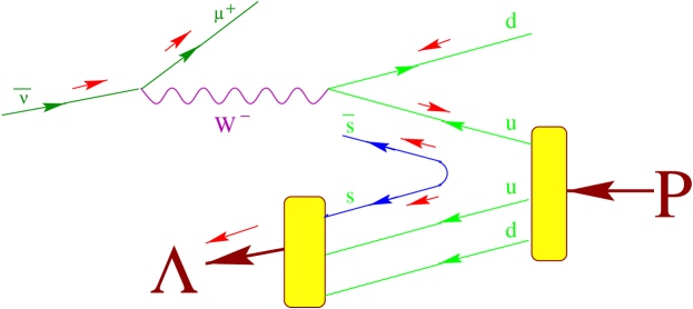
Figure 31: Dominant diagram for $\Lambda$ production in the target fragmentation region due to the scattering on a valence $u$-quark. Each small arrow represents the longitudinal polarization of the corresponding particle.

In the quark–parton model of deep inelastic $\nu$ or $\bar{\nu}$ scattering, the net longitudinal polarization $P_{s}$ of the remnant $s$ quark is given by

$$P_{s}={\sum_{q}C_{s\,q}N_{q}-\sum_{\bar{q}}C_{s\,\bar{q}}N_{\bar{q}}\over N_{q}+N_{\bar{q}}},$$ (107)

where $N_{q}$ ($N_{\bar{q}}$) is the total number of events in which a quark (antiquark) is struck, and $C_{s\,q}$ is the spin-correlation coefficient. The antiquarks contribute with a negative sign because their CC weak interactions are right-handed. The final $\Lambda$ polarization $P_{\Lambda}=D_{F}\,P_{s}$, where $D_{F}$ is a dilution factor that describes the spin transfer during hadronization.

Let us consider also the scenario ${\bf B}$, where both projections $L_{z}(\bar{s}s)=+1$ and $L_{z}(\bar{s}s)=0$ of the $\bar{s}s$-pair angular momentum contribute with equal probabilities. $L_{z}(\bar{s}s)=0$ means neglecting the transverse motion of the $\bar{s}s$ pair  [178].

The correlation of the remnant $s$-quark polarization with that of any other struck sea quark ($q_{sea}\neq\bar{s}$) depends on whether they come from the same parent constituent quark. If they do, which might be the dominant case, then a strong spin-correlation is expected (case a). Otherwise, the correlation should be reduced (case b). Then for the spin-correlation coefficients we have

$${\bf A:}\quad C_{sq_{val}} =-1,\;C_{s\bar{s}}=1$$

$${\bf B:}\quad C_{sq_{val}} =-{1\over 3},\;C_{s\bar{s}}={1\over 3}$$

$${\bf Aa:}\quad C_{sq_{sea}} =1,$$ (108)

$${\bf Ba:}\quad C_{sq_{sea}} ={1\over 9},$$

$${\bf Ab,Bb:}C_{sq_{sea}} =0.$$

The results for the remnant $s$-quark polarization and the predictions of NQM are presented in the Table 10 together with the measured $\Lambda$  polarization.

Table 10: $\Lambda$ polarization in the TFR of (anti)neutrino SIDIS. Model predictions in boldface lie within $\pm 1\sigma$ of the experimental data.

Experiment (Reaction)	Data	Aa	Ab	Ba	Bb	NQM
WA21 [155] ($\nu_{\mu}-p$)	-0.29 $\pm$ 0.18	-0.51	-0.75	-0.22	-0.25	-0.55
WA21 [155] ($\bar{\nu}_{\mu}-p$)	-0.38 $\pm$ 0.18	-0.85	-0.92	-0.30	-0.31	0.03
WA59 [156] ($\bar{\nu}_{\mu}-Ne$)	-0.63 $\pm$ 0.13	-0.82	-0.91	-0.29	-0.30	-0.30
E632 [157] ($\nu_{\mu}-Ne$)	-0.43 $\pm$ 0.20	-0.70	-0.84	-0.27	-0.27	-0.30
NOMAD [158] ($\nu_{\mu}-C$)	-0.21 $\pm$ 0.04	-0.59	-0.80	-0.24	-0.27	-0.30
NOMAD [158] ($\nu_{\mu}-``p^{\prime\prime}$)	-0.29 $\pm$ 0.06	-0.54	-0.77	-0.23	-0.26	-0.55
NOMAD [158] ($\nu_{\mu}-``n^{\prime\prime}$)	-0.16 $\pm$ 0.05	-0.61	-0.81	-0.25	-0.27	0.03

The data on longitudinal $\Lambda$ polarization from the NOMAD experiment [158] have the best statistical accuracy, and we will base the conclusions mainly on comparisons with these data. As one can see from Table 10:

• the predictions of NQM are not so different from the NOMAD data on the isoscalar (mainly carbon) target, but contradict the NOMAD $p$ and $n$ and the WA21 data;

• the meson-cloud model predicts zero polarization and is in contradiction with all data;

• the best description of the NOMAD data is achieved in the polarized-intrinsic-strangeness model with scenarios Ba and Bb, provided that $D_{F}\approx 1$. The remnant $s$-quark polarization is higher in absolute value for the Aa and Ab scenarios. If one allows a large depolarization during hadronization, $D_{F}\approx 0.4$-$0.5$, then the scenarios Aa and Ab can also provide a fair description of all data.

It is possible to distinguish between scenarios A and B of the last model by measuring the $\bar{\Lambda}$ polarization in the TFR of the neutrino SIDIS. One should expect that $P_{\bar{\Lambda}}\approx P_{\Lambda}$ in case A and $P_{\bar{\Lambda}}\approx 3P_{\Lambda}$ in case B.

The models predict different polarizations for intrinsic $s$- and $\bar{s}$-quark sea:

• NQM: $\Delta s=\Delta\bar{s}=0$;

• meson-cloud model [26]:$\Delta\bar{s}\approx 0,\,\Delta s<0$;

• intrinsic-strangeness-model A: $\Delta s\approx\Delta\bar{s}<0$;

• intrinsic-strangeness-model B: $\Delta s\approx 1/3;\;\Delta\bar{s}<0$;

In principle, these predictions can be independently tested by measuring the asymmetries of strange-particle production in the current fragmentation region of SIDIS or of (anti)neutrino DIS on a polarized target.

One could try to improve the naive quark model by taking into account the $SU(6)$ symmetry breaking as it was done in [168]. In the meson-cloud model one can expect that the contributions from higher possible fluctuations with vector meson $K^{+*}\Lambda$ will lead to non-zero $\Lambda$ polarization. However, the estimates of ref. [26] show that the relative probability of this state is small with respect to $K^{+}\Lambda$ (less than 10%). Moreover they predict a positively-correlated $s$-quark spin in a polarized proton.

9.3 Discussion

The study of $\Lambda$ polarization in the CFR allows us to understand the spin transfer from the quarks to the $\Lambda$. Due to the natural helicity and flavour selection of neutrino couplings, we can precisely single out specific quark contributions: this information cannot be obtained from the usual lepton-initiated DIS. The information on polarized and unpolarized fragmentation functions into $\Lambda$ which is available from LEP data is scarce and uncertain; also data from NOMAD are far from being decisive in fixing the features of quark-spin transfer. The $\nu$-Factory  data will induce a big improvement in our understanding of fragmentation processes.

In the target fragmentation region, one can study a new phenomenon, namely, the polarization transfer from the lepton to the final hadron. The models discussed here are the first attempts to describe this effect. The different models of spin transfer from a polarized quark to a polarized $\Lambda$ are able to describe the existing LEP data but give different predictions for (anti)neutrino DIS (see, for example, [164, 170] and [179] where comparison with NOMAD data are presented).

Finally, we would like to mention that the best existing data on $\Lambda$ polarization, which come from the NOMAD experiment, are based on the analysis of about one million DIS events. The statistics at the $\nu$-Factory is expected to be a hundred times higher, thus providing ten times better statistical accuracy. This will provide a more detailed study of the $\Lambda$ polarization dependence on kinematic variables and allow better comparisons with different model predictions.

10 SEARCHES FOR NEW PHYSICS

We now review briefly some prospects in searching for new physics using the intense beams from a neutrino factory.

10.1 A search for $\mathbf{Z}^{\prime}$ in muon–neutrino-associated charm production

In many extensions of the SM the presence of an extra neutral boson, $Z^{\prime}$, is invoked. A precision study of weak NC-exchange processes involving only second-generation fermions is still missing. A search for $Z^{\prime}$ in muon–neutrino-associated charm production has recently been proposed [180]. This process only involves $Z^{\prime}$ couplings with fermions from the second generation. It is interesting because an exotic $Z^{\prime}$ with stronger coupling to the $I_{3}=1/2$ component of weak isospin doublets could still give measurable effects at neutrino factories, unlike LHC experiments, which are only sensitive to the $Z^{\prime}$ coupling to charged leptons ($I_{3}=-1/2$).

We briefly review the method and the application to neutrino factories using an ideal detector. For a detailed discussion of this method, see Ref. [180].

10.1.1 The process

At $Q^{2}\ll M_{Z}^{2}$ the NC effective Lagrangian ruling the associated charm production induced by $\nu_{\mu}$ and including the new physics term is given by [180]

$${\cal L}_{T}^{\nu c\overline{c}}=-{G_{F}\over\sqrt{2}}\overline{\nu}_{\mu}\gamma^{\alpha}(1-\gamma_{5})\nu_{\mu}~{}\overline{c}\gamma_{\alpha}\left[\epsilon_{V}(c)-\epsilon_{A}(c)\gamma_{5}\right]c~{}~{}~{},$$ (109)

where

$$\epsilon_{V}(c) = \epsilon_{L}(u)+\epsilon_{R}(u)+\left(M_{Z}^{2}\over M_{Z^{\prime}}^{2}\right)(\eta_{L}+\eta_{R})$$ (110)

$$\equiv \epsilon_{V}(u)+\left(M_{Z}^{2}\over M_{Z^{\prime}}^{2}\right)\eta_{V}=\left[1+\left(M_{Z}^{2}\over M_{Z^{\prime}}^{2}\right)x\right]\epsilon_{V}(u)~{}~{}~{},$$

$$\epsilon_{A}(c) = \epsilon_{L}(u)-\epsilon_{R}(u)+\left(M_{Z}^{2}\over M_{Z^{\prime}}^{2}\right)(\eta_{L}-\eta_{R})$$ (111)

$$\equiv \epsilon_{A}(u)+\left(M_{Z}^{2}\over M_{Z^{\prime}}^{2}\right)\eta_{A}=\left[1+\left(M_{Z}^{2}\over M_{Z^{\prime}}^{2}\right)y\right]\epsilon_{A}(u)~{}~{}~{},$$

and the parameters $x$ and $y$ give the departure of the couplings from SM predictions.

10.1.2 Description of the method

The peculiar topology of the associated charm production in $\nu_{\mu}$ NC interactions is exploited: two charmed hadrons in the final state. Consequently, there are no other physical processes that may mimic it. Experimentally we are sensitive to the ratio

$$R={\sigma_{c\bar{c}}^{NC}\over\sigma^{CC}}$$ (112)

which can be written as the product

$$R={\sigma_{c\bar{c}}^{NC}(Z^{0}+Z^{\prime})\over\sigma_{c\bar{c}}^{NC}(Z^{0})}\times{\sigma_{c\bar{c}}^{NC}(Z^{0})\over\sigma^{CC}}=r\times f$$ (113)

where $\sigma_{c\bar{c}}^{NC}(Z^{0})$ is the cross section of the associated charm-production process in $\nu_{\mu}$ interactions in the absence of the $Z^{\prime}$ boson, $\sigma_{c\bar{c}}^{NC}(Z^{0}+Z^{\prime})$ includes the contribution of the new neutral boson, and $\sigma^{CC}$ is the $\nu_{\mu}$ DIS CC cross section.

From Eq. (113) it is clear that the relevant information about the $Z^{\prime}$ comes from the ratio $r$, which is unity in absence of the $Z^{\prime}$. In the following we assume a $50$ GeV mono-energetic $\nu_{\mu}$ beam . Under this assumption, by using the HERWIG simulation program to compute the the ratio $f$, we get $f=(1.25\pm 0.01)\times 10^{-4}$.

If we parameterize the ratio $r$ in terms of the $x$, $y$ and $M^{2}_{Z^{\prime}}$ variables defined in Section 10.1.1, the most general expression we obtain is:

$$r(x,y,M^{2}_{Z^{\prime}})=1+\left(500\over M_{Z^{\prime}}\right)^{2}(A_{1}y+B_{1}x)+\left(500\over M_{Z^{\prime}}\right)^{4}(A_{2}y^{2}+B_{2}x^{2}+C_{1}xy).$$ (114)

Fitting the data from the calculation with the previous function, we obtain the following values of the coefficients: $A_{1}=0.1$, $A_{2}=0.003$, $B_{1}=0.02$, $B_{2}=0.0007$ and $C_{1}=-0.0002$. The fit is valid in the $[-30,30]$ range for both $x$ and $y$ variables. Figure 32 shows the fitted function $r$ for $M_{Z^{\prime}}=500~{}\mbox{GeV/c}^{2}$.

Figure 32: The ratio $r$ is plotted by assuming $M_{Z^{\prime}}=500~{}{\mathrm{G}eV}/c^{2}$.

The number of observed events, $N_{S}$, can be written as

$$N_{S}=N_{c\bar{c}}\cdot{\varepsilon_{S}\over\varepsilon_{B}}\cdot r\;,$$ (115)

where $N_{c\bar{c}}$ is the number of observed events without the $Z^{\prime}$ effect, $\varepsilon_{S}$ and $\varepsilon_{B}$ are the reconstruction efficiencies for the events with and without a $Z^{\prime}$, respectively.

10.1.3 Measurement accuracy

Once the charmed particles have been tagged, the $Z^{\prime}$ effect would show up as an excess/defect of doubly charmed events in NC interactions. From Eq. (114) we can argue that for ‘large’ $Z^{\prime}$ couplings, i.e. $x$ and $y>20$, we can get an enhancement of the associated charm production of about a factor 7. On the other hand, if we do not observe any excess/defect, we can put a limit on the $x$ and $y$ parameters. As an example we report in Fig. 33 the sensitivity plot at 95% C.L. for the $x$ and $y$ variables at $M_{Z^{\prime}}$ = 500 GeV$/c^{2}$. Different systematic errors are assumed from 1% to 50%.

The allowed region of parameters is obtained from the formula

$$1-1.96\cdot{\sigma\over N_{c\bar{c}}}\leq{\varepsilon_{S}\over\varepsilon_{B}}\cdot r\leq 1+1.96\cdot{\sigma\over N_{c\bar{c}}}\;,$$ (116)

where $\sigma$ is defined as

$$\sigma=(\varepsilon^{2}_{stat}+\varepsilon^{2}_{syst})$$ (117)

and includes the error on the event counting from both a statistical and systematics sources. The factor 1.96 takes into account the required confidence level.

In Fig. 33, for each plot, the two lines bound the region of coupling parameters where no significant excess/defect of associated charm-production events is found. In other words, an observation of a number of charm pair events in agreement with SM predictions excludes the regions outside the band. For each plot shown in Fig. 33, we report in Table 11 the $\Delta x$ and $\Delta y$ values, respectively the bandwidth at $y=-30$ and $x=-30$.

Scenario	Present experiments		$\nu$-Factory
$\varepsilon$	$\Delta x$	$\Delta y$	$\Delta x$	$\Delta y$
0.01	12.0	5.5	2.5	1.5
0.10	12.5	6.0	3.5	2.0
0.25	14.0	6.5	6.5	3.0
0.50	18.0	8.0	13.0	5.5

Table 11: Band widths at $x=-30$ and $y=-30$ for all the sensitivity plots shown in Fig. 33. $\varepsilon$ indicates the systematic uncertainty.

We assume that $10^{7}$ CC interactions are collected at the $\nu$-Factory. Figure 33 shows the comparison between the sensitivity achievable with present experiments (say CHORUS) and the one obtainable at a $\nu$-Factory. At a $\nu$-Factory  the systematic uncertainties would play an important role if they are larger than about 10%, while the statistics is the leading contribution for present experiments.

Figure 33: The sensitivity plots for the $x$ and $y$ variables at $M_{Z^{\prime}}$ = 500 GeV$/c^{2}$ are shown. $\varepsilon$ indicates the systematic error. $10^{7}$ CC interactions are assumed to be collected at a $\nu$-Factory  (right plot). The sensitivity achievable with present experiments is also considered (left plot).

10.2 Bounds on 4-fermion operators from a $\mathbf{\nu}$-Factory

Many types of Beyond-the-Standard-Model (BSM) physics appear at energy scales above that of the neutrino-scattering process, so their tree-level effects at a $\nu$-Factory  can be parametrized by 4-fermion operators. These can contribute in the $\mu^{\pm}$ decay, or in the scattering in the detector. All new physics induced by scalars or vectors can be written, via Fierz transformations, as $(V\pm A)(V-A)$ vertices, which we normalize as:

$$\eta_{PL}^{\bar{\ell}e\bar{\nu}\nu}(\bar{\ell}\gamma^{\alpha}Pe)(\bar{\nu}\gamma_{\alpha}P_{L}\nu),~{}~{}~{}~{}\eta_{PL}^{\bar{u}_{i}d_{j}\bar{\ell}\nu}(\bar{u}_{i}\gamma^{\alpha}Pd_{j})(\bar{\ell}\gamma_{\alpha}P_{L}\nu)\;,$$ (118)

where $P=P_{L}=(1-\gamma_{5})/2$ or $P=P_{R}=(1+\gamma_{5})/2$, and $\ell$ is a charged lepton. Neutrinos without index can be of any flavour. We assume that the strongest neutrino interactions are SM weak, so that the neutrino-flavour basis makes sense perturbatively (see ref. [182]).

Bounds on a variety of extensions of the SM from neutrino scattering were reviewed in [183]; a brief update can be found in [142]. New physics in neutrino scattering that cannot be parametrized by 4-fermion operators has recently been discussed in [3]. A catalogue of old constraints on 4-fermion operators can be found in Refs. [183] (many models) and [184] (leptoquarks and bileptons)—more up-to-date bounds are reviewed in [185] ($Z^{\prime}$s) and many other recent papers. Constraints on $Z^{\prime}$s from a neutrino factory were studied in the previous section, and bounds on $R$-parity-violating couplings from neutrino scattering have been discussed in [186].

A $\nu$-Factory can improve bounds on 4-fermion operators involving neutrinos by many orders of magnitude. However, since neutrinos are weakly interacting, the resulting bounds are generically weaker than bounds on 4-fermion operators involving charged leptons rather than neutrinos. For instance, new physics that can contribute both to lepton-flavour violation in neutrino scattering and to $\mu\rightarrow e\gamma$ will be more strongly constrained (or more readily detected) in $\mu\rightarrow e\gamma$ than in neutrino scattering, as can be seen from the bounds on lepton-flavour violation discussed in the Report of the Stopped-Muon Working Group [187]. It could nonetheless be interesting to look for BSM physics in neutrino scattering at the near detector of a neutrino factory.

First of all, any observed lepton-flavour violation must be due to something other than oscillations. Neutrinos are in fact produced only a few hundred metres away from the detector, and have no time to oscillate, given the current determinations of the mixing parameters. New physics that can be parametrized by 4-fermion operators can then be distinguished from oscillations.

Secondly, there is BSM physics that can induce $\nu\nu\ell\ell$ 4-fermion operators, without inducing $\ell\ell\ell\ell$ operators ($\ell$ is a charged lepton.) For quarks, BSM physics (e.g.  LQ, $Z^{\prime}$) that induces $\nu\bar{\nu}qq$ also induces $\ell\bar{\ell}qq$, so we do not discuss operators involving quarks. There could nonetheless be interesting limits on flavour-changing vertices involving charm quarks, from neutrino scattering off nucleons, because rare $D$-meson decays are poorly measured.

As explained above, we only consider the case of flavour violation induced in the muon decay. Since we do not carry out a complete simulation of the event rates, we shall assume that the kinematics of the muon decay induced by the first vertex in Eq. (118) is the same as for the SM $(V-A)(V-A)$ current. We shall then parameterize the muon-decay rate induced by the vertex (118) as:

$$\Gamma(\mu\rightarrow e\bar{\nu}_{i}\nu_{j})=\left({\eta_{PL}^{\bar{\mu}e\bar{\nu}_{i}\nu_{j}}\over 2\sqrt{2}G_{F}}\right)^{2}\Gamma_{SM}(\mu\rightarrow e\bar{\nu}_{e}\nu_{\mu})\equiv[\epsilon_{PL}^{\bar{\mu}e\bar{\nu}_{i}\nu_{j}}]^{2}\Gamma_{SM}(\mu\rightarrow e\bar{\nu}_{e}\nu_{\mu})$$ (119)

and will assume the neutrino beam shapes induced by these BSM decays to be approximated by the SM one.

The new physics signal that we explore is given by a final-state $\tau$ or by a wrong-sign muon (WSM; e.g.  a $\mu^{+}$ produced in the detector by a neutrino beam produced in $\mu^{-}$ decay). These signals do not suffer from any irreducible physics background. Some $\tau$’s can be produced in the decays of charmed mesons produced by SM CC interactions, but in principle these events will also contain an electron or muon from the CC vertex. The $\tau$ decays from charm produced in NC neutrino interactions, can be vetoed by identifying the second charm in the event. Similar considerations apply to events with WSMs. As a consequence, a meaningful estimate of the background rates is not possible without a concrete detector study. To quantify the discovery potential, we therefore limit ourselves to presenting a sensitivity reach for the detection of $N$ anomalous events, assuming 100% reconstruction efficiency for the BSM signal. We assume $10^{6}~{}\nu e$ and $10^{8}~{}\nu N$ scattering interactions per year in the detector due to SM CC interactions. Then BSM physics could be detected in $\nu e$ scattering if:

$${\eta\over 2\sqrt{2}G_{F}}\equiv\epsilon>\sqrt{N}\times 10^{-3}$$ (120)

and could be detected in $\nu N$ scattering if:

$${\eta\over 2\sqrt{2}G_{F}}\equiv\epsilon>\sqrt{N}\times 10^{-4}$$ (121)

Notice that while the reach is lower with $\nu e$ scattering, the detector backgrounds could be much smaller, and any future detailed study will have to consider the possibility offered by this channel. The results we present here are obtained assuming the event rates from $\nu N$ scattering.

We list in Table 12 the lepton-flavour-violating 4-fermion operators on which a $\nu$ factory could set better bounds than are available now. In the first column, we list $\bar{\mu}e\bar{\nu}\nu$ vertices of different chirality. This is a useful way of listing 4-fermion vertices because the new physics that generates them could depend on fermion chirality. In the second column are the best available limits yet on the operators, and the processes from which the bounds come. In the last column are the limits that a $\nu$-Factory  could set, assuming a 10 event sensitivity ($N=10$ in Eqs. 120 and 121). Horizontal lines in the last column separate operators that are distinguishable at a $\nu$-Factory because they induce different final-state particles in the detector; polarized muons would be required to distinguish between LL and RL couplings. Similarly, horizontal lines in the second column separate operators that are distinguishable in present experiments (where the flavour of the outgoing neutrinos is often not detected).

Table 12: Flavour changing four fermion vertices involving neutrinos, which a $\nu$ factory could set a bound on. Neutrinos with index $i$ can be of any flavour. The processes listed in parenthesis presently constrain (at 90 % cl) the coefficients of the four fermion vertices to be less than $\epsilon\times 2\sqrt{2}G_{F}$. A neutrino factory could set bounds given in the last column. These bounds assume that all 4-fermion operators other than the contrained one are absent. Note that there are much stronger bounds on $\bar{\ell}_{i}\ell_{j}\bar{\ell}_{k}\ell_{l}$ vertices than the quoted bounds on $\bar{\ell}_{i}\ell_{j}\bar{\nu}_{k}\nu_{l}$.

Vertex	Current limits	$\nu$-Factory limit
$(\bar{\mu}\gamma^{\alpha}P_{L}{e})(\bar{\nu}_{\tau}\gamma_{\alpha}P_{L}\nu_{i})$	$|\epsilon|<0.06$ ($\nu$ oscillations)	$3\times 10^{-4}$
$(\bar{\mu}\gamma^{\alpha}P_{R}{e})(\bar{\nu}_{\tau}\gamma_{\alpha}P_{L}\nu_{i})$	$|\epsilon|<0.03$ ($G_{\mu}(g^{S}_{RR})$)	$3\times 10^{-4}$
$(\bar{\mu}\gamma^{\alpha}P_{L}{e})(\bar{\nu}_{\mu}\gamma_{\alpha}P_{L}\nu_{i})$	$|\epsilon|<0.1$ ($\mu\rightarrow e{\nu}_{e}\bar{\nu}_{\mu}$)	$3\times 10^{-4}$
$(\bar{\mu}\gamma^{\alpha}P_{R}{e})(\bar{\nu}_{\mu}\gamma_{\alpha}P_{L}\nu_{i})$	$|\epsilon|<0.03$ ($G_{\mu}(g^{S}_{RR})$)	$3\times 10^{-4}$
$(\bar{\mu}\gamma^{\alpha}P_{R}{e})(\bar{\nu}_{i}\gamma_{\alpha}P_{L}\nu_{\tau})$	$|\epsilon|<0.03$ ($G_{\mu}(g^{S}_{RR})$)	$3\times 10^{-4}$
$(\bar{\mu}\gamma^{\alpha}P_{L}{e})(\bar{\nu}_{i}\gamma_{\alpha}P_{L}\nu_{\tau})$	$|\epsilon|<0.2$ ($G_{\mu}$)	$3\times 10^{-4}$

11 CONCLUSIONS

This work documents our assessment of the physics potential of detectors placed at the front-end of a high-current muon storage ring. In most of the cases presented, we tried to evaluate in quantitative terms the ultimate accuracies that can be reached, given the available statistics and given the theoretical knowledge available today.

In the case of determinations of the partonic densities of the nucleon, we proved that the $\nu$-Factory could significantly improve the already good knowledge we have today. In the unpolarized case, the knowledge of the valence distributions would improve by more than one order of magnitude, in the kinematical region $x\mathrel{\vbox{\hbox{$>$}\nointerlineskip\hbox{$\sim$}}}0.1$, which is best accessible with 50 GeV muon beams. The individual components of the sea ($\bar{u}$, $\bar{d}$, ${s}$ and $\bar{s}$), as well as the gluon, would be measured with relative accuracies in the range of 1–10%, for $0.1\mathrel{\vbox{\hbox{$<$}\nointerlineskip\hbox{$\sim$}}}x\mathrel{\vbox{\hbox{$<$}\nointerlineskip\hbox{$\sim$}}}0.6$. The high statistics available over a large range of $Q^{2}$ would furthermore allow the accurate determination of higher-twist corrections, strongly reducing the theoretical systematics that affect the extraction of $\alpha_{\scriptscriptstyle\mathrm{S}}$ from sum rules and global fits.

In the case of polarized densities, we stressed the uniqueness of the $\nu$-Factory as a means of disentangling quark and antiquark distributions, and their first moments in particular. These can be determined at the level of few per cent for up and down, and 10% for the strange, sufficient to distinguish between theoretical scenarios, and thus allowing a full understanding of the proton spin structure. A potential ability to pin down the shapes of individual flavour components with accuracies at the level of few per cent is limited by the mixing with the polarized gluon. To identify this possible weakness of the $\nu$-Factory polarized-target programme, it was crucial to perform our analysis at the NLO; we showed in fact that any study based on the LO formalism would have resulted in far too optimistic conclusions. This holds true both in the case of determinations based on global fits and on direct extractions using flavour tagging in the final state. Our conclusion here is that a full exploitation of the $\nu$-Factory potential for polarized measurements of the shapes of individual partonic densities requires an a-priori knowledge of the polarized gluon density. It is hoped that the new information expected to arise from the forthcoming set of polarized DIS experiments at CERN, DESY and RHIC will suffice.

The situation is also very bright for measurements of C–even distributions. Here, the first moments of singlet, triplet and octet axial charges can be measured with accuracies which are up to one order of magnitude better than the current uncertainties. In particular, the improvement in the determination of the singlet axial charge would allow a definitive confirmation or refutation of the anomaly scenario compared to the ‘instanton’ or ‘skyrmion’ scenarios, at least if the theoretical uncertainty originating from the small–$x$ extrapolation can be kept under control. The measurement of the octet axial charge with a few percent uncertainty will allow a determination of the strange contribution to the proton spin better than 10%, and allow stringent tests of models of $SU(3)$ violation when compared to the direct determination from hyperon decays.

The measurement of two fundamental constants of nature, $\alpha_{\scriptscriptstyle\mathrm{S}}(M_{Z})$ and $\sin^{2}\theta_{W}$, will be possible using a variety of techniques. At best the accuracy of these measurements will match or slightly improve the accuracy available today, although the measurements at the $\nu$-Factory are subject to different systematics and therefore provide an important consistency check of current data. In the case of $\alpha_{\scriptscriptstyle\mathrm{S}}(M_{Z})$, the dependence of the results on the modeling of higher-twist corrections both in the structure function fits and in the GLS sum rule is significantly reduced relative to current measurements, as mentioned above. In the case of $\sin^{2}\theta_{W}$, its determination via $\nu e$ scattering at the $\nu$-Factory has an uncertainty of approximately $2\times 10^{-4}$, dominated by the statistics and the luminosity measurement. This error is comparable to what already known today from EW measurements in $Z^{0}$ decays. Compared to these, however, this determination would improve current low-energy extractions, and be subject to totally different systematic uncertainties. It would also be sensitive to different classes of new-physics contributions. The extrapolation to $Q=M_{Z}$ is affected, at the same level of uncertainty, by the theoretical assumptions used in the evaluation of the hadronic-loop corrections to $\gamma$-$Z$ mixing. The determination via DIS, on the other hand, is limited by the uncertainties on the heavy-flavour parton densities. As shown earlier, these should be significantly reduced using the $\nu$-Factory data themselves.

In several other areas, the data from the $\nu$-Factory will allow quantitative studies to be made of phenomena that, so far have only been explored at a mostly qualitative level. This is the case of the exclusive production of charmed mesons and baryons (leading to very large samples, suitable for precise extractions of branching ratios and decay constants), of the study of spin-transfer phenomena, and of the study of nuclear effects in DIS. While nuclear effects could be bypassed at the $\nu$-Factory by using hydrogen targets directly, the flavour separation of partonic densities will require using also targets containing neutrons. This calls for an accurate understanding of nuclear effects. The ability to run with both $H$ and heavier targets will in turn provide rich data sets useful for quantitative studies of nuclear models. The study of $\Lambda$ polarization both in the target and in the fragmentation regions, will help clarifying the intriguing problem of spin transfer. We reviewed several of the existing models, and indicated how semi-inclusive neutrino DIS will allow the identification of the right ones, as well as providing input for the measurement of polarized fragmentation functions.

Finally, we presented some cases of exploration for physics beyond the SM using the $\nu$-Factory data. Although the neutrino beam energies considered in our work are well below any reasonable threshold for new physics, the large statistics makes it possible to search for manifestations of virtual effects. The exchange of new gauge bosons decoupled from the first generation of quarks and leptons can be seen via enhancements of the inclusive charm production rate, with a sensitivity well beyond the present limits. Rare lepton-flavour-violating decays of muons in the ring could be tagged in the DIS final states through the detection of wrong-sign electrons and muons, or of prompt taus. Once again, the sensitivity at the $\nu$-Factory goes well beyond existing limits.

The work presented here has two clear weaknesses, which point to two directions for further work. On one side, a realistic evaluation of the experimental feasibility of the proposed measurements should be performed. Concrete detector designs should be proposed, and the detector performance should be evaluated in the light of the statistical and theoretical accuracy reach set by our study. As part of this work, an optimization of the beam parameters (energy, length of the straight section, distance of the detector from the ring) should be performed for each individual physics task. On the other side, we made no any effort to present a physics case justifying a set of goals for the performances. Considering that these results will not be available before at least 10–15 years from now, some judgement on the merit of these measurements has to be given. For example, why should we want to know 15 years from now the strange density of the proton with an accuracy of 1%? How would our knowledge of fundamental physics, or our ability to predict new phenomena, improve if we could reach this goal? From the measurements listed in this document, which ones will be the most important at the time when the $\nu$-Factory will be operating? We hope that future studies of this new and fascinating facility will address this important aspect of the case for front-end experiments.

References

- [1] S. Geer, Phys. Rev. D57 (1998) 6989 [hep-ph/9712290], [Erratum-ibid. D59 (1999) 039903.]
-
[2]
The Muon Collider Collab., Collider: a feasibility study,
Report BNL-52503, Fermilab-Conf-96/092, LBNL-38946 (1996);
B. Autin, A. Blondel and J. Ellis (eds.), Prospective study of muon storage rings at CERN, Report CERN 99-02, ECFA 99-197 (Geneva, 1999). - [3] I. Bigi et al., The potential for neutrino physics at muon colliders and dedicated high current muon storage rings, Report BNL-67404.
- [4] C. Albright et al., hep-ex/0008064.
- [5] R.D. Ball, D.A. Harris and K.S. McFarland, hep-ph/0009223, submitted to the Proceedings of the Nufact ’00 Workshop, June 2000, Monterey.
- [6] H.L. Lai et al., Phys. Rev. D55 (1997) 1280 [hep-ph/9606399].
- [7] V. Barone, C. Pascaud and F. Zomer, Eur. Phys. J. C12 (2000) 243 [hep-ph/9907512].
- [8] S. I. Alekhin, Phys. Rev. D 63 (2001) 094022 [hep-ph/0011002].
-
[9]
G. Ridolfi, Nucl. Phys. A666 (2000) 278;
R.D. Ball and H.A.M. Tallini, Jour. Phys. G25 (1999) 1327;
S. Forte, hep-ph/9409416 and hep-ph/9610238. - [10] S. Forte, M.L. Mangano and G. Ridolfi, hep-ph/0101192, to appear in Nucl. Phys. B.
- [11] J. Blümlein and N. Kochelev, Phys. Lett. B381 (1996) 296 and Nucl. Phys. B498 (1997) 285.
- [12] D.A. Dicus, Phys. Rev. D5 (1972) 1637.
-
[13]
M. Anselmino, P. Gambino and J. Kalinowski, Z. Phys. C64 (1994) 267;
M. Maul et al., Z. Phys. A356 (1997) 443;
J. Blümlein and N. Kochelev, Nucl. Phys. B498 (1997) 285;
V. Ravishankar, Nucl. Phys. B374 (1992) 309. -
[14]
B. Ehrnsperger and A. Schäfer, Phys. Lett. B348 (1995) 619;
J. Lichtenstadt and H.J. Lipkin, Phys. Lett. B353 (1995) 119;
J. Dai et al., Phys. Rev. D53 (1996) 273;
P.G. Ratcliffe, Phys. Lett. B365 (1996) 383;
N.W. Park, J. Schechter and H. Weigel, Phys. Lett. B228 (1989) 420. - [15] A.O. Bazarko et al., Z. Phys. C65 (1989) 189.
-
[16]
R. Mertig and W.L. van Neerven, Z. Phys. C70 (1996) 637;
W. Vogelsang, Phys. Rev. D54 (1996) 2023. - [17] D. de Florian and R. Sassot, Phys. Rev. D51 (1995) 6052.
- [18] R.D. Ball, S. Forte and G. Ridolfi, Phys. Lett. B378 (1996) 255.
- [19] G. Altarelli, S. Forte and G. Ridolfi, Nucl. Phys. B534 (1998) 277 and Nucl. Phys. B (Proc. Suppl.) 74 (1999) 138.
- [20] G. Altarelli, R.D. Ball, S. Forte and G. Ridolfi, Acta Phys. Polon. B29 (1998) 1145 [hep-ph/9803237].
- [21] H.L. Lai et al. (CTEQ Collab.), Eur. Phys. J. C12 (2000) 375 [hep-ph/9903282].
- [22] G. Altarelli, R.D. Ball, S. Forte and G. Ridolfi, Nucl. Phys. B496 (1997) 337 and Acta Phys. Polon. B29 (1998) 1145.
-
[23]
G. Altarelli and G.G. Ross, Phys. Lett. B212 (1988) 391;
A. V. Efremov and O. V. Teryaev, JINR-E2-88-287, in Proceedings of Symposium on Hadron Interactions-Theory and Phenomenology, Bechyne, June 26- July 1, 1988; ed. by J. Fischer et al (Czech. Acad. Sci., Inst. Phys., 1988) p.432;
R.D. Carlitz, J.C. Collins and A.H. Mueller, Phys. Lett. B214 (1988) 229;
G. Altarelli and B. Lampe, Z. Phys. C47 (1990) 315;
W. Vogelsang, Z. Phys. C50 (1991) 275. -
[24]
G.M. Shore and G. Veneziano, Phys. Lett. B244 (1990) 75 and Nucl. Phys. B381 (1992) 23;
see also G. M. Shore, hep-ph/9812355. -
[25]
S. Forte, Phys. Lett. B224 (1989) 189 and Nucl. Phys. B331 (1990) 1;
S. Forte and E.V. Shuryak, Nucl. Phys. B357 (1991) 153. - [26] S.J. Brodsky and B.-Q. Ma, Phys. Lett. B381 (1996) 317.
-
[27]
S.J. Brodsky, J. Ellis and M. Karliner, Phys. Lett. B206 (1988) 309;
J. Ellis and M. Karliner, hep-ph/9601280. - [28] M. Glück et al., hep-ph/0011215.
- [29] D. Adams et al. (Spin Muon Collab.), Nucl. Instrum. Meth. A437 (1999) 23.
-
[30]
B. Adeva et al. (SMC Collab.), Phys. Rev. D58 (1998) 112001;
P. L. Anthony et al. (E155 Collab.), Phys. Lett. B493 (2000) 19. - [31] R.M. Barnett, Phys. Rev. Lett. 36 (1976) 1163.
- [32] M.A. Aivazis, J.C. Collins, F.I. Olness and W. Tung, Phys. Rev. D 50 (1994) 3102.
- [33] T. Gehrmann and W.J. Stirling, Phys. Rev. D 53 (1996) 6100.
- [34] M. Glück, E. Reya, M. Stratmann and W. Vogelsang, Phys. Rev. D 53 (1996) 4775.
- [35] D.J. Gross and C.H. Llewellyn Smith, Nucl. Phys. B14 (1969) 337.
- [36] R. D. Ball and S. Forte, Phys. Lett. B358 (1995) 365 [hep-ph/9506233] and hep-ph/9607289.
- [37] J. Santiago and F.J. Yndurain, Nucl. Phys. B563 (1999) 45 [hep-ph/9904344].
-
[38]
V.S. Fadin and L.N. Lipatov, Phys. Lett. B429 (1998) 127;
M. Ciafaloni, D. Colferai and G. Salam, Phys. Rev. D60 (1999) 114036;
G. Altarelli, R.D. Ball and S. Forte, hep-ph/0011270. - [39] W.G. Seligman et al., Phys. Rev. Lett. 79 (1997) 1213.
- [40] A. L. Kataev, G. Parente and A.V. Sidorov, Nucl. Phys. B573 (2000) 405 [hep-ph/9905310].
- [41] A.L. Kataev, G. Parente and A.V. Sidorov, preprint CERN-TH/2000-343 [hep-ph/0012014], and work in progress.
- [42] S.I. Alekhin and A.L. Kataev, Phys. Lett. B452, 402 (1999) [hep-ph/9812348].
- [43] S. Bethke, J. Phys.G26 (2000) R27 [hep-ex/0004021].
- [44] I. Hinchliffe and A.V. Manohar, Annu. Rev. Nucl. Part. Sci. 50 (2000) 643 [hep-ph/0004186].
- [45] H. Georgi and H.D. Politzer, Phys. Rev. D14 (1976) 1829.
- [46] E.B. Zijlstra and W.L. van Neerven, Phys. Lett. B297 (1992) 377.
- [47] W.L. van Neerven and A. Vogt, Nucl. Phys. B568 (2000) 263 [hep-ph/9907472] and hep-ph/0103123.
- [48] W.L. van Neerven and A. Vogt, Phys. Lett. B490 (2000) 111 [hep-ph/0007362].
- [49] S.A. Larin, T. van Ritbergen and J.A. Vermaseren, Nucl. Phys. B427 (1994) 41.
- [50] S.A. Larin, P. Nogueira, T. van Ritbergen and J.A. Vermaseren, Nucl. Phys. B492 (1997) 338 [hep-ph/9605317].
- [51] A. Retey and J.A. Vermaseren, preprint TTP00-13, NIKHEF-2000-018, hep-ph/0007294.
- [52] J.A. Gracey, Phys. Lett. B322 (1994) 141 [hep-ph/9401214].
- [53] J. Blümlein and A. Vogt, Phys. Lett. B370 (1996) 149 [hep-ph/9510410].
- [54] S. Catani et al., preprint CERN-TH/2000-131 [hep-ph/0005025], in Standard model physics (and more) at the LHC, eds. G. Altarelli and M. Mangano, Report CERN 2000-004 (Geneva, 2000).
- [55] A.L. Kataev, A.V. Kotikov, G. Parente and A.V. Sidorov, Phys. Lett. B417 (1998) 374 [hep-ph/9706534].
- [56] M. Beneke, Phys. Rep. 317 (1999) 1 [hep-ph/9807443].
- [57] M. Beneke and V.M. Braun, hep-ph/0010208.
- [58] M. Dasgupta and B.R. Webber, Phys. Lett. B382 (1996) 273 [hep-ph/9604388].
- [59] M. Maul, E. Stein, A. Schafer and L. Mankiewicz, Phys. Lett. B401 (1997) 100 [hep-ph/9612300].
- [60] A.V. Sidorov et al. (IHEP–JINR Neutrino Detector Collab.), Eur. Phys. J. C10 (1999) 405 [hep-ex/9905038].
- [61] S.I. Alekhin et al. (IHEP-JINR Neutrino Detector Collab), preprint IHEP-01-18 (2001), [hep-ex/0104013].
- [62] C. Adloff et al. (H1 Collab.), hep-ex/0012052.
- [63] A.D. Martin, R.G. Roberts, W.J. Stirling and R.S. Thorne, Eur. Phys. J. C18 (2000) 117 [hep-ph/0007099].
- [64] E.B. Zijlstra and W.L. van Neerven, Nucl. Phys. B383 (1992) 525.
-
[65]
S.G. Gorishny and S.A. Larin, Phys. Lett. B172 (1986) 109;
S.A. Larin and J.A.M. Vermaseren, Phys. Lett. B259 (1991) 345. - [66] A.L. Kataev and A.V. Sidorov, preprint CERN-TH/7235-94 [hep-ph/9405254], in Proceedings of Rencontre de Moriond - Hadronic session of ‘QCD and high energy hadronic interactions’, Méribel-les-Allues, 1994, ed. J. Trân Thanh Vân (Editions Frontières, Gif-sur-Yvette, 1995), p. 189.
- [67] J.H. Kim et al., Phys. Rev. Lett. 81 (1998) 3595 [hep-ex/9808015].
- [68] J. Chyla and A.L. Kataev, Phys. Lett. B297 (1992) 385 [hep-ph/9209213].
- [69] A.L. Kataev and A.V. Sidorov, Phys. Lett. B331 (1994) 179 [hep-ph/9402342].
- [70] J. Blümlein and W. L. van Neerven, Phys. Lett. B450 (1999) 417 [hep-ph/9811351].
-
[71]
A.L. Kataev and V.V. Starshenko,
Mod. Phys. Lett. A10 (1995) 235 [hep-ph/9502348];
M.A. Samuel, J. Ellis and M. Karliner, Phys. Rev. Lett. 74 (1995) 4380 [hep-ph/9503411]. -
[72]
W. Bernreuther and W. Wetzel,
Nucl. Phys. B197 (1982) 228 [Erratum-ibid. B513 (1998)
758];
S.A. Larin, T. van Ritbergen and J.A. Vermaseren, Nucl. Phys. B438 (1995) 278 [hep-ph/9411260].
K.G. Chetyrkin, B.A. Kniehl and M. Steinhauser, Phys. Rev. Lett. 79 (1997) 2184 [hep-ph/9706430]. - [73] E.V. Shuryak and A.I. Vainshtein, Nucl. Phys. B199 (1982) 451.
- [74] M.A. Shifman, A.I. Vainshtein and V.I. Zakharov, Nucl. Phys. B147 (1979) 385.
- [75] V.M. Braun and A.V. Kolesnichenko, Nucl. Phys. B283 (1987) 723.
- [76] G.G. Ross and R.G. Roberts, Phys. Lett. B322 (1994) 425 [hep-ph/9312237].
- [77] J. Balla, M.V. Polyakov and C. Weiss, Nucl. Phys. B510 (1998) 327 [hep-ph/9707515].
-
[78]
R.G. Oldeman (CHORUS Collab.),
Nucl. Phys. Proc. Suppl. 79 (1999) 96;
R.G. Oldeman, PhD Thesis, Amsterdam University, June 2000 (unpublished). - [79] U.K. Yang et al. (CCFR–NuTeV Collab.), hep-ex/0010001.
- [80] J.D. Bjorken, Phys. Rev. 163 (1967) 1767.
-
[81]
W.A. Bardeen, A.J. Buras, D.W. Duke and T. Muta,
Phys. Rev. D18 (1978) 3998;
G. Altarelli, R.K. Ellis and G. Martinelli, Nucl. Phys. B143 (1978) 521. - [82] K.G. Chetyrkin, S.G. Gorishny, S.A. Larin and F.V. Tkachov, Phys. Lett. B137 (1984) 230.
- [83] S.A. Larin, F.V. Tkachov and J.A. Vermaseren, Phys. Rev. Lett. 66 (1991) 862.
- [84] M. Arneodo, Phys. Rep. 240 (1994) 301.
- [85] G. Piller and W. Weise, Phys. Rep. 330 (2000) 1 [hep-ph/9908230].
-
[86]
P. Amaudruz et al., Nucl. Phys. B441 (1995) 3;
M. Arneodo et al., Nucl. Phys. B441 (1995) 12. - [87] A.C. Benvenuti et al. (BCDMS Collab.), Phys. Lett. B189 (1987) 483.
- [88] J. Gomez et al., Phys. Rev. D49 (1994) 4348.
- [89] M.R. Adams et al. (E665 Collab.), Z. Phys. C67 (1995) 403 [hep-ex/9505006].
- [90] S.L. Adler, Phys. Rev. B135 (1964) 963.
- [91] J.S. Bell, Phys. Rev. Lett. 13 (1964) 57.
- [92] C.A. Piketti and L. Stodolsky, Nucl. Phys. B15 (1970) 571.
- [93] B.Z. Kopeliovich and P. Marage, Int. J. Mod. Phys. A8 (1993) 1513.
- [94] P.P. Allport et al. (BEBC WA59 Collab.), Phys. Lett. B232 (1989) 417.
- [95] C. Boros, J.T. Londergan and A.W. Thomas, Phys. Rev. D58 (1998) 114030 [hep-ph/9804410].
- [96] U.K. Yang et al. (CCFR–NuTeV Collab.), hep-ex/0009041.
-
[97]
M.A. Aivazis, F.I. Olness and W. Tung,
Phys. Rev. Lett. 65 (1990) 2339;
V. Barone, M. Genovese, N.N. Nikolaev, E. Predazzi and B. Zakharov, Phys. Lett. B268 (1991) 279 and Z. Phys. C70 (1996) 83 [hep-ph/9505343]. - [98] R.S. Thorne and R.G. Roberts, Phys. Lett. B421 (1998) 303 [hep-ph/9711223].
- [99] A.D. Martin, R.G. Roberts, W.J. Stirling and R.S. Thorne, Eur. Phys. J. C4 (1998) 463 [hep-ph/9803445].
- [100] L.L. Frankfurt, M.I. Strikman and S. Liuti, Phys. Rev. Lett. 65 (1990) 1725.
- [101] R. Kobayashi, S. Kumano and M. Miyama, Phys. Lett. B354 (1995) 465 [hep-ph/9501313].
- [102] K.J. Eskola, V.J. Kolhinen and P.V. Ruuskanen, Nucl. Phys. B535 (1998) 351 [hep-ph/9802350].
- [103] S.A. Kulagin, hep-ph/9812532.
- [104] P.V. Landshoff, J.C. Polkinghorne and R.D. Short, Nucl. Phys. B28 (1971) 225.
- [105] S.A. Kulagin, G. Piller and W. Weise, Phys. Rev. C50 (1994) 1154 [nucl-th/9402015].
- [106] S.V. Akulinichev, S.A. Kulagin and G.M. Vagradov, Phys. Lett. B158 (1985) 485.
- [107] S.A. Kulagin, Nucl. Phys. A500 (1989) 653.
- [108] G.B. West, Ann. Phys. NY 74 (1972) 464.
- [109] S.A. Kulagin and A.V. Sidorov, Eur. Phys. J. A9 (2000) 261 [hep-ph/0009150].
- [110] A.C. Benvenuti et al. (BCDMS Collab.), Z. Phys. C63 (1994) 29.
- [111] M. Vakili et al. (CCFR Collab.), Phys. Rev. D 61 (2000) 052003 [hep-ex/9905052].
- [112] S.A. Kulagin, Nucl. Phys. A640 (1998) 435 [nucl-th/9801039].
- [113] I.R. Afnan, F. Bissey, J. Gomez, A.T. Katramatou, W. Melnitchouk, G.G. Petratos and A.W. Thomas, nucl-th/0006003.
- [114] V. Guzey et al., hep-ph/0102133.
-
[115]
S. Sarantakos, A. Sirlin and W.J. Marciano,
Nucl. Phys. B217 (1983) 84;
D.Y. Bardin and V.A. Dokuchaeva, Sov. J. Nucl. Phys. 43 (1986) 975;
D.Y. Bardin and V.A. Dokuchaeva, Nucl. Phys. B287 (1987) 839. -
[116]
G. Degrassi et al. Phys. Lett. B350 (95) 75;
G. Degrassi and P. Gambino, Nucl. Phys. B567 (2000) 3. - [117] J.N. Bahcall, M. Kamionkowski and A. Sirlin, Phys. Rev. D51 (1995) 6146 [astro-ph/9502003].
- [118] See F. Jegerlehner, hep-ph/9901386 and references therein.
- [119] K.S. McFarland et al. (NuTeV Collab.), hep-ex/9806013, in Proceedings 33rd Rencontres de Moriond on Electroweak Interactions and Unified Theories, Les Arcs, 1998.
- [120] M. E. Peskin and T. Takeuchi, Phys. Rev. D 46 (1992) 381; W. J. Marciano and J. L. Rosner, Phys. Rev. Lett. 65 (1990) 2963 [Erratum-ibid. 68 (1990) 2963].
- [121] G. Altarelli and R. Barbieri, Phys. Lett. B 253 (1991) 161; D. C. Kennedy and P. Langacker, Phys. Rev. Lett. 65 (1990) 2967 [Erratum-ibid. 66 (1990) 2967].
- [122] D.E. Groom et al, Particle Data Group, Eur. Phys. J. 15 (2000) 1.
- [123] P. Migliozzi et al., Phys. Lett. B462 (1999) 217.
- [124] J. Finjord and F. Ravndal, Phys. Lett. B58 (1975) 61.
- [125] R.E. Shrock and B.W. Lee, Phys. Rev. D13 (1976) 2539.
- [126] C. Avilez et al., Phys. Lett. B66 (1977) 149.
- [127] C. Avilez and T. Kobayashi, Phys. Rev. D19 (1979) 3448.
- [128] C. Avilez et al., Phys. Rev. D17 (1978) 709.
- [129] A. Amer et al., Phys. Lett. B81 (1979) 48.
- [130] S.G. Kovalenko, Sov. J. Nucl. Phys. 52 (1990) 934.
- [131] G.T. Jones et al. (WA21 Collab.), Z. Phys. C36 (1987) 593.
- [132] V.V. Ammosov et al., JETP Lett. 58 (1993) 247.
- [133] D. Son et al., Phys. Rev. D28 (1983) 2129.
- [134] N. Ushida et al. (E531 Collab.), Phys. Lett. B206 (1988) 375.
- [135] N. Armenise et al., Phys. Lett. B104 (1981) 409.
- [136] G. De Lellis, P. Migliozzi and P. Zucchelli, Phys. Lett. B507 (2001) 7 [hep-ph/0104066]
- [137] G. Corcella et al., hep-ph/0011363.
- [138] T. Sjöstrand, report LU-TP-95-20, hep-ph/9508391.
- [139] G. Ingelman et al., Comput. Phys. Commun. 101 (1997) 108.
- [140] T. Bolton, hep-ex/9708014.
- [141] P. Annis et al. (CHORUS Collab.), Phys. Lett. B435 (1998) 458.
- [142] J. Conrad et al., Rev. Mod. Phys. 70 (1998) 1341.
- [143] T. Adams et al. (NuTeV Collab.), Phys. Rev. D61 (2000) 092001.
- [144] A.E. Asratian et al. (BBCN Collab.), Z. Phys. C58 (1993) 55.
- [145] J.D. Richman and P.R. Burchat, Rev. Mod. Phys. 67 (1995) 893.
- [146] J. Collins, L. Frankfurt and M. Strikman, Phys. Rev. D56 (1997) 2982.
- [147] A.V. Radyushkin, Phys. Rev. D56 (1997) 5524.
-
[148]
S.J. Brodsky, L. Frankfurt, J.F. Gunion, A.H. Mueller and M. Strikman,
Phys. Rev. D50 (1994) 3134;
A. V. Radyushkin, Phys. Lett. B385 (1996) 333;
L. Mankiewicz, G. Piller and T. Weigl, Eur. Phys. J. C5 (1998) 119 and Phys. Rev. D59 (1999) 017501;
M. Vanderhaeghen, P.A.M. Guichon and M. Guidal, Phys. Rev. Lett. 80 (1998) 5064. -
[149]
B. Lehmann-Dronke, P.V. Pobylitsa, M.V. Polyakov, A. Schäfer and
K. Goeke, Phys. Lett. B475 (2000) 147;
B. Lehmann-Dronke, M.V. Polyakov, A. Schäfer and K. Goeke, Phys. Rev. D63 (2001) 114001 [hep-ph/0012108]. -
[150]
M. Wirbel, B. Stech and M. Bauer, Z. Phys. C29 (1985) 637;
M. Bauer and M. Wirbel, Z. Phys. 42 (1989) 671. - [151] H-n. Li and B. Melić, Eur. Phys. J. C11 (1999) 695.
-
[152]
A. Abada et al., Nucl. Phys. Proc. Suppl. 83 (2000) 268;
D. Becirevic et al., hep-lat/0002025;
A. Ali Khan et al., hep-lat/0010009;
A. S. Kronfeld, hep-ph/0010074;
L. Lellouch and C.J.D. Lin (UKQCD Collab.), hep-ph/0011086. - [153] A.V. Radyushkin, Phys. Rev. D59 (1999) 014030.
- [154] A.D. Martin, R.G. Roberts and W.J. Stirling, Phys. Lett. B354 (1995) 155.
- [155] J.T. Jones et al. (WA21 Collab.), Z. Phys. C28 (1987) 23.
- [156] S. Willocq et al. (WA59 Collab.), Z. Phys. C53 (1992) 207.
- [157] D. DeProspo et al. (E632 Collab.), Phys. Rev. D50 (1994) 6691.
- [158] P. Astier et al. (NOMAD Collab.), Nucl. Phys. B588 (2000) 3.
- [159] L. Trentadue and G. Veneziano, Phys. Lett. B323 (1994) 201.
- [160] M. Anselmino, M. Boglione, J. Hansson, and F. Murgia, Phys. Rev. D54 (1996) 828
- [161] R.L. Jaffe, Phys. Rev. D54 (1996) 6581
- [162] J. Ellis, D.E. Kharzeev and A. Kotzinian, Z. Phys. C69 (1996) 467.
- [163] D. de Florian, M. Stratmann, and W. Vogelsang, Phys. Rev. D57 (1998) 5811
- [164] A. Kotzinian, A. Bravar and D. von Harrach, Eur. Phys. J. C2 (1998) 329.
- [165] A. Kotzinian, hep-ph/9709259
- [166] S.L. Belostotski, Nucl. Phys. (Proc. Suppl.) B79 (1999) 526
- [167] D. Boer, R. Jakob, and P.J. Mulders, Nucl. Phys. B564 (2000) 471
- [168] C. Boros, J.T. Londergan and A.W. Thomas, Phys. Rev. D61 (2000) 014007 and D62 (2000) 014021.
- [169] D. Ashery and H.J. Lipkin, Phys. Lett. B469 (1999) 263.
- [170] B-Q. Ma, I. Schmidt, J. Soffer, and J-Y. Yang, Eur. Phys. J. C16 (2000) 657; Phys. Rev. D62 (2000) 114009
- [171] M. Anselmino, M. Boglione, and F. Murgia, Phys. Lett. B481 (2000) 253
- [172] M. Anselmino, D. Boer, U. D’Alesio, and F. Murgia, Phys. Rev. D63 (2001) 054029
- [173] D. Indumathi, H.S. Mani and A. Rastogi, Phys. Rev. D58 (1998) 094014
- [174] M. Burkardt and R.L. Jaffe, Phys. Rev. Lett. 70 (1993) 2537.
- [175] I.I. Bigi, Nuovo Cim. 41A (1977) 43 and 581.
- [176] W. Melnitchouk and A.W. Thomas, Z. Phys. A353 (1996) 311.
- [177] J. Ellis, M. Karliner, D.E. Kharzeev and M.G. Sapozhnikov, Nucl. Phys. A673 (2000) 256.
- [178] R. Carlitz and M. Kislinger, Phys. Rev. D2 (1970) 336.
- [179] D. Naumov, hep-ph/0101355.
- [180] P. Migliozzi et al., Phys. Lett. B494 (2000) 19.
- [181] A. Alton et al., hep-ex/0008068.
- [182] Y. Grossman, Phys. Lett. B359 (1995) 141.
- [183] P. Langacker, M. Luo and A. Mann, Rev. Mod. Phys. 64 (1992) 87.
-
[184]
F. Cuypers and S. Davidson,
Eur. Phys. J. C2 (1998) 503;
S. Davidson, D. Bailey and B.A. Campbell, Z. Phys. C61 (1994) 613. - [185] A. Leike, Phys. Rep. 317 (1999) 143.
- [186] A. Datta, R. Gandhi, B. Mukhopadhyaya and P. Mehta, hep-ph/0011375.
- [187] G. Giudice et al., Report of the Stopped-Muon Working Group, to appear.