IPPP/01/14

DCPT/01/28

DFTT 10/2001

ILL-(TH)-01-3

$W$ Boson Production with Associated Jets
at Large Rapidities

J. R. Andersen¹, V. Del Duca², F. Maltoni³ and W.J. Stirling¹

¹Institute for Particle Physics Phenomenology
University of Durham
Durham, DH1 3LE, U.K.

²I.N.F.N., Sezione di Torino
via P. Giuria, 1 - 10125 Torino, Italy

³Department of Physics
University of Illinois at Urbana-Champaign
Urbana, IL  61801, USA

We analyse $W$ boson production at hadron colliders in association with one or two jets, both with the exact kinematics and in the high-energy limit. We argue that the configurations that are kinematically favoured tend to have the $W$ boson forward in rapidity. Thus $W$ boson production in association with jets lends itself naturally to extensions to the high-energy limit, which we examine both at leading order and by resumming higher-order corrections through the BFKL theory.

1 Introduction

In recent years strong-interaction processes characterised by two large and disparate energy scales, which are typically the squared parton center-of-mass energy $\hat{s}$ and the squared momentum transfer $\hat{t}$, with $\hat{s}\gg\hat{t}$, have been analysed. These processes can be divided into two categories: $a)$ inclusive processes, such as dijet production in hadron collisions at large rapidity intervals [1, 2], forward jet production in DIS [3, 4, 5], and $\gamma^{*}\gamma^{*}$ collisions in double-tag events, $e^{+}\,e^{-}\to e^{+}\,e^{-}+$ hadrons [6]; $b)$ diffractive processes, such as dijet production with a rapidity gap between the tagging jets, either in hadron collisions [7, 8, 9] or in photoproduction [10].

The interest in these processes stems from the possibility that their description in terms of perturbative-QCD calculations at a fixed order in the coupling constant $\alpha_{s}$ might not be adequate, and that a resummation to all orders of $\alpha_{s}$ of large contributions of the type of $\ln(\hat{s}/|\hat{t}|)$, performed through the BFKL equation [11, 12], might be needed. An additional motivation for the analysis of processes in the limit $\hat{s}\gg\hat{t}$, and in particular for dijet production in hadron collisions at large rapidity intervals, inclusive or with a rapidity gap, is to use it as a test ground for the production of a Higgs boson in association with jets at the LHC. A Higgs boson is mainly produced via gluon fusion, $g\,g\to H$, mediated by a top-quark loop. If the Higgs-boson mass is above the threshold for vector-boson production, the Higgs boson decays mostly into a pair of $W$ or $Z$ bosons. The signal, though, is likely to be swamped by the $W\,W$, QCD and $t\,\bar{t}$ backgrounds. A Higgs boson of such a mass is also produced in $q\,q\to q\,q\,H$ via electroweak-boson fusion, $W\,W$ and $Z\,Z\to H$, though at a smaller rate [13]. However, this would have a distinctive radiation pattern with a large gap in parton production in the central rapidity region, because the outgoing quarks give rise to forward jets in opposite directions [14, 15], with no colour exchanged between the parent quarks that emit the weak bosons [16, 17]. Accordingly, the topology of the final state has been used to reduce the overwhelming $W\,W+2$-jet background [18]. In fact, requiring in $W\,W+2$-jet production two forward jets in opposite directions, which entails a large dijet invariant mass, makes the parton sub-processes to be dominated by gluon exchange in the crossed channel, with the W’s produced forward in rapidity.

In this paper, we analyse forward $W$ production in association with jets as a natural extension of dijet production at hadron colliders and forward-jet production in DIS, and as a process that for large dijet invariant masses shares the same dynamical features (i.e., gluon exchange in the crossed channel) as $W\,W+2$-jet production with forward jets, but is considerably simpler to analyse. There are additional reasons to consider this process: firstly, it could be experimentally easier to pick up forward $W$ bosons that decay leptonically than forward jets; once a forward lepton has triggered the event, one observes the jets that are associated to it, with no limitations on their transverse energy. Conversely, in a pure jet sample one usually triggers the event on a jet of relatively high transverse energy, thus the triggering jet cannot be too forward. Secondly, $W$ production in association with jets lends itself naturally to extensions to the high-energy limit, since it favours configurations with a forward $W$ boson, as we shall see in Section 2.2. We limit our analysis to $W$-boson production, however we expect the same kinematical and dynamical considerations we make in this work to apply to $Z$-boson production as well.

In Section 2 we examine the exact leading-order inclusive rapidity distributions for $W+1$-jet and $W+2$-jet production, for each parton subprocess, as well as the rapidity distribution of the $W$ boson when the rapidity interval between the two jets is large. In Section 3 we review the high-energy factorisation and the derivation of the impact factor for jet production, and we calculate the impact factor for $W+1$-jet production. In Section 4 we consider the rate for $W+2$-jet production in several high-energy approximations, and in Section 5 we review the BFKL Monte Carlo event generator. In Section 6 we analyse several distributions and candidate BFKL observables, such as the production rate as a function of the rapidity interval between the two jets, the azimuthal angle decorrelation and the mean number of jets. Finally, in the last section we draw our conclusions.

2 Kinematics of $W+1$-jet and $W+2$-jet Production

In this section we analyse in detail the kinematics of $W$ production in association with one or two jets, and we show that in $p\,p$ colliders asymmetric configurations with a forward $W$ boson are naturally favoured. The results presented here have been obtained using tree-level matrix elements generated by MADGRAPH [19].

2.1 $W+1$-jet production

We consider the hadroproduction of a $W$ boson with an associated jet. At leading order (LO), the parton subprocesses are $q\,\bar{q}\to W\,g$ and $q\,g\to W\,q$. The momentum fractions of the incoming partons are given through energy-momentum conservation by

$$x_{a} = {|p_{j_{\perp}}|\over\sqrt{s}}e^{y_{j}}+{m_{\perp}\over\sqrt{s}}e^{y_{\scriptscriptstyle W}}\,,$$

$$x_{b} = {|p_{j_{\perp}}|\over\sqrt{s}}e^{-y_{j}}+{m_{\perp}\over\sqrt{s}}e^{-y_{\scriptscriptstyle W}}\,,$$ (2.1)

with $p_{j_{\perp}}$ the jet (and the $W$) transverse momentum and $m_{\perp}=\sqrt{m_{\scriptscriptstyle W}^{2}+|p_{j_{\perp}}|^{2}}$ the $W$ transverse mass.

What are the typical distributions in $y_{j}$ and in $y_{\scriptscriptstyle W}$? At proton-antiproton colliders, the subprocess $q\,\bar{q}\to W\,g$ is leading; since the incoming quark and antiquark are valence quarks and the up and the down quark distribution functions have different shapes, this entails an asymmetry in the rapidity distribution of $W^{+}$ versus $W^{-}$ bosons, both in fully inclusive (Drell-Yan) $W$ boson production [20] and in $W+1$-jet production, and accordingly a large plateau for the rapidity distribution of the $W$ boson as a whole.

Also at proton-proton colliders, the $W$ boson may be produced abundantly in the forward rapidity region. As in the $W^{\pm}$ rapidity asymmetry, the physical mechanism is the difference in the shape of the p.d.f.’s of the incoming partons. In fact, to be definite let us consider the subprocess $q\,g\to W\,q$, which at proton-proton colliders is dominant, and suppose that the incoming gluon enters from the negative-rapidity direction while the quark enters from the positive-rapidity direction, so we can identify $x_{a}$ as the gluon and $x_{b}$ as the quark momentum fractions. The gluon distribution function is very steep, so it pays off to have $x_{a}$ as small as possible, which can be achieved by taking $y_{\scriptscriptstyle W}$ negative. That increases considerably the value of $x_{b}$, however, because of the shape of the valence-quark distribution function, it can be achieved without paying a high price. In Fig. 1, we consider the rapidity distribution of the $W$ boson in $W+1$-jet production, broken up into its parton components. The renormalisation and factorisation scales, $\mu_{\scriptscriptstyle R}$ and $\mu_{\scriptscriptstyle F}$, are taken to be equal to $(|p_{j_{\perp}}|+m_{\perp})/2$. In Figs. 1-6 we have taken the $W$ mass to be $m_{\scriptscriptstyle W}$ = 80.44 GeV, we have used the p.d.f.’s of the package MRST99cg and evolved $\alpha_{s}$ accordingly [21]. Applying the argument above to both the gluon incoming directions for $q\,g\to W\,q$, yields a broad rapidity distribution of the $W$ boson, Fig. 1a. The picture above applies to the subprocess $q\,\bar{q}\to W\,g$ too, Fig. 1b, since the antiquark is in this case a sea quark.

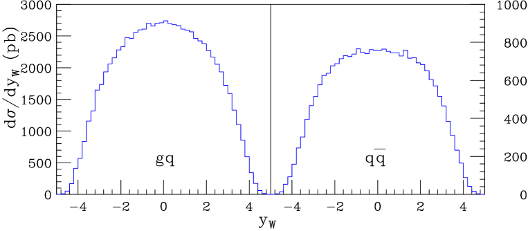
Figure 1: Rapidity distributions of the $W$ boson for the subprocesses $(a)$ $q\,g\to W\,q$ and $(b)$ $q\,\bar{q}\to W\,g$ at the LHC centre-of-mass energy $\sqrt{s}=$ 14 TeV and with $p_{j_{\perp}{\rm min}}=$ 30 GeV.

In case the $W$ boson is produced forward in rapidity, with which rapidity is the jet typically produced ? If the jet is produced in the opposite hemisphere with respect to the $W$ boson, the rapidity interval $|y_{\scriptscriptstyle W}-y_{j}|$ is large, however we know that in this case $W+1$-jet production is strongly suppressed (at LO), since its parton subprocesses can only have quark exchange in the crossed channel, and thus the related production rate falls off with the parton centre-of-mass energy $\hat{s}$. Thus this configuration is dynamically disfavoured. On the other hand, jet production in the same hemisphere as the $W$ boson or centrally in rapidity keeps $x_{a}$ small without substantially increasing $x_{b}$. However, whether the jet is produced in the central region or in the same hemisphere as the $W$ boson depends on the detailed shape of the p.d.f.’s, namely on how large we can afford to make $x_{b}$ while keeping $x_{a}$ small. In Fig. 2 we plot the rapidity distributions of the jet at LHC energies.

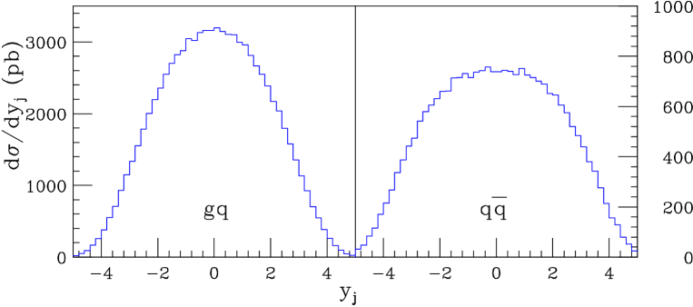
Figure 2: Rapidity distributions of the jet for the subprocesses $(a)$ $q\,g\to W\,q$ and $(b)$ $q\,\bar{q}\to W\,g$ at the LHC centre-of-mass energy $\sqrt{s}=$ 14 TeV and with $p_{j_{\perp}{\rm min}}=$ 30 GeV.

2.2 $W+2$-jet production

Let us consider the hadroproduction of a $W$ boson with two associated jets. At LO the parton subprocesses are

$$(a) g\,g\to W\,q\,\bar{q}\,,$$ (2.2)

$$(b) q\,\bar{q}\to W\,g\,g+W\,q\,{\bar{q}}\,,$$

$$(c) q\,q\to W\,q\,q\,,$$

$$(d) q\,g\to W\,q\,g\,.$$

The momentum fractions of the incoming partons are given through energy-momentum conservation by

$$x_{a} = {|p_{j_{1\perp}}|\over\sqrt{s}}e^{y_{j_{1}}}+{|p_{j_{2\perp}}|\over\sqrt{s}}e^{y_{j_{2}}}+{m_{\perp}\over\sqrt{s}}e^{y_{\scriptscriptstyle W}}\,,$$

$$x_{b} = {|p_{j_{1\perp}}|\over\sqrt{s}}e^{-y_{j_{1}}}+{|p_{j_{2\perp}}|\over\sqrt{s}}e^{-y_{j_{2}}}+{m_{\perp}\over\sqrt{s}}e^{-y_{\scriptscriptstyle W}}\,,$$ (2.3)

with $p_{j_{1,2\perp}}$ the jet transverse momenta and $m_{\perp}=\sqrt{m_{\scriptscriptstyle W}^{2}+|p_{j_{1\perp}}+p_{j_{2\perp}}|^{2}}$ the $W$ transverse mass. For the four subprocesses of Eq. (2.2), the total cross section for the production of a $W$ boson in association with two jets is given in Table 1.

subprocesses	$\sigma(W^{+})$	$\sigma(W^{-})$
$g\,g\to W\,q\,\bar{q}$	170	170
$q\bar{q}\to W\,g\,g+W\,q\,{\bar{q}}$	580	400
$q\,q\to W\,q\,q$	400	300
$q\,g\to W\,q\,g$	3300	2200

Table 1: Total cross sections (pb) for the production of $W^{\pm}$ boson in association with two jets with transverse momentum $p_{j_{1,2\perp}}\geq$ 30 GeV and interjet distance $R(j_{1},j_{2})=\sqrt{(y_{j_{1}}-y_{j_{2}})^{2}+(\phi_{j_{1}}-\phi_{j_{2}})^{2}}\geq$ 0.4 on the rapidity-azimuthal angle plane.

What are the typical rapidity distributions of the $W$ boson and of the two jets? In Figs. 3-6 we plot the rapidity distributions of the $W$ and of the two jets in $W+2$-jet production. The renormalisation and factorisation scales, $\mu_{\scriptscriptstyle R}$ and $\mu_{\scriptscriptstyle F}$, are taken to be equal to $(|p_{j_{1\perp}}|+|p_{j_{2\perp}}|+m_{\perp})/2$. The subprocess $g\,g\to W\,q\,\bar{q}$ is perfectly symmetric, thus the $W$ boson and the two jets are produced mostly in the central rapidity region. However, in the other subprocesses that is not the case: looking at the distributions in $y_{\scriptscriptstyle W}$ (Fig. 3)

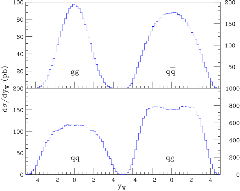
Figure 3: Distributions in $y_{\scriptscriptstyle W}$ for the subprocesses of Eq. (2.2) at the LHC centre-of-mass energy $\sqrt{s}=$ 14 TeV and with $p_{j_{\perp}{\rm min}}=$ 30 GeV.

we see that as we move from $(a)$ to $(d)$ the $W$ boson tends to be produced more and more forward in rapidity. Examining the distributions in $y_{j_{2}}$ (Fig. 4),

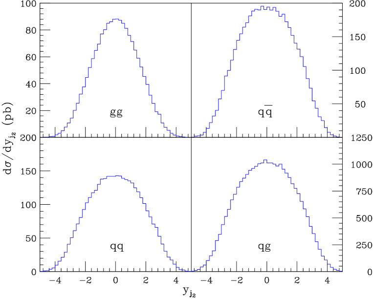
Figure 4: Distributions in $y_{j_{2}}$, where $j_{2}$ is the jet that is closest to the $W$, for the subprocesses of Eq. (2.2) at the LHC centre-of-mass energy $\sqrt{s}=$ 14 TeV and with $p_{j_{\perp}{\rm min}}=$ 30 GeV.

where $j_{2}$ is the jet that is closest to the $W$, we see that this jet tends to follow the $W$ in rapidity. From the distributions in $y_{j_{1}}-y_{j_{2}}$ (Fig. 5),

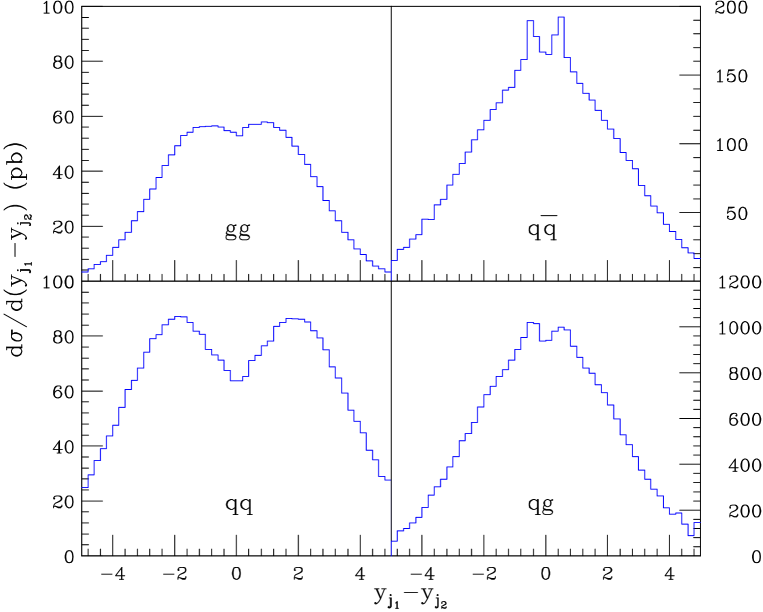
Figure 5: Distributions in $y_{j_{1}}-y_{j_{2}}$ for the subprocesses of Eq. (2.2) at the LHC centre-of-mass energy $\sqrt{s}=$ 14 TeV and with $p_{j_{\perp}{\rm min}}=$ 30 GeV.

we see that in $(a)$ and $(b)$ jet 1 tends to be produced more centrally; in $(d)$ it follows the $W$ boson and jet 2, thus emphasizing the kinematical features already noted in $W+1$-jet production (the twin peaks observed in Fig. 5 in $(a)$, $(b)$ and $(d)$ are due to requiring two jets with interjet distance $R(j_{1},j_{2})\geq$ 0.4); finally in $(c)$ it tends to be produced far in rapidity from the $W$ boson and jet 2.

To understand how these configurations come about, we consider $q\,g\to W\,q\,g$ and follow the analysis of Section 2.1, i.e. we identify $x_{a}$ as the gluon and $x_{b}$ as the quark momentum fractions. To make $x_{a}$ as small as possible at the price of increasing $x_{b}$, the $W$ boson is produced forward (Fig. 3). Note that with respect to Section 2.1 this is made easier by the presence of two jets, which let the $W$ boson have a transverse momentum as small as kinematically possible: ultimately, when the jets are balanced in transverse momentum, the $W$ transverse mass reduces to the mass, $m_{\perp}\to m_{\scriptscriptstyle W}$. In addition, one jet, say $j_{2}$, is always linked to the $W$ boson via a quark propagator as in $W+1$-jet production, so it tends to follow the $W$ in rapidity, as in Fig. 4, however the position of the other jet is a dynamical feature peculiar of $W+2$-jet production: thanks to the gluon exchanged in the crossed channel, that jet can be easily separated in rapidity from the $W$ boson. In $q\bar{q}\to W\,g\,g+W\,q\,{\bar{q}}$, the kinematical mechanism is the same as in $q\,g\to W\,q\,g$ since the antiquark has a sea quark p.d.f., however only $q\bar{q}\to W\,q\,{\bar{q}}$ can have a gluon exchanged in the crossed channel. For $g\,g\to W\,q\,\bar{q}$, which has equal p.d.f.’s for the incoming particles and no gluon exchanged in the crossed channel, we obtain a central distribution, as expected. Note, however, that in Fig. 3 and following the contribution of $g\,g\to W\,q\,\bar{q}$ to $W+2$-jet production is quite small. The $q\,q\to W\,q\,q$ channel is peculiar, since the largest contribution comes from valence-quark distributions, which tend to have rather large $x$’s. In addition, at the dynamical level it features only diagrams with gluon exchange in the crossed channel. Thus to make one $x$ large, it tends to have the $W$ boson and a jet slightly forward in rapidity, while to make the other $x$ large, it has the second jet well forward (and opposite) in rapidity.

Next, we require that the two jets are produced with a sizeable rapidity interval, $|y_{j_{1}}-y_{j_{2}}|\geq 2$, and look at the rapidity distribution of the $W$ boson with respect to the jet average, $y_{\scriptscriptstyle W}-(y_{j_{1}}+y_{j_{2}})/2$ (Fig. 6).

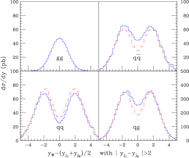
Figure 6: Distributions of the rapidity of $W$ boson with respect to the jet average, $y_{\scriptscriptstyle W}-(y_{j_{1}}+y_{j_{2}})/2$ at $|y_{j_{1}}-y_{j_{2}}|\geq 2$ for the subprocesses of Eq. (2.2) at the LHC centre-of-mass energy $\sqrt{s}=$ 14 TeV and with $p_{j_{\perp}{\rm min}}=$ 30 GeV. The dashed line has been generated by taking the amplitudes in the high-energy limit, as explained after Eq. (4.3).

Now the requirement that the rapidity interval between the jets is large makes the subprocesses with gluon exchange in the crossed channel stand out even more, and the $W$ boson, which is linked to one of the jets by quark exchange in the crossed channel, to follow that jet in rapidity. This is stressed by the double peaks in $(b)$, $(c)$ and $(d)$. Note that the dip between the peaks is maximal for $q\,q\to W\,q\,q$, which features only diagrams with gluon exchange in the crossed channel. Conversely $g\,g\to W\,q\,\bar{q}$ yields the $W$ boson in the central rapidity region and approximately equidistant from the two jets, however it is strongly suppressed since it can only have quark exchange in the crossed channel.

The plots of Fig. 6 are characterised by the dominance of the subprocesses featuring gluon exchange in the crossed channel. The same feature is exhibited by events where we select the jet, say $j_{1}$, that in rapidity is furthest away from the $W$, require that $|y_{\scriptscriptstyle W}-y_{j_{1}}|\geq 2$, and examine the distribution in $y_{\scriptscriptstyle W}-y_{j_{2}}$. Since in this case $j_{2}$ is always linked to the $W$ boson by quark exchange, the distributions are all centered about zero. The leading subprocesses factorise then naturally into two scattering centres: an impact factor for $W+1$-jet production, and an impact factor for jet production. The two impact factors are connected by the gluon exchanged in the crossed channel. Accordingly, the dashed lines of Fig. 6 have been obtained by taking the high-energy limit of the amplitudes featuring crossed-channel gluon exchange (see Eq. (4.3)). On these amplitudes we can then insert the universal leading-logarithmic corrections of ${\cal O}(\alpha_{s}^{n}\ln^{n}(\hat{s}/|\hat{t}|))$, and resum them through the BFKL equation. The impact factor for jet production is known, and we shall summarise its derivation in Section 3.2. The impact factor for $W+1$-jet production is derived in Section 3.3. Next, we summarise jet production at hadron colliders in the high-energy limit.

3 Impact factors

In order to show how to extract the LO impact factor for $W+1$-jet production, we use as a paradigm parton-parton scattering, and the derivation of the LO impact factor for jet production.

3.1 Dijet production at hadron colliders

In the high-energy limit $\hat{s}\gg\hat{t}$, the BFKL theory assumes that any scattering process is dominated by gluon exchange in the crossed channel, which for a given scattering occurs at ${\cal O}(\alpha_{s}^{2})$. This constitutes the leading-order (LO) term of the BFKL resummation. The corresponding QCD amplitude factorizes into a gauge-invariant effective amplitude formed by two scattering centers, the LO impact factors, connected by the gluon exchanged in the crossed channel. The LO impact factors are characteristic of the scattering process at hand. The BFKL equation resums then the universal leading-logarithmic (LL) corrections, of ${\cal O}(\alpha_{s}^{n}\ln^{n}(\hat{s}/|\hat{t}|))$, to the gluon exchange in the crossed channel. These are obtained in the limit of a strong rapidity ordering of the emitted gluon radiation,

$$y_{1}\gg y_{2}\gg\ldots\gg y_{n-1}\gg y_{n}\,.$$ (3.1)

For an arbitrary scattering, the LO term of the BFKL resummation is contained in the higher-order terms of the expansion in $\alpha_{s}$. For dijet production in hadron collisions, the LO term of the BFKL resummation is already included in the LO term of the expansion in $\alpha_{s}$. In this respect, dijet production in hadron collisions at large rapidity intervals is the simplest process to which to apply the BFKL resummation, and thus we shall use it as a paradigm.

Since the cross section for dijet production in the high-energy limit is dominated by gluon exchange in the crossed channel, the functional form of the QCD amplitudes for gluon-gluon, gluon-quark or quark-quark scattering at LO is the same; they differ only by the colour strength in the parton-production vertices. We can then write the cross section,

$$d\sigma=x_{a}f(x_{a},\mu_{F}^{2})\,x_{b}f(x_{b},\mu_{F}^{2})\,d\hat{\sigma}\,,$$ (3.2)

in the following factorised form [22, 23, 24]

$${d\sigma\over d^{2}p_{a^{\prime}_{\perp}}d^{2}p_{b^{\prime}_{\perp}}dy_{a^{\prime}}dy_{b^{\prime}}}\,=\,x_{a}^{0}f_{eff}(x_{a}^{0},\mu_{F}^{2})\,x_{b}^{0}f_{eff}(x_{b}^{0},\mu_{F}^{2})\,{d\hat{\sigma}_{gg}\over d^{2}p_{a^{\prime}_{\perp}}d^{2}p_{b^{\prime}_{\perp}}}\,,$$ (3.3)

where

$$x_{a}^{0}={|p_{a^{\prime}_{\perp}}|\over\sqrt{s}}e^{y_{a^{\prime}}}\,,\qquad\qquad x_{b}^{0}={|p_{b^{\prime}_{\perp}}|\over\sqrt{s}}e^{-y_{b^{\prime}}}\,,$$ (3.4)

are the parton momentum fractions in the high-energy limit, $a^{\prime}$ and $b^{\prime}$ label the forward and backward outgoing jet, respectively, and the effective parton distribution functions are

$$f_{eff}(x,\mu_{F}^{2})=G(x,\mu_{F}^{2})+{4\over 9}\sum_{f}\left[Q_{f}(x,\mu_{F}^{2})+\bar{Q}_{f}(x,\mu_{F}^{2})\right],$$ (3.5)

where the sum is over the quark flavours. In the high-energy limit, the gluon-gluon scattering cross section becomes [22]

$${d\hat{\sigma}_{gg}\over d^{2}p_{a^{\prime}_{\perp}}d^{2}p_{b^{\prime}_{\perp}}}\ =\ \biggl{[}{C_{A}\alpha_{s}\over|p_{a^{\prime}_{\perp}}|^{2}}\biggr{]}\,f(q_{a_{\perp}},q_{b_{\perp}},\Delta y)\,\biggl{[}{C_{A}\alpha_{s}\over|p_{b^{\prime}_{\perp}}|^{2}}\biggr{]}\ ,$$ (3.6)

with $\Delta y=y_{a^{\prime}}-y_{b^{\prime}}$ and $q_{i_{\perp}}$ the momenta transferred in the $t$-channel, with $q_{a_{\perp}}=-p_{a^{\prime}_{\perp}}$ and $q_{b_{\perp}}=p_{b^{\prime}_{\perp}}$, and where $C_{A}=N_{c}=3$. The quantities in square brackets are proportional to the impact factors for jet production. We shall analyse them in Section 3.2. The function $f(q_{a_{\perp}},q_{b_{\perp}},\Delta y)$ is the Green’s function associated with the gluon exchanged in the crossed channel. It is process independent and given in the LL approximation by the solution of the BFKL equation. Its analytic form is,

$$f(q_{a_{\perp}},q_{b_{\perp}},\Delta y)\,={1\over(2\pi)^{2}|q_{a_{\perp}}||q_{b_{\perp}}|}\sum_{n=-\infty}^{\infty}e^{in\phi}\,\int_{-\infty}^{\infty}d\nu\,e^{\omega(\nu,n)\Delta y}\,\left(|q_{a_{\perp}}|^{2}\over|q_{b_{\perp}}|^{2}\right)^{i\nu}\,,$$ (3.7)

with $\phi$ the azimuthal angle between $q_{a}$ and $q_{b}$, and $\omega(\nu,n)$ the eigenvalue of the BFKL equation with maximum at $\omega(0,0)=4\ln{2}C_{A}\alpha_{s}/\pi$. Thus the solution of the BFKL equation resums powers of $\Delta y$, and rises with $\Delta y$ as $f(q_{a_{\perp}},q_{b_{\perp}},\Delta y)\sim\exp(\omega(0,0)\Delta y)$.

3.2 Impact factors for jet production

In the high-energy limit, $\ln(\hat{s}/|\hat{t}|)\gg 1$, the LO QCD amplitudes for gluon-gluon, gluon-quark and quark-quark scattering all factorise into two impact factors for jet production. In order to determine explicitly the impact factors for gluon-jet and for quark-jet production, we shall consider here two of the subprocesses above.

The cross section for the scattering of two gluon into two gluons, $g_{a}\,g_{b}\to g_{a^{\prime}}\,g_{b^{\prime}}$, at LO in the high-energy limit, $\hat{s}=x_{a}^{0}x_{b}^{0}s\gg|\hat{t}|$, can be written as

$$d\hat{\sigma}_{gg} = {1\over\hat{s}}\,\left[{dy_{a^{\prime}}d^{2}p_{a^{\prime}_{\perp}}\over 4\pi}\delta\left(\sqrt{s}x_{a}^{0}\,-\,|p_{a^{\prime}_{\perp}}|e^{y_{a^{\prime}}}\right)\right]$$

$$\times \left[{dy_{b^{\prime}}d^{2}p_{b^{\prime}_{\perp}}\over 4\pi}\delta\left(\sqrt{s}x_{b}^{0}\,-\,|p_{b^{\prime}_{\perp}}|e^{-y_{b^{\prime}}}\right)\right]\delta^{2}(p_{a^{\prime}_{\perp}}+p_{b^{\prime}_{\perp}})\,|{\cal M}_{g\,g\to g\,g}|^{2}\,,$$

where $|{\cal M}_{g\,g\to g\,g}|^{2}$ is the squared tree amplitude, summed (averaged) over final (initial) helicities and colours. The amplitude for gluon-gluon scattering, $g_{a}\,g_{b}\rightarrow g_{a^{\prime}}\,g_{b^{\prime}}$ with all external gluons outgoing, can be written as [25, 26]

$$M^{aa^{\prime}bb^{\prime}\,}_{\nu_{a}\nu_{a^{\prime}}\nu_{b^{\prime}}\nu_{b}}=2\hat{s}\left[ig\,f^{aa^{\prime}c}\,C^{gg}(p_{a}^{\nu_{a}},p_{a^{\prime}}^{\nu_{a^{\prime}}})\right]{1\over\hat{t}}\left[ig\,f^{bb^{\prime}c}\,C^{gg}(p_{b}^{\nu_{b}},p_{b^{\prime}}^{\nu_{b^{\prime}}})\right]\,,$$ (3.9)

where the $\nu$’s label the helicities and the LO vertices $g^{*}\,g\rightarrow g$ are given by

$$C^{gg}(p_{a}^{-},p_{a^{\prime}}^{+})=1\,,\qquad C^{gg}(p_{b}^{-},p_{b^{\prime}}^{+})={p_{b^{\prime}_{\perp}}^{*}\over p_{b^{\prime}_{\perp}}}\,,$$ (3.10)

where we represent the transverse momentum $p_{\perp}$ on the complex plane, $p_{\perp}=p_{x}+ip_{y}$. The functions $C$ transform into their complex conjugates under helicity reversal, $C^{*}(\{k^{\nu}\})=C(\{k^{-\nu}\})$. The helicity-flip function $C(p^{+},p^{\prime+})$ is subleading in the high-energy limit. Thus each function, $C^{gg}$, has only the two helicity configurations of Eq. (3.10) allowed in the high-energy limit.

We define the impact factor, $I(p_{a},p_{a^{\prime}})$ or $I(p_{b},p_{b^{\prime}})$, as the square of each term in squared brackets in Eq. (3.9), summed (averaged) over final (initial) helicities and colours. Thus the LO impact factor for a gluon jet is

$$I^{g}(p_{j},p_{j^{\prime}}) = \frac{1}{2(N_{c}^{2}-1)}\left[ig\,f^{jj^{\prime}c}\,C^{gg}(p_{j}^{\nu_{j}},p_{j^{\prime}}^{\nu_{j^{\prime}}})\right]\left[-ig\,f^{jj^{\prime}c^{\prime}}\,[C^{gg}(p_{j}^{\nu_{j}},p_{j^{\prime}}^{\nu_{j^{\prime}}})]^{*}\right]$$ (3.11)

$$= g^{2}\,{C_{A}\over N_{c}^{2}-1}\,\delta^{cc^{\prime}}\,,$$

with $j=a,b$ and with implicit sums over repeated indices.

From Eq. (3.9) and (3.11), the squared amplitude for gluon-gluon scattering is

$$|{\cal M}_{g\,g\to g\,g}|^{2} = {4\hat{s}^{2}\over\hat{t}^{2}}\,I^{g}(p_{a},p_{a^{\prime}})\,I^{g}(p_{b},p_{b^{\prime}})$$ (3.12)

$$= {4C_{A}^{2}\over N_{c}^{2}-1}\,g^{4}\,{\hat{s}^{2}\over\hat{t}^{2}}={9\over 2}\,g^{4}\,{\hat{s}^{2}\over\hat{t}^{2}}\,.$$

Analogously, the quark-gluon $q_{a}\,g_{b}\rightarrow q_{a^{\prime}}\,g_{b^{\prime}}$ scattering amplitude in the high-energy limit is [26]

$$M^{aa^{\prime}bb^{\prime}\,}_{\nu_{a}\nu_{b}\nu_{b^{\prime}}}=2{\hat{s}}\left[g\,\lambda^{c}_{a^{\prime}\bar{a}}\,C^{\bar{q}q}(p_{a}^{\nu_{a}},p_{a^{\prime}}^{-\nu_{a}})\right]{1\over\hat{t}}\left[ig\,f^{bb^{\prime}c}\,C^{gg}(p_{b}^{\nu_{b}},p_{b^{\prime}}^{\nu_{b^{\prime}}})\right]\,,$$ (3.13)

with LO vertices $g^{*}\,q\rightarrow q$,

$$C^{\bar{q}q}(p_{a}^{-},p_{a^{\prime}}^{+})=-i\,;\qquad C^{\bar{q}q}(p_{b}^{-},p_{b^{\prime}}^{+})=i\,\left({p_{b^{\prime}_{\perp}}^{*}\over p_{b^{\prime}_{\perp}}}\right)^{1/2}\,.$$ (3.14)

Again, each function, $C^{\bar{q}q}$, has two helicity configurations allowed. The LO impact factor for a quark jet is

$$I^{q}(p_{a},p_{a^{\prime}}) = {1\over 2N_{c}}\left[g\,\lambda^{c}_{a^{\prime}\bar{a}}\,C^{\bar{q}q}(p_{a}^{\nu_{a}},p_{a^{\prime}}^{-\nu_{a}})\right]\left[g\,\lambda^{c^{\prime}}_{\bar{a}a^{\prime}}\,[C^{\bar{q}q}(p_{a}^{\nu_{a}},p_{a^{\prime}}^{-\nu_{a}})]^{*}\right]$$ (3.15)

$$= {g^{2}\over 2N_{c}}\,\delta^{cc^{\prime}}\,.$$

The squared amplitude for quark-gluon scattering is then

$$|{\cal M}_{q\,g\to q\,g}|^{2} = {4\hat{s}^{2}\over\hat{t}^{2}}\,I^{q}(p_{a},p_{a^{\prime}})\,I^{g}(p_{b},p_{b^{\prime}})$$ (3.16)

$$= {2C_{A}\over N_{c}}\,g^{4}\,{\hat{s}^{2}\over\hat{t}^{2}}=2\,g^{4}\,{\hat{s}^{2}\over\hat{t}^{2}}\,.$$

Since Eqs.(3.12) and (3.16) only differ by the colour factor 9/4, to calculate the dijet production rate, Eq. (3.3), it suffices to consider one of them, such as gluon-gluon scattering, and include the others through the effective p.d.f. in Eq. (3.5). Using Eq. (3.12) and replacing $\hat{t}^{2}\to|p_{a^{\prime}_{\perp}}^{2}||p_{b^{\prime}_{\perp}}^{2}|$, the cross section for gluon-gluon scattering (3.2) becomes

$${d\hat{\sigma}_{gg}^{0}\over d^{2}p_{a^{\prime}_{\perp}}d^{2}p_{b^{\prime}_{\perp}}}\ =\ \biggl{[}{C_{A}\alpha_{s}\over|p_{a^{\prime}_{\perp}}|^{2}}\biggr{]}\,{1\over 2}\delta^{2}(p_{a^{\prime}_{\perp}}+p_{b^{\prime}_{\perp}})\,\biggl{[}{C_{A}\alpha_{s}\over|p_{b^{\prime}_{\perp}}|^{2}}\biggr{]}\,.$$ (3.17)

At higher orders, powers of $\ln(\hat{s}/|\hat{t}|)$ arise, which can be resummed to all orders in $\alpha_{s}\ln(\hat{s}/|\hat{t}|)$ through the BFKL equation. The term between square brackets in Eq. (3.17) is the LO term of the BFKL resummation. Since in performing the resummation the factorization formula (3.3) holds unchanged, to obtain the resummed parton cross section it suffices to replace the LO term of the BFKL ladder in Eq. (3.17) with the full ladder, thus obtaining Eq. (3.6).

3.3 The impact factor for $W+1$-jet production

In $W+2$-jet production in the limit $|y_{j_{1}}-y_{j_{2}}|\gg 1$ (see Section 2.2), the parton subprocesses $q\,q\to W\,q\,q$ and $q\,g\to W\,q\,g$ and $q\,{\bar{q}}\to W\,q\,{\bar{q}}$ all feature gluon exchange in the crossed channel. Thus the functional form of the corresponding QCD amplitudes is the same. They differ only by the colour strength in the impact factor for jet production, separated from the impact factor for $W$ boson and the other jet by the gluon in the crossed channel. It suffices then to consider only one of the subprocesses above. We shall take $q\,g\to W\,q\,g$ and we shall suppose, for the sake of clarity, that the $W$ boson is produced in the positive-rapidity hemisphere. The subprocesses above factorise according to the kinematics

$$y_{\scriptscriptstyle W}\simeq y_{q}\gg y_{g}\,,\qquad\qquad|p_{\scriptscriptstyle{W_{\perp}}}|\simeq|p_{q_{\perp}}|\simeq|p_{g_{\perp}}|\,.$$ (3.18)

In the high-energy limit, the cross section for $q\,g\to W\,q\,g$ scattering is

$$d\hat{\sigma}_{{\scriptscriptstyle W}qg}={1\over\hat{s}}\,\left[{dy_{\scriptscriptstyle W}d^{2}p_{\scriptscriptstyle W}\over 4\pi(2\pi)^{2}}{dy_{q}d^{2}p_{q_{\perp}}\over 4\pi}\delta\left(\sqrt{s}x_{a}^{0}\,-\,|p_{q_{\perp}}|e^{y_{q}}-m_{\perp}e^{y_{\scriptscriptstyle W}}\right)\right]$$

$$\times \left[{dy_{g}d^{2}p_{g_{\perp}}\over 4\pi}\delta\left(\sqrt{s}x_{b}^{0}\,-\,|p_{g_{\perp}}|e^{-y_{g}}\right)\right]\delta^{2}(p_{{\scriptscriptstyle W}_{\perp}}+p_{q_{\perp}}+p_{g_{\perp}})\,|{\cal M}_{q\,g\to W\,q\,g}|^{2}\,,$$

with the $W$ transverse mass as in Eq. (2.3). If we include the subsequent decay of the $W$ boson into a lepton pair, the kinematics in the high-energy limit becomes

$$y_{e}\simeq y_{\nu}\simeq y_{q}\gg y_{g}\,,\qquad\qquad|p_{e_{\perp}}|\simeq|p_{\nu_{\perp}}|\simeq|p_{q_{\perp}}|\simeq|p_{g_{\perp}}|\,.$$ (3.20)

The cross section for $q\,g\to q\,g\,(W\to)e\,\nu$ scattering can be obtained from Eq. (3.3), replacing the $W$ boson with the lepton pair and using the amplitudes calculated in Refs. [27, 28, 29]. In the notation of Ref. [30] the colour decomposed amplitude is

$${\cal A}_{6}(1_{q},2,3,4_{\bar{q}};5_{\bar{e}},6_{e})$$

$$= g_{W}^{2}g^{2}\,{\cal P}_{W}(s_{56})\,\sum_{\sigma\in S_{2}}(\lambda^{a_{\sigma(2)}}\lambda^{a_{\sigma(3)}})_{i_{1}}^{\bar{i}_{4}}\ A_{6}(1_{q},\sigma(2),\sigma(3),4_{\bar{q}};5_{\bar{e}},6_{e})\,,$$

where legs $1,4$ are the $q\bar{q}$ pair, legs $2,3$ are the gluon legs, and legs 5,6 are the lepton pair; $g_{W}$ is the weak coupling and ${\cal P}_{W}(s)$ the $W$ propagator

$${\cal P}_{W}(s)={1\over s-M_{W}^{2}+i\,\Gamma_{W}\,M_{W}}\,,$$ (3.22)

where $M_{W}$ and $\Gamma_{W}$ are the mass and width of the $W$. The colour ordered subamplitudes are

$$A_{6}(1_{q}^{-},2^{-},3^{+},4_{\bar{q}}^{+},5_{\bar{\ell}}^{+},6_{\ell}^{-})={2\over s_{23}}\,\biggl{[}{\left[1\,3\right]\left\langle 2\,1\right\rangle\left[5\,4\right]\langle\mskip-1.0mu{6}|(1+2)|{3}\mskip-1.0mu\rangle\over\left[2\,1\right]t_{123}}$$

$$- {\left[4\,3\right]\left\langle 2\,4\right\rangle\left\langle 6\,1\right\rangle\langle\mskip-1.0mu{2}|(3+4)|{5}\mskip-1.0mu\rangle\over\left\langle 4\,3\right\rangle t_{234}}-{\langle\mskip-1.0mu{2}|(3+4)|{5}\mskip-1.0mu\rangle\,\langle\mskip-1.0mu{6}|(1+2)|{3}\mskip-1.0mu\rangle\over\left[2\,1\right]\left\langle 4\,3\right\rangle}\biggr{]}\,,$$

$$A_{6}(1_{q}^{-},2^{+},3^{-},4_{\bar{q}}^{+},5_{\bar{\ell}}^{+},6_{\ell}^{-})={2\over s_{23}}\,\biggl{[}-{\left\langle 3\,1\right\rangle^{2}\left[5\,4\right]\langle\mskip-1.0mu{6}|(1+3)|{2}\mskip-1.0mu\rangle\over\left\langle 2\,1\right\rangle t_{123}}$$ (3.23)

$$+ {\left[4\,2\right]^{2}\left\langle 6\,1\right\rangle\langle\mskip-1.0mu{3}|(2+4)|{5}\mskip-1.0mu\rangle\over\left[4\,3\right]t_{234}}+{\left\langle 3\,1\right\rangle\left[4\,2\right]\left\langle 6\,1\right\rangle\left[5\,4\right]\over\left\langle 2\,1\right\rangle\left[4\,3\right]}\biggr{]}\,,$$

with the spinor products defined in Appendix A. The subamplitudes (3.23) are symmetric under the exchange [30]

$$1\leftrightarrow 4\,,\quad 2\leftrightarrow 3\,,\quad 5\leftrightarrow 6\,,\quad\langle ij\rangle\leftrightarrow[ji]\,.$$ (3.24)

In Eq. (3.23) we have neglected the subamplitudes with like-helicity gluons because they are subleading in the high-energy limit.

Next, we make the correspondence $p_{4}\equiv p_{a}$, $p_{1}\equiv p_{a^{\prime}}$, $p_{2}\equiv p_{b}$ and $p_{3}\equiv p_{b^{\prime}}$ and according to Eq. (3.23) we always identify (5)6 as the (anti)lepton momentum. The amplitude for $q_{a}\,g_{b}\to q_{a^{\prime}}\,g_{b^{\prime}}\,(W\to)e\,\nu$ scattering (3.3) in the high-energy limit, $y_{q}\simeq y_{e}\simeq y_{\nu}\gg y_{b^{\prime}}$, is obtained by computing the sub-amplitudes (3.23) in the corresponding kinematics (Appendix B)

$${\cal A}_{q_{a}\,g_{b}\to q_{a^{\prime}}\,g_{b^{\prime}}\,e\,\nu}$$

$$= 2\hat{s}\left[g\,\lambda^{c}_{a^{\prime}\bar{a}}\,C^{\bar{q}q}(p_{a}^{\nu_{a}},p_{q}^{-\nu_{a}},p_{e},p_{\nu},q)\right]{1\over\hat{t}}\left[ig\,f^{bb^{\prime}c}\,C^{gg}(p_{b}^{\nu_{b}},p_{b^{\prime}}^{\nu_{b^{\prime}}})\right]\,,$$

with $p_{b^{\prime}}\equiv p_{g}$, and $q_{\perp}$ the momentum transferred in the crossed channel, $q_{\perp}=p_{b^{\prime}_{\perp}}$, and $\hat{t}\simeq-|q_{\perp}|^{2}$, and the vertex $g^{*}\,d\to u\,e^{-}\,\bar{\nu}$ given by

$$C^{\bar{d}\,u}(p_{a}^{+},p_{q}^{-},p_{e},p_{\nu},q)=\frac{ig_{\scriptscriptstyle W}\,{\cal P}_{W}(s_{\nu e})}{\sqrt{(p^{+}_{q}+p^{+}_{\scriptscriptstyle W}){p^{+}_{\nu}}}}$$

$$\times \left({\langle p_{q}p_{e}\rangle}\,\frac{{p^{+}_{\nu}q_{\perp}^{*}}-\left(p^{+}_{q}+p_{\scriptscriptstyle W}^{+}\right)p_{\nu_{\perp}}^{*}}{t_{abb^{\prime}}}+{\sqrt{\frac{p^{+}_{q}}{p^{+}_{e}}}}\,{p_{\nu_{\perp}}^{*}}\frac{p_{{\scriptscriptstyle W}_{\perp}}p^{+}_{e}+p^{+}_{q}\,p_{e_{\perp}}}{t_{a^{\prime}bb^{\prime}}}\right)\,,$$

with

$$t_{a^{\prime}bb^{\prime}} = (p_{a}+p_{\scriptscriptstyle W})^{2}\simeq{-p^{+}_{q}p_{W}^{-}-|p_{{\scriptscriptstyle W}_{\perp}}|^{2}}\,,$$

$$t_{abb^{\prime}} = (p_{q}+p_{\scriptscriptstyle W})^{2}\,,$$ (3.27)

and with $p_{\scriptscriptstyle W}=p_{e}+p_{\nu}$. In the argument of the vertex in the left-hand side of Eq. (3.3) we do not write explicitly the helicity of the lepton pair, since that is uniquely fixed by the helicity of the quark pair and of the $W$ boson. The vertex $g^{*}\,u\to d\,e^{+}\,\nu$ is obtained from Eq. (3.3) by exchanging $(p_{\nu}\leftrightarrow p_{e})$

$$C^{\bar{u}\,d}(p_{a}^{+},p_{q}^{-},p_{e},p_{\nu},q)=C^{\bar{d}\,u}(p_{a}^{+},p_{q}^{-},p_{\nu},p_{e},q)\,.$$ (3.28)

Using the symmetry (3.24) of the vertex (3.3), we obtain the vertex $g^{*}\,\bar{d}\to\bar{u}\,e^{+}\,\nu$

$$C^{d\,\bar{u}}(p_{a}^{-},p_{q}^{+},p_{e},p_{\nu},q)=-\left[C^{\bar{d}\,u}(p_{a}^{+},p_{q}^{-},p_{e},p_{\nu},q)\right]^{*}\,.$$ (3.29)

The vertex $g^{*}\,\bar{u}\to\bar{d}\,e^{-}\,\bar{\nu}$ is then obtained from Eq. (3.29) by exchanging $(p_{\nu}\leftrightarrow p_{e})$

$$C^{u\,\bar{d}}(p_{a}^{-},p_{q}^{+},p_{e},p_{\nu},q)=C^{d\,\bar{u}}(p_{a}^{-},p_{q}^{+},p_{\nu},p_{e},q)\,.$$ (3.30)

The impact factor for $W+1$-jet production, $I^{q{\scriptscriptstyle W}}$, can be obtained by squaring any of the effective vertices (3.3-3.30) and by integrating out the lepton pair; however, by using Eqs. (3.3) and (3.23) we have computed directly the squared amplitude for $q\,g\to q\,g\,W$ scattering, and compared it to Ref. [31]. Taking then the high-energy limit (3.18), the squared amplitude summed (averaged) over final (initial) colours and helicities, reduces to

$$|{\cal M}_{q\,g\to{\scriptscriptstyle W}\,q\,g}|^{2}=\frac{4\hat{s}^{2}}{\hat{t}^{2}}I^{q{\scriptscriptstyle W}}(p_{a},p_{q},p_{\scriptscriptstyle W},q)I^{g}(p_{b},p_{b^{\prime}})\,,$$ (3.31)

with

$$I^{q{\scriptscriptstyle W}}(p_{a},p_{q},p_{\scriptscriptstyle W},q)=-\frac{\delta^{cc^{\prime}}}{2N_{c}t_{abb^{\prime}}t_{a^{\prime}bb^{\prime}}}g^{2}\frac{g_{\scriptscriptstyle W}^{2}}{2}\left[m_{\scriptscriptstyle W}^{2}\frac{t_{abb^{\prime}}}{t_{a^{\prime}bb^{\prime}}}\left(z+\frac{t_{a^{\prime}bb^{\prime}}}{t_{abb^{\prime}}}\right)^{2}-\hat{t}\left(1+z^{2}\right)\right]\,,$$ (3.32)

where we have defined the momentum fraction

$$z=\frac{p^{+}_{q}}{p^{+}_{q}+p_{\scriptscriptstyle W}^{+}}\,.$$ (3.33)

Using Eq. (3.3) and $\hat{t}\simeq-|q_{\perp}|^{2}$, we can rewrite the impact factor (3.32) as,

$$I^{q{\scriptscriptstyle W}}(p_{a},p_{q},p_{\scriptscriptstyle W},q)$$

$$= -\frac{\delta^{cc^{\prime}}}{2N_{c}t_{abb^{\prime}}t_{a^{\prime}bb^{\prime}}}g^{2}\frac{g_{\scriptscriptstyle W}^{2}}{2}\left[m_{\scriptscriptstyle W}^{2}\frac{\left(-z|q_{\perp}|^{2}+|p_{q_{\perp}}|^{2}-|p_{{\scriptscriptstyle W}_{\perp}}|^{2}\right)^{2}}{t_{abb^{\prime}}t_{a^{\prime}bb^{\prime}}}+|q_{\perp}|^{2}\left(1+z^{2}\right)\right]\,.$$

In the small $|q_{\perp}|$ limit, the jet opposite to the impact factor for $W+1$-jet production becomes collinear, and the cross section obtained from the squared amplitude (3.31) yields an infrared real correction. Since the latter may have at most a logarithmic enhancement as $|q_{\perp}|\to 0$, the squared amplitude (3.31) cannot diverge more rapidly than $1/|q_{\perp}|^{2}$. This entails that in the small $|q_{\perp}|$ limit, the impact factor (3.3) must be at least quadratic in $|q_{\perp}|$, $I^{q{\scriptscriptstyle W}}\sim{\cal O}(|q_{\perp}|^{2})$. Using $q_{\perp}=-(p_{q_{\perp}}+p_{{\scriptscriptstyle W}_{\perp}})$, it is immediate to see that this is the case for Eq. (3.3). In addition, as $q_{\perp}\to 0$ we have an almost on-shell gluon scattering with a quark, then $p_{q_{\perp}}\to-p_{{\scriptscriptstyle W}_{\perp}}$ and averaging over the azimuthal angle of $q_{\perp}$, Eq. (3.3) becomes

$$\lim_{q_{\perp}\to 0}I^{q{\scriptscriptstyle W}} = \frac{\delta^{cc^{\prime}}}{2N_{c}}g^{2}\frac{g_{\scriptscriptstyle W}^{2}}{2}\left(\frac{|q_{\perp}|\,z(1-z)}{|p_{{\scriptscriptstyle W}_{\perp}}|^{2}+zm_{\scriptscriptstyle W}^{2}}\right)^{2}\left[{(1+z^{2})\left(|p_{{\scriptscriptstyle W}_{\perp}}|^{4}+z^{2}m_{\scriptscriptstyle W}^{4}\right)+4z^{2}m_{\scriptscriptstyle W}^{2}|p_{{\scriptscriptstyle W}_{\perp}}|^{2}\over z(|p_{{\scriptscriptstyle W}_{\perp}}|^{2}+zm_{\scriptscriptstyle W}^{2})^{2}}\right]\,$$ (3.35)

$$= 4\delta^{cc^{\prime}}\left(\frac{|q_{\perp}|\,z(1-z)}{|p_{{\scriptscriptstyle W}_{\perp}}|^{2}+zm_{\scriptscriptstyle W}^{2}}\right)^{2}|{\cal M}_{q\,g\to{\scriptscriptstyle W}\,q}|^{2}\,,$$

which explicitly shows that the impact factor is positive definite and that it factorises into the squared amplitude for $q\,g\to W\,q$ scattering [20], as it should.

4 The production rate for $W+2$ jets

In the collision of two hadrons $A$ and $B$, the differential production rate of a $W$ boson with two associated jets is given in terms of the rapidities and transverse momenta by

$${d\sigma\over d^{2}p_{j_{1\perp}}d^{2}p_{j_{2\perp}}d^{2}p_{{\scriptscriptstyle W}_{\perp}}dy_{j_{1}}dy_{j_{2}}dy_{\scriptscriptstyle W}}$$ (4.1)

$$= \sum_{ij}\,x_{a}f_{i/A}(x_{a},\mu_{F}^{2})\,x_{b}f_{j/B}(x_{b},\mu_{F}^{2})\,{|{\cal M}_{ij}|^{2}\over 256\pi^{5}{\hat{s}}^{2}}\,\delta^{2}\left(p_{{\scriptscriptstyle W}_{\perp}}+p_{j_{1\perp}}+p_{j_{2\perp}}\right)\,,$$

with parton momentum fractions (2.3). In Eq. (4.1) the dynamics of the scattering are fully contained in the squared amplitude.

In the limit $|y_{j_{1}}-y_{j_{2}}|\gg 1$, as discussed in Section 3.3, we can identify an outgoing parton with a (anti)quark, while the other, that we called $b^{\prime}$ according to the notation of Section 3.3, can either be a quark or a gluon. The cross section for $W+2$-jet production can be written in the factorised form (3.3), by substituting Eq. (3.31) and using Eq. (3.5),

$${d\sigma\over d^{2}p_{q_{\perp}}d^{2}p_{b^{\prime}_{\perp}}d^{2}p_{{\scriptscriptstyle W}_{\perp}}dy_{q}dy_{b^{\prime}}dy_{\scriptscriptstyle W}}$$ (4.2)

$$= \sum_{i}x_{a}^{0}Q_{i}(x_{a}^{0},\mu_{F}^{2})\,x_{b}^{0}f_{eff}(x_{b}^{0},\mu_{F}^{2}){I^{q{\scriptscriptstyle W}}I^{g}\over 32\pi^{5}|q_{a_{\perp}}|^{2}|q_{b_{\perp}}|^{2}}{\delta^{2}(q_{a_{\perp}}-q_{b_{\perp}})\over 2}\,,$$

where $q_{a_{\perp}}=-p_{q_{\perp}}-p_{{\scriptscriptstyle W}_{\perp}}$ and $q_{b_{\perp}}=p_{b^{\prime}_{\perp}}$, and where we have substituted $\hat{t}^{2}$ with $|q_{a_{\perp}}|^{2}|q_{b_{\perp}}|^{2}$. In the first p.d.f. the sum is over (anti)quark flavours, and the impact factors are given in Eqs. (3.11) and (3.32). The last term is the LO term of the BFKL resummation. Thus, to obtain the BFKL-resummed cross section we just need to replace $\delta^{2}(q_{a_{\perp}}-q_{b_{\perp}})/2$ with $f(q_{a_{\perp}},q_{b_{\perp}},\Delta y)$, as in Eq. (3.7).

However, in Eq. (4.2) energy and longitudinal momentum are not conserved. The parton momentum fractions in the high-energy limit, $x_{a}^{0}$ and $x_{b}^{0}$, given in Eq. (3.3) underestimate the exact ones (2.3) and accordingly the p.d.f.’s can be grossly overestimated. Thus for numerical applications and for a comparison with experimental data, it can be convenient to perform the high-energy limit only on the dynamical part of Eq. (4.1), by writing the squared amplitude in the factorised form (3.31), while leaving the kinematics untouched. This entails

$${d\sigma\over d^{2}p_{q_{\perp}}d^{2}p_{b^{\prime}_{\perp}}d^{2}p_{{\scriptscriptstyle W}_{\perp}}dy_{q}dy_{b^{\prime}}dy_{\scriptscriptstyle W}}$$ (4.3)

$$= \sum_{i}x_{a}Q_{i}(x_{a},\mu_{F}^{2})\,x_{b}f_{eff}(x_{b},\mu_{F}^{2}){1\over 32\pi^{5}}\left[{I^{q{\scriptscriptstyle W}}I^{g}\over\hat{t}^{2}}\right]{\delta^{2}(q_{a_{\perp}}-q_{b_{\perp}})\over 2}\,.$$

For the invariants $\hat{t}$ and $t_{a^{\prime}bb^{\prime}}$, implicit in the square brackets, two options are possible:

• they are taken to be exact, namely $\hat{t}=2p_{b}\cdot p_{b^{\prime}}$ and $t_{a^{\prime}bb^{\prime}}=(p_{a^{\prime}}+p_{\scriptscriptstyle W})^{2}$. For instance, the dashed lines of Fig. 6 have been obtained from Eq. (4.3) with option $(a)$;

• $\hat{t}$ and $t_{a^{\prime}bb^{\prime}}$ are in the high-energy limit, as defined below Eq. (3.3) and in Eq. (3.3) respectively.

Note that Eq. (4.3), with the two approximations for the dynamics above, and Eq. (4.2) have the same theoretical validity, however their numerics may be rather different. In order to examine that in detail, in Fig. 7 we consider $W+2$-jet production as a function of the rapidity interval between the jets $\Delta y=|y_{j_{1}}-y_{j_{2}}|$. For the renormalisation and the factorisation scales we keep the same choice as in Section 2.2.

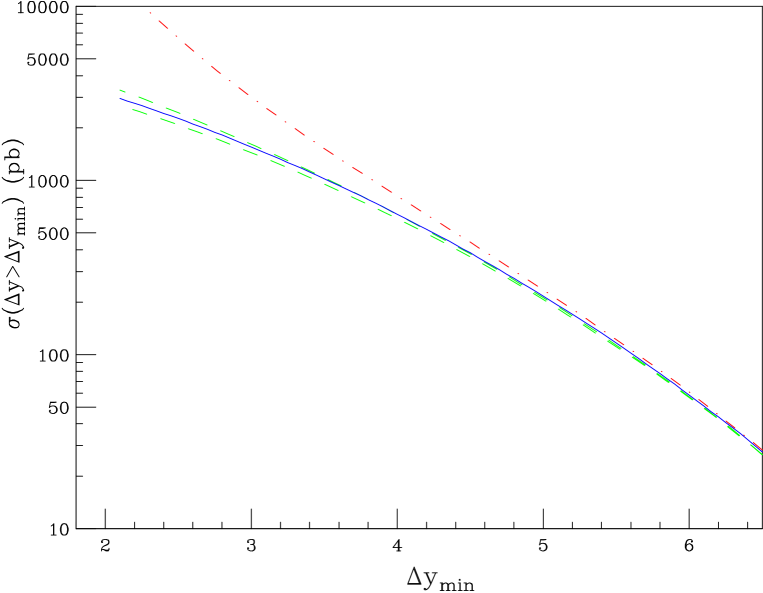
Figure 7: The $W+2$-jet production rate as a function of the rapidity interval between the jets $\Delta y=|y_{j_{1}}-y_{j_{2}}|$. The solid curve is the exact production rate (4.1); the dot-dashed curve is the production rate in the high-energy limit (4.2); the two dashed curves are given by the production rate (4.3), with the two approximations for the dynamics mentioned in the text.

The solid curve is the exact production rate (4.1); the dot-dashed curve is the production rate in the high-energy limit (4.2); the two dashed curves are given by the production rate (4.3), with the two approximations listed above: $(b)$ is the upper dashed curve, and $(a)$ is the lower one. Note that the exact production rate is contained between curves $(a)$ and $(b)$, with $(b)$ yielding the best numerical approximation to the exact curve, while the high-energy limit on the LO kinematics and dynamics (the dot-dashed curve) is rather distant from the exact production rate, unless $\Delta y$ is quite large. The range between curves $(a)$ and $(b)$ may be viewed as a band of uncertainty on the high-energy limit at LO.

5 The BFKL Monte Carlo

In a comparison with experimental data, it must be remembered that the LL BFKL resummation makes some approximations which, even though formally subleading, can be numerically important: $a)$ The BFKL resummation is performed at fixed coupling constant, thus any variation in the scale at which $\alpha_{s}$ is evaluated appears in the next-to-leading-logarithmic (NLL) terms. $b)$ Because of the strong rapidity ordering any two-parton invariant mass is large. Thus there are no collinear divergences in the LL resummation in the BFKL ladder; jets are determined only at tree-level and accordingly have no non-trivial structure. $c)$ Finally, energy and longitudinal momentum are not conserved, since the momentum fraction $x$ of the incoming parton is reconstructed from the kinematic variables of the outgoing partons only, and not including the radiation from the BFKL ladder. Therefore, the BFKL theory can severely underestimate the exact value of the $x$’s, and thus grossly overestimate the parton luminosities. In fact, if a $W$ boson $+\ (n+2)$ partons are produced, we have

$$x_{a(b)}={|p_{j_{1\perp}}|\over\sqrt{s}}e^{(-)y_{j_{1}}}+{|p_{j_{2\perp}}|\over\sqrt{s}}e^{(-)y_{j_{2}}}+{m_{\perp}\over\sqrt{s}}e^{(-)y_{\scriptscriptstyle W}}+\sum_{i=1}^{n}{k_{i\perp}\over\sqrt{s}}e^{(-)y_{i}},$$ (5.1)

where the minus sign in the exponentials of the right-hand side applies to the subscript $b$ on the left-hand side. In the BFKL theory, the LL approximation and the kinematics (3.1) imply that in the determination of $x_{a}$ ($x_{b}$) only the first (last) term in Eq. (5.1) is kept. The terms neglected in Eq.(3.4) are formally subleading. However, a comparison of three-parton production with the exact kinematics (5.1) to the truncation of the BFKL ladder to ${\cal O}(\alpha_{s}^{3})$ shows that the LL approximation entails sizable violations of energy-momentum conservation [32].

Kinematic cuts and constraints like Eq. (5.1) can be implemented in the BFKL framework by unfolding the BFKL integral equation, resulting in an explicit sum over the number of emitted gluons. Each term in this sum is then a phase space integral over the BFKL gluon phase space, which allows for a BFKL Monte Carlo to be constructed [33, 34]. Since each emitted BFKL gluon enters the calculation with an explicit phase space integral, this approach allows for the running of the coupling to be included into the BFKL solution, and also for the gluon radiation to be taken into account in Eq. (5.1).

The first step in this procedure is to transform the relevant Green’s function $f(\vec{q}_{a\perp},\vec{q}_{b\perp},\Delta y)$ of Eq. (3.7) to moment space via

$$f(\vec{q}_{a\perp},\vec{q}_{b\perp},\Delta y)\ =\ \int{d\omega\over 2\pi i}\,e^{\omega\Delta y}\,f_{\omega}(\vec{q}_{a\perp},\vec{q}_{b\perp})\,.$$ (5.2)

We can then write the BFKL equation as

$$\omega\,f_{\omega}(\vec{q}_{a\perp},\vec{q}_{b\perp})\,={1\over 2}\,\delta(\vec{q}_{a\perp}-\vec{q}_{b\perp})\,+\,{\bar{\alpha}_{s}\over\pi}\int{d^{2}\vec{k}_{\perp}\over k_{\perp}^{2}}\,K(\vec{q}_{a\perp},\vec{q}_{b\perp},\vec{k}_{\perp})\,,$$ (5.3)

where the kernel $K$ is given by

$$K(\vec{q}_{a\perp},\vec{q}_{b\perp},\vec{k}_{\perp})=f_{\omega}(\vec{q}_{a\perp}+\vec{k}_{\perp},\vec{q}_{b\perp})-{q_{a\perp}^{2}\over k_{\perp}^{2}+(\vec{q}_{a\perp}+\vec{k}_{\perp})^{2}}\,f_{\omega}(\vec{q}_{a\perp},\vec{q}_{b\perp})\,,$$ (5.4)

and $\bar{\alpha}_{s}=\alpha_{s}\frac{N_{c}}{\pi}$. The first term in the kernel accounts for the emission of a real gluon of transverse momentum $\vec{k}_{\perp}$ and the second term accounts for the virtual radiative corrections.

We now separate the $\vec{k}_{\perp}$ integral in (5.3) into ‘resolved’ and ‘unresolved’ contributions, according to whether $|\vec{k}_{\perp}|$ lie above or below a small transverse energy scale $\mu$. The scale $\mu$ is assumed to be small compared to the other relevant scales in the problem (such as the minimum transverse momentum, for instance). The virtual and unresolved contributions are then combined into a single, finite integral. The BFKL equation becomes

$$\omega\,f_{\omega}(\vec{q}_{a\perp},\vec{q}_{b\perp})\! = \!{1\over 2}\,\delta(\vec{q}_{a\perp}-\vec{q}_{b\perp})\,+\,{\bar{\alpha}_{s}\over\pi}\int_{k_{\perp}^{2}>\mu^{2}}{d^{2}\vec{k}_{\perp}\over k_{\perp}^{2}}\,f_{\omega}(\vec{q}_{a\perp}+\vec{k}_{\perp},\vec{q}_{b\perp})$$ (5.5)

$$+ \!\!\!\!{\bar{\alpha}_{s}\over\pi}\int{d^{2}\vec{k}_{\perp}\over k_{\perp}^{2}}\left[f_{\omega}(\vec{q}_{a\perp}+\vec{k}_{\perp},\vec{q}_{b\perp})\,\theta(\mu^{2}-k_{\perp}^{2})\,-\,{q_{a\perp}^{2}\,f_{\omega}(\vec{q}_{a\perp},\vec{q}_{b\perp})\over k_{\perp}^{2}+(\vec{q}_{a\perp}+\vec{k}_{\perp})^{2}}\right]$$

The combined unresolved/virtual integral can be simplified by noting that since $k_{\perp}^{2}\ll q_{a\perp}^{2},q_{b\perp}^{2}$ by construction, the $\vec{k}_{\perp}$ term in the argument of $f_{\omega}$ can be neglected, giving

$$(\omega-\omega_{0})\,f_{\omega}(\vec{q}_{a\perp},\vec{q}_{b\perp})\,=\,{1\over 2}\,\delta(\vec{q}_{a\perp}-\vec{q}_{b\perp})\,+\,{\bar{\alpha}_{s}\over\pi}\int_{k_{\perp}^{2}>\mu^{2}}{d^{2}\vec{k}_{\perp}\over k_{\perp}^{2}}\,f_{\omega}(\vec{q}_{a\perp}+\vec{k}_{\perp},\vec{q}_{b\perp})\\ \,,$$

where

$$\omega_{0}={\bar{\alpha}_{s}\over\pi}\int{d^{2}\vec{k}_{\perp}\over k_{\perp}^{2}}\left[\theta(\mu^{2}-k_{\perp}^{2})\,-\,{q_{a\perp}^{2}\over\vec{k}_{\perp}^{2}+(\vec{q}_{a\perp}+\vec{k}_{\perp})^{2}}\right]\simeq{\bar{\alpha}_{s}}\,\ln\left({\mu^{2}\over q_{a\perp}^{2}}\right)\,.$$ (5.6)

The virtual and unresolved contributions are now contained in $\omega_{0}$ and we are left with an integral over resolved real gluons. Eq. (5) is now solved iteratively, and performing the inverse transform we have

$$f(\vec{q}_{a\perp},\vec{q}_{b\perp},\Delta y)\,=\,\sum_{n=0}^{\infty}f^{(n)}(\vec{q}_{a\perp},\vec{q}_{b\perp},\Delta y)\,,$$ (5.7)

where

$$f^{(0)}(\vec{q}_{a\perp},\vec{q}_{b\perp},\Delta y) = \left[\frac{\mu^{2}}{q_{a\perp}^{2}}\right]^{\bar{\alpha}_{s}\Delta y}\,\,\frac{1}{2}\,\delta(\vec{q}_{a\perp}-\vec{q}_{b\perp})\,,$$

$$f^{(n\geq 1)}(\vec{q}_{a\perp},\vec{q}_{b\perp},\Delta y) = \left[\frac{\mu^{2}}{q_{a\perp}^{2}}\right]^{\bar{\alpha}_{s}\Delta y}\,\left\{\prod_{i=1}^{n}\int d^{2}\vec{k}_{i\perp}\,dy_{i}\,{\cal F}_{i}\right\}\,\frac{1}{2}\,\delta(\vec{q}_{a\perp}-\vec{q}_{b\perp}-\sum_{i=1}^{n}\vec{k}_{i\perp})\,,$$

$${\cal F}_{i} = \frac{\bar{\alpha}_{s}}{\pi k_{i\perp}^{2}}\,\theta(k_{i\perp}^{2}-\mu^{2})\,\theta(y_{i-1}-y_{i})\,\left[{(\vec{q}_{a\perp}+\sum_{j=1}^{i-1}\vec{k}_{j\perp})^{2}\over(\vec{q}_{a\perp}+\sum_{j=1}^{i}\vec{k}_{j\perp})^{2}}\right]^{\bar{\alpha}_{s}y_{i}}\,.$$ (5.8)

Thus the solution to the BFKL equation is recast in terms of phase space integrals for resolved gluon emissions, with form factors representing the net effect of unresolved and virtual emissions. In this way, each $f^{(n)}$ depends on the resolution parameter $\mu$, whereas the full sum $f$ does not.

The derivation given above only applies for fixed coupling because we have left $\alpha_{s}$ outside the integrals. The modifications necessary to account for a running coupling $\alpha_{s}(k_{i\perp}^{2})$ are straightforward [33]. In the rest of this paper, we will however discuss only the fixed coupling version of the BFKL Monte Carlo with the coupling entering the BFKL equation set to $\alpha_{s}(p_{j_{\perp}{\rm min}}^{2})$, and with energy momentum conservation built in through Eq. (5.1). The effects of including the BFKL gluon radiation in the Bjorken $x$’s are far bigger than the effects of the running coupling, which amount to an approximately 10% effect in the cross section of Fig. 8.

Figure 8: The $W+2$-jet production rate as a function of the rapidity interval between the jets $\Delta y=|y_{j_{1}}-y_{j_{2}}|$, with acceptance cuts $y_{\scriptscriptstyle W},\,y_{j_{2}}\geq 1$ and $y_{j_{1}}\leq-1$, or $y_{\scriptscriptstyle W},\,y_{j_{2}}\leq-1$ and $y_{j_{1}}\geq 1$. The diamonds are the exact production rate (4.1); the dashed curve is the production rate in the high-energy limit (4.3) with option $(a)$; the dotted curve is the same with option $(b)$; the solid curve includes the BFKL corrections.

6 BFKL observables

After having considered several approximations to the high-energy limit and introduced the BFKL Monte Carlo as the tool that we shall use to analyse the BFKL gluon radiation, we turn now to the analysis of the effects of the BFKL radiation on some physical observables. From Eq. (3.7) we see that in order to detect evidence of a BFKL-type behaviour in a scattering process, we need to obtain $\Delta y$ as large as possible. In the context of dijet production this can be done by minimizing the jet transverse energy, and maximizing the parton centre-of-mass energy $\hat{s}$. Since $\hat{s}=x_{a}x_{b}s$, in a fixed-energy collider this is achieved by increasing the parton momentum fractions $x_{a,b}$, and then measuring the dijet production rate $d\sigma/d\Delta y$. However, in dijet production three effects hinder the characteristic growth of the BFKL ladder (3.7) with respect to LO production:

• as the $x$’s grow the parton luminosities fall off, making it difficult to disentangle the eventual BFKL-driven rise of the parton cross section from the p.d.f.’s fall off [23, 24];

• the implementation of the exact $x$’s (5.1) in the BFKL Monte Carlo [35], rather than using $x^{0}_{a,b}$ (3.4) as prescribed by the high-energy limit, shifts the p.d.f.’s toward smaller values, and thus further suppresses the production rate. This effect is already present at ${\cal O}(\alpha_{s}^{3})$ [32];

• in dijet production both the tagged jets have typically the same minimum transverse energy; at NLO, the dijet cross section as a function of the difference $\cal D$ between the minimum transverse energies of the two jets turns out to have a slope $d\sigma/d\cal D$ which is infinite at ${\cal D}=0$ [36, 37]. This hints to the presence of large logarithms of Sudakov type, which can conceal the logarithms of type $\ln(\hat{s}/\hat{t})$ characteristic of the BFKL dynamics.

The combination of these three effects changes drastically the shape of dijet production $d\sigma/d\Delta y$ as a function of the rapidity interval between the tagged jets, showing a depletion [35] rather than the characteristic increase of the BFKL analytic solution.

In Fig. 8 we consider $W+2$-jet production as a function of $\Delta y$, and with acceptance cuts $y_{\scriptscriptstyle W},\,y_{j_{2}}\geq 1$ and $y_{j_{1}}\leq-1$, or $y_{\scriptscriptstyle W},\,y_{j_{2}}\leq-1$ and $y_{j_{1}}\geq 1$. For all of the curves of Figs. 8-12, we choose $\mu_{\scriptscriptstyle R1}=p_{j_{1\perp}}$ and $\mu_{\scriptscriptstyle R2}=(p_{j_{2\perp}}+m_{\perp})/2$ as renormalisation scales, and $\mu_{\scriptscriptstyle F1}=\mu_{\scriptscriptstyle F2}=(|p_{j_{1\perp}}|+|p_{j_{2\perp}}|+m_{\perp})/2$ as factorisation scales. We justify the peculiar scale choices above as follows: we note that our calculations are at LO (from the renormalisation point of view), thus the scale choice is completely arbitrary, as long as it is physically unambiguous. However, a uniform choice for all of the curves in the same figure is required for a consistent comparison between different approximations. In addition, in the high-energy limit the impact factors for $W+1$-jet production on one side and for jet production on the other can be viewed as two almost independent scattering centres linked by a gluon exchanged in the crossed channel, thus it makes sense to run $\alpha_{s}$ according to the scale set by each impact factor. Accordingly, in the LO calculation $\alpha_{s}^{2}$ must be understood as $\alpha_{s}(p_{j_{1\perp}}^{2})\,\alpha_{s}\left((p_{j_{2\perp}}+m_{\perp})^{2}/4\right)$. In the high-energy limit it is possible (and would make sense) to choose the factorisation scales equal to the renormalisation scales, however for the exact production rate this choice would not be physically sensible since no high-energy factorisation is present, thus for the factorisation scales we keep the same choice as in the previous figures. In Fig. 8 the diamonds represent the exact production rate (4.1); the dashed curve is the production rate in the high-energy limit (4.3) with option $(a)$; the dotted curve is the same with option $(b)$; the solid curve includes the BFKL corrections. In Figs. 8-12 we have computed the BFKL corrections using Eq. (4.3) with option $(b)$. However, the particular option we choose is immaterial since the uncertainty related to the choice of option in Eq. (4.3) is much smaller than the uncertainties intrinsic to the BFKL resummation, the latter being due to the leading-log approximation, the choice of scale of $\alpha_{s}$ and the approximation on the incoming parton momentum fractions. Note that the curve of Fig. 8 is both qualitatively and quantitatively different from $d\sigma/d\Delta y$ in dijet production: the peak in Fig. 8 is a striking confirmation of the dominance of the configurations asymmetric in rapidity, discussed in Section 2.2. In fact the symmetric acceptance cut strongly penalises the asymmetric configurations when $\Delta y$ approaches its minimum value; since the asymmetric configurations dominate the $W+2$-jet production rate, the effect is a strong depletion of the latter. In addition, the BFKL ladder (solid curve), which includes energy-momentum conservation (5.1), shows a substantial increase of the cross section with respect to the LO analysis (dotted and dashed curves), as opposed to a decrease in the dijet case. To understand how this comes about, we note that the presence of at least three particles in the final state makes the threshold configurations, and thus the logarithms of Sudakov type, much less compelling than in the dijet case. Secondly, the implementation of the kinematic constraint (5.1) in the BFKL Monte Carlo, rather than using $x^{0}_{a,b}$ (3.3) in the high-energy limit, has a much lesser impact than in the dijet case. This is due to the fact that the valence quark distribution in $q\,g\to q\,g\,W$ is much less sensitive to $x$ variations than the gluon distribution in $g\,g\to g\,g$.

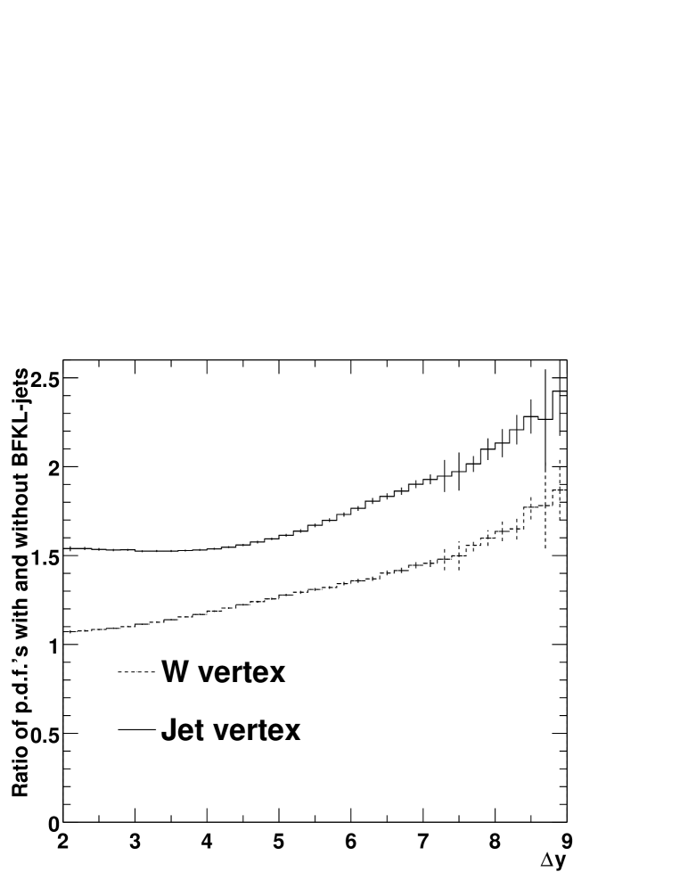
Figure 9: The ratio $f(x^{0},\mu_{\scriptscriptstyle F}^{2})/f(x,\mu_{\scriptscriptstyle F}^{2})$ of the p.d.f. as a function of the $x^{0}$’s (3.3) in the high-energy limit versus the p.d.f. as a function of the exact $x$ (5.1); the dashed-dotted curve is the ratio $f(x_{a}^{0},\mu_{\scriptscriptstyle F}^{2})/f(x_{a},\mu_{\scriptscriptstyle F}^{2})$, and the solid curve is the ratio $f_{eff}(x_{b}^{0},\mu_{\scriptscriptstyle F}^{2})/f_{eff}(x_{b},\mu_{\scriptscriptstyle F}^{2})$.

To analyse this more precisely, we consider in Fig. 9 the ratio $f(x^{0},\mu_{\scriptscriptstyle F}^{2})/f(x,\mu_{\scriptscriptstyle F}^{2})$ of the p.d.f. as a function of the $x^{0}$’s (3.3) in the high-energy limit versus the p.d.f. as a function of the exact $x$ (5.1). The ratio is calculated for each event in the Monte Carlo as the ratio of the p.d.f. evaluated at $x^{0}$ compared to an evaluation at $x$, weighted with the contribution of this event to the cross section according to (4.3) with option $(b)$ and the BFKL ladder added. Finally, this distribution is binned in $\Delta y$. To be definite, since the high-energy factorisation entails that each impact factor is associated to one of the two incoming partons, we can term the ratio $f(x_{a}^{0},\mu_{\scriptscriptstyle F}^{2})/f(x_{a},\mu_{\scriptscriptstyle F}^{2})$ as the one associated to the impact factor for $W+1$-jet production, and the ratio $f_{eff}(x_{b}^{0},\mu_{\scriptscriptstyle F}^{2})/f_{eff}(x_{b},\mu_{\scriptscriptstyle F}^{2})$ as the one associated to the impact factor for jet production. As we see from Fig. 9, the solid curve is much farther away from 1 than the dashed-dotted curve. Since the effective p.d.f. is dominated by the gluon distribution, this implies that the ratio $f_{eff}(x_{b}^{0},\mu_{\scriptscriptstyle F}^{2})/f_{eff}(x_{b},\mu_{\scriptscriptstyle F}^{2})$ is much more sensitive to variations of the $x$’s than the ratio $f(x_{a}^{0},\mu_{\scriptscriptstyle F}^{2})/f(x_{a},\mu_{\scriptscriptstyle F}^{2})$, which is made by valence quark distributions. Accordingly, we obtain a smaller depletion of the BFKL Monte Carlo prediction in $W+2$-jet production as compared to dijet production. In addition, both the curves in Fig. 9 rise as $\Delta y$ grows. That entails that the BFKL radiation, which enters the determination of the $x$’s in the denominator, yields as expected a contribution which is growing with $\Delta y$.

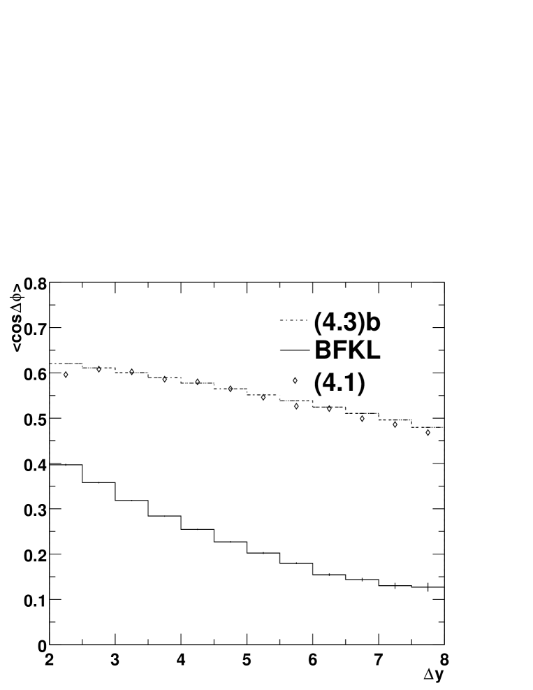
Figure 10: The average azimuthal angle $\langle\cos\Delta\phi\rangle$, where $\Delta\phi=|\phi_{j_{1}}-\phi_{j_{2}}|-\pi$, as a function of the rapidity interval between the jets $\Delta y=|y_{j_{1}}-y_{j_{2}}|$, with acceptance cuts $y_{\scriptscriptstyle W},\,y_{j_{2}}\geq 1$ and $y_{j_{1}}\leq-1$, or $y_{\scriptscriptstyle W},\,y_{j_{2}}\leq-1$ and $y_{j_{1}}\geq 1$. The diamonds are the exact production rate (4.1); the dashed-dotted curve is the production rate in the high-energy limit (4.3) with option $(b)$; the solid curve includes the BFKL corrections.

A variable that has been extensively studied as possibly sensitive to BFKL effects is the azimuthal angle decorrelation $\Delta\phi=|\phi_{j_{1}}-\phi_{j_{2}}|-\pi$ between the most forward and backward jets in inclusive dijet samples. At LO the jets are supposed to be back to back, with a correlation which is smeared by gluon radiation induced by parton showers and hadronization. However, if we look at the correlation also as a function of $\Delta y$, we expect the gluon radiation between the jets to further blur the information on the mutual position in transverse momentum space, and thus the decorrelation to grow with $\Delta y$. From Eq. (3.7), we see that the BFKL-induced gluon radiation might account for that [23, 24, 32, 33, 38]. The decorrelation between the tagging jets has been analysed, and indeed observed, by the D0 Collaboration in dijet production at the Tevatron Collider [1]. However, the BFKL-induced radiation predicts a stronger decorrelation than the data, even though the BFKL Monte Carlo [33] shows a much more realistic azimuthal decorrelation than the BFKL analytic solution. The data are correctly reproduced by the HERWIG Monte Carlo generator [39, 40, 41], which includes parton showers and hadronization. This suggests that the azimuthal angle decorrelation $\Delta\phi$, picking up preferentially configurations where the tagged jets are back to back, is sensitive to threshold configurations, and thus to logarithms of Sudakov type, even more than it is in the inclusive dijet production rate $d\sigma/d\Delta y$ [37, 42]. However, as discussed in the paragraph above, in $W+2$-jet production we expect the logarithms of Sudakov type to play a much less significant role. Thus, in analogy with dijet production, in Fig. 10 we consider the average azimuthal angle $\langle\cos\Delta\phi\rangle$ as a function of the rapidity interval between the jets $\Delta y$. The acceptance cuts are the same as for Fig. 8. The diamonds are the exact production rate (4.1); the dashed-dotted curve is the production rate in the high-energy limit (4.3) with option $(b)$; the solid curve includes the BFKL corrections. The average azimuthal angle being defined as a ratio of production rates is much less sensitive to scale variations than the curves of Fig. 8.

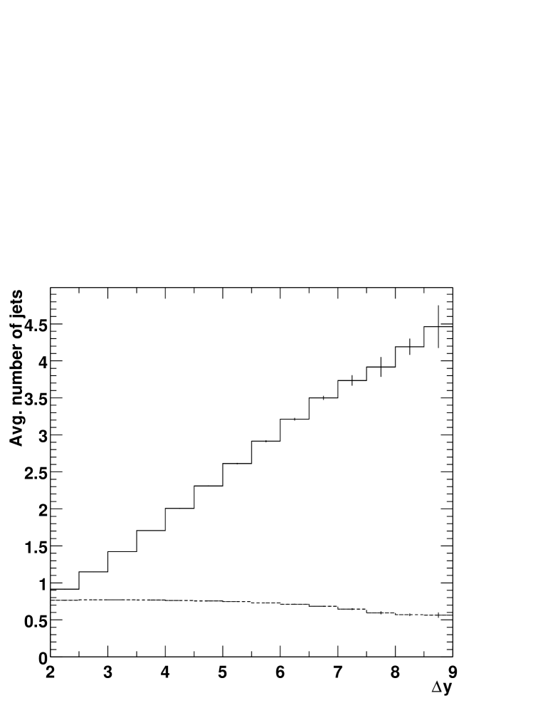
Figure 11: Solid: the BFKL prediction for the mean number of jets $\langle n\rangle$ with $p_{\perp}>p_{j\perp\rm min}=30$ GeV as a function of the rapidity interval between the jets $\Delta y=|y_{j_{1}}-y_{j_{2}}|$. Dotted: the same in the rapidity range $-1<y_{j}<1$.

In Fig. 11 we plot the BFKL prediction for the mean number of jets $\langle n\rangle$ with $p_{\perp}>p_{j\perp\rm min}=30$ GeV, emitted by the BFKL ladder as a function of the rapidity interval between the jets $\Delta y$, and the BFKL prediction for the same variable in the rapidity range $-1<y_{j}<1$. We see that the mean number of jets rises approximately linearly with $\Delta y$, and accordingly that the mean number of jets in the rapidity range $-1<y_{j}<1$ stays constant. We can crudely understand this, by noting that for a very large $\Delta y$ the cross section from Eqs. (3.7) and (4.2) behaves like

$$\sigma|_{\Delta y}\sim e^{\omega(0,0)\Delta y}=\sum_{n=0}^{\infty}{(\omega(0,0)\Delta y)^{n}\over n!}\,,$$ (6.1)

with $\omega(0,0)=4\ln{2}C_{A}\alpha_{s}/\pi$, and a power of $\alpha_{s}$ for each real correction to, and therefore for each emitted gluon from, the BFKL ladder. Up to corrections of type $\ln(p_{\perp}/p_{j\perp\rm min})$ [34], the mean number of jets emitted by the BFKL ladder is then

$$\langle n\rangle={(n\sigma)|_{\Delta y}\over\sigma|_{\Delta y}}\simeq\omega(0,0)\Delta y\,.$$ (6.2)

For $\alpha_{s}(p_{j\perp\rm min}^{2})$ with $p_{j\perp\rm min}=30$ GeV, this yields typically a jet each second unit of rapidity, which is in rough agreement with Fig. 11.

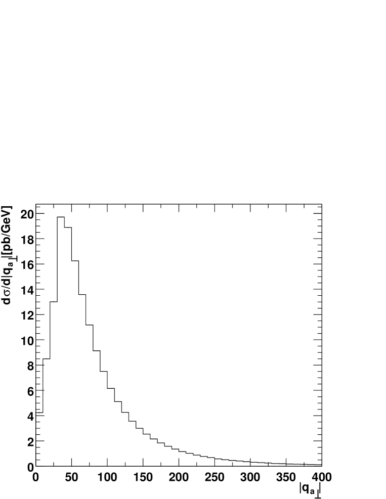
Figure 12: The $W+2$-jet production rate, including BFKL corrections, as a function of the transverse momentum $q_{a_{\perp}}$, with $q_{a_{\perp}}=-(p_{q_{\perp}}+p_{{\scriptscriptstyle W}_{\perp}})$.

Finally, in Fig. 12 we consider $W+2$-jet production as a function of the transverse momentum $q_{a_{\perp}}=-(p_{q_{\perp}}+p_{{\scriptscriptstyle W}_{\perp}})$ exiting from the impact factor $I^{q{\scriptscriptstyle W}}$ for $W+1$-jet production. At LO, $q_{a_{\perp}}=q_{b_{\perp}}=p_{b^{\prime}_{\perp}}$, thus $q_{a_{\perp}}$ is bound to be equal to the transverse momentum of the jet opposite to the impact factor $I^{q{\scriptscriptstyle W}}$ (and thus to be always larger than 30 GeV). In presence of the gluon radiation of the BFKL ladder, this is not longer true, and $q_{a_{\perp}}$ is allowed to go to zero. However, a simple power-counting argument shows that the production rate is finite as $q_{a_{\perp}}\to 0$. In fact from Eq. (3.3) we know that $I^{q{\scriptscriptstyle W}}\sim{\cal O}(|q_{a_{\perp}}|^{2})$. Substituting it, and the ladder (3.7) which goes like ${\cal O}(1/|q_{a_{\perp}}|)$, in Eq. (4.2), we see that as far as the behaviour in $q_{a_{\perp}}$ is concerned,

$${d\sigma\over dq_{a_{\perp}}^{2}}\sim{q_{a_{\perp}}^{2}\over q_{a_{\perp}}^{3}}\delta^{2}(q_{a_{\perp}}+p_{q_{\perp}}+p_{{\scriptscriptstyle W}_{\perp}})\,,$$ (6.3)

and therefore the distribution $d\sigma/dq_{a_{\perp}}$ is finite as $q_{a_{\perp}}\to 0$, in agreement with Fig. 12.

7 Conclusions

In Section 2 we have examined the exact LO inclusive rapidity distribution for $W+1$-jet and $W+2$-jet production; as for the latter, we have seen that the dominant parton sub-process $q\,g\to q\,g\,W$ produces a great deal of $W$ bosons forward in rapidity. This is due to the different shape of the p.d.f.’s of the incoming quark and gluon, and to gluon exchange in the crossed channel which loosens the bound between the $W$ boson and a jet on one (rapidity) side, and the other jet on the other side. In Section 3 we have derived the impact factor for $W+1$-jet production, both as a function of the $W$-boson momentum and including the leptonic decay of the $W$ boson. In Section 4 we have compared several high-energy approximations at LO to the exact production rate. The range between the most extreme high-energy approximations may be considered as the theoretical uncertainty on the high-energy limit at LO.

In Section 6 we have considered some BFKL footprints, most notably the rate $d\sigma/d\Delta y$ and the azimuthal angle decorrelation $d\sigma/d\Delta\phi$ as functions of the rapidity interval $\Delta y$ between two tagged jets. These observables had already been considered in inclusive dijet production, however because of the dominance of the configurations asymmetric in rapidity and the presence of at least three particles in the final state, which makes threshold configurations less relevant, in $W+2$-jet production $d\sigma/d\Delta y$ and $d\sigma/\Delta\phi$ take on a completely new light. In addition, we have considered the mean number of jets, which as expected rises approximately linearly with $\Delta y$. Finally, we have computed the transverse momentum distribution of the impact factor for $W+1$-jet production. At LO this is bound from below by momentum conservation at the minimum transverse energy of the jet opposite to the $W+1$-jet configuration, but with additional gluon radiation it is allowed to reach zero, where the distribution is finite.

Finally, we note that one of the leading contributions to the $WW+2$-jet production rate in the high-energy limit is obtained by convoluting two impact factors for $W+1$-jet production with a gluon exchanged in the crossed channel. The analysis of this process, in the exact case, in the high-energy limit and with BFKL corrections is left for future investigations [43].

Appendix A Multiparton kinematics

We consider the production of a $W(\to e\nu)$ and two jets of momenta $p_{a^{\prime}}$ and $p_{b^{\prime}}$, in the scattering between two partons of momenta $p_{a}$ and $p_{b}$ ($p_{a}^{0}<0$ and $p_{b}^{0}<0$).

Using light-cone coordinates $p^{\pm}=p_{0}\pm p_{z}$, and complex transverse coordinates $p_{\perp}=p^{x}+ip^{y}$, with scalar product $2p\cdot q=p^{+}q^{-}+p^{-}q^{+}-p_{\perp}q^{*}_{\perp}-p^{*}_{\perp}q_{\perp}$, the 4-momenta are,

$$p_{a} = \left(p_{a}^{+}/2,0,0,p_{a}^{+}/2\right)=\left(p_{a}^{+},0;0,0\right)\,,$$

$$p_{b} = \left(p_{b}^{-}/2,0,0,-p_{b}^{-}/2\right)=\left(0,p_{b}^{-};0,0\right)\,,$$ (A.1)

$$p_{i} = \left((p_{i}^{+}+p_{i}^{-})/2,{\rm Re}[p_{i_{\perp}}],{\rm Im}[p_{i_{\perp}}],(p_{i}^{+}-p_{i}^{-})/2\right)$$

$$= \left(|p_{i_{\perp}}|e^{y_{i}},|p_{i_{\perp}}|e^{-y_{i}};|p_{i_{\perp}}|\cos{\phi_{i}},|p_{i_{\perp}}|\sin{\phi_{i}}\right)\,\,,\;i=3(b^{\prime}),4(a^{\prime}),5(\bar{\ell}),6(\ell)\,$$

where the first notation is the standard representation $p^{\mu}=(p^{0},p^{x},p^{y},p^{z})$, while in the second we have the + and - components to the left of the semicolon , and to the right the transverse components. $y$ is the parton rapidity and $\phi$ is the azimuthal angle between the vector $p_{\perp}$ and an arbitrary vector in the transverse plane. From the momentum conservation ($i=b^{\prime},a^{\prime},{\bar{\ell}},\ell$),

$$0 = \sum_{i=3}^{6}p_{i_{\perp}}\,,$$

$$p_{a}^{+} = -\sum_{i=3}^{6}p_{i}^{+}\,,$$ (A.2)

$$p_{b}^{-} = -\sum_{i=3}^{6}p_{i}^{-}\,,$$

the Mandelstam invariants may be written as,

$$\hat{s}_{ij} = 2p_{i}\cdot p_{j}=p_{i}^{+}p_{j}^{-}+p_{i}^{-}p_{j}^{+}-p_{i_{\perp}}p_{j_{\perp}}^{*}-p_{i_{\perp}}^{*}p_{j_{\perp}}\,.$$

so that

$$\hat{s} = 2p_{a}\cdot p_{b}=\sum_{i,j=3}^{6}p_{i}^{+}p_{j}^{-}\,,$$

$$\hat{s}_{ai} = 2p_{a}\cdot p_{i}=-\sum_{j=3}^{6}p_{i}^{-}p_{j}^{+}\,,$$ (A.3)

$$\hat{s}_{bi} = 2p_{b}\cdot p_{i}=-\sum_{j=3}^{6}p_{i}^{+}p_{j}^{-}.$$

The spinor products are defined as

$$\langle p_{i}-|p_{j}+\rangle \equiv \langle ij\rangle\,,$$

$$\langle p_{i}+|p_{j}-\rangle \equiv \left[ij\right]\,,$$ (A.4)

$$\langle p_{i}-|/\!\!\!p_{k}|p_{j}-\rangle \equiv \langle i|k|j\rangle\,.$$

Using the above spinor representation, the spinor products for the momenta (A.1) are

$$\langle p_{i}p_{j}\rangle = p_{i_{\perp}}\sqrt{p_{j}^{+}\over p_{i}^{+}}-p_{j_{\perp}}\sqrt{p_{i}^{+}\over p_{j}^{+}}\,,$$

$$\langle p_{a}p_{i}\rangle = -i\sqrt{-p_{1}^{+}\over p_{i}^{+}}\,p_{i_{\perp}}\,,$$ (A.5)

$$\langle p_{i}p_{b}\rangle = i\sqrt{-p_{b}^{-}p_{i}^{+}}\,,$$

$$\langle p_{a}p_{b}\rangle = -\sqrt{\hat{s}}\,,$$

where we have used the mass-shell condition $|p_{i_{\perp}}|^{2}=p_{i}^{+}p_{i}^{-}$. The spinor products fulfill the identities ($i\equiv p_{i},j\equiv p_{j}$),

$$\langle ij\rangle = -\langle ji\rangle\,,$$

$$\left[ij\right] = -\left[ji\right]\,,$$

$$\langle ij\rangle^{*} = {\rm sign}(p^{0}_{i}p^{0}_{j})\left[ji\right]\,,$$

$$\left(\langle i+|\gamma^{\mu}|j+\rangle\right)^{*} = {\rm sign}(p^{0}_{i}p^{0}_{j})\langle j+|\gamma^{\mu}|i+\rangle,$$ (A.6)

$$\langle ij\rangle\left[ji\right] = 2p_{i}\cdot p_{j}=\hat{s}_{ij}\,,$$

$$\langle i+|/\!\!\!k|j+\rangle = \left[ik\right]\langle kj\rangle,$$

$$\langle i-|/\!\!\!k|j-\rangle = \langle ik\rangle\left[kj\right]\,.$$

Appendix B Next-to-leading corrections in the forward-rapidity region

We consider the production of particles $p_{a}^{\prime}$, $p_{e}$, $p_{\nu}$ in the forward-rapidity region of parton $p_{a}$,

$$y_{q}\simeq y_{e}\simeq y_{\nu}\gg y_{b^{\prime}};\qquad|p_{e_{\perp}}|\simeq|p_{\nu_{\perp}}|\simeq|p_{q_{\perp}}|\simeq|p_{b^{\prime}_{\perp}}|\,,$$ (B.1)

Momentum conservation (A.2) simply generalizes to,

$$p_{a}^{+} \simeq -(p_{q}^{+}+p_{e}^{+}+p_{\nu}^{+})\,,$$ (B.2)

$$p_{b}^{-} \simeq -p_{b^{\prime}}^{-}\,.$$ (B.3)

and accordingly the Mandelstam invariants (A.3) may be written as,

$$\hat{s} = 2p_{a}\cdot p_{b}\,\simeq\,(p_{q}^{+}+p_{e}^{+}+p_{\nu}^{+})p_{b^{\prime}}^{-}\,,$$

$$\hat{u} = 2p_{a}\cdot p_{b^{\prime}}\,\simeq\,-(p_{q}^{+}+p_{e}^{+}+p_{\nu}^{+})p_{b^{\prime}}^{-}\,,$$

$$\hat{u}_{k} = 2p_{b}\cdot p_{k}\,\simeq\,-p_{k}^{+}p_{b^{\prime}}^{-}\,,\qquad k=q,e,\nu$$

$$\hat{t}_{k} = 2p_{a}\cdot p_{k}\,\simeq\,-(p_{q}^{+}+p_{e}^{+}+p_{\nu}^{+})p_{k}^{-}\,,\qquad k=q,e,\nu$$ (B.4)

$$\hat{t} = 2p_{b}\cdot p_{b^{\prime}}\,\simeq\,-|p_{b^{\prime}_{\perp}}|^{2}\,,$$

to leading accuracy. The spinor products (A.5) become

$$\langle p_{a}p_{b}\rangle = -\sqrt{\hat{s}}\simeq-\sqrt{(p_{q}^{+}+p_{e}^{+}+p_{\nu}^{+})p_{b^{\prime}}^{-}}\,,$$

$$\langle p_{a}p_{b^{\prime}}\rangle = -i\sqrt{-p_{a}^{+}\over p_{b^{\prime}}^{+}}\,p_{b^{\prime}_{\perp}}\simeq i{p_{b^{\prime}_{\perp}}\over|p_{b^{\prime}_{\perp}}|}\langle p_{a}p_{b}\rangle\,,$$

$$\langle p_{a}p_{k}\rangle = -i\sqrt{-p_{a}^{+}\over p_{k}^{+}}\,p_{k_{\perp}}\simeq-i\sqrt{p_{q}^{+}+p_{e}^{+}+p_{\nu}^{+}\over p_{k}^{+}}p_{k_{\perp}}\,,\qquad\qquad k=q,e,\nu$$

$$\langle p_{k}p_{b}\rangle = i\sqrt{-p_{b}^{-}p_{k}^{+}}\,\simeq i\sqrt{p_{k}^{+}p_{b^{\prime}}^{-}}\,,\qquad k=q,e,\nu$$

$$\langle p_{b^{\prime}}p_{b}\rangle = i\sqrt{-p_{b}^{-}p_{b^{\prime}}^{+}}\,\simeq i|p_{b^{\prime}_{\perp}}|\,,$$

$$\langle p_{k}p_{b^{\prime}}\rangle = p_{k_{\perp}}\sqrt{p_{b^{\prime}}^{+}\over p_{k}^{+}}-p_{b^{\prime}_{\perp}}\sqrt{p_{k}^{+}\over p_{b^{\prime}}^{+}}\simeq-p_{b^{\prime}_{\perp}}\,\sqrt{p_{k}^{+}\over p_{b^{\prime}}^{+}}\,,\qquad k=q,e,\nu\,.$$

References

- [1] S. Abachi et al. [D0 Collaboration], Phys. Rev. Lett. 77 (1996) 595 [hep-ex/9603010].
- [2] B. Abbott et al. [D0 Collaboration], Phys. Rev. Lett. 84 (2000) 5722 [hep-ex/9912032].
- [3] S. Aid et al. [H1 Collaboration], Phys. Lett. B 356 (1995) 118 [hep-ex/9506012].
- [4] J. Breitweg et al. [ZEUS Collaboration], Eur. Phys. J. C 6 (1999) 239 [hep-ex/9805016].
- [5] C. Adloff et al. [H1 Collaboration], Nucl. Phys. B 538 (1999) 3 [hep-ex/9809028].
- [6] M. Acciarri et al. [L3 Collaboration], Phys. Lett. B 453 (1999) 333.
- [7] S. Abachi et al. [D0 Collaboration], Phys. Rev. Lett. 72 (1994) 2332.
- [8] S. Abachi et al. [D0 Collaboration], Phys. Rev. Lett. 76 (1996) 734 [hep-ex/9509013].
- [9] F. Abe et al. [CDF Collaboration], Phys. Rev. Lett. 74 (1995) 855.
- [10] M. Derrick et al. [ZEUS Collaboration], Phys. Lett. B 369 (1996) 55 [hep-ex/9510012].
- [11] E. A. Kuraev, L. N. Lipatov and V. S. Fadin, Sov. Phys. JETP45 (1977) 199 [Zh. Eksp. Teor. Fiz. 72 (1977) 199].
- [12] I. I. Balitsky and L. N. Lipatov, Sov. J. Nucl. Phys. 28 (1978) 822 [Yad. Fiz. 28 (1978) 822].
- [13] J. F. Gunion, A. Stange and S. Willenbrock, “Weakly-coupled Higgs bosons”, [hep-ph/9602238].
- [14] R. N. Cahn and S. Dawson, Phys. Lett. B 136 (1984) 196 [Erratum-ibid. B 138 (1984) 196].
- [15] R. N. Cahn, S. D. Ellis, R. Kleiss and W. J. Stirling, Phys. Rev. D 35 (1987) 1626.
- [16] Y. L. Dokshitzer, S. I. Troian and V. A. Khoze, Sov. J. Nucl. Phys. 46 (1987) 712 [Yad. Fiz. 46 (1987) 712].
- [17] J. D. Bjorken, Phys. Rev. D 47 (1993) 101.
- [18] V. Barger, R. J. Phillips and D. Zeppenfeld, Phys. Lett. B 346 (1995) 106 [hep-ph/9412276].
- [19] T. Stelzer and W. F. Long, Comput. Phys. Commun. 81, 357 (1994) [hep-ph/9401258].
- [20] R. K. Ellis, W. J. Stirling and B. R. Webber, QCD and collider physics, Cambridge Univ. Press.
- [21] A. D. Martin, R. G. Roberts, W. J. Stirling and R. S. Thorne, Eur. Phys. J. C 4, 463 (1998) [hep-ph/9803445].
- [22] A. H. Mueller and H. Navelet, Nucl. Phys. B 282 (1987) 727.
- [23] V. Del Duca and C. R. Schmidt, Phys. Rev. D 49 (1994) 4510 [hep-ph/9311290].
- [24] W. J. Stirling, Nucl. Phys. B 423 (1994) 56 [hep-ph/9401266].
- [25] V. Del Duca, Phys. Rev. D 52 (1995) 1527 [hep-ph/9503340].
- [26] V. Del Duca, “Next-to-leading corrections to the BFKL equation”, [hep-ph/9605404].
- [27] J. F. Gunion and Z. Kunszt, Phys. Lett. B 161 (1985) 333.
- [28] R. Kleiss and W. J. Stirling, Nucl. Phys. B 262 (1985) 235.
- [29] R. K. Ellis and R. J. Gonsalves, in Super-Collider Physics, ed. D.E. Soper (World Scientific, Singapore, 1986).
- [30] Z. Bern, L. Dixon and D. A. Kosower, Nucl. Phys. B 513 (1998) 3 [hep-ph/9708239].
- [31] M. Mangano and S. Parke, Phys. Rev. D 41 (1990) 59.
- [32] V. Del Duca and C. R. Schmidt, Phys. Rev. D 51 (1995) 2150 [hep-ph/9407359].
- [33] L. H. Orr and W. J. Stirling, Phys. Rev. D 56 (1997) 5875 [hep-ph/9706529].
- [34] C. R. Schmidt, Phys. Rev. Lett. 78, 4531 (1997) [hep-ph/9612454].
- [35] L. H. Orr and W. J. Stirling, Phys. Lett. B 429 (1998) 135 [hep-ph/9801304].
- [36] S. Frixione and G. Ridolfi, Nucl. Phys. B 507 (1997) 315 [hep-ph/9707345].
- [37] J. R. Andersen, V. Del Duca, S. Frixione, C. R. Schmidt and W. J. Stirling, JHEP0102 (2001) 007 [hep-ph/0101180].
- [38] V. Del Duca and C. R. Schmidt, Nucl. Phys. Proc. Suppl. 39BC (1995) 137 [hep-ph/9408239].
- [39] G. Marchesini and B. R. Webber, Nucl. Phys. B 310 (1988) 461.
- [40] I. G. Knowles, Nucl. Phys. B 310 (1988) 571.
- [41] G. Marchesini, B. R. Webber, G. Abbiendi, I. G. Knowles, M. H. Seymour and L. Stanco, Comput. Phys. Commun. 67 (1992) 465.
- [42] Y. L. Dokshitzer, hep-ph/9801372. Plenary talk at the International Europhysics Conference on High-Energy Physics (HEP 97), Jerusalem, Israel, 1997.
- [43] J.R. Andersen, V. Del Duca, F. Maltoni and W.J. Stirling, in progress.