BA-01-21

Realistic Supersymmetric $SU(6)$

Qaisar Shafi^a  and  Zurab Tavartkiladze^b

^aBartol Research Institute, University of Delaware, Newark, DE 19716, USA

^b Institute of Physics, Georgian Academy of Sciences, 380077 Tbilisi, Georgia

We present an example of SUSY $SU(6)$ GUT, which predicts an excellent value for $\alpha_{s}(M_{Z})(\simeq 0.119)$, in comparison with the value $\alpha_{s}^{0}(M_{Z})\simeq 0.126$ of minimal SUSY $SU(5)$. A crucial role is played by the vectorlike multiplets from the matter sector, whose masses lie below the GUT scale. For a realistic pattern of fermion masses, the adjoint scalar of $SU(6)$ has VEV along the $SU(4)\times SU(2)\times U(1)$ direction. This also offers a natural resolution of the doublet-triplet (DT) splitting through the pseudo Goldstone Boson mechanism.

The minimal SUSY $SU(5)$ model suffers from a variety of nagging problems. For instance, the measured value of the strong coupling $\alpha_{s}(M_{Z})=0.119\pm 0.002$ [1], while the predicted value is $\alpha_{s}^{0}=0.126$ [2]. It also predicts the wrong asymptotic relations $m_{s}^{(0)}=m_{\mu}^{(0)}$, $m_{d}^{(0)}/m_{s}^{(0)}=m_{e}^{(0)}/m_{\mu}^{(0)}$. And finally, although SUSY guarantees stability of scales against radiative corrections, the origin of DT splitting remains unexplained. In attempting to resolve these problems, one can either consider some extended versions of $SU(5)$ or an alternative GUT scenario. In fact, for obtaining a desirable value of $\alpha_{s}(M_{Z})$, some additional states below the GUT scale could play an important role [3, 4]. For realistic fermion masses, either a scalar $45$ plet [5] or additional fermionic states [4] can be introduced. Within $SU(5)$, solution of the DT splitting problem requires a rather complicated $(50+\overline{50}+75)$ set of scalars, which turn out to be crucial for realization of the missing partner mechanism [6]. Replacing $SU(5)$ with $SO(10)$, one can achieve DT splitting through the missing VEV mechanism [7]. Very attractive and promising scenarios are those in which the light higgs doublets emerge as pseudo-Goldstone Bosons (PGB). This idea is easily realized within $SU(6)$ [9, 10], $SU(3)\times SU(3)\times SU(3)$ [11, 12] or flipped $SU(6)$ [13] models. Also, $SU(6)$ scenarios with additional custodial symmetries can provide a natural understanding of DT splitting [14].

In this letter we show how these three problems could be simultaneously resolved by considering an $SU(6)$ GUT. The value of $\alpha_{s}(M_{Z})$, it turns out, is closely tied with the matter sector, and is expressed through some asymptotic mass relations. It is interesting to note that a realistic pattern of fermion masses unequivocally requires the VEV of the adjoint higgs to be along the $SU(4)\times SU(2)\times U(1)$ direction. This also permits realization of the PGB mechanism [9, 10, 11] for achieving a natural DT splitting.

Consider the SUSY $SU(6)$ GUT with chiral ‘matter’ multiplets $15+\bar{6}+\bar{6}\hskip 1.13809pt^{\prime}$ per generation. In terms of $SU(5)$: $15=10+5$, $\bar{6}=\bar{5}+1$ (and same for $\bar{6}\hskip 1.13809pt^{\prime}$). Thus, we have the additional $SU(5)$ $\bar{5}+5$ vectorlike states, which decouple after $SU(6)$ breaking. At first glance, since they are complete $SU(5)$ plets, one may think that the picture of gauge coupling unification will not be altered at one loop level. However, it turns out that the doublet and triplet fragments from these additional $5$ ($\bar{5}$) plets are split in mass. This happens because, in order to get a realistic pattern of down quark and charged lepton masses, we somehow must remove the degeneracy between their mass matrices. If this is done, then the heavy vectorlike doublet and triplet states also will acquire different masses, and their ratios will be expressed through asymptotic mass relations of down quarks and charged leptons, giving rise to the possibility of predicting $\alpha_{s}(M_{Z})$.

The relevant $SU(6)$ invariant couplings, in lowest order, are of the form $15(\bar{6}+\bar{6}\hskip 1.13809pt^{\prime})\bar{H}$, where $\bar{H}$ ($H$) is an antisextet (sextet) scalar field. In order to avoid the wrong asymptotic relations $m_{s}^{(0)}=m_{\mu}^{(0)}$, $m_{d}^{(0)}/m_{s}^{(0)}=m_{e}^{(0)}/m_{\mu}^{(0)}$ we will insert in these couplings the $SU(6)$ adjoint scalar $\Sigma(35)$ [this can be realized through a $Z_{2}$ symmetry $\Sigma\to-\Sigma$, $(\bar{6},\bar{6}\hskip 1.13809pt^{\prime})\to-(\bar{6},\bar{6}\hskip 1.13809pt^{\prime})$]. For a transparent demonstration, let us first consider the case of one generation. The relevant couplings are:

$$\frac{1}{M}15_{ij}\Sigma^{\hskip 1.13809pti}_{m}\left(\alpha\hskip 1.13809pt\bar{6}^{\hskip 1.13809ptm}\bar{H}^{\hskip 1.13809ptj}+\beta\hskip 1.13809pt\bar{6}^{\hskip 1.13809ptj}\bar{H}^{\hskip 1.13809ptm}+\alpha\hskip 1.13809pt^{\prime}\hskip 1.13809pt\bar{6}^{\prime\hskip 1.13809ptm}\bar{H}^{\hskip 1.13809pt\hskip 1.13809ptj}+\beta\hskip 1.13809pt^{\prime}\hskip 1.13809pt\bar{6}^{\prime\hskip 1.13809ptj}\bar{H}^{\hskip 1.13809ptm}\right)~{},$$ (1)

where $i,j,m$ are $SU(6)$ indices, $\alpha,\dots,\beta\hskip 1.13809pt^{\prime}$ - are dimensionless couplings, and $M$ is some cutoff mass scale. $\Sigma$ and $\bar{H}$ have VEVs of the same order ($\sim M_{G}$), and the light higgs doublet $h_{d}$ is suppressed by equal weights in these plets. It is easy to verify that the relevant terms are built with the higgs doublet $h_{d}$ extracted from $\bar{H}$, and we will ignore terms in which the doublets from $\Sigma$ participate (such terms do not lead to light fermion masses to be identified as quarks and leptons, will couple with decoupled states). From (1), we have:

$$\begin{array}[]{cc}&{\begin{array}[]{cc}\!\!\!d^{\hskip 0.56905ptc}{}{}{}{}{}{}{}{}{}{}{}{}{}{}{}{}&\,\,~{}~{}~{}d^{\hskip 0.56905ptc}\hskip 1.13809pt{}^{\prime}{}{}{}{}\end{array}}\\ \vspace{2mm}\hat{M}_{D}=\begin{array}[]{c}q\\ \\ \bar{d}^{\hskip 0.56905ptc}\par\end{array}\!\!\!\!\!\!\!\!&{\left(\begin{array}[]{cc}\!\!\!\,(\alpha\Sigma_{c}-\beta\Sigma_{w})h_{d}~{}~{},&\!\!\!\!\,(\alpha\hskip 1.13809pt^{\prime}\hskip 1.13809pt\Sigma_{c}-\beta\hskip 1.13809pt^{\prime}\hskip 1.13809pt\Sigma_{w})h_{d}\\ \\ \!\!\!\,(\alpha\Sigma_{c}-\beta\Sigma_{6})v~{}~{},&\!\!\!\!\,(\alpha\hskip 1.13809pt^{\prime}\hskip 1.13809pt\Sigma_{c}-\beta\hskip 1.13809pt^{\prime}\hskip 1.13809pt\Sigma_{6})v\par\end{array}\!\!\right)\!\frac{1}{M}}~{},\end{array}\!\!~{}~{}~{}$$ (2)

$$\begin{array}[]{cc}&{\begin{array}[]{cc}\!\!\!l{}{}{}{}{}{}{}{}{}{}{}{}{}{}{}{}&\,\,~{}~{}~{}l\hskip 1.13809pt^{\prime}{}{}{}{}\end{array}}\\ \vspace{2mm}\hat{M}_{E}=\begin{array}[]{c}e^{c}\\ \\ \bar{l}\par\end{array}\!\!\!\!\!\!\!\!&{\left(\begin{array}[]{cc}\!\!\!\,(\alpha-\beta)\Sigma_{w}h_{d}~{}~{},&\!\!\!\!\,(\alpha\hskip 1.13809pt^{\prime}\hskip 1.13809pt-\beta\hskip 1.13809pt^{\prime}\hskip 1.13809pt)\Sigma_{w}h_{d}\\ \\ \!\!\!\,(\alpha\Sigma_{w}-\beta\Sigma_{6})v~{}~{},&\!\!\!\!\,(\alpha\hskip 1.13809pt^{\prime}\hskip 1.13809pt\Sigma_{w}-\beta\hskip 1.13809pt^{\prime}\hskip 1.13809pt\Sigma_{6})v\par\end{array}\!\!\right)\!\frac{1}{M}}~{},\end{array}\!\!~{}~{}~{}$$ (3)

where $15\supset(q,e^{c},\bar{l},u^{c})$, $\bar{6}\supset(d^{c},l)$, $\bar{6}\hskip 1.13809pt^{\prime}\supset(d^{c}\hskip 1.13809pt{}^{\prime},l\hskip 1.13809pt^{\prime})$, and for the scalar VEVs $\langle\bar{H}\rangle\equiv v$, $\langle\Sigma\rangle={\rm Diag}(\Sigma_{c},\Sigma_{c},\Sigma_{c},\Sigma_{w},\Sigma_{w},\Sigma_{6})$, with $\Sigma_{6}=-3\Sigma_{c}-2\Sigma_{w}$. From (2), (3) we see that pairs of doublet and triplet states decouple with masses $\sim v\langle\Sigma\rangle/M$, while the light down quark and charged lepton’s masses are $\sim h_{d}\langle\Sigma\rangle/M$. More precisely, from (2), (3),

$${\rm Det}(\hat{M}_{D})=\frac{v}{M^{2}}\Sigma_{c}(\Sigma_{w}-\Sigma_{6})(\alpha\beta\hskip 1.13809pt^{\prime}-\beta\alpha\hskip 1.13809pt^{\prime})h_{d}~{},$$

$${\rm Det}(\hat{M}_{E})=\frac{v}{M^{2}}\Sigma_{w}(\Sigma_{w}-\Sigma_{6})(\alpha\beta\hskip 1.13809pt^{\prime}-\beta\alpha\hskip 1.13809pt^{\prime})h_{d}~{}.$$ (4)

From (4) [and also from (2), (3)] it is obvious that the symmetry breaking patterns $SU(5)\times U(1)$ and $SU(3)\times SU(3)\times U(1)$ are not plausible, since, in these cases, we either have degeneracy between $\hat{M}_{D}$ and $\hat{M}_{E}$ or the determinants in (4) are zero [in the latter case some quark and lepton states are massless]. We therefore conclude that the only possible $\langle\Sigma\rangle$ VEV which can lead to a realistic fermion mass pattern is $SU(4)\times SU(2)\times U(1)($e.g. $\Sigma_{c}=\Sigma_{6}=-\Sigma_{w}/2$)

$$\langle\Sigma\rangle={\rm Diag}(1,1,1,-2,-2,1)\cdot V~{}.$$ (5)

Using (5) in (4), one obtains

$${\rm Det}(\hat{M}_{E})=-2\cdot{\rm Det}(\hat{M}_{D})~{},$$ (6)

which implies $m_{e}^{(0)}M^{l}=2m_{d}^{(0)}M^{d^{c}}$, where $M^{l}$, $M^{d^{c}}$ are the masses of the heavy doublet and triplet components respectively, and $m_{e}^{(0)}$, $m_{d}^{(0)}$ denote the asymptotic values of charged lepton and down quark mases. Therefore,

$$\frac{M^{l}}{M^{d^{c}}}=2\frac{m_{d}^{(0)}}{m_{e}^{(0)}}~{}.$$ (7)

Knowing the asymptotic value of $\frac{m_{d}^{(0)}}{m_{e}^{(0)}}$ for a given generation, we calculate through (7) the ratio $M^{l}/M^{d^{c}}$. The latter give us possibility to predict the value of $\alpha_{s}(M_{Z})$.

Analagous results can be obtained for the case with three generations, and as we will see, even inclusion of intergeneration mixings do not modify the picture. Instead of (2), (3) we will have $6\times 6$ matrices. Using (5), the appropriate mass matrices are:

$$\begin{array}[]{cc}&{\begin{array}[]{cc}{}{}\hfil&{}{}{}{}{}\hfil\end{array}}\\ \vspace{2mm}\begin{array}[]{c}\\ \\ \end{array}\!\!\!\!\!\!\!\!&{\hat{\cal M}_{D}\!=\!\!\left(\begin{array}[]{cc}\!\!\!\,(\hat{\alpha}\!+\!2\hat{\beta})h_{d}~{}\hskip 0.85358pt,&\!\!\!\!\,(\hat{\alpha}\hskip 1.13809pt^{\prime}\hskip 1.13809pt\!+\!2\hat{\beta}\hskip 1.13809pt^{\prime}\hskip 1.13809pt)h_{d}\\ \\ \!\!\!\,(\hat{\alpha}\!-\!\hat{\beta})v~{}~{},&\!\!\!\!\,(\hat{\alpha}\hskip 1.13809pt^{\prime}\hskip 1.13809pt\!-\!\hat{\beta}\hskip 1.13809pt^{\prime}\hskip 1.13809pt)v\end{array}\!\!\right)\!\frac{V}{M}}\hskip 0.56905pt,\!\par\end{array}\!\!\begin{array}[]{cc}&{\begin{array}[]{cc}{}\hfil&{}{}{}{}{}{}\hfil\end{array}}\\ \vspace{2mm}\begin{array}[]{c}\\ \end{array}\!\!\!\!\!\!\!\!\!\!&{\hat{\cal M}_{E}\!=\!\!\left(\begin{array}[]{cc}\!\!\!\,2(\hat{\beta}\!-\!\hat{\alpha})h_{d}~{}\hskip 1.42262pt,&\!\!\!\!\,2(\hat{\beta}\hskip 1.13809pt^{\prime}\hskip 1.13809pt\!-\!\hat{\alpha}\hskip 1.13809pt^{\prime}\hskip 1.13809pt)h_{d}\\ \\ \!\!\!\,-\!(2\hat{\alpha}\!+\!\hat{\beta})v~{}~{},&\!\!\!\!\,-\!(2\hat{\alpha}\hskip 1.13809pt^{\prime}\hskip 1.13809pt\!+\!\hat{\beta}\hskip 1.13809pt^{\prime}\hskip 1.13809pt)v\end{array}\!\!\right)\!\frac{V}{M}}\hskip 1.13809pt,\par\par\end{array}~{}~{}~{}$$ (8)

where $\hat{\alpha},\dots,\hat{\beta}\hskip 1.13809pt^{\prime}$ indicate $3\times 3$ matrices in generation space.

It is not difficult to find a relation between the determinants of matrices in (8). Recall that determinants remain unchanged by making some linear manipulations with their rows and coulomns. More precisely:

$$\begin{array}[]{cc}&{\begin{array}[]{cc}{}{}\hfil&{}{}{}{}{}\hfil\end{array}}\\ \vspace{2mm}\begin{array}[]{c}\\ \\ \end{array}\!\!\!\!\!\!\!\!&{{\rm Det}(\hat{\cal M}_{D})\!=\!\left|\begin{array}[]{cc}\!\!\!\,(\hat{\alpha}\!+\!2\hat{\beta})h_{d}~{}\hskip 0.85358pt,&\!\!\!\!\,(\hat{\alpha}\hskip 1.13809pt^{\prime}\hskip 1.13809pt\!+\!2\hat{\beta}\hskip 1.13809pt^{\prime}\hskip 1.13809pt)h_{d}\\ \\ \!\!\!\,(2\hat{\alpha}\!+\!\hat{\beta})v~{}~{},&\!\!\!\!\,(2\hat{\alpha}\hskip 1.13809pt^{\prime}\hskip 1.13809pt\!+\!\hat{\beta}\hskip 1.13809pt^{\prime}\hskip 1.13809pt)v\end{array}\!\!\right|\!\left(\frac{V}{M}\right)^{6}}\!\!\!\par\end{array}\!\!\begin{array}[]{cc}&{\begin{array}[]{cc}{}\hfil&{}{}{}{}{}{}\hfil\end{array}}\\ \vspace{2mm}\begin{array}[]{c}\\ \end{array}\!\!\!\!\!\!\!\!\!\!&{\!\!\!=\!\left|\begin{array}[]{cc}\!\!\!\,(\hat{\beta}\!-\!\hat{\alpha})h_{d}~{}\hskip 1.42262pt,&\!\!\!\!\,(\hat{\beta}\hskip 1.13809pt^{\prime}\hskip 1.13809pt\!-\!\hat{\alpha}\hskip 1.13809pt^{\prime}\hskip 1.13809pt)h_{d}\\ \\ \!\!\!\,(2\hat{\alpha}\!+\!\hat{\beta})v~{}~{},&\!\!\!\!\,(2\hat{\alpha}\hskip 1.13809pt^{\prime}\hskip 1.13809pt\!+\!\hat{\beta}\hskip 1.13809pt^{\prime}\hskip 1.13809pt)v\end{array}\!\!\right|\!\left(\frac{V}{M}\right)^{6}}\hskip 1.13809pt,\par\par\end{array}~{}~{}~{}$$ (9)

Comparing the last determinant in (9) with the second matrix in (8), we see that

$${\rm Det}(\hat{\cal M}_{E})=-8\cdot{\rm Det}(\hat{\cal M}_{D})~{}.$$ (10)

Therefore, $m_{e}^{(0)}m_{\mu}^{(0)}m_{\tau}^{(0)}M^{l}_{1}M^{l}_{2}M^{l}_{3}=8m_{d}^{(0)}m_{s}^{(0)}m_{b}^{(0)}M^{d^{c}}_{1}M^{d^{c}}_{2}M^{d^{c}}_{3}$, where $M^{l}_{i}$, $M^{d^{c}}_{i}$ denote the masses of heavy doublets and triplets of the corresponding generation. Finally:

$$\frac{M^{l}_{1}M^{l}_{2}M^{l}_{3}}{M^{d^{c}}_{1}M^{d^{c}}_{2}M^{d^{c}}_{3}}=8\left(\frac{m_{d}m_{s}m_{b}}{m_{e}m_{\mu}m_{\tau}}\right)^{(0)}~{}.$$ (11)

We will see below that the value of $\alpha^{-1}_{s}(M_{Z})$ will depend logarithmically on the ratio in (11).

The solutions of the RGEs are [2]:

$$\alpha^{-1}_{G}=\alpha^{-1}_{a}-\frac{b_{a}}{2\pi}\ln\frac{M_{G}}{M_{Z}}-\frac{b^{l}_{a}}{2\pi}\Sigma_{i}\ln\frac{M_{G}}{M^{l}_{i}}-\frac{b^{d^{c}}_{a}}{2\pi}\Sigma_{i}\ln\frac{M_{G}}{M^{d^{c}}_{i}}+\Delta_{a}+\delta_{a}~{},$$ (12)

where $\alpha_{G}$ is the gauge coupling at the GUT scale, $\alpha_{a}$ the gauge coupling at $M_{Z}$ ($\alpha_{1,2,3}$ are gauge couplings of $U(1)$, $SU(2)_{W}$ and $SU(3)_{c}$ respectively), while

$$b_{a}=(\frac{33}{5},1,-3)~{},~{}~{}b^{l}_{a}=(\frac{3}{5},1,0)~{},~{}~{}b^{d^{c}}_{a}=(\frac{2}{5},0,1)~{}.$$ (13)

The $\Delta_{a}$ include all possible threshold corrections and two loop effects of MSSM. $\delta_{a}$ denote the difference between MSSM and the present model of the gauge coupling running from $M_{1}^{d^{c}}$ (lowest possible intermediate scale) up to $M_{G}$ in two loop approximation,

$$\delta_{a}=\frac{1}{4\pi}\left(\frac{b_{ab}^{\rho}}{b_{b}^{\rho}}\ln\frac{\alpha_{b}(M_{\rho})}{\alpha_{b}(M_{\rho+1})}-\frac{b_{ab}}{b_{b}}\ln\frac{\alpha_{b}(M_{1}^{d^{c}})}{\alpha_{G}^{0}}\right)~{},$$ (14)

where summation over $\rho$ and $b$ indices is implied. $\rho$ enumerates the heavy vectorlike doublet and triplet states below the GUT scale, and $M_{\rho}$ and $b^{\rho}_{a}$, $b^{\rho}_{ab}$ are the corresponding mass scale and b-factors (which depend on energy scale ) respectively. $b_{ab}$ denote two loop b-factors of MSSM. In (14) the appropriate couplings are calculated in one loop approximation. $\alpha_{G}^{0}$ is the gauge coupling of MSSM at $M_{G}$.

For the time being in (12) we will ignore $\delta_{a}$. Calculating the combination $12\alpha^{-1}_{2}-5\alpha^{-1}_{1}-7\alpha^{-1}_{3}$ and taking into account (11), one obtains:

$$\left(\alpha^{-1}_{s}\right)^{\prime}=\left(\alpha^{-1}_{s}\right)^{0}+\frac{9}{14\pi}\ln\frac{M^{l}_{1}M^{l}_{2}M^{l}_{3}}{M^{d^{c}}_{1}M^{d^{c}}_{2}M^{d^{c}}_{3}}=\left(\alpha^{-1}_{s}\right)^{0}+\frac{9}{14\pi}\ln\left(8\frac{m_{d}m_{s}m_{b}}{m_{e}m_{\mu}m_{\tau}}\right)^{(0)}~{},$$ (15)

where $\left(\alpha^{-1}_{s}\right)^{0}=\frac{1}{7}\left(12\alpha^{-1}_{2}-5\alpha^{-1}_{1}+12\Delta_{2}-5\Delta_{1}-7\Delta_{3}\right)$ corresponds to the value of $\alpha_{s}$ obtained for MSSM (or MSSU5). The prime on $\alpha_{s}$ indicate that it is calculated ignoring two loop effects coming from $\delta_{a}$ terms.

Employing the reasonable asymptotic relations

$$\frac{m_{b}^{(0)}}{m_{\tau}^{(0)}}=1~{},~{}~{}~{}\frac{m_{s}^{(0)}}{m_{\mu}^{(0)}}=\frac{1}{3}~{},~{}~{}~{}\frac{m_{d}^{(0)}}{m_{e}^{(0)}}=3~{},$$ (16)

and using $\left(\alpha^{-1}_{s}\right)^{0}=1/0.126$ [2], from (15) we get $\left(\alpha_{s}\right)^{\prime}\simeq 0.12$. Taking account of $\delta_{a}$ terms, we have

$$\alpha_{s}^{-1}=\left(\alpha_{s}^{-1}\right)^{\prime}+\delta~{},$$ (17)

where $\delta=\frac{1}{7}(12\delta_{2}-5\delta_{1}-7\delta_{3})$. In order to calculate $\delta_{a}$ in (14), we have to know the masses of doublet and triplet vectorlike states. From (2), (3) and (10), it is natural to assume that for each family we have $M_{i}^{d^{c}}\simeq M_{G}\lambda_{d}^{i}$. Also for each family we will assume relation (7) which, taking into account (16), gives $M_{3}^{l}=2M_{3}^{d^{c}}$, $M_{2}^{l}=2M_{2}^{d^{c}}/3$, $M_{1}^{l}=6M_{1}^{d^{c}}$. Recall that for the PGB $SU(6)$ scenario, the preferred value of $\tan\beta$ is order unity [10]-[12], so that $\lambda_{b}\sim\lambda_{\tau}\sim 10^{-2}$. We also have the measured hierarchies between down quark Yukawa couplings: namely, $\lambda_{d}:\lambda_{s}:\lambda_{b}\sim\epsilon^{5}:\epsilon^{2}:1$, where $\epsilon\simeq 0.2$. Taking all this into account, for the mass spectra of the vectorlike states, it is quite natural to have:

$$M_{3}^{d^{c}}=10^{-2}M_{G}~{},~{}~{}~{}M_{2}^{d^{c}}=10^{-2}M_{G}\epsilon^{2}~{},~{}~{}~{}M_{1}^{d^{c}}=10^{-2}M_{G}\epsilon^{5}~{},$$

$$M_{3}^{l}=2\cdot 10^{-2}M_{G}~{},~{}~{}~{}M_{2}^{l}=\frac{2}{3}10^{-2}M_{G}\epsilon^{2}~{},~{}~{}~{}M_{1}^{l}=6\cdot 10^{-2}M_{G}\epsilon^{5}~{}.$$ (18)

In (14) we have

$$b_{a}^{\rho}=b_{a}+mb_{a}^{d^{c}}+nb_{a}^{l}~{},~{}~{}~{}~{}b_{ab}^{\rho}=b_{ab}+mb_{ab}^{d^{c}}+nb_{ab}^{l}~{},$$ (19)

where $m$ and $n$ denote how many vectorlike triplet and doublet states respectively we have at the appropriate mass scale. $b_{a}$, $b_{a}^{d^{c}}$ and $b_{a}^{l}$ are given in (13), while

$$\begin{array}[]{cc}b_{ab}=\!\!\!\!&\left(\begin{array}[]{ccc}\frac{199}{25}~{},&\frac{27}{5}~{},&\frac{88}{5}\\ \frac{9}{5}~{},&25~{},&24\\ \frac{11}{5}~{},&9~{},&14\end{array}\right)\hskip 0.28453pt,\end{array}\begin{array}[]{cc}b_{ab}^{d^{c}}=\!\!\!\!\!&{\left(\begin{array}[]{ccc}\frac{8}{75}~{},&0~{},&\frac{32}{15}\\ 0~{},&0~{},&0\\ \frac{4}{15}~{},&0~{},&\frac{34}{3}\par\end{array}\right)\hskip 0.28453pt,}\end{array}\begin{array}[]{cc}b_{ab}^{l}=\!\!\!\!\!&{\left(\begin{array}[]{ccc}\frac{9}{25}~{},&\frac{9}{5}~{},&0\\ \frac{3}{5}~{},&7~{},&0\\ 0~{},&0~{},&0\par\end{array}\right)\hskip 0.28453pt.}\end{array}$$ (20)

From (14), taking into account (18)-(20), we obtain $\delta=0.056$, and according to (17) $\alpha_{s}(M_{Z})=0.119$ in excellent agreement with the experimental data [1]. Numerical calculations confirm these estimations. The unification picture of gauge couplings is presented on Fig. 1.

As far as the up-type quark sector is concerned, the relevant couplings for their mass generation are $\frac{\gamma_{\alpha\beta}}{M^{2}}15_{\alpha}15_{\beta}\Sigma H^{2}$, where $\alpha,\beta$ are family indices and $M$ is some cutoff mass scale of the order of $M_{G}$. These operators could emerge through exchange of some additional states with masses $\sim M$ [10].

As we have demonstrated, a realistic fermion mass pattern is realized when $\langle\Sigma\rangle$ aligns along the $SU(4)\times SU(2)\times U(1)$ direction (5). This indeed also happens to be the VEV direction required for realization of the PGB mechanism within $SU(6)$.We refer the reader to [9, 10], where detailed studies of this question are presented.

In conclusion, let us note that in the present scenario, it is possible to invoke flavor symmetries, the simplest being ${\cal U}(1)$ for a natural understanding of hierarchies between charged fermion masses and the CKM matrix elements. The various neutrino oscillation scenarios are considered in [15]. If the flavor ${\cal U}(1)$ turns out to be anomalous, it also helps in achieving an ‘all order’ DT hierarchy (see last two refs. in [10]).

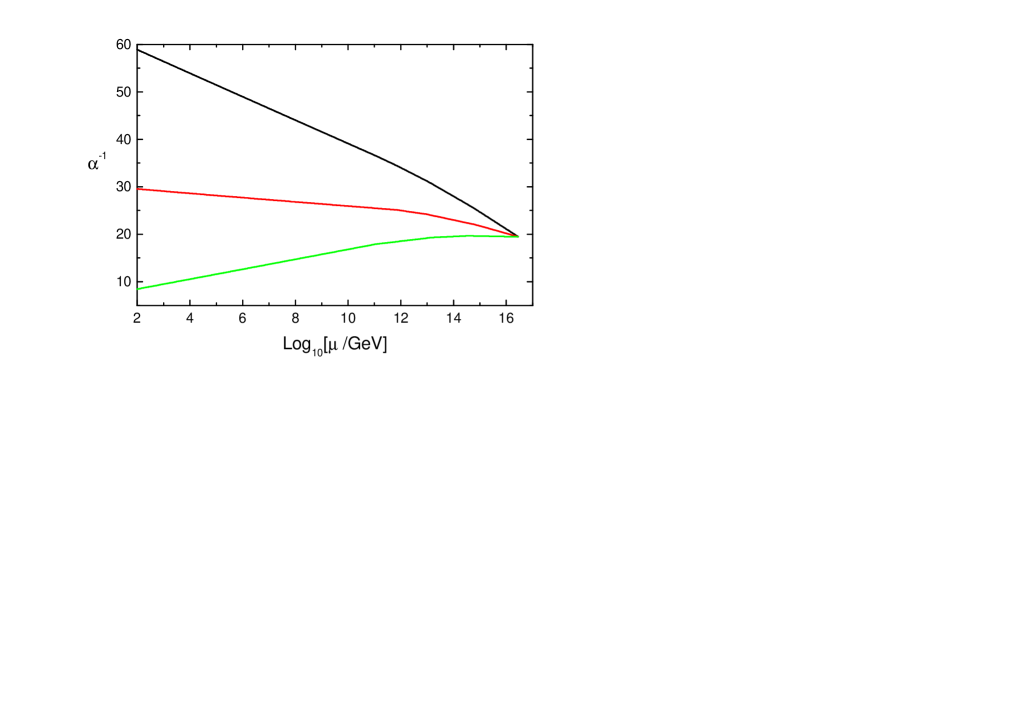
Figure 1: $SU(6)$ Unification with $\alpha_{s}(M_{Z})=0.119$, $M_{G}=2.7\cdot 10^{16}$ GeV and $\alpha_{G}\simeq 1/19.5$.

References

• [1] Particle Data Group, Eur. Phys. J. C 15 (2000) 1.
• [2] P. Langacker, N. Polonsky, Phys. Rev. D 52 (1995) 52; J. Bagger, K. Matchev, D. Pierce, Phys. Lett. B 348 (1995) 443.
• [3] See second ref. of [2] and also I. Gogoladze, hep-ph/9612365; J. Chkareuli, I. Gogoladze, Phys. Rev. D 58 (1998) 055011.
• [4] Q. Shafi, Z. Tavartkiladze, Phys. Lett. B 459 (1999) 563.
• [5] H. Georgi, C. Jarlskog, Phys. Lett. B 88 (1979) 279; J. Harvey, P. Ramond, D. Reiss, Phys. Lett. B 92 (1980) 309; S. Dimopoulos, L.J. Hall, S. Raby, Phys. Rev. Lett. 68 (1992) 1984; V. Barger et. al., Phys. Rev. Lett. 68 (1992) 3394; H. Arason et. al., Phys. Rev. D 47 (1993) 232.
• [6] S. Dimopoulos, F. Wilczek, in Erice Summer Lectures, Plenum, New York, 1981; H. Georgi, Phys. Lett. B108 (1982) 283; B. Grinstein, Nucl. Phys. B206 (1982) 387; A. Masiero el al., Phys. Lett. B115 (1982) 380; J.L. Lopez, D.V. Nanopoulos, Phys. Rev. D53 (1996) 2670.
• [7] S. Dimopoulous, F. Wilczek, NSF-ITP-82-07 (unpublished); M. Srednicki, Nucl. Phys. B202 (1982) 327; K.S. Babu, S.M. Barr, Phys. Rev. D48 (1993) 5354; S.M. Barr, S. Raby, hep-ph/9705366.
• [8] J. Chkareuli, A. Kobakhidze, Phys. Lett. B 407 (1997) 234; J. Chkareuli, I. Gogoladze, A. Kobakhidze, Phys. Rev. Lett. 80 (1988) 912; J. Chkareuli et al., Phys. Rev. D 62 (2000) 015014; Nucl. Phys. B 594 (2001) 23.
• [9] K. Inoue, A. Kakuto, T. Takano, Progr. Theor. Phys. 75 (1986) 664; A. Anselm, A. Johansen, Phys. Lett. B200 (1988) 331; Z. Berezhiani, G. Dvali, Sov. Lebedev Institute Reports 5 (1989) 55.
• [10] R. Barbieri, G. Dvali, A. Strumia, Nucl. Phys. B391 (1993) 487; R. Barbieri, G. Dvali, M. Moretti, Phys. Lett. B312 (1993) 137; R. Barbieri et al., Nucl.Phys. B432 (1994) 49; Z. Berezhiani, Phys. Lett. B355 (1995) 481; Z. Berezhiani, C. Csaki, L. Randall, Nucl. Phys. B444 (1995) 61; G. Dvali, S. Pokorski, Phys. Rev. Lett. 78 (1997) 807; Q. Shafi, Z. Tavartkiladze, Nucl. Phys. B 573 (2000) 40.
• [11] B.Ananthanarayan and Q. Shafi, Phys. Rev. D 54 (1996) 3488.
• [12] G. Dvali, Q. Shafi, Phys. Lett. B 326 (1994) 258; B339 (1994) 241; G. Lazarides, C. Panagiotakopoulos, Q. Shafi, Phys. Lett. B 315 (1993) 325; G. Dvali, Q. Shafi, Phys. Lett. B 403 (1997) 65.
• [13] Q. Shafi, Z. Tavartkiladze, Nucl. Phys. B 552 (1999) 67.
• [14] G. Dvali, Phys. Lett. B 324 (1994) 59; I. Gogoladze, A. Kobakhidze, Z. Tavartkiladze, Phys. Lett. B 372 (1996) 246; A. Kobakhidze, Phys. Lett. B 391 (1997) 335; Z. Tavartkiladze, Phys. Lett. B 392 (1997) 360.
• [15] Q. Shafi, Z. Tavartkiladze, Phys. Lett. B 451 (1999) 129; Phys. Lett. B 482 (2000) 145.
Refer to caption