TUM-HEP-414/01

MPI-PhT/01-13

hep-ph/0105071

Systematic Exploration of the Neutrino Factory Parameter Space
including Errors and Correlations^∗

M. Freund,  P. Huber and  M. Lindner 

^,,Theoretische Physik, Physik Department, Technische Universität München,

James–Franck–Strasse, D–85748 Garching, Germany

Max-Planck-Institut für Physik, Postfach 401212, D–80805 München, Germany

Abstract

We discuss in a systematic way the extraction of neutrino masses, mixing angles and leptonic CP violation at neutrino factories. Compared to previous studies we put a special emphasis on improved statistical methods and on the multidimensional nature of the combined fits of the ${\nu_{e}\rightarrow\nu_{\mu}}$, ${\bar{\nu}_{e}\rightarrow\bar{\nu}_{\mu}}$ appearance and ${\nu_{\mu}\rightarrow\nu_{\mu}}$, ${\bar{\nu}_{\mu}\rightarrow\bar{\nu}_{\mu}}$ disappearance channels. Uncertainties of all involved parameters and statistical errors are included. We find previously ignored correlations in the multidimensional parameter space, leading to modifications in the physics reach, which amount in some cases to one order of magnitude. Including proper statistical errors we determine for all parameters the improved sensitivity limits for various baselines, beam energies, neutrino fluxes and detector masses. Our results allow a comparison of the physics potential for different choices of baseline and beam energy with regard to all involved parameters. In addition we discuss in more detail the problem of parameter degeneracies in measurements of $\delta_{\mathrm{CP}}$.

1 Introduction

The potential to measure neutrino masses, mixings, matter effects and leptonic CP violation at neutrino factories has already been studied for different setups (see e.g. [1, 2, 3]). Among the main points discussed are the achievable precision for the oscillation parameters, the optimal baseline and the best muon energy, the search for matter effects, the search for CP violation and specifically, whether measurements of the CP phase are possible. The results of such studies depend, however, strongly on the chosen experimental setup and the assumed physics parameters, and the combined total parameter space is not easily overlooked.

A common strategy to deal with this situation is to discuss only one or two parameters simultaneously, while the remaining parameters are set to “standard values” (like the muon flux or $\sin^{2}2\theta_{23}=1$). This is a good method for first estimates of the physics capabilities of such experiments. Statistical errors computed in this way are, however, underestimated since they miss possible correlations with the parameters which are hold fixed. This can lead to quite severe errors, especially close to the sensitivity limits, where a strong interplay between several parameters exists. Similar problems arise in a two step analysis, where the disappearance channel is analyzed with sub-leading corrections ignored, and where the extracted leading parameters are used for the extraction of sub-leading parameters.

We present in this work an event rate analysis based on a statistical method, which treats all parameters on equal footing instead of arbitrarily selecting specific parameter subsets. The best method would be to perform full six parameter fits to the simulated event rates, but this is not feasible, since the required computing time for the exploration of the parameter space and the parameter dependencies is enormous. We adopt therefore a somewhat simplified, but still general method which is based on the calculation of all two dimensional slices through the fit manifold. This method is related to the covariance matrix method and it automatically includes all two parameter correlations. We apply this method to the analysis of all involved physics parameters as a function of the machine parameters. In particular, we give improved sensitivity limits for measurements of the mixing angle $\theta_{13}$, matter effects and CP violation. There, the impact of the improved statistical treatment is most evident: Sensitivity limits can be deteriorated by up to one order of magnitude by correlations with sub-leading parameters. We demonstrate furthermore how input from other experiments (like KamLAND [4]) helps to improve the results obtained from neutrino factories. Finally, we study the possibility of combining two distinct baselines and we present results, which help to determine the optimal baseline and the best muon energy.

The paper is organized as follows: First we present in section 2.1 analytic formulae for the relevant oscillation probabilities in vacuum and in matter, which allows to understand many numerical results qualitatively. In section 2.2 we provide a classification scheme of the parameter space, which is important, since it provides an overview of how we analyze and discuss the complex parameter space in detail in section 4. The framework which we use for our numerical simulation of event rates has been discussed in detail in earlier works. We explain this framework therefore only briefly in section 2.3 and we give references to earlier studies. The statistical methods which we used in our study are described in detail in section 3. The results are given in section 4, where we follow the classification scheme introduced in sec. 2.2. Finally, in section 5 we conclude.

2 Framework

2.1 Oscillation probabilities in vacuum and in matter

We assume standard three neutrino mixing with the leptonic mixing matrix $U$, which coincides with the standard parameterization of the quark mixing matrix [5]. The probabilities which describe in vacuum flavour oscillations between an arbitrary number of neutrinos are

$$P_{lm}=\delta_{lm}-4\sum_{k>h}\operatorname{Re}(J^{e_{m}e_{l}}_{kh})\sin^{2}\Delta_{kh}-2\sum_{k>h}\operatorname{Im}(J^{e_{m}e_{l}}_{kh})\sin(2\Delta_{kh})~{},$$ (1)

where $J^{e_{i}e_{j}}_{kh}:=U_{e_{i}\nu_{k}}U_{\nu_{k}e_{j}}^{\dagger}U_{e_{j}\nu_{h}}U_{\nu_{h}e_{i}}^{\dagger}$, $\Delta_{kh}:={\Delta m^{2}_{kh}}L/(4E_{\nu})$ and $\Delta:=\Delta_{31}$. Matter effects lead to sizable corrections of these probabilities. The numerical results shown in section 4 are based on event rates, calculated from the full oscillation formulae, with the matter potential included. As usual, it is assumed that only muons can be detected and a number of the results can be understood analytically from the corresponding probabilities $P({\nu_{\mu}\rightarrow\nu_{\mu}})$ and $P({\nu_{e}\rightarrow\nu_{\mu}})$. The full expressions are, however, quite lengthy and do not allow much insight. We provide therefore simplified expressions by expanding these probabilities in the small mass hierarchy parameter $\alpha:={\Delta m^{2}_{12}}/{\Delta m^{2}_{31}}$. Interesting CP- and ${\Delta m^{2}_{12}}$-effects will only occur for bi-maximal mixing and if $\alpha$ is not too small, i.e. for the LMA-MSW solution of the solar neutrino deficit. We focus therefore on the currently favoured LMA-MSW solution of the solar neutrino deficit [6]. The expansion in $\alpha$ is a good approximation as long as the oscillation governed by the solar ${\Delta m^{2}_{21}}$ is small compared to the leading atmospheric oscillation, i.e.  $\alpha{\Delta}\lesssim 1$. This translates into a upper bound for the baseline:

$$L\lesssim 8000\,\mathrm{km}\left(\frac{E_{\nu}}{\,\mathrm{GeV}}\right)\left(\frac{10^{-4}\,\mathrm{eV}^{2}}{{\Delta m^{2}_{21}}}\right)~{}.$$ (2)

Up to order $\alpha^{2}$ one obtains for the vacuum appearance and disappearance probabilities:

$$P(\nu_{e}\rightarrow\nu_{\mu}) \approx \sin^{2}\theta_{23}\sin^{2}2\theta_{13}\sin^{2}{\Delta}$$ (3)

$$\pm \alpha\;\sin\delta_{\mathrm{CP}}\cos\theta_{13}\sin 2\theta_{12}\sin 2\theta_{13}\sin 2\theta_{23}\sin^{3}{\Delta}$$

$$+ \alpha\;\cos\delta_{\mathrm{CP}}\cos\theta_{13}\sin 2\theta_{12}\sin 2\theta_{13}\sin 2\theta_{23}\cos{\Delta}\sin^{2}{\Delta}$$

$$+ \alpha^{2}\cos^{2}\theta_{23}\sin^{2}2\theta_{12}\sin^{2}{\Delta}$$

$$P(\nu_{\mu}\rightarrow\nu_{\mu}) \approx 1-\cos^{2}\theta_{13}\sin^{2}2\theta_{23}\sin^{2}{\Delta}$$ (4)

$$+ 2\alpha\cos^{2}\theta_{13}\cos^{2}\theta_{12}\sin^{2}2\theta_{23}{\Delta}\cos{\Delta}$$

The numerical magnitude of the different terms in the expansion is affected by different powers of the small mixing angle $\theta_{13}$. All terms of the expansion can be written in the form $\alpha^{n_{\alpha}}\theta_{13}^{n_{\theta}}$ and for $\alpha\simeq\theta_{13}$ the numerical size of each term is roughly controlled by $n=n_{\alpha}+n_{\theta}$. This amounts effectively to a reordering of the expansion in eq. (3), where all terms have $n=2$. Note that all terms proportional to $\alpha$ have also a $\sin 2\theta_{13}$ factor and are thus typically of the same magnitude as the $\alpha^{2}$-term. Higher orders of the expansion in $\alpha$ are, however, always suppressed relative to these leading terms, since $n_{\theta}\geq 0$. The precise magnitude of the terms which are in the sense of this reordering of the same magnitude depends of course on the parameter values, especially on the size of $\alpha$ compared to $\theta_{13}$. For $\theta_{13}$ close to the present upper bound ($\sin^{2}2\theta_{13}\approx 0.1$), the first term of eq. (3) is, for example, dominating and the last term which is proportional to $\alpha^{2}$ is tiny and can be ignored. For smaller values of $\theta_{13}$, all four terms have approximately the same importance and all of them have to be considered for analytical explanations. The last $\alpha^{2}$-term in eq. (3) can only become dominating for extremely tiny values of $\theta_{13}$.

The CP phase $\delta_{\mathrm{CP}}$ produces only in the appearance channel significant effects. This can be seen from eq. (4), where $\delta_{\mathrm{CP}}$ does not show up, while $\delta_{\mathrm{CP}}$ is contained in eq. (3). Both terms in eq. (3), which contain information on the CP phase are, however, suppressed by the mass hierarchy. The precise value of ${\Delta m^{2}_{21}}$ has thus considerable impact on the magnitude of CP-violating effects. There is a profound difference between seeing CP-violating effects directly in an experiment and optimally measuring the CP phase $\delta_{\mathrm{CP}}$ on the other hand. The point is that the term in (eq. 3) which is proportional to $\sin\delta_{\mathrm{CP}}$ changes sign when anti-neutrinos are considered and violates CP explicitely. The CP phase enters, however, also in the term which contains $\cos\delta_{\mathrm{CP}}$, which does not violate CP explicitely, but still can and should be used as an important lever arm to extract $\delta_{\mathrm{CP}}$ from measurements. We treat the CP phase $\delta_{\mathrm{CP}}$ in our analysis therefore exactly in the same way as all other parameters, i.e. we fit rates to the full equations including the $\cos\delta_{\mathrm{CP}}$-term and constrain the parameter space of $\delta_{\mathrm{CP}}$. Our numerical analysis also includes matter effects naturally, and the procedure has therefore the important advantage that it maximally exploits the information on $\delta_{\mathrm{CP}}$ contained in the appearance channels.

For baselines above some hundred kilometers, one must include also the matter potential felt by neutrinos passing through the Earth. This opens the interesting possibility to observe MSW-effects [7, 8, 9, 10] in the appearance channel, while the disappearance probability $P(\nu_{\mu}\rightarrow\nu_{\mu})$ is only marginally affected by matter effects. We include these effects in our numerical analysis and for an analytic discussion we are interested in a reliable and traceable expression for $P(\nu_{e}\rightarrow\nu_{\mu})$ in matter of constant average density. A simple approximative result which is valid for small values of $\theta_{13}$ was derived in [11], where also expressions for larger values of $\theta_{13}$ are given. Similar formulas were also derived in [12, 2].

$$P(\nu_{e}\rightarrow\nu_{\mu}) \approx \sin^{2}\theta_{23}\sin^{2}2\theta_{13}\frac{\sin^{2}[(\hat{A}-1){\Delta}]}{(1-\hat{A})^{2}}$$ (5)

$$\pm \alpha\;\sin\delta_{\mathrm{CP}}\cos\theta_{13}\sin 2\theta_{12}\sin 2\theta_{13}\sin 2\theta_{23}\sin({\Delta})~{}\frac{\sin(\hat{A}{\Delta})}{\hat{A}}\frac{\sin[(1-\hat{A}){\Delta}]}{(1-\hat{A})}$$

$$+ \alpha\;\cos\delta_{\mathrm{CP}}\cos\theta_{13}\sin 2\theta_{12}\sin 2\theta_{13}\sin 2\theta_{23}\cos({\Delta})~{}\frac{\sin(\hat{A}{\Delta})}{\hat{A}}\frac{\sin[(1-\hat{A}){\Delta}]}{(1-\hat{A})}$$

$$+ \alpha^{2}\cos^{2}\theta_{23}\sin^{2}2\theta_{12}\frac{\sin^{2}(\hat{A}{\Delta})}{\hat{A}^{2}}~{}.$$

Here, $\hat{A}=A/{\Delta m^{2}_{31}}=2VE_{\nu}/{\Delta m^{2}_{31}}$ and $V=\sqrt{2}G_{F}n_{e}$ where $G_{F}$ is the Fermi coupling constant and $n_{e}$ the electron density of the involved matter profile. The expressions show at first sight that in the limit of small baselines, the vacuum result (eq. 3) is recovered.

2.2 Classification of oscillation parameters

The full three neutrino oscillation formulae eq. (1) have in general a rather complex parameter structure. All mass splittings and mixing parameters, namely ${\Delta m^{2}_{31}}$, ${\Delta m^{2}_{21}}$, $\theta_{12}$, $\theta_{13}$, $\theta_{23}$ and $\delta_{\mathrm{CP}}$ appear in the relevant transition probabilities even after the expansion in $\alpha$ of section 2.1. The expansion allows, however, to make use of two experimentally justified facts: First, the hierarchy of the neutrino mass splittings, i.e. $\alpha={\Delta m^{2}_{12}}/{\Delta m^{2}_{31}}\ll 1$, which allows to identify hierarchy suppressed “small ${\Delta m^{2}}$ effects”. Second, the mixing angle $\theta_{13}$ is small with $\sin^{2}2\theta_{13}<0.1$ [13], leading to further suppression factors as outlined in section 2.1. The smallness of these two parameters allows to classify the parameter space with the help of the analytic formulae in the scheme below, which is useful for reasons of structure and clarity. Our results are, however, based on a full numerical calculation, which essentially confirm this classification, but also fails in some places, as we will see later in this work.

$\bullet$ Leading parameters:
For ${\Delta m^{2}_{21}}=0$ and $\theta_{13}=0$, there are no transitions in the ${\nu_{e}\rightarrow\nu_{\mu}}$ appearance channel. The disappearance probability reduces to the two neutrino case $P({\nu_{\mu}\rightarrow\nu_{\mu}})=1-\sin^{2}2\theta_{23}\sin^{2}{\Delta}$ being controlled by $\theta_{23}$, ${\Delta m^{2}_{31}}$, which we call leading parameters. These parameters have already been measured by atmospheric neutrino experiments [14, 15, 16] and will be determined better by conventional long baseline experiments [17, 18, 19, 20]. A neutrino factory will allow precision measurements of $\theta_{23}$ and ${\Delta m^{2}_{31}}$ and the result will be limited mainly by systematical errors. The measurement of these parameters will be dominated by the unsuppressed rates in the ${\nu_{\mu}\rightarrow\nu_{\mu}}$ and ${\bar{\nu}_{\mu}\rightarrow\bar{\nu}_{\mu}}$ disappearance channels, which does not rely on excellent charge identification capabilities for secondary muons . The differential event rate distribution allows precise fits of the energy spectrum and the question is only how good $\theta_{23}$ and ${\Delta m^{2}_{31}}$ can be measured for certain detector and neutrino factory parameters, i.e. what the optimal beam energy and baseline are in this context. It will also be interesting to see how the accuracy for the leading parameters is modified for baselines which optimize the sensitivity to $\sin^{2}2\theta_{13}$ or CP violation. This will be addressed in section 4.1.

$\bullet$ Sub-leading parameters:
For $\theta_{13}\neq 0$ and ${\Delta m^{2}_{21}}=0$, the first term in the appearance probabilities eq. (3) or in matter eq. (5) becomes non-zero: $P({\nu_{e}\rightarrow\nu_{\mu}})=\sin^{2}\theta_{23}\sin^{2}2\theta_{13}\sin^{2}((\hat{A}-1){\Delta})/(\hat{A}-1)^{2}$. The appearance channel depends then via $\hat{A}$ on the sign of ${\Delta m^{2}_{31}}$ [2, 3, 21]. In addition to the leading parameters, the analysis depends at this level also on $\theta_{13}$ and $\mathrm{sgn}{\Delta m^{2}_{31}}$, which we call sub-leading parameters. Whether it is possible to determine these sub-leading parameters depends crucially on the value of $\theta_{13}$, and the sensitivity limit below which no effects from $\theta_{13}$ can be measured will be studied in detail. Matter effects have so far not been measured and an experimental test of MSW-effects [7, 8, 9, 10] will be possible if $\theta_{13}$ is large enough. The measurement of $\theta_{13}$ and the search for matter effects [2, 3, 1, 12] are thus important topics for the physics program of a neutrino factory, which do not depend on ${\Delta m^{2}_{21}}$ and $\theta_{12}$ being in the LMA-MSW range. Measurements of rates in the appearance channel depend, however, crucially on the capability to identify the charges of the secondary muons very reliably [3], which requires improved detector technology. Sensitivity limits to $\theta_{13}$ and statistical errors are studied in section 4.2, where also baseline and beam energy optimization are discussed.

$\bullet$ Sub-sub-leading parameters:
Finally, for ${\Delta m^{2}_{21}}\neq 0$ and $\theta_{13}\neq 0$, effects due to the small solar mass squared splitting are added and the remaining three parameters appear in the oscillation formulae: ${\Delta m^{2}_{21}}$, $\theta_{12}$ and the CP phase $\delta_{\mathrm{CP}}$. Measuring leptonic CP violation is an exciting possibility for neutrino factories. In order to obtain sufficient rates, this requires, however, that the LMA-MSW region is the correct solution to the solar neutrino problem. One can see immediately from eq. (3) that ${\Delta m^{2}_{21}}$ (i.e. $\alpha$) and $\theta_{13}$ are the crucial parameters with determine the absolute and relative strength of the CP-violating effects. The foreseeable experiments are often not too far from the sensitivity limit. The limits on those two parameters, which will be discussed in section 4.3, are therefore among the most important points of this study, providing a better understanding how to search for CP violation and how $\delta_{\mathrm{CP}}$ can be extracted. We will also see in section 4.3 that $\theta_{12}$ and ${\Delta m^{2}_{21}}$ can be measured only very poorly in neutrino factory experiments. To a good approximation only the product ${\Delta m^{2}_{21}}\sin 2\theta_{21}$ can be determined, which can be expected already from the the appearance probability in eq. (3). Thus we expect and will see that ${\Delta m^{2}_{21}}$ and $\theta_{12}$ are highly correlated. Results obtained from neutrino factories cannot compete with results expected from the long baseline reactor experiment KamLAND [22]. It is thus very important to study how external input on ${\Delta m^{2}_{21}}$ and $\theta_{12}$ (e.g. from KamLAND) helps to improve the extraction of CP-violating effects at a neutrino factory. The related questions about the optimal baseline and beam energy will be discussed in detail. As already mentioned above, the effects from the CP phase $\delta_{\mathrm{CP}}$ are, like the matter effects, best accessible in the appearance channels ${\nu_{e}\rightarrow\nu_{\mu}}$ and ${\bar{\nu}_{e}\rightarrow\bar{\nu}_{\mu}}$ which rely strongly on excellent charge identification capabilities of the detector.

Note that the extraction of both the sub-leading and sub-sub-leading parameters is essentially based on moderate event rates, which can be estimated from the oscillation probability at a mean energy. Unlike the disappearance channels, there is thus essentially no information in the energy spectrum. Note also that the above classification in leading, sub-leading and sub-sub-leading effects is also useful from a practical point of view. The experimental abilities of a neutrino factory will realistically develop from an initial, low flux setup, which is able to measure the leading parameters only, to a high luminosity machine, capable of measuring sub-leading and probably sub-sub-leading effects. This will allow in a good approximation an extraction of parameters at the relevant level, where the remaining parameters of the level below act essentially as unknown variables.

2.3 Event rate analysis of neutrino factory experiments

Our numerical analysis (see ref. [3] for details) is based on simulated event rates, which are calculated using neutrino flux profiles, full three neutrino oscillation probabilities in matter, a realistic Earth matter profile, neutrino cross sections, detector mass, threshold and energy resolution. Backgrounds and experimental uncertainties are not taken into account. The $\nu_{e}-$, $\bar{\nu}_{e}-$, $\nu_{\mu}-$ and $\bar{\nu}_{\mu}-$fluxes produced by a symmetrically operated neutrino factory of given muon energy and polarization can easily be derived from the muon flux and the kinematics of muon decay. The transition probabilities are calculated numerically by propagating the neutrino states through a realistic Earth density profile. The resulting muon event rates are then computed by folding the neutrino flux, the transition probabilities and the cross sections with the energy resolution function of the detector. The assumed muon detection threshold is $4\,\mathrm{GeV}$. The energy resolution of the detector is approximated by a Gaussian resolution function with $\sigma=0.1E$, which gives an energy resolution $\Delta E/E=10\%$. This value resembles the energy resolution of MONOLITH [23] for $\nu_{\mu}$ charged current events.

With this method, event rates are calculated for the ${\nu_{e}\rightarrow\nu_{\mu}}$, ${\bar{\nu}_{e}\rightarrow\bar{\nu}_{\mu}}$ appearance and ${\nu_{\mu}\rightarrow\nu_{\mu}}$, ${\bar{\nu}_{\mu}\rightarrow\bar{\nu}_{\mu}}$ disappearance transitions with 20 energy bins in each channel. We assume perfect muon charge separation, i.e. that the different appearance and disappearance channels can be well separated. This requires for the appearance channels excellent charge identification capabilities of the detector. Insufficient charge identification would reduce the physics reach of such an experiment as pointed out in [3]. The type of detector assumed for this study is a magnetized iron detector with a mass of 10 kt. With $2\cdot 10^{20}$ muon decays per year we obtain a standard “luminosity” of $N_{\mu}\,m_{\mathrm{kt}}=2\cdot 10^{21}\,\mathrm{kt}\,\mathrm{year}$. We consider, however, also variations of the parameter $N_{\mu}\,m_{\mathrm{kt}}$. Thus, different fluxes like an initial $10^{19}$ muon decays per year or higher fluxes (or detector masses) are considered. The details of the statistical analysis are explained in chapter 3. The analysis uses simultaneously the neutrino and anti-neutrino channels of both the disappearance and appearance rate vectors, leading in all cases to optimal results. The method works of course also in cases where the results are dominated by one channel. Note, that $N_{\mu}$ is the sum of muons of both polarities, which means that the parameter $N_{\mu}\,m_{\mathrm{kt}}$ normalizes the sum of the neutrino and the anti-neutrino channels. Further details of the simulations can be found in ref. [3].

3 Statistical methods

There are a number of non-trivial aspects in neutrino factory studies which require suitable statistical methods. We describe therefore in this section in more detail the problems and the methods used in this work. We also compare our method with other previously used methods.

The aim of the analysis is to obtain statistically reliable statements about possible measurements of ${\Delta m^{2}_{21}},\,{\Delta m^{2}_{31}},\,\theta_{12},\,\theta_{13},\,\theta_{23}$ and $\delta_{\mathrm{CP}}$. A numerical scan of the full six dimensional input parameter with a subsequent extraction of the input parameters is an enormous numerical task. Therefore, up to now most studies performed only two parameter fits to evaluate the physics reach of a neutrino factory [12, 3, 24, 21, 25, 26, 27, 28, 1]. Often two parameters of the full parameter set, which were thought to be most relevant, were selected and a fit to this two parameters was performed using a $\chi^{2}$-method. All other parameters were at the same time fixed to their best fit (i.e. input) values. Typically Gauss or Poisson $\chi^{2}$-functions have been used, i.e.

$$\mathrm{Gauss}\quad\chi^{2} = \sum_{i=1}^{b}\frac{(x_{i}-\langle x_{i}\rangle)^{2}}{\sigma_{i}^{2}}\thinspace,$$ (6)

$$\mathrm{Poisson}\quad\chi^{2} = \sum_{i=1}^{b}\left(2[\langle x_{i}\rangle-x_{i}]+2\thinspace x_{i}\log\frac{x_{i}}{\langle x_{i}\rangle}\right)\thinspace,$$ (7)

where $b$ denotes the number of bins, $x_{i}$ is the number of events in bin $i$ and $\langle x_{i}\rangle$ denotes the expectation value for bin $i$. $\sigma_{i}$ is estimated by $\sqrt{x_{i}}$. This method is numerically straightforward, but it is not easy to include uncertainties of the left out parameters and systematical errors. The Gaussian $\chi^{2}$-function allows, however, an approximate treatment of such uncertainties by Gaussian error propagation:

$$\chi^{2} = \sum_{ij}(x_{i}-\langle x_{i}\rangle)\,V^{-1}_{ij}\,(x_{j}-\langle x_{j}\rangle)\thinspace,$$ (8)

$$V_{ij} = \sigma_{i}^{2}\delta_{ii}+\sum_{\alpha=1}^{n}\frac{\partial\langle x_{i}\rangle}{\partial\lambda_{\alpha}}\,\frac{\partial\langle x_{j}\rangle}{\partial\lambda_{\alpha}}\,\sigma_{\alpha}^{2}\thinspace.$$

Here $\lambda_{\alpha}$ is one out of $n$ (in our case $n=6$) parameters and $\sigma_{\alpha}$ denotes the uncertainty of $\lambda_{\alpha}$. This method was for example used in [29]. It is, however, important to keep in mind that such an approach relies on the validity of the linear approximation of the functional dependence of $\langle x_{i}\rangle$ on $\lambda$. The point is that Gaussian error propagation relies only on the linear terms of a Taylor expansion of $\langle x_{i}\rangle$ in $\lambda$. The above approach may thus be no longer justified as soon as the second or higher order terms become important.

Using one of eqs. 6-8, the acceptance region $M$ at confidence level $\alpha$ is given by:

$$\chi^{2}(\hat{\lambda}) \leq \chi^{2}(\lambda)\quad\forall\lambda\thinspace,$$ (9)

$$\Delta\chi^{2}(\lambda) := \chi^{2}(\lambda)-\chi^{2}(\hat{\lambda})\thinspace,$$

$$M = \{\lambda:\Delta\chi^{2}(\lambda)\leq\Delta\chi^{2}_{\alpha}\}\thinspace.$$ (10)

Using the asymptotic properties of maximum likelihood estimators, $\Delta\chi^{2}_{\alpha}$ is determined from the condition that the area under a $\chi^{2}$-distribution from zero to $\Delta\chi^{2}_{\alpha}$ equals $\alpha$. The number of degrees of freedom for this distribution is given by the number of free parameters $r$ in the fit. The error on the confidence level $\alpha$ is then given by the size of the $r$-dimensional manifold $M$. This procedure leads to an error interval $I_{\lambda_{i}}$ for each of the $r$ fitted parameters by simply projecting $M$ onto $\lambda_{i}$. We define the infimum and supremum with respect to $\lambda_{i}$, i.e. the lower (upper) bound on $\lambda_{i}$:

$$\inf_{\lambda_{i}}(M) := \inf(\{\lambda_{i}:\lambda\in M\})\thinspace,$$

$$\sup_{\lambda_{i}}(M) := \sup(\{\lambda_{i}:\lambda\in M\})\thinspace.$$ (11)

$I_{\lambda_{i}}$ is then given by:

$$I_{\lambda_{i}}=\left[\inf_{\lambda_{i}}(M),\sup_{\lambda_{i}}(M)\right]\thinspace.$$ (12)

This method leads for $n=2$ and a Gaussian likelihood to the usual error ellipses.

We use a method which we call the Generalized Covariance Matrix Method (gcmm), where $\chi^{2}$ is calculated according to eq. 7 with $n=6$ parameters, namely $\lambda=({\Delta m^{2}_{21}},{\Delta m^{2}_{31}},$ $\theta_{12},\theta_{13},\theta_{23},\delta_{\mathrm{CP}})$. The computational effort required to calculate the full six-dimensional manifold $M$ is enormous. To reduce this effort we adopted a scheme, which takes all 2-parameter-correlations into account. We calculate therefore all two dimensional slices $S_{ij}$ of $M$ through $\hat{\lambda}$ which are parallel to the coordinate planes in order to estimate the errors for all six parameters:

$$P_{ij} = \{\lambda:\lambda_{k}\equiv\hat{\lambda}_{k};k\not=i,j\}\thinspace,$$

$$S_{ij} = \{\lambda\in P_{ij}:\Delta\chi^{2}(\lambda)\leq\Delta\chi^{2}_{\alpha}\}\thinspace.$$ (13)

These slices can be seen in the upper row of fig. 1, where the method is graphically explained.

Figure 1: Illustration of the error determination for a single parameter (in this example $\sin^{2}2\theta_{13}$). In the upper row $\sin^{2}2\theta_{13}$ is fitted against the remaining 5 other parameters (grey regions) and the individual error bars of our method for each parameter are overlayed. These error bars result from the projection of the grey regions onto $\sin^{2}2\theta_{13}$. All these errors are then combined into a total error for $\sin^{2}2\theta_{13}$, given by the lowest and highest endpoints of the individual errors. The result is shown as a grey region in the lower row, where the individual errors are overlayed.

There are five such slices for one parameter and the largest extension of the projection of these five slices down to the parameter of interest is the corresponding error of this parameter. The error interval $I_{\lambda_{i}}$ of a parameter $\lambda_{i}$ is thus given by

$$I_{\lambda_{i}} = \bigcup_{k\not=i}\left[\inf_{\lambda_{i}}(S_{ik}),\sup_{\lambda_{i}}(S_{ik})\right]\thinspace,$$ (14)

which corresponds to the grey band in the lower row of fig. 1. We use for $\Delta\chi^{2}_{\alpha}$ the value $9.2$ which corresponds to 99% C.L. for two degrees of freedom, and to 83.8% C.L. for six degrees of freedom. The big advantage of the gcmm method is that no choice about “most influential” parameters has to be made. Instead, the method automatically finds the most influential parameters, like in the example of fig. 1, where the biggest error for $\theta_{13}$ surprisingly comes from ${\Delta m^{2}_{21}}$. Previous neutrino factory studies used so far only one of the $S_{ij}$ to estimate the accuracy to which parameters can be extracted. We will show in this work that this can be a poor approximation, since some of the parameters, like $\theta_{13}$ and ${\Delta m^{2}_{21}}$, are strongly correlated in a previously overlooked way. We will see that the sensitivity to $\sin^{2}2\theta_{13}$ can be reduced in this way up to one order of magnitude. Another advantage of the gcmm method is, that it can cope with uncertainties of all parameters even if the parameter dependence is highly non-linear, as it is often the case in neutrino oscillation studies. The gcmm method is thus in a number of ways better than a Gaussian error propagation. The gcmm is, however, still only an approximation, and full six parameter fits will lead to corrections. We compared the gcmm method to three parameter fits and found that it works quite good, but the difference can in the worst case amount to a factor of two.

A final aspect of the analysis concerns the inclusion of parameters from other experiments. This leads to an understanding of how the parameter improvements of other experiments affect the analysis. An important case is ${\Delta m^{2}_{21}}$, which can be measured by KamLAND [22] in the LMA-MSW case with a precision which is much better than what can be obtained at a neutrino factory, as will be discussed in detail in section 4.3. It is therefore important to perform an analysis, where such external information can be included and where its impact can be assessed. Usually we extract in our analysis parameters by finding their best fit value and by determining the errors with the fitting procedure to our “data”. In order to include external knowledge of some parameter (e.g. on ${\Delta m^{2}_{21}}$), we simply restrict the range of variation of the is parameter in the fits to the error interval at confidence level $\alpha$.

For the CP-phase there will, however, exist no information in advance. Since $\delta_{\mathrm{CP}}$ determines which correlations are important, the errors on specific parameters can significantly depend on the value of $\delta_{\mathrm{CP}}$. In such cases, the analysis is done for all possible values of $\delta_{\mathrm{CP}}$ and the maximal error which appears is taken as the final error. We call this procedure “$\delta_{\mathrm{CP}}$ unknown”. It is equivalent to integrating out a nuisance parameter with uniform prior in a Bayesian analysis.

4 Results

The results obtained from the numerical study are presented following the outline given in sec. 2.2. First, the leading parameters $\theta_{23}$ and ${\Delta m^{2}_{31}}$ are discussed in sec. 4.1. Then, measurements of $\theta_{13}$, matter effects and the sign of ${\Delta m^{2}_{31}}$ are studied in sec. 4.2. Finally, CP-violating effects and measurements of ${\Delta m^{2}_{21}}$ and $\theta_{12}$ are presented in sec. 4.3. The reader can select certain topics without missing information which is necessary for the understanding since the contents of these sections widely do not depend on each other.

4.1 Leading parameters $\theta_{23}$ and ${\Delta m^{2}_{31}}$

First, we will discuss the statistical sensitivity to the leading parameters $\theta_{23}$ and ${\Delta m^{2}_{31}}$. Neutrino factory experiments will allow high precision measurements of these two parameters, which are at present only roughly determined. The information on these parameters dominantly stems from disappearance channel measurements. Thus, the dependence on the value of $\theta_{13}$ is marginal, especially when $\theta_{13}$ is small. It will be demonstrated that the influence from uncertainties on ${\Delta m^{2}_{21}}$ and $\theta_{21}$ can however be substantial. This has the consequence that input from other experiments (like KamLAND) can be helpful to limit the errors of the affected measurements.

Optimization of baseline $L$ and muon energy $E_{\mu}$

Figure 2: Statistical (relative) error of ${\Delta m^{2}_{31}}$ (left plot) and $\sin^{2}2\theta_{23}$ (right plot) as function of the baseline $L$ and the muon energy $E_{\mu}$ for ${\Delta m^{2}_{31}}=3.5\cdot 10^{-3}\,\mathrm{eV}^{2}$, $\sin^{2}2\theta_{23}=1$ and $N_{\mu}\,m_{\mathrm{kt}}=2\cdot 10^{21}\,\mathrm{kt}\,\mathrm{year}$. Dark shading indicates the preferred regions. For $\delta({\Delta m^{2}_{31}})$, the best sensitivity reached is $\delta_{\mathrm{min}}=7.7\%$. For $\delta({\Delta m^{2}_{31}})$ it is $6.1\%$. The contour lines indicate factors of 2, 5 and 10 accuracy loss compared to the best values. The sub-leading parameters $\sin^{2}2\theta_{13}$, ${\Delta m^{2}_{21}}$ and $\delta_{\mathrm{CP}}$ do not play a crucial role and are assumed as unknown (see sec. 3).

Fig. 2 shows the expected statistical error on the quantities ${\Delta m^{2}_{31}}$ and $\sin^{2}2\theta_{23}$ in dependence of the neutrino factory parameters, baseline $L$ and muon energy $E_{\mu}$ at $N_{\mu}\,m_{\mathrm{kt}}=2\cdot 10^{21}\,\mathrm{kt}\,\mathrm{year}$. For beam energies above $20\,\mathrm{GeV}$ and baselines above $2000\,$km, the statistical error on ${\Delta m^{2}_{31}}$ takes values between roughly $8\%$ and $16\%$. For not too small muon energies, the important constraint is the baseline limit. The above mentioned $2000\,$km define the limit where the accuracy loss relative to the best value is less then a factor of two. This baseline limit linearly depends on the inverse of ${\Delta m^{2}_{31}}$, which was chosen to be $3.5\cdot 10^{-3}\,\mathrm{eV}^{2}$ in the above case. For ${\Delta m^{2}_{31}}=1.0\cdot 10^{-3}\,\mathrm{eV}^{2}$ the limit shifts to approximately $5000\,$km above which the statistical error is less than 20%. For ${\Delta m^{2}_{31}}=6.5\cdot 10^{-3}\,\mathrm{eV}^{2}$ the limit is well below $1000\,$km and the statistical error does not exceed 14%.

The statistical error in measurements of the mixing angle $\theta_{23}$ (right plot of fig. 2) is, with minimally 6%, at the same level of the one on ${\Delta m^{2}_{31}}$. Also here, a baseline limit can be given under which the statistical error is larger than twice the best achievable value. For ${\Delta m^{2}_{31}}=3.5\cdot 10^{-3}\,\mathrm{eV}^{2}(1.0\cdot 10^{-3}\,\mathrm{eV}^{2})$ this limit is roughly $3000\,$km ($5000\,$km). The figure indicates that there is a favored value of $L/E_{\mu}$, which can easily be understood using analytic considerations: Information on $\theta_{23}$ is dominantly extracted from the total rates observed in the disappearance channel $P(\nu_{\mu}\rightarrow\nu_{\mu})$ which is is not significantly affected by matter effects. Assuming a discrete neutrino energy corresponding to the average neutrino energy in the disappearance channel ($\left<E_{\nu}\right>=16/21E_{\mu}$), the number of observed muon neutrino events is approximately given by $N=(1-\sin^{2}2\theta_{23}\sin^{2}\hat{\Delta}_{31})\Phi_{\nu_{\mu}}$, where the factor $\Phi_{\nu_{\mu}}$ includes flux, cross-sections and detector mass. For $N_{\mu}\,m_{\mathrm{kt}}=2\cdot 10^{21}\,\mathrm{kt}\,\mathrm{year}$, we find that $\Phi_{\nu_{\mu}}=6.910^{6}(L/\mathrm{km})^{-2}(16/21E_{\mu}/\,\mathrm{GeV}^{2})^{3}$. In the Gaussian limit, which is a good approximation here, the relative statistical error on the quantity $\sin^{2}2\theta_{23}$ is given by

$$\left|\frac{\Delta\sin^{2}2\theta_{23}}{\sin^{2}2\theta_{23}}\right|=\frac{1}{\sqrt{\Phi_{\nu_{\mu}}}}\frac{\sqrt{1-\sin^{2}2\theta_{23}\sin^{2}\hat{\Delta}_{31}}}{\sin^{2}2\theta_{23}\sin^{2}\hat{\Delta}_{31}}=f(\frac{L}{E_{\mu}})E_{\mu}^{-1/2}~{}.$$ (15)

Thus, the relative error on $\sin^{2}2\theta_{23}$ is approximately a function of $L/E_{\mu}$ with a slight modification from the factor $E_{\mu}^{-1/2}$. For muon energies between $10\,\mathrm{GeV}$ and $50\,\mathrm{GeV}$ this modification maximally gives a correction of $(50/10)^{-1/2}\approx 0.45$ which in general reduces the error for higher muon energies. The corresponding plot in fig. 2 clearly shows the contour lines of constant $L/E_{\mu}$. Using eq. 15 with the parameters corresponding to fig. 2 yields a relative error for $\sin^{2}2\theta_{23}$ at the level 1/1000. For the quantity $\theta_{23}$ this translates to a relative error at the level of some per cent, which is in good agreement with the results obtained in the full numerical analysis.

Summarily, the leading parameters do not give very strong recommendations for the selection of the baseline and muon energy. Beam energies between $30\,\mathrm{GeV}$ and $50\,\mathrm{GeV}$ are recommended. To achieve a sufficiently developed oscillation, the baseline must be large enough. For the central value of ${\Delta m^{2}_{31}}$ proposed by the Super-Kamiokande experiment, a baseline of $3000\,$km or more would be suitable. Should it turn out in the future, that ${\Delta m^{2}_{31}}$ is at the lower edge of the presently favored region, one should be aware that this baseline limit shifts to higher values roughly inverse proportionally to ${\Delta m^{2}_{31}}$. The exact values of the sub-leading parameters $\theta_{13}$ and $\delta_{\mathrm{CP}}$ do not play a role in this discussion since the results presented here depend only weakly on them. But ${\Delta m^{2}_{21}}$ being correlated with ${\Delta m^{2}_{31}}$ can have some impact on the errors made in measurements of ${\Delta m^{2}_{31}}$. This point will be discussed in detail later.

Dependance on flux and detector mass $N_{\mu}\,m_{\mathrm{kt}}$

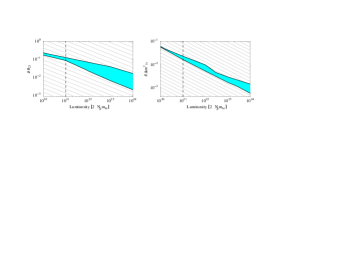
Figure 3: Statistical error of $\theta_{23}$ (left plot) and ${\Delta m^{2}_{31}}$ (right plot) as function of $N_{\mu}\,m_{\mathrm{kt}}$, the number of stored muons per year times the mass of the neutrino detector in kilotons. The shaded bands indicate the range which is covered by variations of the sub-leadingparameters $\theta_{13}$ and ${\Delta m^{2}_{21}}$ ($0\leq\sin^{2}2\theta_{13}\leq 10^{-1}$, $10^{-5}\leq{\Delta m^{2}_{21}}\leq 10^{-4}$). The calculation of $\delta(\theta_{23})$ was performed with $50\,\mathrm{GeV}$ muon energy and a baseline of $7000\,$km ($\delta\theta_{23}$) respectively $3000\,$km ($\delta{\Delta m^{2}_{31}}$).

The influence of $N_{\mu}\,m_{\mathrm{kt}}$, the number of stored muons per year times the mass of the neutrino detector in kilotons, is shown in fig. 3. The decrease of the statistical error with increasing $N_{\mu}\,m_{\mathrm{kt}}$ roughly follows the prediction from Gaussian statistics ($1/\sqrt{N_{\mu}\,m_{\mathrm{kt}}}$), which is indicated by the parallel lines in the background of the figure. The spread of the shaded band is generated by variations of the sub-leading parameters. Their influence increases with higher luminosities where the statistical errors are small.

Correlation between ${\Delta m^{2}_{31}}$ and ${\Delta m^{2}_{21}}$

It is important to note that, for specific selections of $L$ and $E_{\mu}$, the statistical error on ${\Delta m^{2}_{31}}$ is dominated by its correlation with ${\Delta m^{2}_{21}}$. This fact is displayed in fig. 4, which shows the results of two parameter fits of ${\Delta m^{2}_{31}}$ with all other oscillation parameters. The plot shows that the dominating contribution to the statistical error of ${\Delta m^{2}_{31}}$ stems from the uncertainties of ${\Delta m^{2}_{21}}$ and $\theta_{12}$. This suggests that in such cases, external information on ${\Delta m^{2}_{21}}$ and $\theta_{12}$ from other experiments can considerably improve the precision of measurements of ${\Delta m^{2}_{31}}$.

Figure 4: Error bars of all two parameter fits which include ${\Delta m^{2}_{31}}$. The total error (grey shaded region) is dominated by the contributions from the fits against ${\Delta m^{2}_{21}}$ and $\theta_{12}$. Fitting ${\Delta m^{2}_{31}}$ only against $\theta_{23}$ can result in a considerable underestimation of $\delta({\Delta m^{2}_{31}})$. The calculation was performed with $L=8000\,$km, $E_{\mu}=50\,\mathrm{GeV}$, $\theta_{12}=\pi/4$, $\sin^{2}2\theta_{13}=10^{-3}$, ${\Delta m^{2}_{21}}=10^{-4}\,\mathrm{eV}^{2}$ and $N_{\mu}\,m_{\mathrm{kt}}=2\cdot 10^{21}\,\mathrm{kt}\,\mathrm{year}$.

With fig. 5, this point is investigated in more detail: There, the resulting statistical error on ${\Delta m^{2}_{31}}$ is given as function of $\delta({\Delta m^{2}_{21}})$, the error on ${\Delta m^{2}_{21}}$ as provided from external measurements. The shaded band indicates the expected values of $\delta({\Delta m^{2}_{21}})$ from measurements performed at the KamLAND experiment [22]. The plots show that KamLAND input can improve the statistical error on ${\Delta m^{2}_{31}}$ up to a factor of three. This, however, is only valid for specific baselines. At smaller baselines this correlation is not very pronounced.

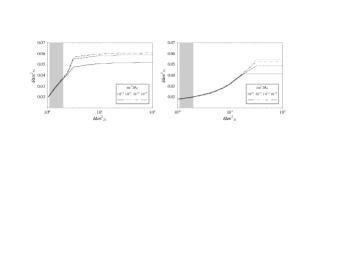
Figure 5: Statistical error on ${\Delta m^{2}_{31}}$ as function of $\delta({\Delta m^{2}_{21}})$, the error on ${\Delta m^{2}_{21}}$ as provided from external measurements (like the KamLAND experiment). The shaded band indicates the expected values of $\delta({\Delta m^{2}_{21}})$ from measurements performed at the KamLAND experiment [22]. No external input corresponds to the right edge of the plot ($\delta({\Delta m^{2}_{21}})=10^{2}$). The calculation was done for ${\Delta m^{2}_{21}}=10^{-4}\,\mathrm{eV}^{2}$ (left panel) respectively for ${\Delta m^{2}_{21}}=10^{-5}\,\mathrm{eV}^{2}$ (right panel) and $\theta_{12}=\pi/4$. The different line styles indicate different values of $\sin^{2}2\theta_{13}$ ($10^{-4}$, $10^{-3}$, $10^{-2}$, $10^{-1}$).

4.2 Sub-leading parameters $\theta_{13}$ and $\mathrm{sgn}{\Delta m^{2}_{31}}$

Following the outline given in section 2.2, we continue this study with a discussion of the parameter $\theta_{13}$. Information on $\theta_{13}$ is mainly obtained from the appearance channel probabilities $P(\nu_{e}\rightarrow\nu_{\mu})$ and $P(\bar{\nu}_{e}\rightarrow\bar{\nu}_{\mu})$, which contain terms proportional to $\sin 2\theta_{13}$ and $\sin^{2}2\theta_{13}$. For not too small values of $\sin^{2}2\theta_{13}$, the results presented in this section are roughly independent from the sub-sub-leading parameters ${\Delta m^{2}_{21}}$, $\theta_{12}$ and $\delta_{\mathrm{CP}}$. In this case, a neutrino factory experiment will be able to measure $\theta_{13}$ with some precision. However, for small values of $\sin^{2}2\theta_{13}$ close to the sensitivity reach, the parameters ${\Delta m^{2}_{21}}$, $\theta_{12}$ and $\delta_{\mathrm{CP}}$ can have considerable impact on measurements of $\theta_{13}$. This is an example where the step-wise analysis of such experiments is no longer valid.

Optimization of baseline $L$ and muon energy $E_{\mu}$

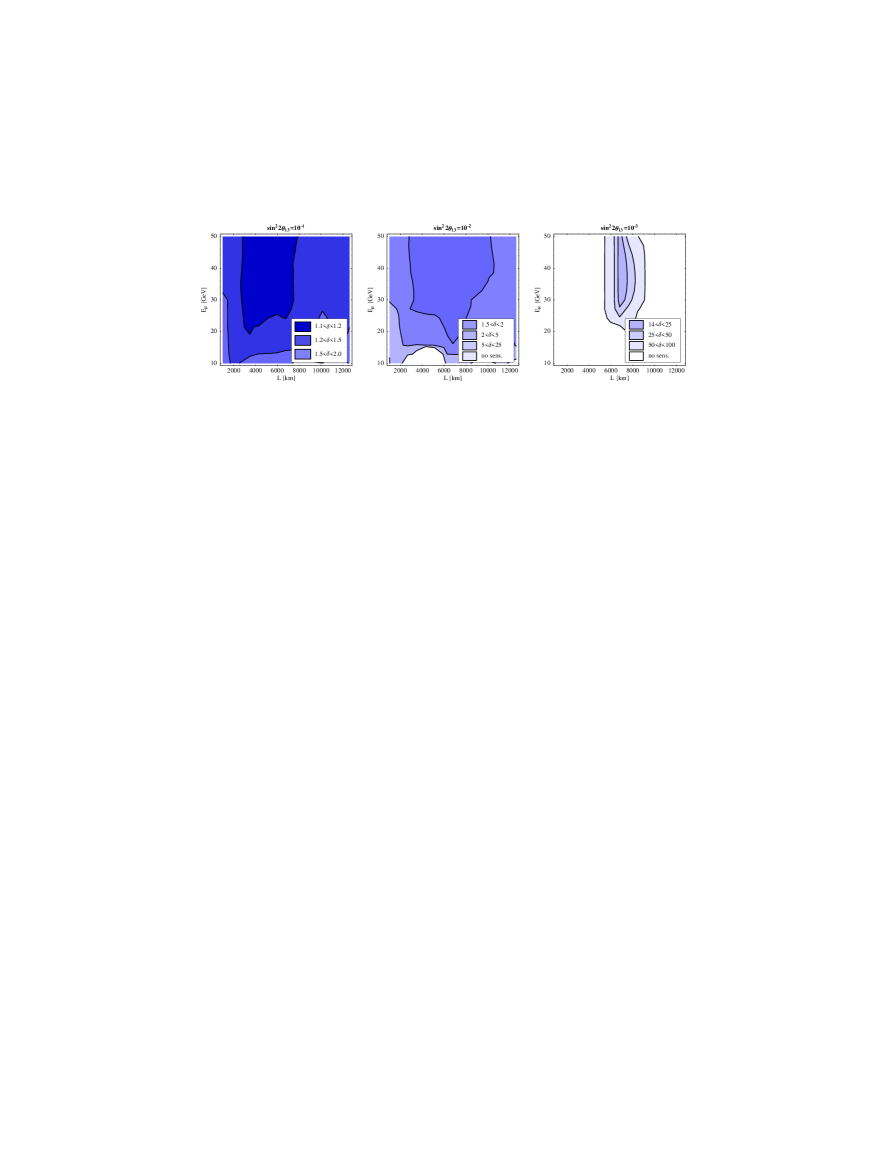
Figure 6: Statistical error of the quantity $\sin^{2}2\theta_{13}$ as function of the baseline $L$ and the muon energy $E_{\mu}$ for ${\Delta m^{2}_{31}}=3.5\cdot 10^{-3}\,\mathrm{eV}^{2}$, $\sin^{2}2\theta_{23}=1$, $N_{\mu}\,m_{\mathrm{kt}}=2\cdot 10^{21}\,\mathrm{kt}\,\mathrm{year}$ and three values of $\sin^{2}2\theta_{13}$ ($10^{-1}$, $10^{-2}$, $10^{-3}$). Dark shading indicates the preferred regions. The parameters ${\Delta m^{2}_{21}}$ and $\delta_{\mathrm{CP}}$ play a role mainly for small values of $\theta_{13}$. Here, they are assumed as unknown (see sec. 3).

$\sin^{2}2\theta_{13}$	$10^{-1}$	$10^{-2}$	$10^{-3}$	$10^{-4}$
${\Delta m^{2}_{31}}=6.0\cdot 10^{-3}\,\mathrm{eV}^{2}$	1.1	1.2	2.1	10
${\Delta m^{2}_{31}}=3.5\cdot 10^{-3}\,\mathrm{eV}^{2}$	1.1	1.5	14	–
${\Delta m^{2}_{31}}=1.0\cdot 10^{-3}\,\mathrm{eV}^{2}$	3.3	180	–	–

Table 1: Statistical errors $\delta$ made in measurements of $\sin^{2}2\theta_{13}$ listed for several values of ${\Delta m^{2}_{31}}$. The quantity $\delta$, whose values are given in the table is the same as in fig. 6. A detailed description of $\delta$ is given in the text.

The statistical error of $\sin^{2}2\theta_{13}$ in dependence of the neutrino factory parameters baseline $L$ and beam energy $E_{\mu}$ is displayed in fig. 6. The plotted quantity is

$$\delta:=\mathrm{max}\{(z_{\mathrm{min}}/z_{0})^{-1},z_{\mathrm{max}}/z_{0}\}~{},$$ (16)

where $z=\sin^{2}2\theta_{13}$ and the subscripts correspond to the central value (0), the minimal value (min) and the maximal value (max) which are compatible with the simulated experimental data. For values of $\delta$ close to 1, $\delta-1$ is approximately equal to the relative error. $\delta=10(100)$ indicates one (two) order(s) of magnitude uncertainty on the measured quantity. Since the error strongly depends on the value $\sin^{2}2\theta_{13}$, three plots for the values $\sin^{2}2\theta_{13}=(10^{-1},10^{-2},10^{-3})$ are given. For $\sin^{2}2\theta_{13}=10^{-1}$ (left plot), the sensitivity is good and reaches values between 10% and 20% relative error at baselines between $3000\,$km and $8000\,$km and with beam energies above $20\,\mathrm{GeV}$. For $\sin^{2}2\theta_{13}=10^{-2}$ (middle plot), still errors down to 50% are reachable. Close to the sensitivity reach $\sin^{2}2\theta_{13}=10^{-3}$ (right plot), the situation is interesting. There, the information is still sufficient to determine $\sin^{2}2\theta_{13}$ with an error corresponding to roughly one order of magnitude. But now, close to the sensitivity limit, long baselines between $7000\,$km and $8000\,$km are strongly preferable. The reason for this is, that for small values of $\sin^{2}2\theta_{13}$, the correlations of $\theta_{13}$ with ${\Delta m^{2}_{21}}$ and $\delta_{\mathrm{CP}}$ are important. These correlations tend to have less influence at large baselines. Since previous studies concerning the optimization of the baseline [12] did not include these correlations, they missed this point and came to differing recommendations for the baseline. Note, that close to the sensitivity limit, the result depends strongly on the precise value of the CP phase $\delta_{\mathrm{CP}}$. For the calculation which is presented here, we assume that $\delta_{\mathrm{CP}}$ is completely unknown: The statistical errors are computed for several values of $\delta_{\mathrm{CP}}$ and the maximal error of this set is considered as the final result.

In table 1 the statistical errors made in measurements of $\sin^{2}2\theta_{13}$ are listed for several values of ${\Delta m^{2}_{31}}$. The value of ${\Delta m^{2}_{31}}$ changes the obtained results significantly. Higher values of ${\Delta m^{2}_{31}}$ increase the precision, whereas lower values make it more difficult to measure $\theta_{13}$.

Correlation between $\theta_{13}$ and the sub-sub-leading parameters ${\Delta m^{2}_{21}}$ and $\delta_{\mathrm{CP}}$

In connection with measurements of $\delta_{\mathrm{CP}}$ it has been recognized that the correlation of the CP phase $\delta_{\mathrm{CP}}$ with the mixing angle $\theta_{13}$ could possibly hide the effect of CP violation [29]. The implications of this correlation on the expected precision of measurements of of $\theta_{13}$ have not been discussed. Already in the baseline discussion above, it was shown that in case of small values of $\theta_{13}$, correlations with $\delta_{\mathrm{CP}}$ and ${\Delta m^{2}_{21}}$ can drastically influence the statistical errors expected in measurements of $\sin^{2}2\theta_{13}$.

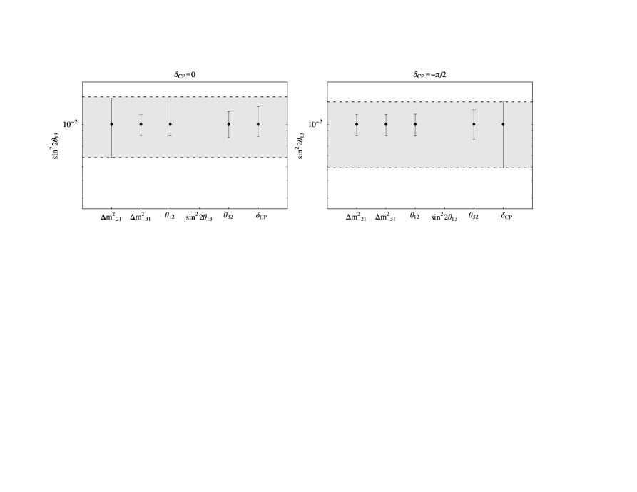
Figure 7: Error bars of all two parameter fits which include $\sin^{2}2\theta_{13}$ for $\delta_{\mathrm{CP}}=0$ (left plot) and $\delta_{\mathrm{CP}}=\pi/2$ (right plot). The total error (grey shaded region) is dominated by the contributions from the fits against ${\Delta m^{2}_{21}}$ (left plot) or $\delta_{\mathrm{CP}}$ (right plot). Fitting $\sin^{2}2\theta_{13}$ only together with ${\Delta m^{2}_{31}}$ can result in a considerable underestimation of the statistical error. The calculation was performed with $L=2100\,$km, $E_{\mu}=50\,\mathrm{GeV}$, $\theta_{12}=\pi/4$, $\sin^{2}2\theta_{13}=10^{-2}$, ${\Delta m^{2}_{21}}=10^{-4}\,\mathrm{eV}^{2}$ and $N_{\mu}\,m_{\mathrm{kt}}=2\cdot 10^{21}\,\mathrm{kt}\,\mathrm{year}$.

To illustrate this, fig. 7 shows the results of two parameter fits of $\sin^{2}2\theta_{13}$ with all other oscillation parameters for two different values of the CP phase $\delta_{\mathrm{CP}}$. The plots demonstrate that the dominating contribution to the statistical error of $\sin^{2}2\theta_{13}$ can be caused by correlations with the parameters ${\Delta m^{2}_{21}}$ or $\delta_{\mathrm{CP}}$. In the case $\delta_{\mathrm{CP}}=0$ (left plot), the main error stems from the correlation with ${\Delta m^{2}_{21}}$ but for $\delta_{\mathrm{CP}}=\pi/2$ (right plot), it is the CP phase $\delta_{\mathrm{CP}}$ which gives the dominating contribution to the total error. The correlation with ${\Delta m^{2}_{21}}$ severely affects the sensitivity to $\sin^{2}2\theta_{13}$ which was completely overlooked up to now.

The influence of the sub-sub-leading parameters ${\Delta m^{2}_{21}}$ and $\delta_{\mathrm{CP}}$ for the measurement of $\theta_{13}$ can qualitatively be understood using analytic considerations. For small values of $\theta_{13}$ at the sensitivity limit, all four terms of equation 5 are equally important. The first, leading term has always a positive sign. The second term $\propto\alpha\,\sin\delta_{\mathrm{CP}}\,\sin^{2}2\theta_{13}$ has a sign which depends on $\delta_{\mathrm{CP}}$ and whether neutrinos or anti-neutrinos are considered. Since we always use neutrinos and anti-neutrinos, this term can have both signs. The sign of the third term $\propto\alpha\,\cos\delta_{\mathrm{CP}}\,\sin^{2}2\theta_{13}$ is determined by the value of $\delta_{\mathrm{CP}}$. The sign of the fourth term $\propto\alpha^{2}$ is always positive. If $\cos\delta_{\mathrm{CP}}<0$ an increase (decrease) in $\theta_{13}$ can be compensated by an increase (decrease) in ${\Delta m^{2}_{21}}$. In this case the main problem arises from the correlation of $\theta_{13}$ and $\delta_{\mathrm{CP}}$, since all terms containing $\delta_{\mathrm{CP}}$ are proportional to ${\Delta m^{2}_{21}}\sin^{2}2\theta_{13}$ and this product can not be determined very well. Also the event rates are considerably smaller in this case which simply leads to a loss of statistical significance especially close to the sensitivity limit. If $\cos\delta_{\mathrm{CP}}>0$ an increase (decrease) in $\theta_{13}$ can be compensated by a decrease (increase) in ${\Delta m^{2}_{21}}$, therefore the product ${\Delta m^{2}_{21}}\sin^{2}2\theta_{13}$ can be determined quite accurately. In this case where the correlation of $\sin^{2}2\theta_{13}$ with ${\Delta m^{2}_{21}}$ causes the problems, external information on ${\Delta m^{2}_{21}}$ (e.g. from KamLAND) would help to improve the results.

It is also possible to understand, why large baselines around $7000\,$km are recommended in case of low values of $\theta_{13}$ and large values of ${\Delta m^{2}_{21}}$: The relative size of the terms containing $\delta_{\mathrm{CP}}$ decreases with growing baseline. Thus in principle larger baselines should perform better. For too long baselines, the $1/L^{2}$-decrease of event rates starts to worsen the result again. The numerical calculation shows that baselines around $7000\,\mathrm{km}$ perform by far best. Shorter baselines can profit considerably from external input on ${\Delta m^{2}_{21}}$ if (and only if) $\cos\delta_{\mathrm{CP}}>0$.

It is of great importance to recognize that for small values of $\theta_{13}$ and large values of ${\Delta m^{2}_{21}}$ the contributions to the total error of measurements of $\theta_{13}$, originating from the sub-sub-leading sector, are substantial and not only minor corrections. With decreasing ${\Delta m^{2}_{21}}$, these contributions get smaller and in the limit ${\Delta m^{2}_{21}}=0$ there is no influence left from the parameters ${\Delta m^{2}_{21}}$, $\theta_{12}$ and $\delta_{\mathrm{CP}}$. The same is true for small values of $\theta_{12}$ (SMA solution).

Sensitivity reach for measurements of $\theta_{13}$

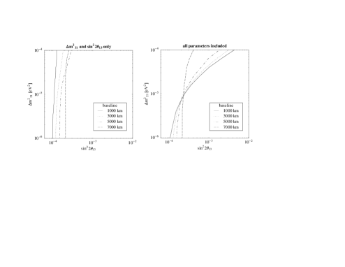
Figure 8: Sensitivity reach for measurements of $\sin^{2}2\theta_{13}$. The area to the left of the lines indicates the parameter range where measurements are compatible with $\sin^{2}2\theta_{13}=0$ at 99% C.L. . The calculation was performed with a beam energy of $50\,\mathrm{GeV}$. The different line types are for different baseline as explained in the legend. For comparison to older studies, the left panel displays the result obtained from a two parameter fit of only $\sin^{2}2\theta_{13}$ and ${\Delta m^{2}_{31}}$. The right panel displays our new result with all parameters taken into account.

We define the “sensitivity reach” for measurements of the mixing angle $\theta_{13}$ as the maximal value of $\sin^{2}2\theta_{13}$ at which the experimental data is compatible with the hypothesis $\sin^{2}2\theta_{13}=0$ at 99% C.L. . Measurements of nonzero values for $\theta_{13}$ are only possible above the sensitivity reach. The sensitivity reach as function of ${\Delta m^{2}_{21}}$ is given by the right hand plot in fig. 8. The different line types indicate different baselines. For very small ${\Delta m^{2}_{21}}$, values down to $\sin^{2}2\theta_{13}\simeq 10^{-4}$ are reachable and baselines between $1000\,\mathrm{km}$ and $7000\,\mathrm{km}$ perform very similar. The sensitivity limit varies only within a factor two. With increasing ${\Delta m^{2}_{21}}$, the effects from the parameters ${\Delta m^{2}_{21}}$ and $\delta_{\mathrm{CP}}$ become stronger and the sensitivity reach deteriorates by more than one order of magnitude (for short baselines). The left hand plot shows the results obtained by a two parameter fit to only $\theta_{13}$ and ${\Delta m^{2}_{31}}$. Since there, the correlation with ${\Delta m^{2}_{21}}$ and $\delta_{\mathrm{CP}}$ are not taken into account and $\delta_{\mathrm{CP}}$ is fixed to zero, the performance of an experiment is nearly independent of ${\Delta m^{2}_{21}}$. Comparing the two plots, it is obvious that with this method, for large values of ${\Delta m^{2}_{21}}$, the performance would be strongly overestimated, especially for baselines below $7000\,\mathrm{km}$. This result is important since it suggests to use a longer baseline for measurements of $\theta_{13}$ than usually proposed.

The dependence of the $\theta_{13}$ sensitivity reach on the parameter $N_{\mu}\,m_{\mathrm{kt}}$ is shown in fig. 9. The scaling behavior is nearly Gaussian, i.e. it is roughly proportional to $\sqrt{N_{\mu}\,m_{\mathrm{kt}}}^{-1}$. At high luminosities systematical errors, like insufficient charge identification capabilities of the detector, will most probably limit the sensitivity.

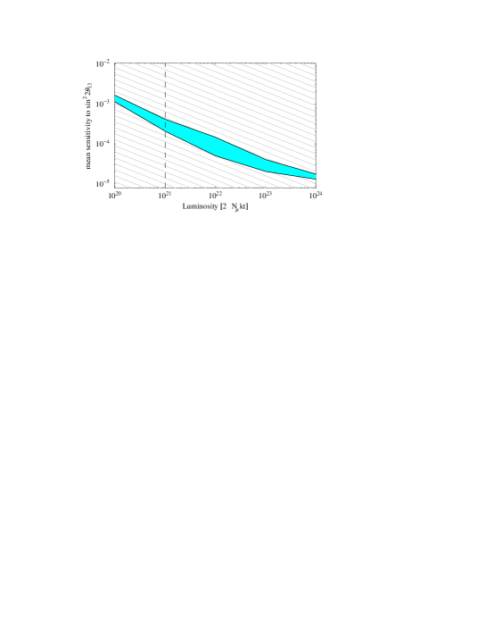
Figure 9: Sensitivity reach (see text for detailed definition) for measurements of $\sin^{2}2\theta_{13}$ as function of $N_{\mu}\,m_{\mathrm{kt}}$, the number of stored muons per year times the mass of the neutrino detector in kilotons. The band indicates the range which is covered by variations of the sub-leadingparameters ${\Delta m^{2}_{21}}$ and $\delta_{\mathrm{CP}}$ ($10^{-5}\leq{\Delta m^{2}_{21}}\leq 10^{-4}$, $-\pi<\delta_{\mathrm{CP}}<\pi$). The calculation was performed with a baseline of $7000\,$km and $50\,\mathrm{GeV}$ muon energy. The vertical dashed line indicates a typical neutrino factory experiment with a 10 kt iron detector.

Sensitivity reach for the determination of $\mathrm{sgn}\,{\Delta m^{2}_{31}}$

The ability to determine the sign of ${\Delta m^{2}_{31}}$ stems from the fact that the MSW-resonance occurs – depending on the sign of ${\Delta m^{2}_{31}}$ – either in the neutrino or in the anti-neutrino appearance channel. Therefore it is very important to be sensitive to the energy region around the MSW-resonance. In references [2, 3, 28] it was shown that, in the case this sensitivity is good, the ability to determine the sign of ${\Delta m^{2}_{31}}$ nearly coincides with the ability to determine $\theta_{13}$. This holds in some approximation also when all parameters are taken into account. Hence, we do not study this point in detail but refer to fig. 9, which should give also a rough idea about the limit on $\theta_{13}$ above which a determination of $\mathrm{sgn}\,{\Delta m^{2}_{31}}$ should be possible. Each term of eq. 5 is invariant under a simultaneous change from neutrino to anti-neutrino and of the sign of ${\Delta m^{2}_{31}}$. Therefore changing the sign of ${\Delta m^{2}_{31}}$ is equivalent to interchanging the role of neutrinos and anti-neutrinos. Assuming symmetric operation of the neutrino factory, the only difference that remains is due to the cross sections, which are for neutrinos twice as large as for anti-neutrinos. In case of a negative sign of ${\Delta m^{2}_{31}}$ one thus looses half of the statistics, which can be compensated by doubling the flux of $\bar{\nu}_{e}$.

4.3 Sub-sub-leading parameters $\theta_{12}$, ${\Delta m^{2}_{21}}$ and $\delta_{\mathrm{CP}}$

Whether it is possible to measure the parameters $\theta_{12}$, ${\Delta m^{2}_{21}}$ and $\delta_{\mathrm{CP}}$ with a neutrino factory long baseline experiment crucially depends on the values of $\theta_{13}$, $\theta_{12}$ and ${\Delta m^{2}_{21}}$. To significantly influence the measured event rates, it is absolutely necessary that the LMA-MSW solution is the correct description for solar neutrino oscillations. In comparison to the results presented in the previous section, which do only depend on the value of $\theta_{13}$, this is a severe additional condition which enables or disables the search for the CP-violating phase $\delta_{\mathrm{CP}}$. Assuming now that the LMA-MSW solution is realized, it is important to notice that the sub-sub-leading effects are proportional to ${\Delta m^{2}_{21}}$, which in the LMA-range can still vary between roughly $2\cdot 10^{-5}\,\mathrm{eV}^{2}$ and $2\cdot 10^{-4}\,\mathrm{eV}^{2}$ (at 99% confidence level)[6]. This means, that the magnitude of CP-violating effects can also vary by one order of magnitude.

In this section we will discuss the following points in detail: First, we will study the precision of measurements of the parameters $\theta_{12}$ and ${\Delta m^{2}_{21}}$ in comparison to the KamLAND experiment. We will show, that the neutrino factory is mainly capable to measure the product ${\Delta m^{2}_{21}}\sin 2\theta_{12}$ but has severe difficulties to constrain ${\Delta m^{2}_{21}}$ and $\theta_{12}$ separately. KamLAND will provide much better accuracy for these parameters. Then, we will focus on the search for CP violation. We will discuss, for different neutrino factory fluxes and detector masses, the magnitude of the effects from the CP phase $\delta_{\mathrm{CP}}$ in dependence of the parameters $\theta_{13}$ and ${\Delta m^{2}_{21}}$. Which baselines and beam energies are best suitable for measurements of the CP phase is also studied in detail. Finally, some specific topics like the parameter degeneracy in the $\theta_{13}$-$\delta_{\mathrm{CP}}$ parameter plane are discussed.

Correlation between $\theta_{12}$ and ${\Delta m^{2}_{21}}$

For ${\Delta m^{2}_{21}}<10^{-4}\,\mathrm{eV}^{2}$, the appearance channel probabilities depend only on the product ${\Delta m^{2}_{21}}\sin 2\theta_{12}$ (see eq. 5). Thus a strong correlation between $\theta_{12}$ and ${\Delta m^{2}_{21}}$ can be expected. The upper plot of fig. 10 shows the result of a two parameter fit

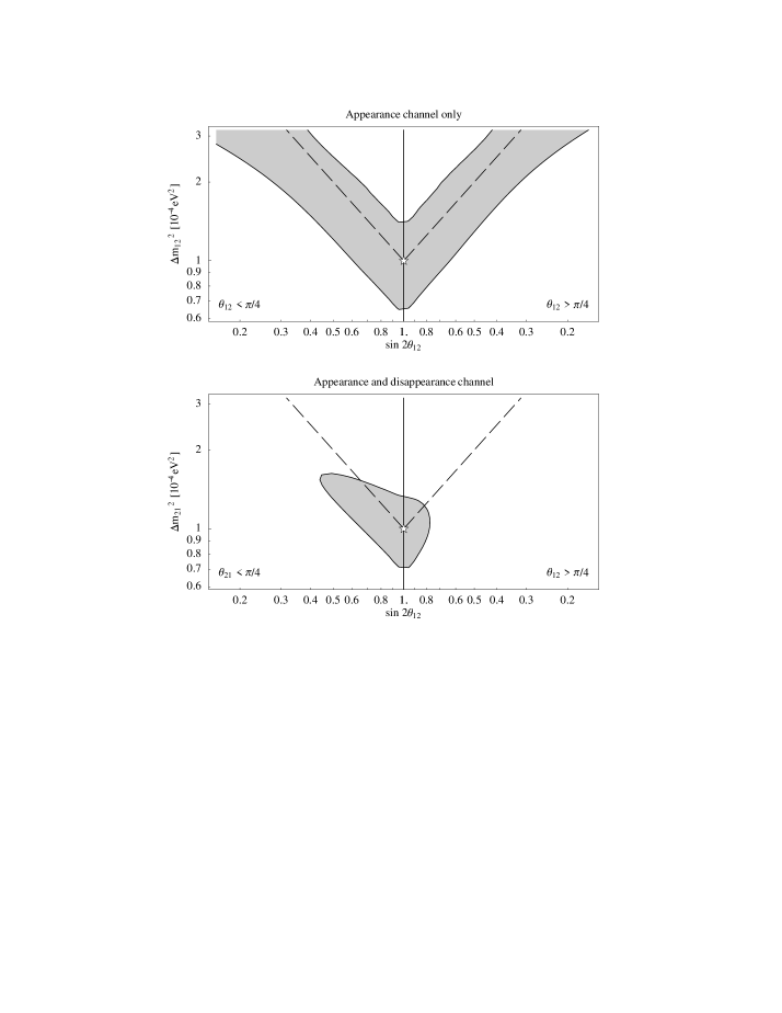
Figure 10: $3\sigma$ contour line of two parameter fits of $\theta_{12}$ and ${\Delta m^{2}_{21}}$ to simulated event rates from the appearance channel only (upper plot) and appearance channel plus disappearance channel (lower plot). Constant values of the product ${\Delta m^{2}_{21}}\sin 2\theta_{12}$ are given by the dashed lines. The calculation was performed with $50\,\,\mathrm{GeV}$ muon energy, $3000\,$km baseline, $N_{\mu}\,m_{\mathrm{kt}}=2\cdot 10^{21}~{}\,\mathrm{kt}\,\mathrm{year}$, $\theta_{12}=\pi/4$, ${\Delta m^{2}_{21}}=10^{-4}\,\mathrm{eV}^{2}$, $\sin^{2}2\theta_{13}=10^{-3}$ (upper plot) and $\sin^{2}2\theta_{13}=10^{-1}$ (lower plot).

of $\theta_{21}$ and ${\Delta m^{2}_{21}}$ to only the appearance rates. From the comparison to the dashed line, which represents the constant value ${\Delta m^{2}_{21}}\sin 2\theta_{12}=10^{-4}\,\mathrm{eV}^{2}$, it can clearly be seen that indeed the measurement is only sensitive to the product ${\Delta m^{2}_{21}}\sin 2\theta_{12}$. For large values of ${\Delta m^{2}_{21}}$, this correlation can be lifted by inclusion of disappearance rates (see lower plot of fig. 10). The sub-leading term in the disappearance probability (eq. 4) depends on the product ${\Delta m^{2}_{21}}\cos^{2}\theta_{12}$, which helps to lift the degeneracy between ${\Delta m^{2}_{21}}$ and $\theta_{12}$. If, however, ${\Delta m^{2}_{21}}$ is small, the $\alpha^{2}$-term in the disappearance probability looses in strength and it gets very difficult to obtain information on $\theta_{12}$ and ${\Delta m^{2}_{21}}$ separately.

Hence, the precision of measurements of $\theta_{12}$ and ${\Delta m^{2}_{21}}$ is in general not very good. Particularly, the performance of a neutrino factory in such measurements is not comparable to the KamLAND experiment. Fig. 11 shows results of two parameter fits of $\theta_{12}$ and ${\Delta m^{2}_{21}}$ from the combined rates of the appearance and disappearance channels for several values of ${\Delta m^{2}_{21}}$ and $\theta_{12}$. The simulated experiment was performed with a luminosity of $N_{\mu}\,m_{\mathrm{kt}}=2\cdot 10^{22}~{}\,\mathrm{kt}\,\mathrm{year}$, which is by a factor ten higher than the standard value used in this work. It can be seen that despite the relatively high value of $N_{\mu}\,m_{\mathrm{kt}}$, the results are not good. Particularly, the error ellipses grow drastically with decreasing $\theta_{12}$ and ${\Delta m^{2}_{21}}$.

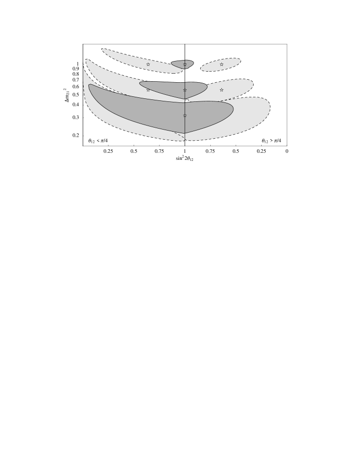
Figure 11: Two parameter fits of $\theta_{12}$ and ${\Delta m^{2}_{21}}$ to combined simulated event rates of the appearance channel and the disappearance channel. The calculation was performed with $50\,\mathrm{GeV}$ muon energy, $3000\,$km baseline, $N_{\mu}\,m_{\mathrm{kt}}=2\cdot 10^{22}~{}\,\mathrm{kt}\,\mathrm{year}$ (!!) and $\sin^{2}2\theta_{13}=10^{-1}$.

Correlation of $\delta_{\mathrm{CP}}$ with $\theta_{13}$ and possible degeneracies

In section 4.2 it was demonstrated that the parameters $\theta_{13}$ and $\delta_{\mathrm{CP}}$ can be strongly correlated. This effect was visualized in the right plot of fig. 7. It is obviously important for studies of the CP-phase $\delta_{\mathrm{CP}}$ and it is discussed in detail in ref. [29]. Since our statistical method takes into account all possible two parameter correlations, also this particular correlation is automatically included in our results. We do not further discuss this correlation but focus on another interesting problem which is also studied in the above referred work.

Figure 12: Fits to $\sin^{2}2\theta_{13}$ and $\delta_{\mathrm{CP}}$ with different values of the energy resolution of the detector (left plot) and $\chi^{2}$–difference between the best fit points of the two degenerate solutions as function of the energy resolution (right plot) . The black square in the right plot denotes the standard energy resolution used in this work. Parameters: $E_{\mu}=50\,\mathrm{GeV}$, $L=3000\,\mathrm{km}$, ${\Delta m^{2}_{21}}=10^{-4}\thinspace\mathrm{eV}^{2}$.

There, it is demonstrated that considering the full parameter space of $\delta_{\mathrm{CP}}$, multiple degenerate solutions appear in simultaneous fits of $\delta_{\mathrm{CP}}$ and $\theta_{13}$. It is also stated that this degeneracy could possibly be lifted when different baselines or beam energies are studied simultaneously. We find that the appearance of degenerate solutions crucially depends on the energy resolution of the detector. In fig. 12 the influence of the energy resolution on a fit of $\delta_{\mathrm{CP}}$ versus $\sin^{2}2\theta_{13}$ is shown. In the left hand plot the fit itself is depicted for the three energy resolutions 10%, 30% and 50%. The second degenerate solution in the upper part of the plot diminishes with increasing resolution and completely vanishes for the value 10%. To further illustrate this effect, the right hand plot shows the $\chi^{2}$-difference of the best fit points of the two degenerate solutions as function of the energy resolution of the detector. The dashed horizontal lines in the plot indicate which energy resolution is needed to refuse the second degenerate solution at a certain confidence level. With an energy resolution of 10%, like we use it throughout this study, the second solution disappears with a confidence of more than 99%. We checked that this holds for all values of $\delta_{\mathrm{CP}}$ and $\theta_{13}$. In ref. [29] the analysis was performed with only five energy bins. This corresponds to an energy resolution, which is too bad to allow a lift of the degeneracy.

Optimization of baseline $L$ and muon energy $E_{\mu}$

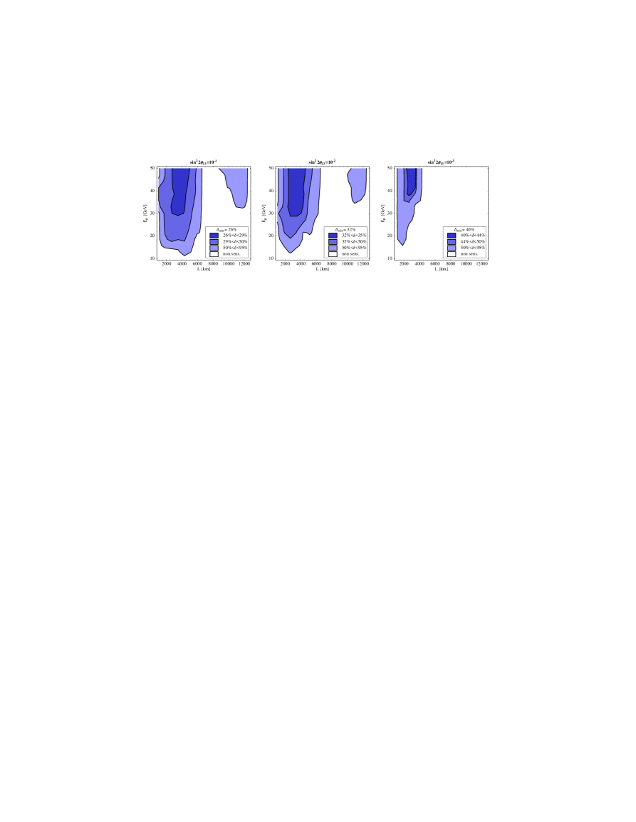
Figure 13: Results of fits of the CP phase $\delta_{\mathrm{CP}}$ as function of the baseline $L$ and the muon energy $E_{\mu}$ for ${\Delta m^{2}_{31}}=3.5\cdot 10^{-3}\,\mathrm{eV}^{2}$, ${\Delta m^{2}_{21}}=10^{-4}\,\mathrm{eV}^{2}$, $\theta_{23}=\pi/4$, $\theta_{12}=\pi/4$, $N_{\mu}\,m_{\mathrm{kt}}=2\cdot 10^{21}\,\mathrm{kt}\,\mathrm{year}$ and three values of $\sin^{2}2\theta_{13}$ ($10^{-1}$, $10^{-2}$, $10^{-3}$). Dark shading indicates the preferred regions. The quantity $\delta$ plotted here is the percentage of the $\delta_{\mathrm{CP}}$ parameter space $[-\pi/2,\pi/2]$ which is compatible with the simulated experimental data at the $3\sigma$ confidence level. The contour lines correspond to $\delta=50\%$ and $\delta=95\%$. In the white shaded region no information on the CP phase can be obtained.

In fig. 13 the regions in $L$-$E_{\mu}$-plane are shown where $\delta_{\mathrm{CP}}$ can be measured. We find that in general higher energies and baselines around $3000\,\mathrm{km}$ are preferred which is in good agreement with the results obtained in [12, 29] but is in clear contradiction to the results obtained in [30, 31]. The reason for this disagreement seems to lie in the different use of statistics. In the referred work no fits are performed but Gaussian error propagation is used (see sec. 3). In table 2 the optimal regions in the $L$-$E_{\mu}$-plane are given for different values of $\sin^{2}2\theta_{13}$.

${\Delta m^{2}_{31}}$	$\sin^{2}2\theta_{13}$	baseline	beam energy
	$10^{-1}$	$2400\,\mathrm{km}\lesssim L\lesssim 4200\,\mathrm{km}$	$E_{\mu}\gtrsim 40\,\mathrm{GeV}$
$6.0\cdot 10^{-3}\,\mathrm{eV}^{2}$	$10^{-2}$	$2400\,\mathrm{km}\lesssim L\lesssim 4000\,\mathrm{km}$	$E_{\mu}\gtrsim 40\,\mathrm{GeV}$
	$10^{-3}$	$1800\,\mathrm{km}\lesssim L\lesssim 2700\,\mathrm{km}$	$E_{\mu}\gtrsim 45\,\mathrm{GeV}$
	$10^{-1}$	$2800\,\mathrm{km}\lesssim L\lesssim 4500\,\mathrm{km}$	$E_{\mu}\gtrsim 30\,\mathrm{GeV}$
$3.5\cdot 10^{-3}\,\mathrm{eV}^{2}$	$10^{-2}$	$2500\,\mathrm{km}\lesssim L\lesssim 4500\,\mathrm{km}$	$E_{\mu}\gtrsim 30\,\mathrm{GeV}$
	$10^{-3}$	$2500\,\mathrm{km}\lesssim L\lesssim 3500\,\mathrm{km}$	$E_{\mu}\gtrsim 40\,\mathrm{GeV}$
	$10^{-1}$	no sens.	no sens.
$1.0\cdot 10^{-3}\,\mathrm{eV}^{2}$	$10^{-2}$	no sens.	no sens.
	$10^{-3}$	no sens.	no sens.

Table 2: Optimal choice of the baseline $L$ and the beam energy $E_{\mu}$ for measurements of the CP phase $\delta_{\mathrm{CP}}$. The data of the first three lines are taken from figs. 13. The given ranges identify the regions where the statistical error $\delta(\delta_{\mathrm{CP}})$ is not more than by a factor 1.1 larger than the optimal value $\delta(\delta_{\mathrm{CP}})_{\mathrm{min}}$. In figs. 13 these regions are indicated by the darkest shading.

We also checked the influence of the value of ${\Delta m^{2}_{31}}$ on the sensitivity and the optimal regions in the $L$-$E_{\mu}$-plane (see table 3 ). The sensitivity gets better (worse) as ${\Delta m^{2}_{31}}$ increases (decreases). The optimal baseline seems to be quite stable against changes of ${\Delta m^{2}_{31}}$. The optimal energy however gets smaller as ${\Delta m^{2}_{31}}$ gets smaller.

${\Delta m^{2}_{31}}$	$\sin^{2}2\theta_{13}$	fraction
	$10^{-1}$	22%
$6.0\cdot 10^{-3}\,\mathrm{eV}^{2}$	$10^{-2}$	24%
	$10^{-3}$	28%
	$10^{-1}$	26%
$3.5\cdot 10^{-3}\,\mathrm{eV}^{2}$	$10^{-2}$	32%
	$10^{-3}$	40%
	$10^{-1}$	100%
$1.0\cdot 10^{-3}\,\mathrm{eV}^{2}$	$10^{-2}$	100%
	$10^{-3}$	100%

Table 3: Fraction of the parameter space of $\delta_{\mathrm{CP}}$ which is covered by the $3\sigma$ acceptance region. 100% means that no information on the CP phase can be extracted from the experimental data. The values are based on ${\Delta m^{2}_{21}}=10^{-4}\,\mathrm{eV}^{2}$, $\theta_{23}=\pi/4$, $\theta_{12}=\pi/4$ and $N_{\mu}\,m_{\mathrm{kt}}=2\cdot 10^{21}\,\mathrm{kt}\,\mathrm{year}$.

Sensitivity reach for $\delta_{\mathrm{CP}}$

The two parameters ${\Delta m^{2}_{21}}$ and $\theta_{13}$ control the size of all CP-effects. A very important question thus is, down to which values of these two parameters the CP phase can be determined.

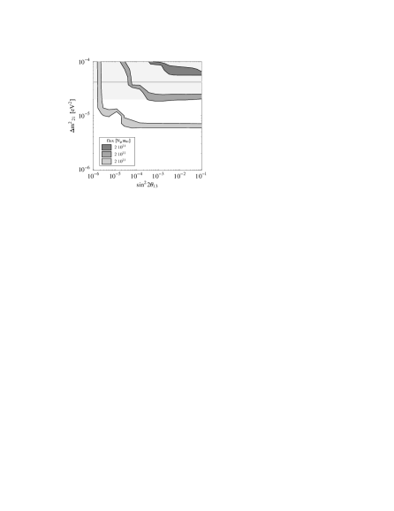
Figure 14: Sensitivity limit of measurements of the CP-phase $\delta_{\mathrm{CP}}$ in the $\theta_{13}$-${\Delta m^{2}_{21}}$ parameter plane for three different values of $N_{\mu}\,m_{\mathrm{kt}}$. The lower edge of each band represents the sensitivity limit under which no information on the CP-phase can be extracted from the experimental data. The upper edges of each band indicates 50% statistical error (at 99% C.L.) for measurements of $\delta_{\mathrm{CP}}$. This result was obtained with a baseline of $3000\,\mathrm{km}$. The light grey shaded region in the background indicates the values of ${\Delta m^{2}_{21}}$ compatible with the LMA-MSW solution and the grey horizontal line indicates its best fit value.

This sensitivity reach is shown in fig. 14. The three grey bands were obtained with luminosities $N_{\mu}\,m_{\mathrm{kt}}$ of $2\cdot 10^{21}\,\mathrm{kt}\,\mathrm{year}$ (dark grey), $2\cdot 10^{22}\,\mathrm{kt}\,\mathrm{year}$ (grey) and $2\cdot 10^{23}\,\mathrm{kt}\,\mathrm{year}$ (light grey). The upper edge of each band represents 50% error, which is the contour line where half of the parameter space of $\delta_{\mathrm{CP}}$ can be ruled out by the experiment. The lower edge represents the sensitivity limit under which no information on $\delta_{\mathrm{CP}}$ can be extracted from the experimental data. The light grey shaded area in the background indicates the presently allowed LMA-MSW solution and the grey horizontal line its best fit value[6]. Note that the so called “initial stage” option $2\cdot 10^{20}\,\mathrm{kt}\,\mathrm{year}$ is not included in the plot since it does not provide sufficient event rates to make the CP-effects accessible. With the standard luminosity assumed in this work ($2\cdot 10^{21}\,\mathrm{kt}\,\mathrm{year}$), CP-effects are only accessible for values of ${\Delta m^{2}_{21}}$ at the upper edge of the LMA-solution. If ${\Delta m^{2}_{21}}$ is at the lower edge, the luminosity must be increased by a factor of more than 10. In this case, however, systematic errors could become the dominant source of uncertainties.

5 Conclusion

Previous neutrino factory studies were based on simplified treatments, which do not include all parameter correlations. We show that these correlations have considerable influence on the physics potential of a neutrino factory, especially for measurements close to the sensitivity limit of $\theta_{13}$ and for measurements of CP violation. We developed for our analysis improved statistical methods which are based on the computation of all two parameter correlations and which automatically include all parameter uncertainties. We used this method to look for all possible correlations and to refine in this way the understanding of the potential of neutrino factories. Using this method we found indeed correlations which were previously ignored or overlooked, leading to corrections for earlier results. The results which are summarized below were obtained with a default neutrino flux of $2\cdot 10^{20}$ decaying muons per year directed to a $10\,$kt magnetized iron detector. Systematical, experimental and background limitations are not included in our study and the given errors and limits are thus of pure statistical nature. Unless mentioned differently the central value of the parameter ${\Delta m^{2}_{31}}$ was chosen to be $3.5\cdot 10^{-3}\,\mathrm{eV}^{2}$.

We found that the minimal errors which can be achieved for the leading parameters $\theta_{23}$ and ${\Delta m^{2}_{31}}$ are roughly 8% and 6%, respectively. The precise length of the baseline is not crucial for these measurements, as long as it is larger than a certain minimal value. This lower limit depends strongly on ${\Delta m^{2}_{31}}$. For ${\Delta m^{2}_{31}}=3.5\cdot 10^{-3}\,\mathrm{eV}^{2}$ a baseline of $3000\,$km is enough to obtain the precision mentioned above. Lower values of ${\Delta m^{2}_{31}}$ required larger baselines. For ${\Delta m^{2}_{31}}=1.0\cdot 10^{-3}\,\mathrm{eV}^{2}$ the baseline should, for example, exceed $5000\,$km to obtain optimal results and the precision which can be achieved is only 20%. ${\Delta m^{2}_{31}}$ values above $3.5\cdot 10^{-3}\,\mathrm{eV}^{2}$ allow on the other hand correspondingly shorter baselines. High beam energies are in general better for measurements of $\theta_{23}$ and ${\Delta m^{2}_{31}}$, but the energy dependence becomes rather weak between $30\,\mathrm{GeV}$ and $50\,\mathrm{GeV}$. Correlations with the sub-leading parameters ${\Delta m^{2}_{21}}$ and $\theta_{12}$ become for large ${\Delta m^{2}_{21}}$ important and contribute significantly to the total errors of $\theta_{23}$ and ${\Delta m^{2}_{31}}$. A potential measurement of ${\Delta m^{2}_{21}}$ in the LMA-MSW regime by KamLAND will therefore improve the errors on ${\Delta m^{2}_{31}}$ by up to a factor of three.

For measurements of the mixing angle $\theta_{13}$, we also found that beam energies between $30\,\mathrm{GeV}$ and $50\,\mathrm{GeV}$ perform approximately equally well, but two cases should be distinguished for the baseline. For $\theta_{13}$ somewhat below the current upper bound baselines between $3000\,$km and $8000\,$km are recommended. If, however, $\theta_{13}$ is very small and therefore close to the sensitivity limit, we find a preferred baselines between $7000\,$km and $8000\,$km. The reason behind this is that there exists a quiet strong correlation between $\theta_{13}$ and the sub-sub-leading parameters ${\Delta m^{2}_{21}}$, $\theta_{12}$ and $\delta_{\mathrm{CP}}$. This correlation is important for large values of ${\Delta m^{2}_{21}}$ but it looses in strength for larger baselines. Our improved statistical analysis gives sensitivity limits for measurements of $\theta_{13}$ which are up to one order of magnitude worse than previous results. If the LMA-MSW region is confirmed, then KamLAND’s measurement of ${\Delta m^{2}_{21}}$ will improve the determination of $\theta_{13}$ at a neutrino factory for $\cos\delta_{\mathrm{CP}}>0$. We found that the sensitivity limit for $\theta_{13}$ lies between $\sin^{2}2\theta_{13}=10^{-4}$ and $\sin^{2}2\theta_{13}=10^{-3}$, depending on the value of ${\Delta m^{2}_{21}}$ and on the baseline. A 10% statistical error on $\theta_{13}$ is expected if $\theta_{13}$ is close to the CHOOZ bound. A 50% error is still achievable for $\sin^{2}2\theta_{13}=10^{-2}$. For a discussion of the flux dependence we refer to the corresponding sections of this work. We did not discuss in detail measurements of the sign of ${\Delta m^{2}_{31}}$ and the prove of the MSW-effect since these points are closely related to measurements of $\theta_{13}$. One can thus roughly identify the sensitivity limits for measurements of $\theta_{13}$ with the limits down to which MSW-effects and the sign of ${\Delta m^{2}_{31}}$ are measurable.

Finally, we focused on the parameters ${\Delta m^{2}_{21}}$, $\theta_{12}$ and $\delta_{\mathrm{CP}}$. In the LMA-MSW case a neutrino factory can also measure ${\Delta m^{2}_{21}}$ and $\theta_{12}$, but we have shown that a neutrino factory can not compete with KamLAND. To improve this situation, fluxes at least a factor 100 larger than usually discussed in the context of neutrino factories are necessary. The reason for this is that the appearance probabilities only depend on the product ${\Delta m^{2}_{21}}\sin 2\theta_{12}$, which makes it difficult to obtain separately information on ${\Delta m^{2}_{21}}$ and $\theta_{12}$. Concerning measurements of the CP-phase $\delta_{\mathrm{CP}}$, we obtained the following results: Baselines between $2800\,$km and $3500\,$km are good choices. Lower baselines are not recommended, not only because of backgrounds which would spoil the signal, but also from a statistical point of view. Muon energies between $30\,\mathrm{GeV}$ and $50\,\mathrm{GeV}$ are again preferred for such measurements. We find, however, that $N_{\mu}\,m_{\mathrm{kt}}=2\cdot 10^{21}\,\mathrm{kt}\,\mathrm{year}$ is lower bound for a CP violation measurement, which is at this limit only possible for very large values of ${\Delta m^{2}_{21}}$. To cover the full LMA-MSW region, a luminosity of at least $N_{\mu}\,m_{\mathrm{kt}}=2\cdot 10^{22}\,\mathrm{kt}\,\mathrm{year}$ is needed. Moreover, we found that the degeneracy in the $\theta_{13}$-$\delta_{\mathrm{CP}}$ parameter plane, which was recently pointed out in the literature is not present in our analysis. Such a degeneracy shows only up when the energy resolution of the detector is reduced.

We would like to stress again, that we perform a statistical analysis and that systematic errors and backgrounds are not included. The adopted statistical method resembles to a large extent the results which would be obtained by full six parameter fits. Nevertheless, the errors are in some cases still somewhat underestimated and we found that full six parameter fits can have up to a factor two larger errors.

Acknowledgments: We wish to thank E. Akhmedov and T. Ohlsson for discussions and useful comments.

References

- [1] C. Albright et al. (2000), hep-ex/0008064, and references therein.
- [2] M. Freund, M. Lindner, S. Petcov, and A. Romanino, Nucl. Instrum. Meth. A451, 18 (2000).
- [3] M. Freund, P. Huber, and M. Lindner, Nucl. Phys. B585, 105 (2000), hep-ph/0004085.
- [4] G. Gratta, CERN COURIER 39/3 (1999).
-
[5]
Particle Data Group, D.E. Groom et al.,
Eur. Phys. J. C 15,
1 (2000),
http://pdg.lbl.gov/. - [6] J. N. Bahcall, P. I. Krastev, and A. Y. Smirnov (2001), hep-ph/0103179.
- [7] L. Wolfenstein, Phys. Rev. D17, 2369 (1978).
- [8] L. Wolfenstein, Phys. Rev. D20, 2634 (1979).
- [9] S. P. Mikheev and A. Y. Smirnov, Sov. J. Nucl. Phys. 42, 913 (1985).
- [10] S. P. Mikheev and A. Y. Smirnov, Nuovo Cim. C9, 17 (1986).
- [11] M. Freund (2001), hep-ph/0103300.
- [12] A. Cervera et al., Nucl. Phys. B579, 17 (2000), erratum ibid. Nucl. Phys. B593, 731 (2001), hep-ph/0002108.
- [13] M. Apollonio et al. (Chooz Collab.), Phys. Lett. B466, 415 (1999), hep-ex/9907037.
- [14] K. Scholberg (SuperKamiokande Collab.) (1999), hep-ex/9905016.
- [15] S. Fukuda et al. (Super-Kamiokande Collab.), Phys. Rev. Lett. 85, 3999 (2000), hep-ex/0009001.
- [16] M. Ambrosio et al. (MACRO Collab.), Phys. Lett. B434, 451 (1998), hep-ex/9807005.
- [17] K. Nakamura (K2K Collab.), Nucl. Phys. A663, 795 (2000).
- [18] J. Hylen et al. (Numi Collab.) FERMILAB-TM-2018.
- [19] G. Acquistapace et al. (CNGS Collab.) CERN-98-02.
- [20] R. Baldy et al. (CNGS Collab.) CERN-SL-99-034-DI.
-
[21]
V. Barger,
S. Geer, and
K. Whisnant,
Phys. Rev. D61,
053004 (2000),
hep-ph/9906487. -
[22]
V. Barger,
D. Marfatia, and
B. Wood,
Phys. Lett. B498,
53 (2001),
hep-ph/0011251. - [23] N. Y. Agafonova et al. (MONOLITH Collab.) LNGS-P26-2000.
- [24] A. D. Rujula, M. B. Gavela, and P. Hernandez, Nucl. Phys. B547, 21 (1999), hep-ph/9811390.
- [25] A. Donini, M. B. Gavela, P. Hernandez, and S. Rigolin, Nucl. Phys. B574, 23 (2000), hep-ph/9909254.
- [26] K. Dick, M. Freund, M. Lindner, and A. Romanino, Nucl. Phys. B562, 29 (1999), hep-ph/9903308.
- [27] V. Barger, S. Geer, R. Raja, and K. Whisnant (2000), hep-ph/0007181.
- [28] V. Barger, S. Geer, R. Raja, and K. Whisnant, Phys. Lett. B485, 379 (2000), hep-ph/0004208.
- [29] J. Burguet-Castell, M. B. Gavela, J. J. Gomez-Cadenas, P. Hernandez, and O. Mena (2001), hep-ph/0103258.
- [30] M. Koike, T. Ota, and J. Sato (2000), hep-ph/0011387.
- [31] M. Koike, T. Ota, and J. Sato (2001), hep-ph/0103024.