The exclusive $B_{s}\to\phi\mu^{+}\mu^{-}$ process in a constituent quark model

Aldo Deandrea

Institut de Physique Nucléaire, Université de Lyon I

4 rue E. Fermi, F-69622 Villeurbanne Cedex, France

Antonio D. Polosa

Physics Department, University of Helsinki,

POB 64, FIN–00014, Finland

Abstract
We consider the exclusive $B_{s}\to\phi\mu^{+}\mu^{-}$ process in the standard model using a constituent quark loop model approach together with a simple parameterization of the quark dynamics. The model allows to compute the decay form factors and therefore can give predictions for the decay rates, the invariant mass spectra and the asymmetries. This process is suppressed in the standard model but can be enhanced if new physics beyond the standard model is present, such as flavor-violating supersymmetric models. It constitutes therefore an interesting precision test of the standard model at forthcoming experiments.

PACS: 13.25.Hw, 12.39.Hg, 14.40.Nd
HIP-2001-16/TH
LYCEN-2001-27
May 2001

Abstract

We consider the exclusive $B_{s}\to\phi\mu^{+}\mu^{-}$ process in the standard model using a constituent quark loop model approach together with a simple parameterization of the quark dynamics. The model allows to compute the decay form factors and therefore can give predictions for the decay rates, the invariant mass spectra and the asymmetries. This process is suppressed in the standard model but can be enhanced if new physics beyond the standard model is present, such as flavor-violating supersymmetric models. It constitutes therefore an interesting precision test of the standard model at forthcoming experiments.
Pacs numbers: 13.25.Hw, 12.39.Hg, 14.40.Nd
HIP-2001-16/TH , LYCEN-2001-27

I Introduction

We discuss the $B_{s}\to\phi\mu^{+}\mu^{-}$ exclusive process using a Constituent Quark–Meson model (CQM) [1] based on quark–meson interactions. Quark–meson interaction vertices can be obtained by partial bosonization of a Nambu–Jona-Lasinio type four–quark interaction vertices for heavy and light quarks [2]. In this model the transition amplitudes are evaluated by computing diagrams in which heavy and light mesons are attached to quark loops. Moreover, the light chiral symmetry restrictions and the heavy quark spin-flavour symmetry dictated by the Heavy-Quark-Effective-Theory (HQET) are both implemented.

Flavor Changing Neutral Current processes (FCNC), like $B_{s}\to\phi\mu^{+}\mu^{-}$ where the $b$ quark is transformed into a $s$ quark by a neutral current, are absent in the Standard Model (SM) at the tree level. This makes the effective strengths of such processes small. In addition, these transitions are dependent on the weak mixing angles of the Cabibbo-Kobayashi-Maskawa (CKM) matrix and can be suppressed also due to their proportionality to small CKM elements. If the quark masses in the FCNC loop diagrams are close to each other, the GIM mechanism is effective and this implies that FCNC charm decay transitions are very suppressed. On the other hand, FCNC beauty decays should be observable at LHC. These decays, known as rare $B$ decays, are extremely interesting for the study of new physics. Indeed, any observed enhancement of their branching ratio could be the trace of some no-SM mechanism. Besides the sensitivity of rare $B$ decays to new physics, their study is very important in the context of the SM for a comparative determination of the CKM matrix elements $V_{tb},V_{td}$ and $V_{ts}$[3]: these quantities can be measured directly in top quark decays.

Here we study, in the CQM approach, the exclusive process $B_{s}\to\phi\mu^{+}\mu^{-}$. Our aim is to provide an independent determination of this process in a different context with respect to that of QCD Sum Rules, where it has been studied first [4]. Exclusive semileptonic decays are in general more complicated than inclusive modes on the theoretical ground since they require the determination of form factors. On the other hand they are very promising on the experimental side, being accessible to a large number of ongoing and future experiments. The method we apply can be used for the calculation of other processes like $B_{s}\to K^{*}\ell^{+}\ell^{-}$ or $B_{u,d}\to K^{*}\ell^{+}\ell^{-}$, $B_{d,s}\to\eta\ell^{+}\ell^{-}$ following the same techniques described in this paper.

The CQM model has turned out to be particularly suitable for the study of heavy meson decays. Its Lagrangian describes the vertices (heavy meson)-(heavy quark)-(light quark) [1], and transition amplitudes are computable via simple constituent quark loop diagrams in which mesons appear as external legs. In the case of the process at hand, two interfering diagrams contribute to the transition amplitude, see Fig. 1 and Fig. 2. They correspond to the two physically distinct alternatives in which the FCNC effective vertex is either attached directly to the quark loop or via an intermediate heavy meson state (the matrix elements factorize into an hadronic and leptonic part). We will compute the two contributions to the process and discuss their relative weight.

II Effective Hamiltonian and form factors

At the quark level, the rare semileptonic decay $b\to s\ell^{+}\ell^{-}$ can be described in terms of the effective Hamiltonian obtained by integrating out the top quark and $W^{\pm}$ bosons:

$${\cal H}_{\rm eff}=-4\frac{G_{F}}{\sqrt{2}}V_{ts}^{*}V_{tb}\sum_{i=1}^{10}C_{i}(\mu){\cal O}_{i}(\mu).$$ (1)

We will use the Wilson coefficients calculated in the naive dimensional regularization scheme[5] (see Table I). The numerical values used in the calculations are given in Table II. The Hamiltonian (1) leads to the following free quark decay amplitude[4]:

$${\cal M}(b\to s\ell^{+}\ell^{-}) = \frac{G_{F}\alpha}{\sqrt{2}\pi}V_{ts}^{*}V_{tb}\left[\frac{C_{9}^{\rm eff}}{2}(\bar{s}\gamma_{\mu}(1-\gamma_{5})b)(\bar{\ell}\gamma^{\mu}\ell)+\frac{C_{10}}{2}(\bar{s}\gamma_{\mu}(1-\gamma_{5})b)(\bar{\ell}\gamma^{\mu}\gamma_{5}\ell)\right.$$ (2)

$$- \left.\frac{m_{b}}{q^{2}}C_{7}^{\rm eff}(\bar{s}i\sigma_{\mu\nu}q^{\nu}(1+\gamma_{5})b)(\bar{\ell}\gamma^{\mu}\ell)\right],$$ (3)

where $C_{i}(\mu=m_{b})$ are the Wilson coefficients which act as effective coupling constants in the 4-Fermi formulation of the interactions. Here $C_{7}^{\rm eff}=C_{7}-C_{5}/3-C_{6}$. Short-distance Wilson coefficients are redefined in such a way to incorporate certain long-distance effects from the matrix elements of four-quark operators ${\cal O}_{i}$ with $1\leq i\leq 6$. $C_{9}^{\rm eff}$, the Wilson coefficient of ${\cal O}_{9}=e^{2}/16\pi^{2}(\bar{s}\gamma_{\mu}Lb)(\bar{\ell}\gamma^{\mu}\ell)$, is defined in terms of these matrix elements in the Appendix. In order to compute the $\langle\phi\ell^{+}\ell^{-}|{\cal M}(b\to s\ell^{+}\ell^{-})|B_{s}\rangle$, we need the following form factors parameterization for the $V-A$ terms:

$$<\phi(\epsilon,p)|\bar{s}\gamma_{\mu}(1-\gamma_{5})b|\bar{B_{s}}(p_{B})> = \frac{2V(q^{2})}{m_{B}+m_{\phi}}\epsilon_{\mu\nu\alpha\beta}\epsilon^{*\nu}p_{B}^{\alpha}p^{\beta}$$ (4)

$$- i\epsilon^{*}_{\mu}(m_{B}+m_{\phi})A_{1}(q^{2})$$ (5)

$$+ i(\epsilon^{*}\cdot q)\frac{(p_{B}+p)_{\mu}}{m_{B}+m_{\phi}}A_{2}(q^{2})$$ (6)

$$+ i(\epsilon^{*}\cdot q)\frac{2m_{\phi}}{q^{2}}q_{\mu}[A_{3}(q^{2})-A_{0}(q^{2})],$$ (7)

where $q=p_{B}-p$ and:

$$A_{3}(q^{2})=\frac{m_{B}+m_{\phi}}{2m_{\phi}}A_{1}(q^{2})-\frac{m_{B}-m_{\phi}}{2m_{\phi}}A_{2}(q^{2}),$$ (8)

with the condition:

$$A_{3}(0)=A_{0}(0).$$ (9)

The form factors needed for the magnetic term in (3) are defined by:

$$<\phi(\epsilon,p)|\bar{s}\sigma_{\mu\nu}q^{\nu}(1+\gamma_{5})b|\bar{B_{s}}(p_{B})> = i\epsilon_{\mu\nu\alpha\beta}\epsilon^{\nu}p_{B}^{\alpha}p^{\beta}2T_{1}(q^{2})$$ (10)

$$+ T_{2}(q^{2})\left[\epsilon_{\mu}(m_{B}^{2}-m_{\phi}^{2})-(\epsilon\cdot p_{B})(p_{B}+p)_{\mu}\right]$$ (11)

$$+ T_{3}(q^{2})\left[(\epsilon\cdot p_{B})q_{\mu}-\frac{q^{2}}{(m_{B}^{2}-m_{\phi}^{2})}(p_{B}+p)_{\mu}\right],$$ (12)

with:

$$T_{1}(0)=T_{2}(0).$$ (13)

These seven form factors can be calculated with the aid of a Constituent-Quark-Meson (CQM) model in which the interactions $B_{s}-\phi-(V,A,T)$current are modeled by effective constituent quark loop diagrams. The $\phi$ is considered to have a photon-like interaction with the light $s$ degrees of freedom described by:

$${\cal L}=ig_{\phi ss}\bar{s}\gamma_{\mu}s\phi^{\mu},$$ (14)

where $g_{\phi ss}=g_{\phi}/3$, the factor of $3$ coming from the charge of the $s$ quark. $g_{\phi}$ is extracted from the measured electronic width of the $\phi$ via $\Gamma(\phi\to e^{+}e^{-})=(4\pi\alpha^{2})/3(1/g_{\phi}^{2})m_{\phi}$. This way of modeling the interaction derives from the Vector Meson Dominance (VMD). Vector meson dominance can be obtained from the effective four–quark theory of the Nambu–Jona-Lasinio type for light quarks once electro–weak interactions are added. One can show [6] that the coupling of the electromagnetic field $A_{\mu}$ with quarks is turned into a direct coupling of photons and neutral vector mesons in the effective theory, and this reproduces the VMD term. Eq. (14) can therefore be interpreted as a quark–quark–light-meson vertex of this kind.

As stated above, there are two kind of contributions to the form factors, depicted respectively in Fig. 1 and Fig. 2. In the first one the current is directly attached to the loop of quarks. In the second, there is a intermediate state between the current and the $B_{s}\phi$ system. This intermediate state is a $1^{-}$ or $1^{+}$ heavy meson with a $s$ valence quark. The Feynman rules for computing these diagrams have been discussed in [1] and the extension of the model to the strange quark sector has been developed in [7]. Consider for example the direct diagram in Fig. 1. The model allows to extract the direct contributions to the form factors $V^{D},A_{1}^{D},..,T_{1}^{D},..$ through the calculation of the loop integral:

$$\sqrt{Z_{H}m_{B}}\frac{iN_{c}}{16\pi^{4}}\int^{\rm reg}d^{4}\ell\frac{{\rm Tr}\left[(\gamma\cdot\ell+m)(g_{\phi ss}\gamma\cdot\epsilon)(\gamma\cdot(\ell+p)+m)({\rm V,A,T})\frac{1+\gamma\cdot v}{2}\gamma_{5}\right]}{(\ell^{2}-m^{2})((\ell+p)^{2}-m^{2})(v\cdot\ell+\Delta_{H})},$$ (15)

where $V,A,T$ denote respectively Vector, Axial-Vector and Tensor ($T=\sigma_{\mu\nu}(1+\gamma_{5})$) currents, $\ell$ is the momentum running in the loop, $p=m_{\phi}v^{\prime}$ is the momentum of the $\phi$, $m$ the constituent quark mass of the strange quark (we have $m=510$ MeV), $v$ is the four velocity of the incoming heavy $(0^{-})$ meson; the heavy quark propagator and the heavy meson field expressions from Heavy Quark Effective Theory (HQET) are taken into account. The constant $\Delta_{H}$ is defined as the $m_{B}-m_{b}$ difference (between the mass of the heavy meson and the constituent heavy quark mass) and represents, together with the cutoffs, the basic input parameter of the model. Following [7], here we assume $\Delta_{H}=0.6$ GeV. $Z_{H}$ is the coupling constant of the heavy meson field $H$ (using the notations of HQET where $H$ represents the $(0^{-},1^{-})$ heavy meson multiplet) with the quark propagators. Integrals like (15) are obviously divergent. We define the model with the proper time regularization procedure which consists in exponentiating the light quark propagators in the Euclidean space, and introducing ultraviolet ($\Lambda$) and infrared ($\mu$) cutoffs in the proper time variable. In our numerical analysis $\Lambda=1.25$ GeV and $\mu=0.51$ GeV. The results are quite stable against $10-15\%$ variations of the cutoff values. We again refer to [1, 7] for a discussion on the determination and the physical meaning of these parameters.

A Direct form factors

The CQM expressions for the contributions to the form factors, derived by the direct diagram calculations with $V$ and $A$ currents (see Fig. 1), are the following:

$$V^{D}(q^{2}) = -g_{\phi ss}\sqrt{\frac{Z_{H}}{m_{B_{s}}}}\left(\Omega_{1}-mZ\right)(m_{B_{s}}+m_{\phi})$$ (16)

$$A^{D}_{1}(q^{2}) = 2g_{\phi ss}\sqrt{Z_{H}m_{B_{s}}}\frac{1}{m_{B_{s}}+m_{\phi}}$$ (19)

$$\left[(m^{2}+mm_{\phi}\omega)Z-{\omega}m_{\phi}\Omega_{1}-m_{\phi}\Omega_{2}-2\Omega_{3}-\right.$$

$$\left.\Omega_{4}-\Omega_{5}-2{\omega}\Omega_{6}\right]$$

$$A^{D}_{2}(q^{2}) = g_{\phi ss}\sqrt{\frac{Z_{H}}{m_{B_{s}}}}\left(mZ-\Omega_{1}-2\frac{\Omega_{6}}{m_{\phi}}\right)(m_{B_{s}}+m_{\phi})$$ (20)

$$A^{D}_{0}(q^{2}) = -\frac{g_{\phi ss}}{m_{\phi}}\sqrt{Z_{H}m_{B_{s}}}\left[\Omega_{1}\left(m_{\phi}{\omega}+2m\frac{q^{2}}{m_{B_{s}}^{2}}-\frac{r_{1}}{m_{B_{s}}}\right)+m_{\phi}\Omega_{2}+\right.$$ (23)

$$\left.2\Omega_{3}+\Omega_{4}\left(1-2\frac{q^{2}}{m_{B_{s}}^{2}}\right)+\Omega_{5}+2\Omega_{6}\left(\omega-\frac{r_{1}}{m_{B_{s}}m_{\phi}}\right)-\right.$$

$$\left.Z\left(m^{2}-m\frac{r_{1}}{m_{B_{s}}}+mm_{\phi}{\omega}\right)\right],$$

where:

$${\omega}=\frac{m_{B_{s}}^{2}+m_{\phi}^{2}-q^{2}}{2m_{B_{s}}m_{\phi}},$$ (24)

and:

$$r_{1}=\frac{m_{B_{s}}^{2}-q^{2}-m^{2}_{\phi}}{2}.$$ (25)

The definitions of the functions $Z,\Omega_{i}$ are the following:

$$Z = \frac{iN_{c}}{16\pi^{4}}\int^{\rm reg}\frac{d^{4}\ell}{(\ell^{2}-m^{2})((\ell+p)^{2}-m^{2})(v\cdot\ell+\Delta_{1}+i\epsilon)}$$ (26)

$$Z^{\mu} = \Omega_{1}v^{\mu}+\Omega_{2}v^{\prime\mu}$$ (27)

$$Z^{\mu\nu} = \Omega_{3}g^{\mu\nu}+\Omega_{4}v^{\mu}v^{\nu}+\Omega_{5}v^{\prime\mu}v^{\prime\nu}+\Omega_{6}[v^{\mu}v^{\prime\nu}+v^{\prime\mu}v^{\nu}],$$ (28)

where $Z^{\mu}$ and $Z^{\mu\nu}$ mean that in the $Z$ integral we are considering $\ell^{\mu}$ and $\ell^{\mu}\ell^{\nu}$ numerators. $v$ is the four velocity of the incoming meson, $v^{\prime}$ the four velocity of the $\phi$. In the computations, $v$ and $v^{\prime}$ are related by $v\cdot v^{\prime}=(\Delta_{1}-\Delta_{2})/m_{\phi}$ where $\Delta_{1}$ is $v\cdot k$, $k$ being the residual momentum of the heavy quark. The explicit expressions for the integrals $Z$, $\Omega_{i}$ are algebraic combinations of some $I_{i}$ integrals which are given in the Appendix. They are in general functions of the two parameters, $\Delta_{1}$ and $\Delta_{2}$. In the case of the direct diagrams in Fig. 1, $\Delta_{2}=\Delta_{1}-m_{\phi}\omega$, where $\omega$ has been written in (24).

B Polar form factors

The polar contributions to the form factors come from those CQM diagrams in which the weak current is coupled to $B_{s}$ through an heavy meson intermediate state, see Fig. 2. The form factor will then have a typical polar behavior:

$$F^{P}(q^{2})=\frac{F^{P}(0)}{1~{}-~{}q^{2}/m_{P}^{2}},$$ (29)

where $m_{P}$ is the mass of the intermediate virtual heavy meson state. Pole masses are given in Table IV. This behavior is certainly valid near the pole; we will assume that it is valid all over the $q^{2}$ range that we want to explore, i.e., also for small $q^{2}$ values. We find:

$$V^{P}(0) = -\sqrt{2}g_{V}\lambda{\hat{F}}\frac{m_{B_{s}}+m_{\phi}}{m_{B_{s}}^{3/2}}$$ (30)

$$A^{P}_{1}(0) = \frac{\sqrt{2m_{B_{s}}}g_{V}{\hat{F}}^{+}}{m_{B_{s}^{**}}(m_{B_{s}}+m_{\phi})}(\zeta-2\mu{\omega}m_{\phi})$$ (31)

$$A^{P}_{2}(0) = -\sqrt{2}g_{V}\mu{\hat{F}}^{+}\frac{\sqrt{m_{B_{s}}}(m_{B_{s}}+m_{\phi})}{m_{B_{s}^{**}}^{2}},$$ (32)

where ${\omega}=m_{B_{s}}/(2m_{\phi})$, while $g_{V}=m_{\phi}/f_{\pi}$ [8]. By $B_{s}^{**}$ we mean the $1^{+}$ state of the $S$ multiplet $(0^{+},1^{+})$ of HQET. The mass of $B_{s}^{**}$ is taken by [9] to be $m_{B_{s}^{**}}=5.76$ GeV. At present there are no experimental information about this state.

As for $A^{P}_{0}(q^{2})$, we have to impose the condition (9); a choice is:

$$A^{P}_{0}(q^{2})=A^{P}_{3}(0)+g_{V}\beta{\hat{F}}\frac{1}{m_{\phi}\sqrt{2m_{B_{s}}}}\frac{q^{2}}{m^{2}_{B_{s}}-q^{2}}.$$ (33)

$\hat{F}$ and $\hat{F}^{+}$ are the lepton decay constant of the $H$ and $S$ HQET multiplets [8]:

$$\langle{\rm VAC}|{\bar{q}}\gamma^{\mu}\gamma_{5}Q|H\rangle = i\sqrt{m_{H}}r^{\mu}{\hat{F}}$$ (34)

$$\langle{\rm VAC}|{\bar{q}}\gamma^{\mu}Q|S\rangle = i\sqrt{m_{S}}r^{\mu}{\hat{F}}^{+},$$ (35)

where we use $r=v$ (the heavy quark velocity) for $H=0^{-},S=0^{+}$ and $r=\epsilon$ (the polarization vector of the heavy meson) for $H=1^{-},S=1^{+}$. One finds:

$$\hat{F} = 2\sqrt{Z_{H}}(I_{1}+(\Delta_{H}+m)I_{3}(\Delta_{H}))$$ (36)

$$\hat{F}^{+} = 2\sqrt{Z_{S}}(I_{1}+(\Delta_{S}-m)I_{3}(\Delta_{S})).$$ (37)

The numerical table connecting $\Delta_{H}$ and $\Delta_{S}$ values has been discussed in [7]. We notice that:

$$f_{B_{s}}=\frac{\hat{F}}{\sqrt{m_{B_{s}}}},$$ (38)

and numerically, we find:

$$f_{B_{s}}=180^{+17}_{-14}\;{\rm MeV},$$ (39)

which is in reasonable agreement with the result from QCD sum rules [4] and from lattice[10], according to which $f_{B_{s}}\simeq 190$ MeV. The theoretical error in the determination of $f_{B_{s}}$ comes from varying the $\Delta_{1}=\Delta_{H}$ parameter in the range of values $\Delta_{H}=0.5,0.6,0.7$ GeV.

The CQM explicit expressions for the strong constants $\lambda,\beta,\mu,\zeta$, parameterizing the strong couplings $HH\phi$ and $HS\phi$ according to the interaction Lagrangians discussed in [8], are given by:

$$\lambda = \frac{g_{\phi ss}}{\sqrt{2}g_{V}}Z_{H}(-\Omega_{1}+mZ)$$ (40)

$$\beta = \sqrt{2}\frac{g_{\phi ss}}{g_{V}}Z_{H}[2m\Omega_{1}+m_{\phi}\Omega_{2}+2\Omega_{3}+\Omega_{4}+\Omega_{5}-m^{2}Z].$$ (41)

Here the functions $Z$, $\Omega_{j}$ are computed with $\Delta_{1}=\Delta_{2}=\Delta_{H}$, $x=m_{\phi}$, $\omega=m_{\phi}/(2m_{B_{s}})$ where one takes the first $1/m_{Q}$ correction to $\omega=0$. Moreover:

$$\mu = \frac{g_{\phi ss}}{\sqrt{2}g_{V}}\sqrt{Z_{H}Z_{S}}\left(-\Omega_{1}-2\frac{\Omega_{6}}{m_{\phi}}+mZ\right)$$ (42)

$$\zeta = \frac{\sqrt{2}g_{\phi ss}}{g_{V}}\sqrt{Z_{H}Z_{S}}\left(m_{\phi}\Omega_{2}+2\Omega_{3}+\Omega_{4}+\Omega_{5}-m^{2}Z\right),$$ (43)

where $\Delta_{1}=\Delta_{H}$, $\Delta_{2}=\Delta_{S}$, $x=m_{\phi}$ and $\omega=(\Delta_{1}-\Delta_{2})/{m_{\phi}}$. The suffix $S$ indicates the $(0^{+},1^{+})$ multiplet of HQET.

C Direct tensor form factors

Let us now turn to the $T_{i}$ form factors. The contributions to $T_{i}$ coming from the direct diagrams in Fig. 1 are labeled by $T_{i}^{D}$. A calculation of the loop integral (15), in which we retain the $T$ current of the electromagnetic penguin operator, allows to extract the $T_{i}^{D}$ by comparison with (12). We obtain the following results:

$$T_{1}^{D}(q^{2}) = -g_{\phi ss}\sqrt{Z_{H}m_{B_{s}}}\left[\Omega_{1}+\frac{\Omega_{2}m_{\phi}}{m_{B_{s}}}-Zm+\frac{1}{m_{B_{s}}}\left(2\Omega_{3}+\Omega_{4}\right.\right.$$ (44)

$$+ \left.\left.\Omega_{5}+\frac{2P}{m_{B_{s}}m_{\phi}}\Omega_{6}\right)-\frac{m^{2}Z}{m_{B_{s}}}\right]$$ (45)

$$T_{2}^{D}(q^{2}) = -\frac{2g_{\phi ss}}{(m_{B_{s}}^{2}-m_{\phi}^{2})}\sqrt{Z_{H}m_{B_{s}}}\left[K\Omega_{1}+\frac{m_{\phi}\Omega_{2}J}{m_{B_{s}}}-KZm+\frac{J}{m_{B_{s}}}\left(2\Omega_{3}+\Omega_{4}\right.\right.$$ (46)

$$+ \left.\left.\Omega_{5}+\frac{2P}{m_{B_{s}}m_{\phi}}\Omega_{6}\right)-\frac{m^{2}ZJ}{m_{B_{s}}}\right]$$ (47)

$$T_{3}^{D}(q^{2}) = -g_{\phi ss}\sqrt{Z_{H}m_{B_{s}}}\left[\Omega_{1}+\frac{2\Omega_{6}}{m_{B_{s}}^{2}m_{\phi}}(J+K-P)-\frac{m_{\phi}}{m_{B_{s}}}\Omega_{2}-Zm+\frac{m^{2}Z}{m_{B_{s}}}\right.$$ (48)

$$- \left.\frac{1}{m_{B_{s}}}\left(2\Omega_{3}+\Omega_{4}+\Omega_{5}\right)\right],$$ (49)

where:

$$J = \frac{m_{B_{s}}^{2}-m_{\phi}^{2}+q^{2}}{2}$$ (50)

$$K = \frac{m_{B_{s}}^{2}-m_{\phi}^{2}-q^{2}}{2}$$ (51)

$$P = \frac{m_{B_{s}}^{2}+m_{\phi}^{2}-q^{2}}{2},$$ (52)

and the following consistency condition is satisfied:

$$T_{1}^{D}(q^{2}=0)=T_{2}^{D}(q^{2}=0).$$ (53)

D Polar tensor form factors

The calculation of polar contributions to the $T_{i}$ form factors follows the computation in [8]. In the latter reference a different parameterization of the tensor current matrix element is used (and also a different definition of $\sigma_{\mu\nu}$ from the one adopted in this paper; namely the $\sigma_{\mu\nu}$ is defined without an overall $i$):

$$\langle\phi(p,\epsilon)|\bar{s}\sigma_{\mu\nu}(1+\gamma_{5})b|\overline{B}_{s}(p_{B})\rangle = i[(p_{B\mu}\epsilon_{\nu}-p_{B\nu}\epsilon_{\mu}-i\epsilon_{\mu\nu\lambda\sigma}p_{B}^{\lambda}\epsilon^{\sigma})A(q^{2})$$ (54)

$$+ (p_{\mu}\epsilon_{\nu}-p_{\nu}\epsilon_{\mu}-i\epsilon_{\mu\nu\lambda\sigma}p^{\lambda}\epsilon^{\sigma})B(q^{2})$$ (55)

$$+ (\epsilon\cdot p_{B})(p_{B\mu}p_{\nu}-p_{B\nu}p_{\mu}-i\epsilon_{\mu\nu\lambda\sigma}p_{B}^{\lambda}p^{\sigma})H(q^{2})].$$ (56)

The relations between the form factors $A(q^{2}),B(q^{2}),H(q^{2})$ and our form factors $T_{1}(q^{2}),T_{2}(q^{2})$ and $T_{3}(q^{2})$ are given by:

$$T_{1}(q^{2}) = -\frac{i}{2}\left[A(q^{2})+B(q^{2})\right]$$ (57)

$$T_{2}(q^{2}) = -\frac{i}{2}\left[A(q^{2})+B(q^{2})\right]-\frac{i}{2}\left[A(q^{2})-B(q^{2})\right]\frac{q^{2}}{m_{B_{s}}^{2}-m_{\phi}^{2}}$$ (58)

$$T_{3}(q^{2}) = \frac{i}{2}\left[A(q^{2})-B(q^{2})\right]+\frac{i}{2}H(q^{2})\left(m_{B_{s}}^{2}-m_{\phi}^{2}\right).$$ (59)

Again, the condition $T_{1}(0)=T_{2}(0)$ is manifestly satisfied. Now, the polar contributions from the $1^{-}$ and $1^{+}$ intermediate states have been computed in [8] with the following results; if the $1^{-}$ state is taken into account:

$$A(q^{2}) = \frac{i2\sqrt{2}\hat{F}\lambda g_{V}P}{(m_{P}^{2}-q^{2})\sqrt{m_{B_{s}}}}$$ (60)

$$B(q^{2}) = \frac{-i2\sqrt{2}\hat{F}\lambda g_{V}m_{B_{s}}^{3/2}}{m_{P}^{2}-q^{2}}$$ (61)

$$H(q^{2}) = \frac{-i2\sqrt{2}\hat{F}\lambda g_{V}}{(m_{P}^{2}-q^{2})\sqrt{m_{B_{s}}}}.$$ (62)

If instead we consider the $1^{+}$ contribution:

$$A(q^{2}) = \frac{-i\sqrt{2m_{B_{s}}}\hat{F}^{+}g_{V}(\zeta-2\mu m_{\phi})}{(m_{P}^{2}-q^{2})}$$ (63)

$$B(q^{2}) = 0$$ (64)

$$H(q^{2}) = \frac{-i2\sqrt{2m_{B_{s}}}\hat{F}^{+}\mu g_{V}}{(m_{P}^{2}-q^{2})m_{B_{s}}}.$$ (65)

where $m_{P}$ is the mass of the intermediate polar state. Let us consider the contribution due to the $1^{-}$ state using the results for $A(q^{2})$ and $B(q^{2})$ obtained in [8]. We find:

$$T_{1}^{P}(q^{2}=0)=-\frac{\hat{F}\lambda g_{V}}{\sqrt{2m_{B_{s}}}}=T_{2}^{P}(q^{2}=0),$$ (66)

neglecting a term $\frac{m_{B_{s}}^{2}-m_{\phi}^{2}}{m_{B_{s}^{*2}}}$. The contribution to these form factors due to the $1^{+}$ state is sub-leading, being $O(1/m_{B})$. The form factor $T_{3}^{P}(0)$ has the same structure $(\ref{strutt})$ of $T_{1,2}^{P}(0)$ for the $1^{-}$ contribution. The sub-leading contribution from $1^{+}$ is instead:

$$T_{3}^{P}(0)=\left(\sqrt{\frac{m_{B_{s}}}{2}}(\hat{F}^{+}g_{V}(\zeta-2\mu m_{\phi}))\frac{1}{m_{P}^{2}}+\frac{(m_{B_{s}}^{2}-m_{\phi}^{2})}{m_{P}^{2}}\sqrt{\frac{2}{m_{B_{s}}}}(\hat{F}^{+}g_{V}\mu)\right).$$ (67)

We do not include the sub-leading contributions in the numerical analysis since they turn out to be very small corrections, certainly below the theoretical error induced by the model itself (varying e.g. the parameter $\Delta_{H}$ in the range $0.5,0.6,0.7$ GeV).

E Numerical results for the form factors

The form factors used in the branching ratio calculation are obtained adding up polar and direct contributions:

$$F(q^{2})=F^{D}(q^{2})+F^{P}(q^{2})~{}.$$ (68)

The $q^{2}$ dependence of the form factors is given in Fig. 3 and 4. The dependence on the model parameter $\Delta_{H}$ is less than $10\%$. Fig. 3 is similar to what obtained for the decay $B\to\rho\ell\nu$ [11] (note however that Fig.3 of [11] contains a misprint and $A_{1}$ and $A_{2}$ are interchanged). As in the $B\to\rho$ decay the $V$ form factor results in the model from a large cancellation between the direct and polar term. Therefore the result for the $V$ form factor has a large incertitude.

In order to compare with results from other approaches we consider the following two parameterizations of the form factors:

$$F(q^{2})=\frac{F(0)}{1~{}-~{}a_{F}\left(\frac{q^{2}}{m_{B_{s}}^{2}}\right)+~{}b_{F}\left(\frac{q^{2}}{m_{B_{s}}^{2}}\right)^{2}}~{},$$ (69)

and

$$F(q^{2})=F(0){\mathrm{e}xp}\left[c_{1}\frac{q^{2}}{m_{B_{s}}^{2}}+c_{2}\left(\frac{q^{2}}{m_{B_{s}}^{2}}\right)^{2}+c_{3}\left(\frac{q^{2}}{m_{B_{s}}^{2}}\right)^{3}\right]~{}.$$ (70)

The coefficients $a_{F}$, $b_{F}$, $c_{1}$, $c_{2}$ and $c_{3}$ are given in Table III. Results can be compared with those obtained from QCD sum–rules [4] (see Table III and Fig. 4 of that paper). In order to allow an easier comparison we write their $F(0)_{\mathrm{SR}}$ in Table III. As already stated our $V$ form factor is affected by a large incertitude. Concerning $A_{0}$, $A_{1}$, $A_{2}$, their value at $q^{2}=0$ is different in the two models but their shape as a function of $q^{2}$ is quite similar. The tensor form factors have a more pronounced pole-like behaviour in the QCD sum–rule calculation than in the present one.

III Relations between the form factors

Relations between the form factors can be established using the equations of motion for the heavy quarks or taking limits of the general expressions calculated in the preceding sections. They are useful to link different decay processes and as a cross–check of the calculations.

A Semileptonic and tensor currents

The equations of motion of the heavy quark implies

$$\frac{1+{v\hskip-5.20601pt\lower 0.34723pt\hbox to5.20601pt{\hss\sl/\/\hss}}}{2}\;b=b\;,$$ (71)

and in the $b$ rest frame one has

$$\gamma^{0}b=b\;,$$ (72)

which can be used to relate vector and tensor currents [12]

$${\bar{q}}^{a}\sigma_{0i}(1+\gamma_{5})Q=-i{\bar{q}}^{a}\gamma_{i}(1-\gamma_{5})Q\;.$$ (73)

Therefore the form factors $T_{1}$, $T_{2}$, $T_{3}$ of eq. (12) can be related to those describing the weak semileptonic transition $B\to\phi$ of eq. (6) or $B\to\rho$, using $SU(3)$ symmetry.

Using (73), the form factors $T_{1}$, $T_{2}$, $T_{3}$ are related to the form factors $V$, $A_{1}$ and $A_{2}$ as follows:

$$T_{1}(q^{2}) = \frac{1}{2m_{B_{s}}}\left[\frac{m_{B_{s}}^{2}-m_{\phi}^{2}+q^{2}}{m_{B_{s}}+m_{\phi}}V(q^{2})-(m_{B_{s}}+m_{\phi})A_{1}(q^{2})\right]$$ (74)

$$T_{2}(q^{2}) = \frac{1}{2m_{B_{s}}(m_{B_{s}}^{2}-m_{\phi}^{2})}\Big{\{}\frac{V(q^{2})}{m_{B_{s}}+m_{\phi}}\left[m_{B_{s}}^{4}-2m_{B_{s}}^{2}(m_{\phi}^{2}+q^{2})+(m_{\phi}^{2}-q^{2})^{2}\right]$$ (75)

$$- A_{1}(q^{2})(m_{B_{s}}+m_{\phi})(m_{B_{s}}^{2}-m_{\phi}^{2}+q^{2})\Big{\}}$$ (76)

$$T_{3}(q^{2}) = \frac{1}{2m_{B_{s}}(m_{B_{s}}+m_{\phi})}\Big{\{}V(q^{2})(m_{B_{s}}^{2}+3m_{\phi}^{2}-q^{2})+A_{1}(q^{2})(m_{B_{s}}+m_{\phi})^{2}$$ (77)

$$- \frac{A_{2}(q^{2})}{q^{2}}(m_{B_{s}}^{2}-m_{\phi}^{2})(m_{B_{s}}^{2}-m_{\phi}^{2}+q^{2})\Big{\}}.$$ (78)

In a similar way the other equivalent parameterization in terms of $A$, $B$ and $H$ is related to the form factors $V$, $A_{1}$ and $A_{2}$:

$$A(q^{2}) = i\left\{\frac{q^{2}-M_{B}^{2}-m_{K^{*}}^{2}}{M_{B}}\frac{V(q^{2})}{M_{B}+m_{K^{*}}}-\frac{M_{B}+m_{K^{*}}}{M_{B}}A_{1}(q^{2})\right\}$$ (79)

$$B(q^{2}) = i\frac{2M_{B}}{M_{B}+m_{K^{*}}}V(q^{2})$$ (80)

$$H(q^{2}) = \frac{2i}{M_{B}}\left\{\frac{V(q^{2})}{M_{B}+m_{K^{*}}}+\frac{1}{2q^{2}}\frac{q^{2}+M_{B}^{2}-m_{K^{*}}^{2}}{M_{B}+m_{K^{*}}}A_{2}(q^{2})\right\}~{}~{}.$$ (81)

These relations are strictly valid only for $q^{2}\approx q^{2}_{max}$.

B Final Hadron Large Energy Limit

We examine a particular limit for the $B\to\phi$ semileptonic form factors, the one of heavy mass for the initial meson and of large energy for the final one (LEET). The expressions of the form factors simplify in the limit and for $B\to Vl\nu$, they reduce only to two independent functions [13]. The four-momentum of the heavy meson is written as $p=M_{H}v$ in terms of the mass and the velocity of the heavy meson. The four-momentum of the light vector meson is written as $p^{\prime}=En$ where $E=v\cdot p^{\prime}$ is the energy of the light meson and $n$ is a four-vector defined by $v\cdot n=1,n^{2}=0$. The relation between $q^{2}$ and $E$ is:

$$q^{2}=M_{H}^{2}-2M_{H}E+m_{V}^{2}$$ (82)

The large energy limit is defined as :

$$\Lambda_{QCD},m_{V}<<M_{H},E$$ (83)

keeping $v$ and $n$ fixed and $m_{V}$ is, in our case, the mass of the $\phi$. The relations between the form factors appearing in the LEET limit constitute a powerful theoretical cross–check of the formulas derived in the previous sections. Note that in our model the polar diagram of Fig. 2 is sub-leading with respect to the direct diagram of Fig. 1 in the LEET limit; therefore only the direct part of the form factors contribute to the expression of the LEET form factors. In agreement with the results obtained in [14] we find the following result:

$$A_{0}(q^{2}) = \left(1-\frac{m_{V}^{2}}{M_{H}E}\right)\zeta_{||}(M_{H},E)+\frac{m_{V}}{M_{H}}\,\zeta_{\perp}(M_{H},E)$$ (84)

$$A_{1}(q^{2}) = \frac{2E}{M_{H}+m_{V}}\,\zeta_{\perp}(M_{H},E)$$ (85)

$$A_{2}(q^{2}) = \left(1+\frac{m_{V}}{M_{H}}\right)\left[\zeta_{\perp}(M_{H},E)-\frac{m_{V}}{E}\zeta_{||}(M_{H},E)\right]$$ (86)

$$V(q^{2}) = \left(1+\frac{m_{V}}{M_{H}}\right)\zeta_{\perp}(M_{H},E).$$ (87)

The explicit expressions for $\zeta_{||}$ and $\zeta_{\perp}$ are as follows [14]:

$$\zeta_{||}(M_{H},E) = \frac{\sqrt{M_{H}Z_{H}}\;m_{V}^{2}}{2Ef_{V}}\Big{[}I_{3}\left(\frac{m_{V}}{2}\right)-I_{3}\left(-\frac{m_{V}}{2}\right)$$ (88)

$$+ 4\Delta_{H}m_{V}\;Z\Big{]}\sim\frac{\sqrt{M_{H}}}{E}$$ (89)

$$\zeta_{\perp}(M_{H},E)=\frac{\sqrt{M_{H}Z_{H}}\;m_{V}^{2}}{2Ef_{V}}\left[I_{3}(\Delta_{H})+m_{V}^{2}\;Z\right]\sim\frac{\sqrt{M_{H}}}{E}\;,$$ (90)

where terms proportional to the constituent light quark mass $m$ have been neglected. Note that to obtain the correct results for the $\phi$ meson one has to replace:

$$\frac{m_{V}^{2}}{f_{V}}\to g_{\phi ss}\equiv\frac{m_{\phi}^{2}}{f_{\phi}}\frac{\sqrt{6}}{3\cos(39.4^{o})}$$ (91)

in order to take into account the constituent quark structure of the $\phi$ meson [15]. The angle $39.4^{o}$ in (91) is the $\omega$–$\phi$ mixing. It is interesting to note that in LEET one can also relate the form factor $T_{1}$, $T_{2}$ and $T_{3}$ to the semileptonic ones and to the $\zeta_{\perp}$ and $\zeta_{||}$ form factors of the LEET limit [13]:

$$T_{1}(q^{2}) = \zeta_{\perp}(M_{H},E)\,,$$ (92)

$$T_{2}(q^{2}) = \left(1-\frac{q^{2}}{M_{H}^{2}-m_{V}^{2}}\right)\zeta_{\perp}(M_{H},E)\,,$$ (93)

$$T_{3}(q^{2}) = \zeta_{\perp}(M_{H},E)-\frac{m_{V}}{E}\left(1-\frac{m_{V}^{2}}{M_{H}^{2}}\right)\zeta_{||}(M_{H},E)\,.$$ (94)

$\zeta_{\perp}$ and $\zeta_{||}$ obtained in this way agree with those of (89,90).

IV Decay distribution and asymmetry

The dilepton invariant mass spectrum for the decay $B_{s}\to\phi\ell^{+}\ell^{-}$ can be written in terms of the adimensional masses ${\hat{q}}^{2}\equiv q^{2}/m_{B_{s}}^{2}$, ${\hat{m}}_{\ell}\equiv m_{\ell}/m_{B_{s}}$ and ${\hat{m}}_{\phi}\equiv m_{\phi}/m_{B_{s}}$ [16]:

$$\frac{{\rm d}\Gamma}{{\rm d}{\hat{q}}^{2}} = \frac{G_{F}^{2}\,\alpha^{2}\,m_{B_{s}}^{5}}{2^{10}\pi^{5}}\left|V_{ts}^{\ast}V_{tb}\right|^{2}\,\varsigma\times\Bigg{\{}\frac{|a|^{2}}{3}{\hat{q}}^{2}\eta(1+2\frac{{\hat{m}}_{\ell}^{2}}{{\hat{q}}^{2}})+|e|^{2}{\hat{q}}^{2}\frac{\varsigma^{2}}{3}\Bigg{.}$$ (95)

$$+ \Bigg{.}\frac{1}{4{\hat{m}}_{\phi}^{2}}\left[|b|^{2}(\eta-\frac{\varsigma^{2}}{3}+8{\hat{m}}_{\phi}^{2}({\hat{q}}^{2}+2{\hat{m}}_{\ell}^{2}))+|f|^{2}(\eta-\frac{\varsigma^{2}}{3}+8{\hat{m}}_{\phi}^{2}({\hat{q}}^{2}-4{\hat{m}}_{\ell}^{2}))\right]\Bigg{.}$$ (96)

$$+ \Bigg{.}\frac{\eta}{4{\hat{m}}_{\phi}^{2}}\left[|c|^{2}(\eta-\frac{\varsigma^{2}}{3})+|g|^{2}\left(\eta-\frac{\varsigma^{2}}{3}+4{\hat{m}}_{\ell}^{2}(2+2{\hat{m}}_{\phi}^{2}-{\hat{q}}^{2})\right)\right]\Bigg{.}$$ (97)

$$- \Bigg{.}\frac{1}{2{\hat{m}}_{\phi}^{2}}\left[{\rm Re}(bc^{\ast})(\eta-\frac{\varsigma^{2}}{3})(1-{\hat{m}}_{\phi}^{2}-{\hat{q}}^{2})+{\rm Re}(fg^{\ast})((\eta-\frac{\varsigma^{2}}{3})\ (1-{\hat{m}}_{\phi}^{2}-{\hat{q}}^{2})+4{\hat{m}}_{\ell}^{2}\eta)\right]\Bigg{.}$$ (98)

$$- \Bigg{.}2\frac{{\hat{m}}_{\ell}^{2}}{{\hat{m}}_{\phi}^{2}}\eta\left[{\rm Re}(fh^{\ast})-{\rm Re}(gh^{\ast})(1-{\hat{m}}_{\phi}^{2})\right]+\frac{{\hat{m}}_{\ell}^{2}}{{\hat{m}}_{\phi}^{2}}{\hat{q}}^{2}\eta|h|^{2}\Bigg{\}}$$ (99)

where

$$\eta=1+\frac{m_{\phi}^{4}}{m_{B_{s}}^{4}}+\frac{q^{4}}{m_{B_{s}}^{4}}-2\frac{m_{\phi}^{2}}{m_{B_{s}}^{2}}(1+\frac{q^{2}}{m_{B_{s}}^{2}})-2\frac{q^{2}}{m_{B_{s}}^{2}}$$ (100)

and

$$\varsigma=\sqrt{\eta\;\left(1-4\frac{m_{\ell}^{2}}{q^{2}}\right)}.$$ (101)

The functions $a$ to $h$ contain the form factors dependence and the Wilson coefficients (see the Appendix). The invariant muon mass distribution for the decay $B_{s}\to\phi\mu^{+}\mu^{-}$ is given in Fig. 5. Integrating the differential decay distribution (99) allows to compute the branching fraction for the $B_{s}\to\phi\mu^{+}\mu^{-}$ decay:

$${\cal B}(B_{s}\to\phi\mu^{+}\mu^{-})=8.8\times 10^{-5}\;.$$ (102)

Note however that this number is model dependent not only due to the form factors but also to the way $c\bar{c}$ resonances are taken into account (see formula (153) in the Appendix). For a comparison we calculated the same branching fraction excluding the effect of the $c\bar{c}$ resonances:

$${\cal B}(B_{s}\to\phi\mu^{+}\mu^{-})_{\mathrm{n}on-resonant}=2.5\times 10^{-6}\;.$$ (103)

This amounts to use Eq. (150) instead of Eq. (153) for the calculation. Finally in order to have a more realistic estimate of the branching ratio we use the complete expression (153) but exclude the $c\bar{c}$ resonance regions 2.9–3.3 GeV and 3.6–3.8 GeV from the integration as in [17]:

$${\cal B}(B_{s}\to\phi\mu^{+}\mu^{-})_{\mathrm{e}xp-like}=1.9\times 10^{-6}\;.$$ (104)

The differential forward–backward asymmetry is given by [18]

$$\frac{d{\cal A}_{\rm FB}}{d{\hat{q}}^{2}}=-\int_{0}^{\varsigma({\hat{q}}^{2})}d\varsigma\frac{d^{2}\Gamma}{d\varsigma d{\hat{q}}^{2}}+\int_{-\varsigma({\hat{q}}^{2})}^{0}d\varsigma\frac{d^{2}\Gamma}{d\varsigma d{\hat{q}}^{2}}\;.$$ (105)

For $B_{s}\to\phi\ell^{+}\ell^{-}$ decays we obtain:

$$\frac{d{\cal A}_{\rm FB}}{d{\hat{q}}^{2}}=\frac{G_{F}^{2}\,\alpha^{2}\,m_{B_{s}}^{5}}{2^{10}\pi^{5}}\left|V_{ts}^{\ast}V_{tb}\right|^{2}\,{\hat{q}}^{2}\varsigma({\hat{q}}^{2})^{2}\left[{\rm Re}(be^{\ast})+{\rm Re}(af^{\ast})\right]\;.$$ (106)

In Fig. 6 we plot the differential forward–backward asymmetry normalized to the differential decay rate:

$$\frac{d\bar{\cal A}_{\rm FB}}{d{\hat{q}}^{2}}=\frac{d{\cal A}_{\rm FB}}{d{\hat{q}}^{2}}/\frac{d\Gamma}{d{\hat{q}}^{2}}~{}.$$ (107)

The position of the zero ${\hat{q}}^{2}_{0}$ is given by

$${\rm Re}(C_{9}^{\rm eff}({\hat{q}}^{2}_{0}))=-\frac{{\hat{m}}_{b}}{{\hat{q}}^{2}_{0}}C_{7}^{\rm eff}\left\{\frac{T_{2}({\hat{q}}^{2}_{0})}{A_{1}({\hat{q}}^{2}_{0})}(1-{\hat{m}}_{\phi})+\frac{T_{1}({\hat{q}}^{2}_{0})}{V({\hat{q}}^{2}_{0})}(1+{\hat{m}}_{\phi})\right\}\;,$$ (108)

Note that in LEET the ratios $T_{1}/V$ and $T_{2}/A_{1}$ are simple functions of ${\hat{m}}_{\phi}$ and ${\hat{q}}^{2}$ with no hadronic uncertainties, as can be seen from formulas (84-94). For a detailed study including radiative corrections see [23]. Decays such as $B_{s}\to\phi\ell^{+}\ell^{-}$ involve the Wilson coefficients $C_{7}^{\rm eff}$, $C_{9}^{\rm eff}$ and $C_{10}$. In extensions of the SM they can assume rather different values from those expected in SM. In particular the position of the zero in the forward-backward asymmetry is a measure of $C_{7}/{\mathrm{R}e}(C_{9})$ which, as shown above, depends on form factor ratios. This decreases the model dependence of this number. Moreover the sign of $C_{7}$ can be opposite to the SM one in beyond-SM scenarios. All these elements explain the relevance of the experimental study of the forward-backward asymmetry and the need of form factors computations, despite of their model-dependent nature.

V Conclusions

The exclusive process $B_{s}\to\phi\mu^{+}\mu^{-}$ belongs to a set of processes, like $B\to K^{*}\mu^{+}\mu^{-}$, $B\to K\mu^{+}\mu^{-}$, $B_{s}\to\eta\mu^{+}\mu^{-}$, which will be accurately studied at $B$-factories. In this paper we have examined $B_{s}\to\phi\mu^{+}\mu^{-}$ in the framework of a Constituent Quark Meson Model. The $\phi$ meson is coupled using the VMD hypothesis. The model has extensively been tested in a number of exclusive processes [1]. It provides results in good agreement with experimental data and with those obtained using QCD Sum Rules. In order to have a better understanding and a check of the form factors, we have considered the LEET limit of the $B_{s}\to\phi\mu^{+}\mu^{-}$ decay obtaining consistency among $V$,$A$ and $T$ direct form factors. We have studied the decay distribution and the forward-backward asymmetry. As shown in [19], CQM offers a versatile calculation framework also to study more exotic processes involving higher spin meson states. This aspect of the model will be very useful for the study of higher spin $B$ and $B_{s}$ rare meson decays as soon as data on these states will become available.

Appendix

A Integrals

We list the explicit expressions for the integrals used in the text:

$$\Omega_{1} = \frac{I_{3}(-x/2)-I_{3}(x/2)+\omega[I_{3}(\Delta_{1})-I_{3}(\Delta_{2})]}{2x(1-\omega^{2})}-\frac{[\Delta_{1}-\omega x/2]Z}{1-\omega^{2}}$$ (109)

$$\Omega_{2} = \frac{-I_{3}(\Delta_{1})+I_{3}(\Delta_{2})-\omega[I_{3}(-x/2)-I_{3}(x/2)]}{2x(1-\omega^{2})}-\frac{[x/2-\Delta_{1}\omega]Z}{1-\omega^{2}}$$ (110)

$$\Omega_{3} = \frac{K_{1}}{2}+\frac{2\omega K_{4}-K_{2}-K_{3}}{2(1-\omega^{2})}$$ (111)

$$\Omega_{4} = \frac{-K_{1}}{2(1-\omega^{2})}+\frac{3K_{2}-6\omega K_{4}+K_{3}(2\omega^{2}+1)}{2(1-\omega^{2})^{2}}$$ (112)

$$\Omega_{5} = \frac{-K_{1}}{2(1-\omega^{2})}+\frac{3K_{3}-6\omega K_{4}+K_{2}(2\omega^{2}+1)}{2(1-\omega^{2})^{2}}$$ (113)

$$\Omega_{6} = \frac{K_{1}\omega}{2(1-\omega^{2})}+\frac{2K_{4}(2\omega^{2}+1)-3\omega(K_{2}+K_{3})}{2(1-\omega^{2})^{2}}$$ (114)

$$Z = \frac{iN_{c}}{16\pi^{4}}\int^{\mathrm{reg}}\frac{d^{4}k}{(k^{2}-m^{2})[(k+q)^{2}-m^{2}](v\cdot k+\Delta_{1}+i\epsilon)}$$ (115)

$$= \frac{I_{5}(\Delta_{1},x/2,\omega)-I_{5}(\Delta_{2},-x/2,\omega)}{2x},$$ (116)

where $x=m_{\phi}$, $\omega$, $\Delta_{1}$, $\Delta_{2}$, are specified in the text and $K_{i}$’s are given by:

$$K_{1} = m^{2}Z-I_{3}(\Delta_{2})$$ (117)

$$K_{2} = \Delta_{1}^{2}Z-\frac{I_{3}(x/2)-I_{3}(-x/2)}{4x}[\omega~{}x+2\Delta_{1}]$$ (118)

$$K_{3} = \frac{x^{2}}{4}Z+\frac{I_{3}(\Delta_{1})-3I_{3}(\Delta_{2})}{4}+\frac{\omega}{4}[\Delta_{1}I_{3}(\Delta_{1})-\Delta_{2}I_{3}(\Delta_{2})]$$ (119)

$$K_{4} = \frac{x\Delta_{1}}{2}Z+\frac{\Delta_{1}[I_{3}(\Delta_{1})-I_{3}(\Delta_{2})]}{2x}+\frac{I_{3}(x/2)-I_{3}(-x/2)}{4},$$ (120)

expressed in terms of the $I_{i}$ integrals, regularized using the Schwinger’s proper time regularization method:

$$I_{1} = \frac{iN_{c}}{16\pi^{4}}\int^{reg}\frac{d^{4}k}{(k^{2}-m^{2})}={{N_{c}m^{2}}\over{16\pi^{2}}}\Gamma\left(-1,{{{m^{2}}}\over{{{\Lambda}^{2}}}},{{{m^{2}}}\over{{{\mu}^{2}}}}\right)$$ (121)

$$I_{3}(\Delta) = -\frac{iN_{c}}{16\pi^{4}}\int^{\mathrm{reg}}\frac{d^{4}k}{(k^{2}-m^{2})(v\cdot k+\Delta+i\epsilon)}$$ (122)

$$= {N_{c}\over{16\,{{\pi}^{{3/2}}}}}\int_{1/{{\Lambda}^{2}}}^{1/{{\mu}^{2}}}{ds\over{s^{3/2}}}\;e^{-s({m^{2}}-{{\Delta}^{2}})}\;\left(1+{\mathrm{erf}}(\Delta\sqrt{s})\right)$$ (123)

$$I_{5}(\Delta_{1},\Delta_{2},\omega) = \frac{iN_{c}}{16\pi^{4}}\int^{\mathrm{reg}}\frac{d^{4}k}{(k^{2}-m^{2})(v\cdot k+\Delta_{1}+i\epsilon)(v^{\prime}\cdot k+\Delta_{2}+i\epsilon)}$$ (124)

$$= \int_{0}^{1}dx\frac{1}{1+2x^{2}(1-\omega)+2x(\omega-1)}\times$$ (127)

$$\Big{[}\frac{6}{16\pi^{3/2}}\int_{1/\Lambda^{2}}^{1/\mu^{2}}ds~{}\sigma\;e^{-s(m^{2}-\sigma^{2})}\;s^{-1/2}\;(1+{\mathrm{erf}}(\sigma\sqrt{s}))+$$

$$\frac{6}{16\pi^{2}}\int_{1/\Lambda^{2}}^{1/\mu^{2}}ds\;e^{-s(m^{2}-2\sigma^{2})}\;s^{-1}\Big{]}.$$

Here we have used the definitions:

$$\Gamma(\alpha,x_{0},x_{1}) = \int_{x_{0}}^{x_{1}}dt\;e^{-t}\;t^{\alpha-1}$$ (128)

$${\rm erf}(z) = \frac{2}{\sqrt{\pi}}\int_{0}^{z}dxe^{-x^{2}}$$ (129)

$$\sigma(x,\Delta_{1},\Delta_{2},\omega) = {{{\Delta_{1}}\,\left(1-x\right)+{\Delta_{2}}\,x}\over{{\sqrt{1+2\,\left(\omega-1\right)\,x+2\,\left(1-\omega\right)\,{x^{2}}}}}}.$$ (130)

B Integrals in the LEET limit

We list the expressions for the integrals used to compute the form factors in the LEET limit:

$$\Omega_{1}^{\mathrm{L}EET} = -\frac{1}{2E}\left[I_{3}(\Delta_{1})+x^{2}Z\right]$$ (132)

$$\Omega_{2}^{\mathrm{L}EET} = -\frac{1}{2E}\left[I_{3}(x/2)-I_{3}(-x/2)+2x\Delta_{1}Z\right]$$ (133)

$$\Omega_{3}^{\mathrm{L}EET} = -\frac{1}{8E}\left[x(I_{3}(x/2)-I_{3}(-x/2))+2\Delta_{1}(I_{3}(\Delta_{1})+2x^{2}Z)\right]$$ (134)

$$\Omega_{4}^{\mathrm{L}EET} = \frac{1}{2E}\Delta_{1}I_{3}(\Delta_{1})$$ (135)

$$\Omega_{5}^{\mathrm{L}EET} = \frac{x}{4E}\left[I_{3}(x/2)-I_{3}(-x/2)\right]$$ (136)

$$\Omega_{6}^{\mathrm{L}EET} = \frac{x}{8E^{2}}\left[x(I_{3}(x/2)-I_{3}(-x/2))+2\Delta_{1}(I_{3}(\Delta_{1})+4x^{2}Z)\right]\;,$$ (137)

where $\Delta_{1}=\Delta_{H}$, $x=m_{\phi}$.

C Auxiliary functions

The auxiliary functions introduced in the formula for the invariant mass spectrum for the $B_{s}\to\phi\ell^{+}\ell^{-}$ decay are defined as

$$a({\hat{q}}^{2}) = \frac{2}{1+{\hat{m}}_{\phi}}C_{9}^{\rm eff}({\hat{q}}^{2})V({\hat{q}}^{2})+\frac{4({\hat{m}}_{b}+{\hat{m}}_{s})}{{\hat{q}}^{2}}C_{7}^{\rm eff}T_{1}({\hat{q}}^{2})\;,$$ (138)

$$b({\hat{q}}^{2}) = (1+{\hat{m}}_{\phi})\left[C_{9}^{\rm eff}({\hat{q}}^{2})A_{1}({\hat{q}}^{2})+\frac{2({\hat{m}}_{b}-{\hat{m}}_{s})}{{\hat{q}}^{2}}(1-{\hat{m}}_{\phi})C_{7}^{\rm eff}T_{2}({\hat{q}}^{2})\right]\;,$$ (139)

$$c({\hat{q}}^{2}) = \frac{1}{1-{\hat{m}}_{\phi}^{2}}\left[(1-{\hat{m}}_{\phi})C_{9}^{\rm eff}({\hat{q}}^{2})A_{2}({\hat{q}}^{2})+2({\hat{m}}_{b}-{\hat{m}}_{s})C_{7}^{\rm eff}\left(T_{3}({\hat{q}}^{2})+\frac{1-{\hat{m}}_{\phi}^{2}}{{\hat{q}}^{2}}T_{2}({\hat{q}}^{2})\right)\right]\;,$$ (140)

$$d({\hat{q}}^{2}) = \frac{1}{{\hat{q}}^{2}}\left[C_{9}^{\rm eff}({\hat{q}}^{2})\left((1+{\hat{m}}_{\phi})A_{1}({\hat{q}}^{2})-(1-{\hat{m}}_{\phi})A_{2}({\hat{q}}^{2})-2{\hat{m}}_{\phi}A_{0}({\hat{q}}^{2})\right)-2({\hat{m}}_{b}-{\hat{m}}_{s})C_{7}^{\rm eff}T_{3}({\hat{q}}^{2})\right]\;,$$ (141)

$$e({\hat{q}}^{2}) = \frac{2}{1+{\hat{m}}_{\phi}}{C_{10}}V({\hat{q}}^{2})\;,$$ (142)

$$f({\hat{q}}^{2}) = (1+{\hat{m}}_{\phi}){C_{10}}A_{1}({\hat{q}}^{2})\;,$$ (143)

$$g({\hat{q}}^{2}) = \frac{1}{1+{\hat{m}}_{\phi}}{C_{10}}A_{2}({\hat{q}}^{2})\;,$$ (144)

$$h({\hat{q}}^{2}) = \frac{1}{{\hat{q}}^{2}}{C_{10}}\left[(1+{\hat{m}}_{\phi})A_{1}({\hat{q}}^{2})-(1-{\hat{m}}_{\phi})A_{2}({\hat{q}}^{2})-2{\hat{m}}_{\phi}A_{0}({\hat{q}}^{2})\right].$$ (145)

The Wilson-coefficients $C_{i}$ are those of [5] (see Table I). The effective coefficients $C^{\rm eff}_{i}$ are defined as follows

$$C_{7}^{\rm eff}\equiv C_{7}-C_{5}/3-C_{6}$$ (146)

$$C_{9}^{\rm eff}({\hat{q}}^{2})=C_{9}+\Upsilon({\hat{q}}^{2})\;,$$ (147)

where $\Upsilon({\hat{q}}^{2})$ is matrix elements of the four-quark operators (for a detailed discussion on the perturbative and non-perturbative contributions see [16]). A perturbative calculation yields [20]:

$${\Upsilon}_{\rm pert}({\hat{q}}^{2}) = \aleph(z,{\hat{q}}^{2})\left(3C_{1}+C_{2}+3C_{3}+C_{4}+3C_{5}+C_{6}\right)$$ (148)

$$- \frac{1}{2}\aleph(1,{\hat{q}}^{2})\left(4C_{3}+4C_{4}+3C_{5}+C_{6}\right)-\frac{1}{2}\aleph(0,{\hat{q}}^{2})\left(C_{3}+3C_{4}\right)$$ (149)

$$+ \frac{2}{9}\left(3C_{3}+C_{4}+3C_{5}+C_{6}\right)\;,$$ (150)

where $z\equiv m_{c}/m_{b}$ and

$$\aleph(z,{\hat{q}}^{2}) = -\frac{8}{9}\ln\frac{m_{b}}{\mu}-\frac{8}{9}\ln z+\frac{8}{27}+\frac{4}{9}x-\frac{2}{9}(2+x)|1-x|^{1/2}\left\{\matrix{\left(\ln\left|\frac{\sqrt{1-x}+1}{\sqrt{1-x}-1}\right|-i\pi\right),&x<1\cr 2\arctan\frac{1}{\sqrt{x-1}},&x>1\cr}\right.$$ (151)

$$\aleph(0,{\hat{q}}^{2}) = -\frac{8}{9}\ln\frac{m_{b}}{\mu}+\frac{8}{27}-\frac{4}{9}\ln{\hat{q}}^{2}+\frac{4}{9}i\pi$$ (152)

and $x\equiv 4z^{2}/{\hat{q}}^{2}$. In order to incorporate the non-perturbative contributions to $\Upsilon$ we follow the phenomenological prescription of [18] where $c\bar{c}$ resonance contributions from $J/\psi,\psi^{\prime},\dots$ parametrized in the form of a Breit-Wigner, are added to the perturbative result:

$$\Upsilon({\hat{q}}^{2})=\Upsilon_{\rm pert}({\hat{q}}^{2})+\frac{3\pi}{\alpha^{2}}\left(3C_{1}+C_{2}+3C_{3}+C_{4}+3C_{5}+C_{6}\right)\sum_{V_{i}=\psi(1s),...,\psi(6s)}\kappa_{i}\frac{\Gamma(V_{i}\rightarrow\ell^{+}\ell^{-})\,m_{V_{i}}}{{m_{V_{i}}}^{2}-q^{2}-im_{V_{i}}\Gamma_{V_{i}}}~{}.$$ (153)

The numerical values used for the masses, widths and branching fractions of the $1^{--}$ charmonium resonances are given in Table V (data from[21]). The factors $\kappa_{i}$ correct for the naive factorization approximation. $\kappa_{1}$ is calculated comparing the experimental $B_{s}\to J/\psi(1S)\phi$ branching fraction to the one predicted by our calculation using the $J/\psi\to\mu^{+}\mu^{-}$ experimental branching fraction:

$${\cal B}(B_{s}\to\phi J/\psi\to\phi\mu^{+}\mu^{-})={\cal B}(B_{s}\to\phi J/\psi)_{\mathrm{e}xp}{\cal B}(J/\psi\to\mu^{+}\mu^{-})_{\mathrm{e}xp}~{}.$$ (154)

The $q^{2}$ integration range for the calculated branching is $(m_{J/\psi}-\Gamma_{J/\psi})^{2}<q^{2}<(m_{J/\psi}+\Gamma_{J/\psi})^{2}$, which is a $2\Gamma_{J/\psi}$ interval around the $J/\psi$ resonance. The result is that a $\kappa_{1}=1.36$ is needed to correct for the factorization result. By taking $4\Gamma_{J/\psi}$ for the integration interval around the $J/\psi$ resonance only changes the branching ratio ${\cal B}(B_{s}\to J/\psi\phi)$ from $9$ to $11\times 10^{-4}$ which is within the experimental error. For the other $\kappa_{i}$ values we take again $1.36$ as no experimental values are known for the higher $1^{--}$ charmonium resonances. Note that for the $SU(3)$ related decay $B\to J/\psi K^{*}$ the $\kappa$ factor is estimated to be $\simeq 2.3$ [22] using inclusive $B\to X_{s}\ell^{+}\ell^{-}$ data. However using exclusive data a smaller $\kappa\simeq 1.6$ is obtained [16].

Tables

$C_{1}$

$C_{2}$

$C_{3}$

$C_{4}$

$C_{5}$

$C_{6}$

$C_{7}^{\rm eff}$

$C_{9}$

$C_{10}$

$-0.248$

$+1.107$

$+0.011$

$-0.026$

$+0.007$

$-0.031$

$-0.313$

$+4.344$

$-4.669$

TABLE I.: Wilson coefficients used in the numerical calculations. $C_{7}^{\rm eff}\equiv C_{7}-C_{5}/3-C_{6}$.

$m_{W}$		80.41 GeV
$m_{Z}$		91.1867 GeV
$\sin^{2}\theta_{W}$		0.2233
$\mu$ (IR cutoff)		0.51 GeV
$\Lambda$ (UV cutoff)		1.25 GeV
$\Delta_{H}$		0.6 GeV
$m_{s}$ (constituent)		0.51 GeV
$m_{\phi}$		1.02 GeV
$f_{\phi}$		0.2491 GeV2
$m_{c}$		1.25 GeV
$m_{b}$		4.8 GeV
$m_{t}$		173.8 GeV
$\mu$ (scale)		$m_{b}$
$1/\alpha_{\mathrm{e}m}$		129
$\alpha_{s}(m_{Z})$		0.119
$|V^{*}_{ts}V_{tb}|$		0.04022
$|V^{*}_{ts}V_{tb}|/|V_{cb}|$		1

TABLE II.: Values of the parameters used in the numerical calculations.

$V$

$A_{1}$

$A_{2}$

$A_{0}$

$T_{1}$

$T_{2}$

$T_{3}$

$F(0)$

$0.20$

$0.59$

$0.73$

$0.29$

$0.42$

$0.42$

$0.36$

$F(0)_{\mathrm{SR}}$

$0.43$

$0.30$

$0.26$

$0.38$

$0.35$

$0.35$

$0.25$

$a_{F}$

$+0.65$

$-0.11$

$+0.78$

$+2.70$

$+0.78$

$+0.85$

$+0.62$

$b_{F}$

$+0.96$

$+0.49$

$-0.52$

$+2.30$

$+0.07$

$+12.9$

$-0.88$

$c_{1}$

$+0.41$

$-0.19$

$+1.03$

$+3.65$

$+0.75$

$-1.89$

$+0.48$

$c_{2}$

$+0.73$

$+0.01$

$-0.85$

$-2.15$

$+0.34$

$+8.41$

$+1.43$

$c_{3}$

$-2.47$

$-0.61$

$+3.47$

$+1.60$

$~{}0$

$-25.3$

$+1.22$

TABLE III.: Values of the parameters of Eq. (69) and Eq. (70) for the $B\to\phi$ form factors in the constituent quark model using the central value $\Delta_{H}=0.6$ GeV. Varying $\Delta_{H}$ by $\pm 100$ MeV gives a variation of $10\%$ or less in the values of the form factors. $F(0)_{\mathrm{SR}}$ is the form factor value in zero from the QCD sum–rules.

Form Factor		Pole mass [GeV]
$V$		5.416
$A_{1}$		5.75
$A_{2}$		5.75
$A_{0}$		5.75
$T_{1}$		5.416
$T_{2}$		5.416
$T_{3}$		5.416

TABLE IV.: Values of the mass poles for the polar form factors.

		$M_{\psi{(nS)}}\,$[GeV]		$\Gamma_{\psi{(nS)}}\,$[GeV]		${\rm Br}(\psi{(nS)}\to\ell\,\bar{\ell})$
$J/\psi$		3.097		$8.7\times 10^{-5}$		$5.88\times 10^{-2}$
$\psi{(2S)}$		3.686		$2.77\times 10^{-4}$		$1.03\times 10^{-2}$
$\psi{(3S)}$		3.77		$2.36\times 10^{-2}$		$1.1\times 10^{-5}$
$\psi{(4S)}$		4.04		$5.2\times 10^{-2}$		$1.4\times 10^{-5}$
$\psi{(5S)}$		4.16		$7.8\times 10^{-2}$		$1.0\times 10^{-5}$
$\psi{(6S)}$		4.42		$4.3\times 10^{-2}$		$1.1\times 10^{-5}$

TABLE V.: Masses, widths and leptonic branching ratios of the $1^{--}$ $c\bar{c}$ resonances. For $J/\psi$ and $\psi{(2S)}$ the branching ratio is the one to $\mu^{+}\mu^{-}$. For the other resonances is $\psi(nS)\to e^{+}e^{-}$.

Figures

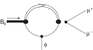
FIG. 1.: Direct diagram with $V,A,T$ currents changing $b\to s$. The momentum carried by the heavy quark is $m_{Q}v+\ell+k$ where $k$, the residual momentum $k\simeq\Lambda_{QCD}$, is due to the interaction of the heavy quark with the light degrees of freedom.

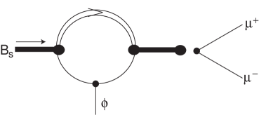
FIG. 2.: Polar diagram from $1^{-}$ and $1^{+}$ intermediate states.

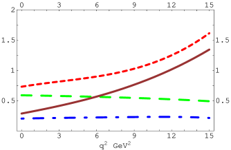
FIG. 3.: $q^{2}$ dependence of the semileptonic $B_{s}\to\phi$ form factors $V$ (dash-dotted), $A_{1}$ (large dashes), $A_{2}$ (small dashes) and $A_{0}$ (continuous line).

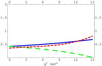
FIG. 4.: $q^{2}$ dependence of the tensor $B_{s}\to\phi$ form factors $T_{1}$ (continuous line), $T_{2}$ (large dashes) and $T_{3}$ (small dashes).

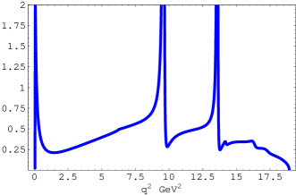
FIG. 5.: Dimuon invariant mass distribution of the $B_{s}\to\phi\mu^{+}\mu^{-}$ decay. The vertical axis is in units of $10^{-5}$ GeV^-2.

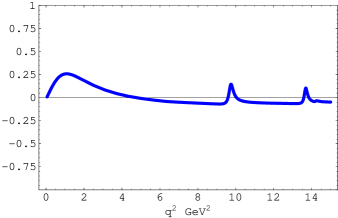
FIG. 6.: Normalized forward–backward asymmetry of the $B_{s}\to\phi\mu^{+}\mu^{-}$ decay. The two peaks at high $q^{2}$ values are due to the $J/\psi$ and $\psi(2S)$ resonances.