Abstract

R. P. Feynman was quite fond of inventing new physics. It is shown that some of his physical ideas can be supported by the mathematical instruments available from the Lorentz group. As a consequence, it is possible to construct a Lorentz-covariant picture of the parton model. It is shown first how the Lorentz group can be used for studying the internal space-time symmetries of relativistic particles. These symmetries are dictated by Wigner’s little groups, whose transformations leave the energy-momentum four-vector of a given particle invariant. The symmetry of massive particles is like the three-dimensional rotation group, while the symmetry of massless particles is locally isomorphic to the two-dimensional Euclidean group. It is noted that the $E(2)$-like symmetry of massless particles can be obtained as an infinite-momentum and/or zero-mass limit of the $O(3)$-like little group for massive particles. It is shown that the formalism can be extended to cover relativistic particles with space-time extensions, such as heavy ions and hadrons in the quark model. It is possible to construct representations of the little group using harmonic oscillators, which Feynman et al. used for studying relativistic extended hadrons. This oscillator formalism allows us to show that Feynman’s parton model is a Lorentz-boosted quark model. The formalism also allows us to explain in detail Feynman’s rest of the universe which is contained in his parton picture.

1 Introduction

The role of Lorentz covariance in quantum field theory and thus Feynman diagrams is well known. In this paper, we study how the Lorentz group plays roles in other physical theories initiated by Feynman. Richard Feynman and Eugene Wigner left their own legacies in physics. Their approaches to physics appear to be different. Feynman knew how to observe the real world and wrote down systematically how the physical world behaves, while Wigner was able to develop mathematical tools suitable to physics.

The most controversial phenomenological observation Feynman made was his parton model. Among the many contributions Wigner made, his 1939 paper on the inhomogeneous Lorentz group is still controversial in that its physical contents are still being explored. In this report, we propose to combine Feynman’s parton picture with Wigner’s representation of the Lorentz group. The paper thus consists of two parts. First, we explain in detail Wigner’s representation of the Lorentz group for internal space-time symmetries of relativistic particles. We then deal with Feynman’s world using coupled harmonic oscillators. It is shown that his parton model can be explained within the framework of Wigner’s representation.

In order to see which aspect of Wigner’s work is relevant to Feynmnan’s parton model, let us go back to Einstein. If the momentum of a particle is much smaller than its mass, the energy-momentum relation is $E=p^{2}/2m+mc^{2}$. If the momentum is much larger than the mass, the relation is $E=cp$. These two different relations can be combined into one covariant formula $E=\sqrt{m^{2}+p^{2}}$. This aspect of Einstein’s $E=mc^{2}$ is also well known.

In addition, particles have internal space-time variables. Massive particles have spins while massless particles have their helicities and gauge degrees of freedom. As a “further content” of Einstein’s $E=mc^{2}$, we shall discuss that the internal space-time structures of massive and massless particles can be unified into one covariant package, as $E=\sqrt{m^{2}+p^{2}}$ does for the energy-momentum relation.

The mathematical framework of this program was developed by Eugene Wigner in 1939 [1]. He constructed the maximal subgroups of the Lorentz group whose transformations will leave the four-momentum of a given particle invariant. These groups are known as Wigner’s little groups. Thus, the transformations of the little groups change the internal space-time variables of the particle, while leaving its four-momentum invariant. The little group is a covariant entity and takes different forms for particles moving with different speeds.

In order to achieve the zero-mass and/or infinite-momentum limit of the $O(3)$-like little group to obtain the $E(2)$-like little group, we use the group contraction technique introduced by Inonu and Wigner [2], who obtained the $E(2)$ group by taking a flat-surface approximation of a spherical surface at the north pole. In 1987, Kim and Wigner [3] observed that it is also possible to make a cylindrical approximation of the spherical surface around the equatorial belt. While the correspondence between $O(3)$ and the $O(3)$-like little group is transparent, the $E(2)$-like little group contains both the $E(2)$ group and the cylindrical group [4]. We study this aspect in detail in this report.

Let us look at the world of R. P. Feynman. When we read his papers, he totally avoids group theoretical languages. However, whenever appropriate, his physical reasoning is consistent with the Lorentz group. Let us look at Feynman diagrams. They are surprisingly consistent with Lorentz covariance of the S-matrix formalism of quantum field theory. This aspect is well known.

In this paper, we study Feynman’s papers published in 1969 [5] and 1971 [6], and the chapter on density matrix in his 1972 book on statistical mechanics [7]. Feynman appears to be dealing with three different physical problems in these three papers. However, the Lorentz group allows us to combine them into one great piece of work which includes a covariant description of Feynman’s parton picture.

How do we do this? In their 1971 paper [6], Feynman et al. used harmonic oscillators to work out hadronic mass spectra. Even though they used relativistic oscillators, they did not address the question of whether their formalism constitute a representation of Wigner’s little group. On the other hand, Wigner did not use harmonic oscillators too often in his papers, and Feynman did not pay enough attention to Lorentz covariance. Thus, in order to combine Feynman’s initiative with Wigner’s formalism, we can construct representations of the little group using harmonic oscillators. In so doing, we construct harmonic oscillator wave functions which can be Lorentz-boosted.

The question then is whether we can produce new physics by combining them. In this paper, we develop Wigner’s mathematical formalism first, and we then use it to interpret Feynman’s physics.

In Sec. 2, we present a brief history of applications of the little groups to internal space-time symmetries of relativistic particles. It is pointed out in Sec. 3 that the translation-like transformations of the $E(2)$-like little group corresponds to gauge transformations.

In Sec. 4, we discuss the contraction of the three-dimensional rotation group to the two-dimensional Euclidean group. In Sec. 5, we discuss the little group for a massless particle as the infinite-momentum and/or zero-mass limit of the little group for a massive particle.

In Sec. 6, we move into to the world of R. P. Feynman. Feynman was particularly fond of harmonic oscillators in formulating new ideas. It is pointed out that harmonic oscillators embrace many useful properties of the Lorentz group. In Sec. 7, we review the quantum mechanics of coupled harmonic oscillators in which one of them corresponds to the world in which we do physics, and the other is considered as the rest of the universe. In Sec. 8, it is shown that the time-separation variable in a two-body bound state belongs to Feynman’s rest of the universe. It is shown also that Feynman’s oscillator formalism includes this time-separation variable. We show in Sec. 9 that this $O(1,1)$ formalism enables to construct a covariant model of relativistic extended particles. As a consequence, we show that the quark and parton model are two different aspects of one covariant object. It is shown also that this parton picture exhibits the decoherence effect.

From the historical point of view, we are dealing here with further contents of Einstein’s energy-momentum relation. This question is addressed in Sec. 10.

2 Wigner’s Little Groups

The Poincaré group is the group of inhomogeneous Lorentz transformations, namely Lorentz transformations preceded or followed by space-time translations. In order to study this group, we have to understand first the group of Lorentz transformations, the group of translations, and how these two groups are combined to form the Poincaré group. The Poincaré group is a semi-direct product of the Lorentz and translation groups. The two Casimir operators of this group correspond to the (mass)² and (spin)² of a given particle. Indeed, the particle mass and its spin magnitude are Lorentz-invariant quantities.

The question then is how to construct the representations of the Lorentz group which are relevant to physics. For this purpose, Wigner in 1939 studied the subgroups of the Lorentz group whose transformations leave the four-momentum of a given free particle invariant [1]. The maximal subgroup of the Lorentz group which leaves the four-momentum invariant is called the little group. Since the little group leaves the four-momentum invariant, it governs the internal space-time symmetries of relativistic particles. Wigner shows in his paper that the internal space-time symmetries of massive and massless particles are dictated by the $O(3)$-like and $E(2)$-like little groups respectively.

The $O(3)$-like little group is locally isomorphic to the three-dimensional rotation group, which is very familiar to us. For instance, the group $SU(2)$ for the electron spin is an $O(3)$-like little group. The group $E(2)$ is the Euclidean group in a two-dimensional space, consisting of translations and rotations on a flat surface. We are performing these transformations everyday on ourselves when we move from home to school. The mathematics of these Euclidean transformations are also simple. However, the group of these transformations are not well known to us. In Sec. 4, we give a matrix representation of the $E(2)$ group.

The group of Lorentz transformations consists of three boosts and three rotations. The rotations therefore constitute a subgroup of the Lorentz group. If a massive particle is at rest, its four-momentum is invariant under rotations. Thus the little group for a massive particle at rest is the three-dimensional rotation group. Then what is affected by the rotation? The answer to this question is very simple. The particle in general has its spin. The spin orientation is going to be affected by the rotation!

If the rest-particle is boosted along the $z$ direction, it will pick up a non-zero momentum component. The generators of the $O(3)$ group will then be boosted. The boost will take the form of conjugation by the boost operator. This boost will not change the Lie algebra of the rotation group, and the boosted little group will still leave the boosted four-momentum invariant. We call this the $O(3)$-like little group.

We realize that the standard four-vector convention is $(t,x,y,z)$, but it is more convenient to use $(x,y,z,t)$ when we study light-cone coordinate system and group contractions. In this non-standard convention, the four-momentum vector for the particle at rest is $(0,0,0,m)$, and the three-dimensional rotation group leaves this four-momentum invariant. This little group is generated by

$$J_{1}=\pmatrix{0&0&0&0\cr 0&0&-i&0\cr 0&i&0&0\cr 0&0&0&0},\qquad J_{2}=\pmatrix{0&0&i&0\cr 0&0&0&0\cr-i&0&0&0\cr 0&0&0&0},\qquad J_{3}=\pmatrix{0&-i&0&0\cr i&0&0&0\cr 0&0&0&0\cr 0&0&0&0},$$ (1)

which satisfy the commutation relations:

$$[J_{i},J_{j}]=i\epsilon_{ijk}J_{k}.$$ (2)

It is not possible to bring a massless particle to its rest frame. In his 1939 paper [1], Wigner observed that the little group for a massless particle moving along the $z$ axis is generated by the rotation generator around the $z$ axis, namely $J_{3}$ of Eq.(1), and two other generators which take the form

$$N_{1}=\pmatrix{0&0&-i&i\cr 0&0&0&0\cr i&0&0&0\cr i&0&0&0},\qquad N_{2}=\pmatrix{0&0&0&0\cr 0&0&-i&i\cr 0&i&0&0\cr 0&i&0&0}.$$ (3)

If we use $K_{i}$ for the boost generator along the i-th axis, these matrices can be written as

$$N_{1}=K_{1}-J_{2},\qquad N_{2}=K_{2}+J_{1},$$ (4)

with

$$K_{1}=\pmatrix{0&0&0&i\cr 0&0&0&0\cr 0&0&0&0\cr i&0&0&0},\qquad K_{2}=\pmatrix{0&0&0&0\cr 0&0&0&i\cr 0&0&0&0\cr 0&i&0&0}.$$ (5)

The generators $J_{3},N_{1}$ and $N_{2}$ satisfy the following set of commutation relations.

$$[N_{1},N_{2}]=0,\qquad[J_{3},N_{1}]=iN_{2},\qquad[J_{3},N_{2}]=-iN_{1}.$$ (6)

In Sec. 4, we discuss the generators of the $E(2)$ group. They are $J_{3}$ which generates rotations around the $z$ axis, and $P_{1}$ and $P_{2}$ which generate translations along the $x$ and $y$ directions respectively. If we replace $N_{1}$ and $N_{2}$ by $P_{1}$ and $P_{2}$, the above set of commutation relations becomes the set given for the $E(2)$ group given in Eq.(18). This is the reason why we say the little group for massless particles is $E(2)$-like. Very clearly, the matrices $N_{1}$ and $N_{2}$ generate Lorentz transformations.

It is not difficult to associate the rotation generator $J_{3}$ with the helicity degree of freedom of the massless particle. Then what physical variable is associated with the $N_{1}$ and $N_{2}$ generators? Indeed, Wigner was the one who discovered the existence of these generators, but did not give any physical interpretation to these translation-like generators. For this reason, for many years, only those representations with the zero-eigenvalues of the $N$ operators were thought to be physically meaningful representations [8]. It was not until 1971 when Janner and Janssen reported that the transformations generated by these operators are gauge transformations [9, 10, 12]. The role of this translation-like transformation has also been studied for spin-1/2 particles, and it was concluded that the polarization of neutrinos is due to gauge invariance [11, 13].

Another important development along this line of research is the application of group contractions to the unifications of the two different little groups for massive and massless particles. We always associate the three-dimensional rotation group with a spherical surface. Let us consider a circular area of radius 1 kilometer centered on the north pole of the earth. Since the radius of the earth is more than 6,450 times longer, the circular region appears flat. Thus, within this region, we use the $E(2)$ symmetry group for this region. The validity of this approximation depends on the ratio of the two radii.

In 1953, Inonu and Wigner formulated this problem as the contraction of $O(3)$ to $E(2)$ [2]. How about then the little groups which are isomorphic to $O(3)$ and $E(2)$? It is reasonable to expect that the $E(2)$-like little group be obtained as a limiting case for of the $O(3)$-like little group for massless particles. In 1981, it was observed by Ferrara and Savoy that this limiting process is the Lorentz boost [14]. In 1983, using the same limiting process as that of Ferrara and Savoy, Han et al showed that transverse rotation generators become the generators of gauge transformations in the limit of infinite momentum and/or zero mass [15]. In 1987, Kim and Wigner showed that the little group for massless particles is the cylindrical group which is isomorphic to the $E(2)$ group [3]. This is illustrated in Fig. 1.

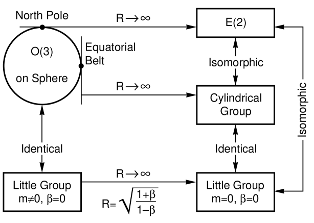
Figure 1: Contraction of O(3) to E(2) and to the cylindrical group, and contraction of the O(3)-like little group to the E(2)-like little group. The correspondence between E(2) and the E(2)-like little group is isomorphic but not identical. The cylindrical group is identical to the E(2)-like little group. The Lorentz boost of the O(3)-like little group for a massive particle is the same as the contraction of O(3) to the cylindrical group.

3 Translations and Gauge Transformations

It is possible to get the hint that the $N$ operators generate gauge transformations from Weinberg’s 1964 papers [8, 11]. But it was not until 1971 when Janner and Janssen explicitly demonstrated that they generate gauge transformations [9, 10]. In order to fully appreciate their work, let us compute the transformation matrix

$$\exp{(-i(uN_{1}+vN_{2})}$$ (7)

generated by $N_{1}$ and $N_{2}$. Then the four-by-four matrix takes the form

$$\pmatrix{1&0&-u&u\cr 0&1&-v&v\cr u&v&1-(u^{2}+v^{2})/2&(u^{2}+v^{2})/2\cr u&0&-(u^{2}+v^{2})/2&1+(u^{2}+v^{2})/2}.$$ (8)

If we apply this matrix to the four-vector to the four-momentum vector

$$p=(0,0,\omega,\omega)$$ (9)

of a massless particle, the momentum remains invariant. It therefore satisfies the condition for the little group. If we apply this matrix to the electromagnetic four-potential

$$A=(A_{1},A_{2},A_{3},A_{0})\exp{(i(kz-\omega t))},$$ (10)

with $A_{3}=A_{0}$ which is the Lorentz condition, the result is a gauge transformation. This is what Janner and Janssen discovered in their 1971 and 1972 papers [9]. Thus the matrices $N_{1}$ and $N_{2}$ generate gauge transformations.

4 Contraction of O(3) to E(2)

In this section, we explain what the $E(2)$ group is. We then explain how we can obtain this group from the three-dimensional rotation group by making a flat-surface or cylindrical approximation. This contraction procedure will give a clue to obtaining the $E(2)$-like symmetry for massless particles from the $O(3)$-like symmetry for massive particles by taking the infinite-momentum limit.

The $E(2)$ transformations consist of a rotation and two translations on a flat plane. Let us start with the rotation matrix applicable to the column vector $(x,y,1)$:

$$R(\theta)=\pmatrix{\cos\theta&-\sin\theta&0\cr\sin\theta&\cos\theta&0\cr 0&0&1}.$$ (11)

Let us then consider the translation matrix:

$$T(a,b)=\pmatrix{1&0&a\cr 0&1&b\cr 0&0&1}.$$ (12)

If we take the product $T(a,b)R(\theta)$,

$$E(a,b,\theta)=T(a,b)R(\theta)=\pmatrix{\cos\theta&-\sin\theta&a\cr\sin\theta&\cos\theta&b\cr 0&0&1}.$$ (13)

This is the Euclidean transformation matrix applicable to the two-dimensional $xy$ plane. The matrices $R(\theta)$ and $T(a,b)$ represent the rotation and translation subgroups respectively. The above expression is not a direct product because $R(\theta)$ does not commute with $T(a,b)$. The translations constitute an Abelian invariant subgroup because two different $T$ matrices commute with each other, and because

$$R(\theta)T(a,b)R^{-1}(\theta)=T(a^{\prime},b^{\prime}).$$ (14)

The rotation subgroup is not invariant because the conjugation

$$T(a,b)R(\theta)T^{-1}(a,b)$$ (15)

does not lead to another rotation.

We can write the above transformation matrix in terms of generators. The rotation is generated by

$$J_{3}=\pmatrix{0&-i&0\cr i&0&0\cr 0&0&0}.$$ (16)

The translations are generated by

$$P_{1}=\pmatrix{0&0&i\cr 0&0&0\cr 0&0&0},\qquad P_{2}=\pmatrix{0&0&0\cr 0&0&i\cr 0&0&0}.$$ (17)

These generators satisfy the commutation relations:

$$[P_{1},P_{2}]=0,\qquad[J_{3},P_{1}]=iP_{2},\qquad[J_{3},P_{2}]=-iP_{1}.$$ (18)

This $E(2)$ group is not only convenient for illustrating the groups containing an Abelian invariant subgroup, but also occupies an important place in constructing representations for the little group for massless particles, since the little group for massless particles is locally isomorphic to the above $E(2)$ group.

The contraction of $O(3)$ to $E(2)$ is well known and is often called the Inonu-Wigner contraction [2]. The question is whether the $E(2)$-like little group can be obtained from the $O(3)$-like little group. In order to answer this question, let us closely look at the original form of the Inonu-Wigner contraction. We start with the generators of $O(3)$. The $J_{3}$ matrix is given in Eq.(1), and

$$J_{2}=\pmatrix{0&0&i\cr 0&0&0\cr-i&0&0},\qquad J_{3}=\pmatrix{0&-i&0\cr i&0&0\cr 0&0&0}.$$ (19)

The Euclidean group $E(2)$ is generated by $J_{3},P_{1}$ and $P_{2}$, and their Lie algebra has been discussed in Sec. 1.

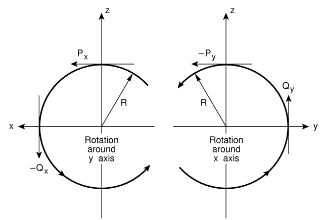
Figure 2: North-pole and Equatorial-belt approximations. The north-pole approximation leads to the contraction of O(3) to E(2). The equatorial-belt approximation leads corresponds to the contraction the cylindrical group.

Let us transpose the Lie algebra of the $E(2)$ group. Then $P_{1}$ and $P_{2}$ become $Q_{1}$ and $Q_{2}$ respectively, where

$$Q_{1}=\pmatrix{0&0&0\cr 0&0&0\cr i&0&0},\qquad Q_{2}=\pmatrix{0&0&0\cr 0&0&0\cr 0&i&0}.$$ (20)

Together with $J_{3}$, these generators satisfy the same set of commutation relations as that for $J_{3},P_{1}$, and $P_{2}$ given in Eq.(18):

$$[Q_{1},Q_{2}]=0,\qquad[J_{3},Q_{1}]=iQ_{2},\qquad[J_{3},Q_{2}]=-iQ_{1}.$$ (21)

These matrices generate transformations of a point on a circular cylinder. Rotations around the cylindrical axis are generated by $J_{3}$. The matrices $Q_{1}$ and $Q_{2}$ generate translations along the direction of $z$ axis. The group generated by these three matrices is called the cylindrical group [3, 4].

We can achieve the contractions to the Euclidean and cylindrical groups by taking the large-radius limits of

$$P_{1}={1\over R}B^{-1}J_{2}B,\qquad P_{2}=-{1\over R}B^{-1}J_{1}B,$$ (22)

and

$$Q_{1}=-{1\over R}BJ_{2}B^{-1},\qquad Q_{2}={1\over R}BJ_{1}B^{-1},$$ (23)

where

$$B(R)=\pmatrix{1&0&0\cr 0&1&0\cr 0&0&R}.$$ (24)

The vector spaces to which the above generators are applicable are $(x,y,z/R)$ and $(x,y,Rz)$ for the Euclidean and cylindrical groups respectively. They can be regarded as the north-pole and equatorial-belt approximations of the spherical surface respectively [3]. Fig. 2 illustrates how the Euclidean and cylindrical contractions are made.

5 Contraction of O(3)-like Little Group to E(2)-like Little Group

Since $P_{1}(P_{2})$ commutes with $Q_{2}(Q_{1})$, we can consider the following combination of generators.

$$F_{1}=P_{1}+Q_{1},\qquad F_{2}=P_{2}+Q_{2}.$$ (25)

Then these operators also satisfy the commutation relations:

$$[F_{1},F_{2}]=0,\qquad[J_{3},F_{1}]=iF_{2},\qquad[J_{3},F_{2}]=-iF_{1}.$$ (26)

However, we cannot make this addition using the three-by-three matrices for $P_{i}$ and $Q_{i}$ to construct three-by-three matrices for $F_{1}$ and $F_{2}$, because the vector spaces are different for the $P_{i}$ and $Q_{i}$ representations. We can accommodate this difference by creating two different $z$ coordinates, one with a contracted $z$ and the other with an expanded $z$, namely $(x,y,Rz,z/R)$. Then the generators become

$$P_{1}=\pmatrix{0&0&0&i\cr 0&0&0&0\cr 0&0&0&0\cr 0&0&0&0},\qquad P_{2}=\pmatrix{0&0&0&0\cr 0&0&0&i\cr 0&0&0&0\cr 0&0&0&0},$$ (27)

and

$$Q_{1}=\pmatrix{0&0&0&0\cr 0&0&0&0\cr i&0&0&0\cr 0&0&0&0},\qquad Q_{2}=\pmatrix{0&0&0&0\cr 0&0&0&0\cr 0&i&0&0\cr 0&0&0&0}.$$ (28)

Then $F_{1}$ and $F_{2}$ will take the form

$$F_{1}=\pmatrix{0&0&0&i\cr 0&0&0&0\cr i&0&0&0\cr 0&0&0&0},\qquad F_{2}=\pmatrix{0&0&0&0\cr 0&0&0&i\cr 0&i&0&0\cr 0&0&0&0}.$$ (29)

The rotation generator $J_{3}$ takes the form of Eq.(1). These four-by-four matrices satisfy the E(2)-like commutation relations of Eq.(26).

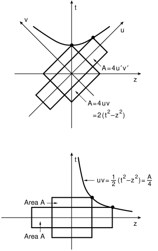
Figure 3: Light-cone coordinates. When the system is Lorentz-boosted, one of the axes expands while the other becomes contracted. Both the expansion and contraction are needed for the contraction of the $O(3)$-like little group to $E(2)$-like little group.

Now the $B$ matrix of Eq.(24), can be expanded to

$$B(R)=\pmatrix{1&0&0&0\cr 0&1&0&0\cr 0&0&R&0\cr 0&0&0&1/R}.$$ (30)

This matrix includes both the contraction and expansion in the light-cone coordinate system, as illustrated in Fig. 3. If we make a similarity transformation on the above form using the matrix

$$\pmatrix{1&0&0&0\cr 0&1&0&0\cr 0&0&1/\sqrt{2}&-1/\sqrt{2}\cr 0&0&1/\sqrt{2}&1/\sqrt{2}},$$ (31)

which performs a 45-degree rotation of the third and fourth coordinates, then this matrix becomes

$$\pmatrix{1&0&0&0\cr 0&1&0&0\cr 0&0&\cosh\eta&\sinh\eta\cr 0&0&\sinh\eta&\cosh\eta},$$ (32)

with $R=e^{\eta}$. This form is the Lorentz boost matrix along the $z$ direction. If we start with the set of expanded rotation generators $J_{3}$ of Eq.(1), and perform the same operation as the original Inonu-Wigner contraction given in Eq.(22), the result is

$$N_{1}={1\over R}B^{-1}J_{2}B,\qquad N_{2}=-{1\over R}B^{-1}J_{1}B,$$ (33)

where $N_{1}$ and $N_{2}$ are given in Eq.(3). The generators $N_{1}$ and $N_{2}$ are the contracted $J_{2}$ and $J_{1}$ respectively in the infinite-momentum and/or zero-mass limit.

It was noted in Sec. 3 that $N_{1}$ and $N_{2}$ generate gauge transformations on massless particles. Thus the contraction of the transverse rotations leads to gauge transformations.

We have seen in this section that Wigner’s $O(3)$-like little group can be contracted into the $E(2)$-like little group for massless particles. Here, we worked out explicitly for the spin-1 case, but this mechanism should be applicable to all other spins. Of particular interest is spin-1/2 particles. This has been studied by Han, Kim and Son [11]. They noted that there are also gauge transformations for spin-1/2 particles, and the polarization of neutrinos is a consequence of gauge invariance. It has also been shown that the gauge dependence of spin-1 particles can be traced to the gauge variable of the spin-1/2 particle [16]. It would be very interesting to see how the present formalism is applicable to higher-spin particles.

Another case of interest is the space-time symmetry of relativistic extended particles. In 1973 [17], the present authors constructed a ground-state harmonic oscillator wave function which can be Lorentz-boosted. It was later found that this oscillator formalism can be extended to represent the $O(3)$-like little group [18, 19]. This oscillator formalism has a stormy history because it ultimately plays a pivotal role in combining quantum mechanics and special relativity [20, 21].

With these wave functions, we propose to solve the following problem in high-energy physics. The quark model works well when hadrons are at rest or move slowly. However, when they move with speed close to that of light, they appear as a collection of an infinite-number of partons [5]. The question then is whether the parton model is a Lorentz-boosted quark model. This question has been addressed before [22, 23], but it can generate more interesting problems [24]. The present situation is presented in the Table 1.

Table 1: Massive and massless particles in one package. Wigner’s little group unifies the internal space-time symmetries for massive and massless particles. It is a great challenge for us to find another unification: the unification of the quark and parton pictures in high-energy physics.

	Massive, Slow	COVARIANCE	Massless, Fast
Energy-		Einstein’s
Momentum	$E=p^{2}/2m$	$E=[p^{2}+m^{2}]^{1/2}$	$E=p$
Internal	$S_{3}$		$S_{3}$
Space-time		Wigner’s
Symmetry	$S_{1},S_{2}$	Little Group	Gauge Trans.
Relativistic		One
Extended	Quark Model	Covariant	Parton Model
Particles		Theory

We are now ready to consider the third row of Table 1. In the this table, we would like to say that the quark model and the parton model are two different manifestation of one covariant entity. In order to appreciate fully this covariant aspect, let us examine Feynman’s style of doing physics.

6 Feynman’s World

Feynman was quite fond of using harmonic oscillators to probe new territories of physics. In this section, we examine which oscillator formalism is most suitable to interpret some of Feynman’s papers during the period 1969 – 1972. This formalism should accommodate special relativity and quantum mechanics of extended objects.

Let us start with a simple physical system. Two coupled harmonic oscillators play many important roles in physics. In group theory, it generates symmetry group as rich as $O(3,3)$ [25]. It has many interesting subgroups useful in all branches of physics. The group $O(3,1)$ is of course essential for studying covariance in special relativity. It is applicable to three space-like variables and one time-like variable. In the harmonic oscillator regime, those three space-like coordinates are separable. Thus, it is possible to separate longitudinal and transverse coordinates. If we leave out the transverse coordinates which do not participate in Lorentz boosts, the only relevant variables are longitudinal and time-like variables. The symmetry group for this case is $O(1,1)$ easily derivable from the Hamiltonian for the two-oscillator system.

It is widely known that this simple mathematical device is the basic language for two-photon coherent states known as squeezed states of light [26, 27]. However, this $O(1,1)$ device plays a much more powerful role in physics. According to Feynman, the adventure of our science of physics is a perpetual attempt to recognize that the different aspects of nature are really different aspects of the same thing [28]. Feynman wrote many papers on different subjects of physics, but they are coming from one paper according to him. We are not able to combine all of his papers, but we can consider three of his papers published during the period 1969-72.

In this paper, we would like to consider Feynman’s 1969 report on partons [5], the 1971 paper he published with his students on the quark model based on harmonic oscillators [6], and the chapter on density matrix in his 1972 book on statistical mechanics [7]. In these three different papers, Feynman deals with three distinct aspects of nature. We shall see whether Feynman was saying the same thing in these papers. For this purpose, we shall use the $O(1,1)$ symmetry derivable directly from the Hamiltonian for two coupled oscillators [29]. The standard procedure for this two-oscillator system is to separate the Hamiltonian using normal coordinates. The transformation to the normal coordinate system becomes very simple if the two oscillators are identical. We shall use this simple mathematics to find a common ground for the above-mentioned articles written by Feynman.

First, let us look at Feynman’s book on statistical mechanics [7]. He makes the following statement about the density matrix. When we solve a quantum-mechanical problem, what we really do is divide the universe into two parts - the system in which we are interested and the rest of the universe. We then usually act as if the system in which we are interested comprised the entire universe. To motivate the use of density matrices, let us see what happens when we include the part of the universe outside the system.

In order to see clearly what Feynman had in mind, we use the above-mentioned couples oscillators. One of the oscillators is the world in which we are interested and the other oscillator as the rest of the universe. There will be no effects on the first oscillator if the system is decoupled. Once coupled, we need a normal coordinate system in order separate the Hamiltonian. Then it is straightforward to write down the wave function of the system. Then the mathematics of this oscillator system is directly applicable to Lorentz-boosted harmonic oscillator wave functions, where one variable is the longitudinal coordinate and the other is the time variable. The system is uncoupled if the oscillator wave function is at rest, but the coupling becomes stronger as the oscillator is boosted to a high-speed Lorentz frame [19].

We shall then note that for two-body system, such as the hydrogen atom, there is a time-separation variable which is to be linearly mixed with the longitudinal space-separation variable. This space-separation variable is known as the Bohr radius, but we never talk about the time-separation variable in the present form of quantum mechanics, because this time-separation variable belongs to Feynman’s rest of the universe.

If we pretend not to know this time-separation variable, the entropy of the system will increase when the oscillator is boosted to a high-speed system [24]. Does this increase in entropy correspond to decoherence? Not necessarily. However, in 1969, Feynman observed the parton effect in which a rapidly moving hadron appears as a collection of incoherent partons [5]. This is the decoherence mechanism of current interest.

7 Two Coupled Oscillators

Two coupled harmonic oscillators serve many different purposes in physics. It is well known that this oscillator problem can be formulated into a problem of a quadratic equation in two variables. To make a long story short, let us consider a system of two identical oscillators coupled together by a spring. The Hamiltonian is

$$H={1\over 2m}\left\{p^{2}_{1}+p^{2}_{2}\right\}+{1\over 2}\left\{K\left(x_{1}^{2}+x^{2}_{2}\right)+2Cx_{1}x_{2}\right\}.$$ (34)

We are now ready to decouple this Hamiltonian by making the coordinate rotation:

$$y_{1}={1\over\sqrt{2}}\left(x_{1}-x_{2}\right),\qquad y_{2}={1\over\sqrt{2}}\left(x_{1}+x_{2}\right).$$ (35)

In terms of this new set of variables, the Hamiltonian can be written as

$$H={1\over 2m}\left\{p^{2}_{1}+p^{2}_{2}\right\}+{K\over 2}\left\{e^{2\eta}y^{2}_{1}+e^{-2\eta}y^{2}_{2}\right\},$$ (36)

with

$$\exp{(\eta)}=\sqrt{(K+C)/(K-C)}.$$ (37)

Thus $\eta$ measures the strength of the coupling. If $y_{1}$ and $y_{2}$ are measured in units of $(mK)^{1/4}$, the ground-state wave function of this oscillator system is

$$\psi_{\eta}(x_{1},x_{2})=\left({1\over{\pi}}\right)^{1/2}\exp{\left\{-{1\over 2}(e^{\eta}y^{2}_{1}+e^{-\eta}y^{2}_{2})\right\}}.$$ (38)

The wave function is separable in the $y_{1}$ and $y_{2}$ variables. However, for the variables $x_{1}$ and $x_{2}$, the story is quite different.

The key question is how quantum mechanical calculations in the world of the observed variable are affected when we average over the other variable. The $x_{2}$ space in this case corresponds to Feynman’s rest of the universe, if we only consider quantum mechanics in the $x_{1}$ space. As was discussed in the literature for several different purposes [27, 19], the wave function of Eq.(38) can be expanded as

$$\psi_{\eta}(x_{1},x_{2})={1\over\cosh\eta}\sum_{k}\left(\tanh{\eta\over 2}\right)^{k}\phi_{k}(x_{1})\phi_{k}(x_{2}).$$ (39)

This expansion corresponds to the two-photon coherent states in Yuen’s paper [26], and the wave function of Eq.(38) is a squeezed wave function [27].

The question then is what lessons we can learn from the situation in which we average over the $x_{2}$ variable. In order to study this problem, we use the density matrix. From this wave function, we can construct the pure-state density matrix

$$\rho(x_{1},x_{2};x_{1}^{\prime},x_{2}^{\prime})=\psi_{\eta}(x_{1},x_{2})\psi_{\eta}(x_{1}^{\prime},x_{2}^{\prime}),$$ (40)

If we are not able to make observations on the $x_{2}$, we should take the trace of the $\rho$ matrix with respect to the $x_{2}$ variable. Then the resulting density matrix is

$$\rho(x,x^{\prime})=\int\psi_{\eta}(x,x_{2})\left\{\psi_{\eta}(x^{\prime},x_{2})\right\}^{*}dx_{2}.$$ (41)

We have simplicity replaced $x_{1}$ and $x^{\prime}_{1}$ by $x$ and $x^{\prime}$ respectively. If we perform the integral of Eq.(41), the result is

$$\rho(x,x^{\prime})=\left({1\over\cosh(\eta/2)}\right)^{2}\sum_{k}\left(\tanh{\eta\over 2}\right)^{2k}\phi_{k}(x)\phi^{*}_{k}(x^{\prime}),$$ (42)

which leads to $Tr(\rho)=1$. It is also straightforward to compute the integral for $Tr(\rho^{2})$. The calculation leads to

$$Tr\left(\rho^{2}\right)=\left({1\over\cosh(\eta/2)}\right)^{4}\sum_{k}\left(\tanh{\eta\over 2}\right)^{4k}.$$ (43)

The sum of this series is $(1/\cosh\eta)$, which is smaller than one if the parameter $\eta$ does not vanish.

This is of course due to the fact that we are averaging over the $x_{2}$ variable which we do not measure. The standard way to measure this ignorance is to calculate the entropy defined as

$$S=-Tr\left(\rho\ln(\rho)\right),$$ (44)

where $S$ is measured in units of Boltzmann’s constant. If we use the density matrix given in Eq.(42), the entropy becomes

$$S=2\left\{\cosh^{2}\left({\eta\over 2}\right)\ln\left(\cosh{\eta\over 2}\right)-\sinh^{2}\left({\eta\over 2}\right)\ln\left(\sinh{\eta\over 2}\right)\right\}.$$ (45)

This expression can be translated into a more familiar form if we use the notation

$$\tanh{\eta\over 2}=\exp\left(-{\hbar\omega\over kT}\right),$$ (46)

where $\omega$ is given in Eq.(37) [30].

It is known in the literature that this rise in entropy and temperature causes the Wigner function to spread wide in phase space causing an increase of uncertainty [29]. Certainly, we cannot reach a classical limit by increasing the uncertainty. On the other hand, we are accustomed to think this entropy increase has something to do with decoherence, and we are also accustomed to think the lack of coherence has something to do with a classical limit. Are they compatible? We thus need a new vision in order to define precisely the word “decoherence.”

8 Time-separation Variable in Feynman’s Rest of the Universe

Quantum field theory has been quite successful in terms of perturbation techniques in quantum electrodynamics. However, this formalism is basically based on the S matrix for scattering problems and useful only for physically processes where a set of free particles becomes another set of free particles after interaction. Quantum field theory does not address the question of localized probability distributions and their covariance under Lorentz transformations. The Schrödinger quantum mechanics of the hydrogen atom deals with localized probability distribution. Indeed, the localization condition leads to the discrete energy spectrum. Here, the uncertainty relation is stated in terms of the spatial separation between the proton and the electron. If we believe in Lorentz covariance, there must also be a time separation between the two constituent particles.

Before 1964 [31], the hydrogen atom was used for illustrating bound states. These days, we use hadrons which are bound states of quarks. Let us use the simplest hadron consisting of two quarks bound together with an attractive force, and consider their space-time positions $x_{a}$ and $x_{b}$, and use the variables

$$X=(x_{a}+x_{b})/2,\qquad x=(x_{a}-x_{b})/2\sqrt{2}.$$ (47)

The four-vector $X$ specifies where the hadron is located in space and time, while the variable $x$ measures the space-time separation between the quarks. According to Einstein, this space-time separation contains a time-like component which actively participates as can be seen from

$$\pmatrix{z^{\prime}\cr t^{\prime}}=\pmatrix{\cosh\eta&\sinh\eta\cr\sinh\eta&\cosh\eta}\pmatrix{z\cr t},$$ (48)

when the hadron is boosted along the $z$ direction. In terms of the light-cone variables defined as [32]

$$u=(z+t)/\sqrt{2},\qquad v=(z-t)/\sqrt{2}.$$ (49)

The boost transformation of Eq.(48) takes the form

$$u^{\prime}=e^{\eta}u,\qquad v^{\prime}=e^{-\eta}v.$$ (50)

The $u$ variable becomes expanded while the $v$ variable becomes contracted.

Does this time-separation variable exist when the hadron is at rest? Yes, according to Einstein. In the present form of quantum mechanics, we pretend not to know anything about this variable. Indeed, this variable belongs to Feynman’s rest of the universe. In this report, we shall see the role of this time-separation variable in decoherence mechanism.

Also in the present form of quantum mechanics, there is an uncertainty relation between the time and energy variables. However, there are no known time-like excitations. Unlike Heisenberg’s uncertainty relation applicable to position and momentum, the time and energy separation variables are c-numbers, and we are not allowed to write down the commutation relation between them. Indeed, the time-energy uncertainty relation is a c-number uncertainty relation [33], as is illustrated in Fig. 4

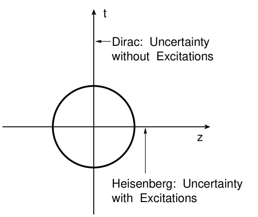
Figure 4: Space-time picture of quantum mechanics. There are quantum excitations along the space-like longitudinal direction, but there are no excitations along the time-like direction. The time-energy relation is a c-number uncertainty relation.

How does this space-time asymmetry fit into the world of covariance [17]. This question was studied in depth by the present authors. The answer is that Wigner’s $O(3)$-like little group is not a Lorentz-invariant symmetry, but is a covariant symmetry [1]. It has been shown that the time-energy uncertainty applicable to the time-separation variable fits perfectly into the $O(3)$-like symmetry of massive relativistic particles [19].

The c-number time-energy uncertainty relation allows us to write down a time distribution function without excitations [19]. If we use Gaussian forms for both space and time distributions, we can start with the expression

$$\left({1\over\pi}\right)^{1/2}\exp{\left\{-{1\over 2}\left(z^{2}+t^{2}\right)\right\}}$$ (51)

for the ground-state wave function. What do Feynman et al. say about this oscillator wave function?

In his classic 1971 paper [6], Feynman et al. start with the following Lorentz-invariant differential equation.

$${1\over 2}\left\{x^{2}_{\mu}-{\partial^{2}\over\partial x_{\mu}^{2}}\right\}\psi(x)=\lambda\psi(x).$$ (52)

This partial differential equation has many different solutions depending on the choice of separable variables and boundary conditions. Feynman et al. insist on Lorentz-invariant solutions which are not normalizable. On the other hand, if we insist on normalization, the ground-state wave function takes the form of Eq.(51). It is then possible to construct a representation of the Poincaré group from the solutions of the above differential equation [19]. If the system is boosted, the wave function becomes

$$\psi_{\eta}(z,t)=\left({1\over\pi}\right)^{1/2}\exp\left\{-{1\over 2}\left(e^{-2\eta}u^{2}+e^{2\eta}v^{2}\right)\right\}.$$ (53)

This wave function becomes Eq.(51) if $\eta$ becomes zero. The transition from Eq.(51) to Eq.(53) is a squeeze transformation. The wave function of Eq.(51) is distributed within a circular region in the $uv$ plane, and thus in the $zt$ plane. On the other hand, the wave function of Eq.(53) is distributed in an elliptic region with the light-cone axes as the major and minor axes respectively. If $\eta$ becomes very large, the wave function becomes concentrated along one of the light-cone axes. Indeed, the form given in Eq.(53) is a Lorentz-squeezed wave function. This squeeze mechanism is illustrated in Fig. 5.

It is interesting to note that the Lorentz-invariant differential equation of Eq.(52) contains the time-separation variable which belongs to Feynman’s rest of the universe. Furthermore, the wave function of Eq.(51) is identical to that of Eq.(38) for the coupled oscillator system, if the variables $z$ and $t$ are replaced $x_{1}$ and $x_{2}$ respectively. Thus the entropy increase due to the unobservable $x_{2}$ variable is applicable to the unobserved time-separation variable $t$.

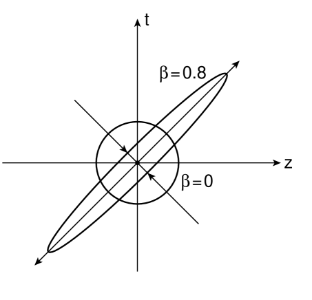
Figure 5: Effect of the Lorentz boost on the space-time wave function. The circular space-time distribution at the rest frame becomes Lorentz-squeezed to become an elliptic distribution.

9 Feynman’s Parton Picture

It is a widely accepted view that hadrons are quantum bound states of quarks having localized probability distribution. As in all bound-state cases, this localization condition is responsible for the existence of discrete mass spectra. The most convincing evidence for this bound-state picture is the hadronic mass spectra which are observed in high-energy laboratories [6, 19]. However, this picture of bound states is applicable only to observers in the Lorentz frame in which the hadron is at rest. How would the hadrons appear to observers in other Lorentz frames? To answer this question, can we use the picture of Lorentz-squeezed hadrons discussed in Sec. 8.

The radius of the proton is $10^{-5}$ of that of the hydrogen atom. Therefore, it is not unnatural to assume that the proton has a point charge in atomic physics. However, while carrying out experiments on electron scattering from proton targets, Hofstadter in 1955 observed that the proton charge is spread out [34]. In this experiment, an electron emits a virtual photon, which then interacts with the proton. If the proton consists of quarks distributed within a finite space-time region, the virtual photon will interact with quarks which carry fractional charges. The scattering amplitude will depend on the way in which quarks are distributed within the proton. The portion of the scattering amplitude which describes the interaction between the virtual photon and the proton is called the form factor.

Although there have been many attempts to explain this phenomenon within the framework of quantum field theory, it is quite natural to expect that the wave function in the quark model will describe the charge distribution. In high-energy experiments, we are dealing with the situation in which the momentum transfer in the scattering process is large. Indeed, the Lorentz-squeezed wave functions lead to the correct behavior of the hadronic form factor for large values of the momentum transfer [35].

Furthermore, in 1969, Feynman observed that a fast-moving hadron can be regarded as a collection of many “partons” whose properties do not appear to be quite different from those of the quarks [5]. For example, the number of quarks inside a static proton is three, while the number of partons in a rapidly moving proton appears to be infinite. The question then is how the proton looking like a bound state of quarks to one observer can appear different to an observer in a different Lorentz frame? Feynman made the following systematic observations.

• The picture is valid only for hadrons moving with velocity close to that of light.

• The interaction time between the quarks becomes dilated, and partons behave as free independent particles.

• The momentum distribution of partons becomes widespread as the hadron moves fast.

• The number of partons seems to be infinite or much larger than that of quarks.

Because the hadron is believed to be a bound state of two or three quarks, each of the above phenomena appears as a paradox, particularly b) and c) together.

In order to resolve this paradox, let us write down the momentum-energy wave function corresponding to Eq.(53). If the quarks have the four-momenta $p_{a}$ and $p_{b}$, we can construct two independent four-momentum variables [6]

$$P=p_{a}+p_{b},\qquad q=\sqrt{2}(p_{a}-p_{b}),$$ (54)

where $P$ is the total four-momentum and is thus the hadronic four-momentum. $q$ measures the four-momentum separation between the quarks. Their light-cone variables are

$$q_{u}=(q_{0}-q_{z})/\sqrt{2},\qquad q_{v}=(q_{0}+q_{z})/\sqrt{2}.$$ (55)

The resulting momentum-energy wave function is

$$\phi_{\eta}(q_{z},q_{0})=\left({1\over\pi}\right)^{1/2}\exp\left\{-{1\over 2}\left(e^{-2\eta}q_{u}^{2}+e^{2\eta}q_{v}^{2}\right)\right\}.$$ (56)

Because we are using here the harmonic oscillator, the mathematical form of the above momentum-energy wave function is identical to that of the space-time wave function. The Lorentz squeeze properties of these wave functions are also the same. This aspect of the squeeze has been exhaustively discussed in the literature [19, 22, 23].

When the hadron is at rest with $\eta=0$, both wave functions behave like those for the static bound state of quarks. As $\eta$ increases, the wave functions become continuously squeezed until they become concentrated along their respective positive light-cone axes. Let us look at the z-axis projection of the space-time wave function. Indeed, the width of the quark distribution increases as the hadronic speed approaches that of the speed of light. The position of each quark appears widespread to the observer in the laboratory frame, and the quarks appear like free particles.

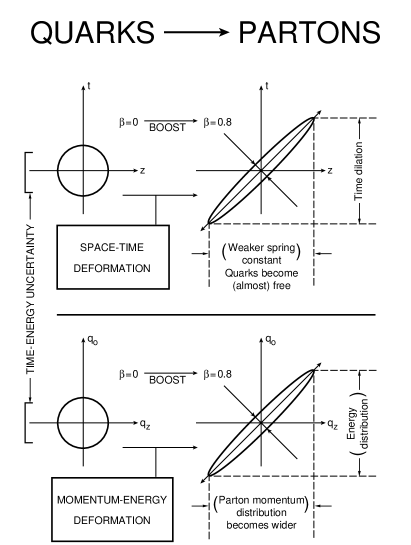
Figure 6: Lorentz-squeezed space-time and momentum-energy wave functions. As the hadron’s speed approaches that of light, both wave functions become concentrated along their respective positive light-cone axes. These light-cone concentrations lead to Feynman’s parton picture.

The momentum-energy wave function is just like the space-time wave function, as is shown in Fig. 6. The longitudinal momentum distribution becomes wide-spread as the hadronic speed approaches the velocity of light. This is in contradiction with our expectation from nonrelativistic quantum mechanics that the width of the momentum distribution is inversely proportional to that of the position wave function. Our expectation is that if the quarks are free, they must have their sharply defined momenta, not a wide-spread distribution.

However, according to our Lorentz-squeezed space-time and momentum-energy wave functions, the space-time width and the momentum-energy width increase in the same direction as the hadron is boosted. This is of course an effect of Lorentz covariance. This indeed is the key to the resolution of the quark-parton paradox [19, 22].

The most puzzling problem in the parton picture is that partons in the hadron appear as incoherent particles, while quarks are coherent when the hadron is at rest. Does this mean that the coherence is destroyed by the Lorentz boost? The answer is NO, and here is the resolution to this puzzle.

When the hadron is boosted, the hadronic matter becomes squeezed and becomes concentrated in the elliptic region along the positive light-cone axis, as is illustrated in Figs. 5 and 6. The length of the major axis becomes expanded by $e^{\eta}$, and the minor axis is contracted by $e^{\eta}$.

This means that the interaction time of the quarks among themselves become dilated. Because the wave function becomes wide-spread, the distance between one end of the harmonic oscillator well and the other end increases. This effect, first noted by Feynman [5], is universally observed in high-energy hadronic experiments. The period is oscillation increases like $e^{\eta}$.

On the other hand, the interaction time with the external signal, since it is moving in the direction opposite to the direction of the hadron, travels along the negative light-cone axis. If the hadron contracts along the negative light-cone axis, the interaction time decreases by $e^{-\eta}$. The ratio of the interaction time to the oscillator period becomes $e^{-2\eta}$. The energy of each proton coming out of the Fermilab accelerator is $900GeV$. This leads the ratio to $10^{-6}$. This is indeed a small number. The external signal is not able to sense the interaction of the quarks among themselves inside the hadron.

Indeed, Feynman’s parton picture is one concrete physical example where the decoherence effect is observed. As for the entropy, the time-separation variable belongs to the rest of the universe. Because we are not able to observe this variable, the entropy increases as the hadron is boosted to exhibit the parton effect. The decoherence is thus accompanied by an entropy increase.

Let us go back to the coupled-oscillator system. The light-cone variables in Eq.(53) correspond to the normal coordinates in the coupled-oscillator system given in Eq.(35). According to Feynman’s parton picture, the decoherence mechanism is determined by the ratio of widths of the wave function along the two normal coordinates. The result is listed in the third row of Table 1.

10 Further Contents of Einstein’s Formula for Energy, Mass, and Momentum

In Table 1, we put Wigner’s formalism and Feynman’s observation into a single package which could be called “Further Contents of Einstein’s $E=mc^{2}$.” To physicists, $E=mc^{2}$ means $E=\sqrt{m^{2}+p^{2}}$. Of course, the mass $m$ has different meanings for these two different formulas, one for the rest mass and the other for moving mass. This distinction is so obvious to physicists that there is a tendency not to mention it in the physics literature.

However, the distinction is not so trivial to those who study how special relativity was developed. Indeed, there has been a recent debate on this issue, and the debate is likely to continue. However, the present authors have not done enough research on this issue, but would like to acknowledge a very comprehensive review article by Okun [36], entitled “Concept of Mass” and comments on this article by various authors.

It is not clear whether Einstein was concerned with the question of whether the particles are point particles or objects with internal space-time structures, because the internal space-time symmetry was not formulated until 1939 when Wigner published his paper based on the little groups [1]. On the otherhand, Wigner’s approach starts from Einstein’s energy-momentum relation for free particles. Thus, the energy-momentum relation remains valid for particles with internal structure only if there is a covariant description of internal space-time symmetries. Indeed, this is the main point of the present paper.

Table 2: Historical Necessity. Newtonian Mechanics is Galilean-covariant, and Maxwell’s theory is Lorentz-covariant. Do they have to be based on two different kind of covariance?

	Galilean Covariance	Lorentz Covariance
Newtonian Mechanics	YES	NO
Maxwell Theory	NO	YES

Another historical question is who formulated the mathematics for special relativity. Here, prominent names are Lorentz, Poincaré and Minkowski. This is also an interesting and important issue. The present authors have done some research along this line, but not enough to make an impact on the existing literature.

The following point is well known, but seldom mentioned. Before Einstein, Newtonian mechanics and Maxwell’s equations were based on two different covariance principles, as is summarized in Table 2. Thus the development of special relativity is of historical necessity to those, like Einstein, who believed this world is one covariant world.

It is now firmly established that mechanics should also be Lorentz-covariant. Furthermore, it is a well-accepted view that Lorentz covariance should become Galilean covariance for slow particles. This slow-speed limit is not as trivial as taking a numerical limit of speed of particle divided by the speed of light. This limiting process was worked out by Inonu and Wigner in their 1953 paper [2], where they introduced group contractions. The Inonu-Wigner group contraction also allows us to take a large-speed limit, which we used in the present paper. It is interesting to note that both limiting processes can be derived from the Inonu-Wigner contraction.

References

- [1] E. P. Wigner, Ann. Math. 40, 149 (1939).
- [2] E. Inonu and E. P. Wigner, Proc. Natl. Acad. Scie. (U.S.A.) 39, 510 (1953).
- [3] Y. S. Kim and E. P. Wigner, J. Math. Phys. 28, 1175 (1987).
- [4] Y. S. Kim and E. P. Wigner, J. Math. Phys. 31, 55 (1990).
- [5] R. P. Feynman, The Behavior of Hadron Collisions at Extreme Energies, in High Energy Collisions, Proceedings of the Third International Conference, Stony Brook, New York, edited by C. N. Yang et al., Pages 237-249 (Gordon and Breach, New York, 1969).
- [6] R. P. Feynman, M. Kislinger, and F. Ravndal, Phys. Rev. D 3, 2706 (1971).
- [7] R. P. Feynman, Statistical Mechanics (Benjamin/Cummings, Reading, MA, 1972).
- [8] S. Weinberg, Phys. Rev. 134, B882 (1964); ibid. 135, B1049 (1964).
- [9] A. Janner and T. Janssen, Physica 53, 1 (1971); ibid. 60, 292 (1972).
- [10] For later papers on this problem, see J. Kuperzstych, Nuovo Cimento 31B, 1 (1976); D. Han and Y. S. Kim, Am. J. Phys. 49, 348 (1981); J. J. van der Bij, H. van Dam, and Y. J. Ng, Physica 116A, 307 (1982).
- [11] D. Han, Y. S. Kim, and D. Son, Phys. Rev. D 26, 3717 (1982).
- [12] Y. S. Kim, in Symmetry and Structural Properties of Condensed Matter, Proceedings 4th International School of Theoretical Physics (Zajaczkowo, Poland), edited by T. Lulek, W. Florek, and B. Lulek (World Scientific, 1997).
- [13] Y. S. Kim, in Quantum Systems: New Trends and Methods, Proceedings of the International Workshop (Minsk, Belarus), edited by Y. S. Kim, L. M. Tomil’chik, I. D. Feranchuk, and A. Z. Gazizov (World Scientific, 1997).
- [14] S. Ferrara and C. Savoy, in Supergravity 1981, S. Ferrara and J. G. Taylor eds. (Cambridge Univ. Press, Cambridge, 1982), p. 151. See also P. Kwon and M. Villasante, J. Math. Phys. 29, 560 (1988); ibid. 30, 201 (1989). For earlier papers on this subject, see H. Bacry and N. P. Chang, Ann. Phys. 47, 407 (1968); S. P. Misra and J. Maharana, Phys. Rev. D 14, 133 (1976).
- [15] D. Han, Y. S. Kim, and D. Son, Phys. Lett. B 131, 327 (1983). See also D. Han, Y. S. Kim, M. E. Noz, and D. Son, Am. J. Phys. 52, 1037 (1984).
- [16] D. Han, Y. S. Kim, and D. Son, J. Math. Phys. 27, 2228 (1986).
- [17] Y. S. Kim and M. E. Noz, Phys. Rev. D 8, 3521 (1973).
- [18] Y. S. Kim, M. E. Noz and S. H. Oh, J. Math. Phys. 20, 1341 (1979).
- [19] Y. S. Kim and M. E. Noz, Theory and Applications of the Poincaré Group (Reidel, Dordrecht, 1986).
- [20] P. A. M. Dirac, Proc. Roy. Soc. (London) A183, 284 (1945).
- [21] H. Yukawa, Phys. Rev. 91, 415 (1953).
- [22] Y. S. Kim and M. E. Noz, Phys. Rev. D 15, 335 (1977).
- [23] Y. S. Kim, Phys. Rev. Lett. 63, 348 (1989).
- [24] Y. S. Kim and E. P. Wigner, Phys. Lett. A 147, 343 (1990).
- [25] D. Han, Y. S. Kim, and M. E. Noz, J. Math. Phys. 36, 3940 (1995).
- [26] H. P. Yuen, Phys. Rev. A 13, 2226 (1976).
- [27] Y. S. Kim and M. E. Noz, Phase Space Picture of Quantum Mechanics (World Scientific, Singapore, 1991).
- [28] R. P. Feynman, http://www.aip.org/history/esva/exhibits/feynman.htm, (the Feynman page of the Emilio Segre Visual Archives of the American Institute of Physics)
- [29] D. Han, Y. S. Kim, and M. E. Noz, Am. J. Phys. 67, 61 (1999).
- [30] D. Han, Y. S. Kim, and Marilyn E. Noz, Phys. Lett. A 144, 111 (1989).
- [31] M. Gell-Mann, Phys. Lett. 13, 598 (1964).
- [32] P. A. M. Dirac, Rev. Mod. Phys. 21, 392 (1949).
- [33] P. A. M. Dirac, Proc. Roy. Soc. (London) A114, 234 and 710 (1927).
- [34] R. Hofstadter and R. W. McAllister, Phys. Rev. 98, 217 (1955).
- [35] K. Fujimura, T. Kobayashi, and M. Namiki, Prog. Theor. Phys. 43, 73 (1970).
- [36] L. B. Okun, Physics Today, June 1989, pp. 31 - 36. See also the letters from W. Rindler, M. Vnayck, P. Muragesan, S. Ruschin, C. Sauter, and L. B. Okun, Physics Today, May 1990, pp.13, 115 - 117.