TTP01-12

Determination of the bottom quark mass from the $\Upsilon(1S)$ system
Antonio Pineda
Institut für Theoretische Teilchenphysik
Universität Karlsruhe, D-76128 Karlsruhe, Germany

We approximately compute the normalization constant of the first infrared renormalon of the pole mass (and the singlet static potential). Estimates of higher order terms in the perturbative relation between the pole mass and the $\overline{\rm MS}$ mass (and in the relation between the singlet static potential and $\alpha_{s}$) are given. We define a matching scheme (the renormalon subtracted scheme) between QCD and any effective field theory with heavy quarks where, besides the usual perturbative matching, the first renormalon in the Borel plane of the pole mass is subtracted. A determination of the bottom $\overline{\rm MS}$ quark mass from the $\Upsilon(1S)$ system is performed with this new scheme and the errors studied. Our result reads $m_{b,\overline{\rm MS}}(m_{b,\overline{\rm MS}})=4\,210^{+90}_{-90}({\rm theory})^{-25}_{+25}(\alpha_{s})$ MeV. Using the mass difference between the $B$ and $D$ meson, we also obtain a value for the charm quark mass: $m_{c,\overline{\rm MS}}(m_{c,\overline{\rm MS}})=1\,210^{+70}_{-70}({\rm theory})^{+65}_{-65}(m_{b,\overline{\rm MS}})^{-45}_{+45}(\lambda_{1})$ MeV. We finally discuss upon eventual improvements of these determinations.
PACS numbers: 14.65.Fy, 14.65.Dw, 12.38.Cy, 12.39.Hg

1 Introduction

Systems composed by heavy quarks are very important in the study of the QCD dynamics. This is due to the fact that they can test QCD in a kinematical regime otherwise unreachable with only light quarks. They are characterized by having an scale, the mass of the heavy quark, much larger than any other dynamical scale in the problem. Therefore, it seems reasonable to study these systems by using effective field theories where the mass has been used as an expansion parameter. Some examples of such are HQET [1] for the the one-heavy quark sector and NRQCD [2] or pNRQCD [3, 4] for the $Q$-$\bar{Q}$ sector.

On general grounds, the matching coefficients of the (QCD) effective theories suffer from renormalon ambiguities [5] (for a review on renormalons see [6]). This means that, in principle, one can not compute these matching coefficients with infinity accuracy in terms of the (short distance physics) parameters of the underlying theory. From a formal point of view, there is not fundamental problem related with these ambiguities, since the renormalon ambiguities of the matching coefficients cancel with the renormalon ambiguities in the calculation of the matrix elements in the effective theory in such a way that observables are renormalon free (as they should be) up to the order in the expansion parameters to which the calculation has been performed.

Being more specific, a generic matching coefficient $c(\nu/m)$ would have the following perturbative expansion in $\alpha_{s}$:

$$c(\nu/m)=\bar{c}+\sum_{n=0}^{\infty}c_{n}\alpha_{s}^{n+1},$$ (1)

where $\alpha_{s}$ (in the $\overline{\rm MS}$ scheme) is normalized at the scale $\nu$. Its Borel transform would be

$$B[c](t)\equiv\sum_{n=0}^{\infty}c_{n}{t^{n}\over n!},$$ (2)

and $c$ is written in terms of its Borel transform as

$$c=\bar{c}+\int\limits_{0}^{\infty}\mbox{d}t\,e^{-t/\alpha_{s}}\,B[c](t).$$ (3)

The ambiguity in the matching coefficient reflects in poles in the Borel transform. If we take the one closest to the origin,

$$\delta B[c](t)\sim{1\over a-t},$$ (4)

where $a$ is a positive number, it sets up the maximal accuracy with which one can obtain the matching coefficients from a perturbative calculation, which is (roughly) of the order of

$$\delta c\sim r_{n^{*}}\alpha_{s}^{n^{*}},$$ (5)

where $n^{*}\sim{a\over\alpha_{s}}$. Moreover, the fact that $a$ is positive means that, even after Borel resummation, $c$ suffers from a non-perturbative ambiguity of order

$$\delta c\sim\left(\Lambda_{\rm QCD}\right)^{a\beta_{0}\over 2\pi}\,.$$ (6)

Figure 1: Symbolic relation between observables through the determination of the matching coefficients of the effective field theory.

As we have mentioned, these renormalon ambiguities will cancel anyhow in the final calculation of the observable. Therefore, we could ask ourselves why bother about this problem. The answer comes from the procedure we use to relate (and then predict) observables (see Fig. 1). Schematically, one takes one observable to fix the matching coefficient. In order to relate the matching coefficient with the observable, we use the effective field theory as a tool to provide the power counting rules in the calculation. Since we are relating one observable (a renormalon free object) with a matching coefficient suffering of some renormalon ambiguity, there must be another source of renormalon ambiguity as to cancel this one. As we have mentioned, the latter comes from the calculation of the matrix element in the effective theory. There is a problem here, however. If the matrix element in the effective theory is a non-perturbative object, the ambiguity of the matching coefficient is of the same size than this non-perturbative object that we do not know how to calculate anyhow. Nevertheless, if the matrix element in the effective theory is a perturbative object, the only way it has to show the renormalon is in a bad perturbative behavior in the expansion parameters in the effective theory (what is happening is that the coefficients that multiply the expansion parameters are not of $O(1)$ due to the renormalon, i.e. the renormalon is breaking down the assumption of naturalness implicit in any effective theory). This may seem irrelevant since the ambiguity is the same in either case but in the latter situation it means that the observable is less sensitive to long distance than the matching coefficient itself. Thus, if, for instance, we wanted later on to get the short distance parameters from that (weakly sensitive to long distance physics) observable, we are not doing an optimal job, since we use an intermediate parameter (the matching coefficient) that can not be obtained with better accuracy than the ones displayed in Eqs. (5)-(6), whereas the observable (and the short distance parameter) is less sensitive to long distance physics (the same problem will also appear if we want to relate two weakly sensitive to long distance physics observables through a more long distance sensitive matching coefficient). We can consider three examples (observables) to illustrate this point: the mass of the meson $B$ ($M_{B}$), the inclusive semileptonic decay width of the $B$ ($\Gamma(B\rightarrow X_{u}l\nu)$) and the mass of $\Upsilon(1S)$ (assuming in this latter case $m\alpha_{s}^{2}\gg\Lambda_{\rm QCD}$ for illustration). For these observables, the first non-perturbative corrections (leaving aside renormalons) are of the following type:

$$\delta_{np}M_{B}\sim\Lambda_{\rm QCD},\qquad\delta_{np}\Gamma(B\rightarrow X_{u}l\nu)\sim G_{F}^{2}m_{\rm OS}^{3}\Lambda_{\rm QCD}^{2},\qquad\delta_{np}M_{\Upsilon(1S)}\sim m_{\rm OS}{\Lambda_{\rm QCD}^{4}\over(m_{\rm OS}\alpha_{s})^{4}}\,,$$ (7)

where $m_{\rm OS}$ is the pole mass. The above results only become true if the perturbative piece can be computed with such precision. Nevertheless, this is not true in the on-shell (OS) scheme, where one uses the pole mass as an expansion parameter, since the latter suffers from renormalon ambiguities [7, 8]. Therefore, effectively, the above observables can only be computed perturbatively (working with the pole mass) with the following precision

$$\delta_{np}^{({\rm pert.})}M_{B}\sim\Lambda_{\rm QCD},\qquad\delta_{np}^{({\rm pert.})}\Gamma(B\rightarrow X_{u}l\nu)\sim G_{F}^{2}m_{\rm OS}^{4}\Lambda_{\rm QCD},\qquad\delta_{np}^{({\rm pert.})}M_{\Upsilon(1S)}\sim\Lambda_{\rm QCD}.$$ (8)

For the first observable this discussion is irrelevant but not for the other two, which become rather less well known that they could be.

Roughly speaking, the above discussion means that the renormalon of the matching coefficients can be spurious (it is not related to a real non-perturbative contribution in the observable) or real (it is related to a real non-perturbative contribution in the observable). In fact, this distinction depends on the observable we are considering rather than on the renormalon of the matching coefficient itself. The point we want to stress is that at the matching calculation level it makes no sense this distinction. Therefore, there is no necessity to keep the renormalon ambiguity (that it only appears due to the specific factorization prescription we are using) in the matching coefficients (even more if we take into account that its only role is to worsen the perturbative expansion in the matching coefficients). Thus, our proposal is that one should figure out a matching scheme where the renormalon ambiguity is subtracted from the matching coefficients. This is the program we will pursue here for the specific case of effective field theories with heavy quarks. In principle, the same program should, eventually, be carried out with other effective theories. Nevertheless, the worsening of the perturbative expansion was especially evident in effective theories with heavy quarks. This is due to the fact that the renormalon singularities lie close together to the origin and that perturbative calculations have gone very far in this case [9]-[22]. In other effective field theories this problem may have not become so acute (yet) but it may become relevant in the future.

The structure of the paper is as follows. In the next section, we compute the normalization constant of the first infrared (IR) renormalon of the pole mass. We also give estimates of the higher order coefficients of the perturbative series relating the pole mass with the $\overline{\rm MS}$ mass. In section 3, we compute the normalization constant of the first IR renormalon of the singlet static potential and also estimates of the higher order perturbative terms in the potential are given. In section 4, new definitions of the pole mass and the singlet static potential are given, within an effective field theory perspective, by subtracting their closest singularities to the origen in the Borel plane. In section 5, we provide a determination of the bottom $\overline{\rm MS}$ mass from the $\Upsilon(1S)$ mass and an estimate of the errors within this new approach. In section 6, we provide a determination of the charm $\overline{\rm MS}$ mass by using the mass difference between the $B$ and $D$ mesons. In section 7, we give our conclusions and discuss how to improve our determinations of the bottom and charm masses.

2 Mass normalization constant

The pole mass can be related to the $\overline{\rm MS}$ renormalized mass – which in principle can be measured to any accuracy at a very high energy scale – by the series

$$m_{\rm OS}=m_{\overline{\rm MS}}+\sum_{n=0}^{\infty}r_{n}\alpha_{s}^{n+1}\,,$$ (9)

where the normalization point $\nu=m_{\overline{\rm MS}}$ is understood for $m_{\overline{\rm MS}}$ (in this way we effectively resum logs that are not associated to the renormalon since both $m_{\overline{\rm MS}}(\nu)$ and $m_{\overline{\rm MS}}(m_{\overline{\rm MS}})$ do not suffer from the bad renormalon behavior) and the first three coefficients $r_{0}$, $r_{1}$ and $r_{2}$ are known [9] ($\alpha_{s}=\alpha_{s}^{(n_{l})}$, where $n_{l}$ is the number of light fermions; we will assume in this work that any other quark except the heavy quark is massless). The pole mass is also known to be IR finite and scheme-independent at any finite order in $\alpha_{s}$ [23]. We then define the Borel transform

$$m_{\rm OS}=m_{\overline{\rm MS}}+\int\limits_{0}^{\infty}\mbox{d}t\,e^{-t/\alpha_{s}}\,B[m_{\rm OS}](t)\,,\qquad B[m_{\rm OS}](t)\equiv\sum_{n=0}^{\infty}r_{n}\frac{t^{n}}{n!}.$$ (10)

The behavior of the perturbative expansion of Eq. (9) at large orders is dictated by the closest singularity to the origin of its Borel transform, which happens to be located at $t=2\pi/\beta_{0}$, where we define

$$\nu{d\alpha_{s}\over d\nu}=-2\alpha_{s}\left\{\beta_{0}{\alpha_{s}\over 4\pi}+\beta_{1}\left({\alpha_{s}\over 4\pi}\right)^{2}+\cdots\right\}.$$

Being more precise, the behavior of the Borel transform near the closest singularity at the origin reads (we define $u={\beta_{0}t\over 4\pi}$)

$$B[m_{\rm OS}](t(u))=N_{m}\nu{1\over(1-2u)^{1+b}}\left(1+c_{1}(1-2u)+c_{2}(1-2u)^{2}+\cdots\right)+({\rm analytic\;term}),$$ (11)

where by analytic term, we mean a piece that we expect it to be analytic up to the next renormalon ($u=1$). This dictates the behavior of the perturbative expansion at large orders to be

$$r_{n}\stackrel{{\scriptstyle n\rightarrow\infty}}{{=}}N_{m}\,\nu\,\left({\beta_{0}\over 2\pi}\right)^{n}\,{\Gamma(n+1+b)\over\Gamma(1+b)}\left(1+\frac{b}{(n+b)}c_{1}+\frac{b(b-1)}{(n+b)(n+b-1)}c_{2}+\cdots\right).$$ (12)

The different $b$, $c_{1}$, $c_{2}$, etc … can be obtained from the procedure used in [24]. The coefficients $b$ and $c_{1}$ were computed (exactly!) in [24], and $c_{2}$ in [6] (where, apparently, there are some missprints for its analogous expression $s_{2}$). They read

$$b={\beta_{1}\over 2\beta_{0}^{2}}\,,$$ (13)

$$c_{1}={1\over 4\,b\beta_{0}^{3}}\left({\beta_{1}^{2}\over\beta_{0}}-\beta_{2}\right)$$ (14)

and

$$c_{2}={1\over b(b-1)}{\beta_{1}^{4}+4\beta_{0}^{3}\beta_{1}\beta_{2}-2\beta_{0}\beta_{1}^{2}\beta_{2}+\beta_{0}^{2}(-2\beta_{1}^{3}+\beta_{2}^{2})-2\beta_{0}^{4}\beta_{3}\over 32\beta_{0}^{8}}\,.$$ (15)

We then use the idea of [25] (see also [26]) and define the new function

$$D_{m}(u) = \sum_{n=0}^{\infty}D_{m}^{(n)}u^{n}=(1-2u)^{1+b}B[m_{\rm OS}](t(u))$$

$$= N_{m}\nu\left(1+c_{1}(1-2u)+c_{2}(1-2u)^{2}+\cdots\right)+(1-2u)^{1+b}({\rm analytic\;term})\,.$$

This function is singular but bounded at the first IR renormalon. Therefore, we can expect to obtain an approximate determination of $N_{m}$ if we know the first coefficients of the series in $u$ and by using

$$N_{m}\nu=D_{m}(u=1/2).$$ (17)

The first three coefficients: $D_{m}^{(0)}$, $D_{m}^{(1)}$ and $D_{m}^{(2)}$ are known in our case. In order the calculation to make sense, we choose $\nu\sim m$. In other words, we avoid to have another large (small) parameter, otherwise we should dealt with the necessity of resummation. If, for illustration, we restrict ourselves to the large $\beta_{0}$ approximation, the dimensionful parameters rearrange in the quantity

$$m\left({\nu\over m}\right)^{2u}\simeq\nu\{1+(2u-1)\ln{\nu\over m}+\cdots\}.$$

Therefore, the underlying assumption is that we are in a regime where (besides $2u-1\ll 1$)

$$(2u-1)\ln{\nu\over m}\ll 1\,.$$

For the specific choice $\nu=m$, we obtain (up to $O(u^{3})|_{u=1/2}$)

$$N_{m} = 0.424413+0.137858+0.0127029=0.574974\quad(n_{f}=3)$$

$$= 0.424413+0.127505+0.000360952=0.552279\quad(n_{f}=4)$$

$$= 0.424413+0.119930-0.0207998=0.523543\quad(n_{f}=5)$$

Figure 2: $x\equiv{\nu\over m_{\overline{\rm MS}}}$ dependence of $N_{m}$ for $n_{f}=4$.

The convergence is surprisingly good. One can also see that the scale dependence is quite mild (there even appears a place of minimal sensitive to the scale dependence, see Fig. 2). If, for illustration, we take ${\nu\over m_{\overline{\rm MS}}}=2$ one obtains, for $n_{f}=4$, $N_{m}=0.545580$. On the other hand, for small ${\nu\over m_{\overline{\rm MS}}}$, the scale dependence starts to become important (if, for illustration, we take ${\nu\over m_{\overline{\rm MS}}}=1/2$, one obtains, for $n_{f}=4$, $N_{m}=0.434619$).

By using Eq. (12), we can now go backwards and give some estimates for the $r_{n}$. They are displayed in Table 1. We can see that they go closer to the exact values of $r_{n}$ when increasing $n$. This makes us feel confident that we are near the asymptotic regime dominated by the first IR renormalon and that for higher $n$ our predictions will become an accurate estimate of the exact values. In fact, they are quite compatible with the results obtained by other methods like the large $\beta_{0}$ approximation (see Table 1). If we also compare with the estimates for $r_{3}$ given in Ref. [28], our results are also roughly compatible with those up to differences of the order of 10 %, 20 % and 30 % for $n_{f}=3$, $n_{f}=4$ and $n_{f}=5$, respectively.

$$\begin{array}[]{|l||c|c|c|c|c|}\hline\cr{\tilde{r}}_{n}=r_{n}/m_{\overline{\rm MS}}&{\tilde{r}}_{0}&{\tilde{r}}_{1}&{\tilde{r}}_{2}&{\tilde{r}}_{3}&{\tilde{r}}_{4}\\ \hline\cr\hline\cr{\rm exact}\;(n_{f}=3)&0.424413&1.04556&3.75086&---&---\\ {\rm Eq.}\;(\ref{generalm})\;(n_{f}=3)&0.617148&0.977493&3.76832&18.6697&118.441\\ {\rm large}\;\beta_{0}\;(n_{f}=3)&0.424413&1.42442&3.83641&17.1286&97.5872\\ \hline\cr\hline\cr{\rm exact}\;(n_{f}=4)&0.424413&0.940051&3.03854&---&---\\ {\rm Eq.}\;(\ref{generalm})\;(n_{f}=4)&0.645181&0.848362&3.03913&13.8151&80.5776\\ {\rm large}\;\beta_{0}\;(n_{f}=4)&0.424413&1.31891&3.28911&13.5972&71.7295\\ \hline\cr\hline\cr{\rm exact}\;(n_{f}=5)&0.424413&0.834538&2.36832&---&---\\ {\rm Eq.}\;(\ref{generalm})\;(n_{f}=5)&0.706913&0.713994&2.36440&9.73117&51.5952\\ {\rm large}\;\beta_{0}\;(n_{f}=5)&0.424413&1.21339&2.78390&10.5880&51.3865\\ \hline\cr\end{array}$$

Table 1: Values of $r_{n}$ for $\nu=m_{\overline{\rm MS}}$. Either the exact result (when available), the estimate using Eq. (12), or the estimate using the large $\beta_{0}$ approximation [27].

In our estimates in Table 1, we have included (formally) subleading terms in the $1/n$ expansion up to $O(1/n^{2})$. We show their impact in Table 2. They happen to be corrections with respect the leading order result in all cases and of the order of 4 % or smaller for $n{\ \lower-1.2pt\vbox{\hbox{\hbox to0.0pt{$>$\hss}\lower 6.0pt\vbox{\hbox{$\sim$}}}}\ }2$. The smallness of the $O(1/n)$ corrections with respect the leading order result can be traced back to the approximate (numerical?) pattern $\beta_{n}\sim\beta_{0}^{n}$ (for $\beta_{1}$ and $\beta_{2}$) for $n_{f}=0$ and that $n_{f}$ terms do not jeopardize this rule (this explains the strong dependence of the results with $n_{f}$). In fact, if this rule were exact, one can easily see that $c_{n}=0$ for all $n$. The breaking of this rule explains the non-zero values for $c_{n}$. The $O(1/n^{2})$ terms depend on $\beta_{3}$, which has been recently evaluated in [29], through $c_{2}$. In this case, however, we rather have $\beta_{3}\sim 2\beta_{0}^{3}$ and the $n_{f}$ terms are quite large breaking the pattern above. In fact, $c_{1}$ (the upper entry for $r_{0}$ in Table 2) strongly depends on $n_{f}$ so that if for $n_{f}=0$, $c_{1}$ and $c_{2}$ (the lower entry for $r_{0}$ in Table 2) are of the same size ($c_{1}\simeq-0.215$, $c_{2}\simeq 0.185$), for $n_{f}=5$, $c_{1}$ becomes an order of magnitude smaller than $c_{2}$. Therefore, one may think of the smallness of $c_{1}$ as a numerical accident (for some specific values of $n_{f}$) not reflecting the natural size of the $O(1/n)$ terms and therefore explaining the apparent breakdown (or slow convergence) of the $1/n$ expansion. This would be elucidated if $\beta_{4}$ were known. In the mean time, we will stick to this belief.

$$\begin{array}[]{|l||c|c|c|c|c|}\hline\cr{\tilde{r}}_{n}=r_{n}/m_{\overline{\rm MS}}&{\tilde{r}}_{0}&{\tilde{r}}_{1}&{\tilde{r}}_{2}&{\tilde{r}}_{3}&{\tilde{r}}_{4}\\ \hline\cr\hline\cr O(1/n)\;(n_{f}=3)&-0.164&-0.046&-0.027&-0.019&-0.015\\ O(1/n^{2})\;(n_{f}=3)&0.237&-0.103&-0.017&-0.007&-0.004\\ \hline\cr\hline\cr O(1/n)\;(n_{f}=4)&-0.105&-0.028&-0.016&-0.012&-0.009\\ O(1/n^{2})\;(n_{f}=4)&0.274&-0.126&-0.020&-0.008&-0.004\\ \hline\cr\hline\cr O(1/n)\;(n_{f}=5)&0.024&0.006&0.003&0.002&0.002\\ O(1/n^{2})\;(n_{f}=5)&0.326&-0.165&-0.023&-0.009&-0.005\\ \hline\cr\end{array}$$

Table 2: $O(1/n)$ corrections (normalized with respect the leading solution) of our $r_{n}$ estimates for different number of light fermions.

We can now try to see how the large $\beta_{0}$ approximation works in the determination of $N_{m}$. In order to do so, we study the one chain approximation from which we obtain the value [7]

$$N_{m}^{({\rm large}\;\beta_{0})}={C_{f}\over\pi}e^{5\over 6}=0.976564.$$ (19)

By comparing with Eq. (2), we can see that it does not provide an accurate determination of $N_{m}$. This may seem to be in contradiction with the accurate values that the large $\beta_{0}$ approximation provides for the $r_{n}$ (starting at $n=2$) in Table 1. Lacking of any physical explanation for this fact, it may just be considered to be a numerical accident. In fact, the agreement between our determination and the large $\beta_{0}$ results does not hold at very high orders in the perturbative expansion, whereas we believe, on physical grounds, since our approach incorporates the exact nature of the renormalon, that our determination should go closer to the exact result at high orders in perturbation theory. Nevertheless, the large $\beta_{0}$ approximation remains accurate up to relative high orders.

3 Static singlet potential normalization constant

One can think of playing the same game with the singlet static potential in the situation where $\Lambda_{\rm QCD}\ll 1/r$. The potential, however, is not an IR safe object at any order in the perturbative expansion [30, 11]. Its perturbative expansion reads

$$V_{s}^{(0)}(r;\nu_{us})=\sum_{n=0}^{\infty}V_{s,n}^{(0)}\alpha_{s}^{n+1},$$ (20)

where we have made explicit its dependence in the IR cutoff $\nu_{us}$. The first three coefficients $V_{s,0}^{(0)}$, $V_{s,1}^{(0)}$ and $V_{s,2}^{(0)}$ are known [10] as well as the leading-log terms of $V_{s,3}^{(0)}$ [11] (for the renormalization-group improved expression see [12]). Nevertheless, these leading logs are not associated to the first IR renormalon, since they also appear in momentum space (see also the discussion below), so we will not consider them further in this section (or if one prefers, we will only consider coefficients that we fully know).

We now use the observation that the first IR renormalon of the singlet static potential cancels with the renormalon of (twice) the pole mass. This has been proven in the (one-chain) large $\beta_{0}$ approximation in [31, 4] and at any loop (disregarding eventual effects due to $\nu_{us}$) in [32]. We would like to argue that this cancellation holds without resort to any diagrammatic analysis as far as factorization between the different scales in the physical system is achieved. This can be done within an effective field theory framework where any renormalon ambiguity should cancel between operators and matching coefficients. Therefore, in the situation where $1/r\gg\Lambda_{\rm QCD}$, one can do the matching between NRQCD and pNRQCD and $2m_{\rm OS}+V_{s}^{(0)}$ can be understood as an observable up to $O(r^{2}\Lambda_{\rm QCD}^{3},\Lambda_{\rm QCD}^{2}/m)$ renormalon (and/or non-perturbative) contributions (see Eq. (35)). This would prove the (first IR) renormalon cancellation at any loop (as well as proving the independence of this IR renormalon of $\nu_{us}$). In a way, the argumentation would be similar to the one made for the renormalon cancellation in the electromagnetic correlator using the operator product expansion [7, 8], where the renormalons are absorbed in local condensates. In our case, however, we are talking of non-local objects, but fortunately, effective field theories provide themselves as useful in these situations.

We can now read the asymptotic behavior of the static potential from the one of the pole mass and work analogously to the previous section. We define the Borel transform

$$V_{s}^{(0)}=\int\limits_{0}^{\infty}\mbox{d}t\,e^{-t/\alpha_{s}}\,B[V_{s}^{(0)}](t)\,,\qquad B[V_{s}^{(0)}](t)\equiv\sum_{n=0}^{\infty}V_{s,n}^{(0)}\frac{t^{n}}{n!}.$$ (21)

The closest singularity to the origen is located at $t=2\pi/\beta_{0}$. This dictates the behavior of the perturbative expansion at large orders to be

$$V_{s,n}^{(0)}\stackrel{{\scriptstyle n\rightarrow\infty}}{{=}}N_{V}\,\nu\,\left({\beta_{0}\over 2\pi}\right)^{n}\,{\Gamma(n+1+b)\over\Gamma(1+b)}\left(1+\frac{b}{(n+b)}c_{1}+\frac{b(b-1)}{(n+b)(n+b-1)}c_{2}+\cdots\right),$$ (22)

and the Borel transform near the singularity reads

$$B[V_{s}^{(0)}](t(u))=N_{V}\nu{1\over(1-2u)^{1+b}}\left(1+c_{1}(1-2u)+c_{2}(1-2u)^{2}+\cdots\right)+({\rm analytic\;term}).$$ (23)

In this case, by analytic term, we mean an analytic function up to the next IR renormalon at $u=3/2$ [33].

As in the previous section, we define the new function

$$D_{V}(u) = \sum_{n=0}^{\infty}D_{V}^{(n)}u^{n}=(1-2u)^{1+b}B[V_{s}^{(0)}](t(u))$$

$$= N_{V}\nu\left(1+c_{1}(1-2u)+c_{2}(1-2u)^{2}+\cdots\right)+(1-2u)^{1+b}({\rm analytic\;term})$$

and try to obtain an approximate determination of $N_{V}$ by using the first three (known) coefficients of this series. By a discussion analogous to the one in the previous section, we fix $\nu=1/r$. We obtain (up to $O(u^{3})|_{u=1/2}$)

$$N_{V} = -1.33333+0.571943-0.345222=-1.10661\quad(n_{f}=3)$$

$$= -1.33333+0.585401-0.329356=-1.07729\quad(n_{f}=4)$$

$$= -1.33333+0.586817-0.295238=-1.04175\quad(n_{f}=5)\,.$$

The convergence is not as good as in the previous section. Nevertheless, it is quite acceptable and, in this case, apparently, we have a sign alternating series. In fact, the scale dependence is quite mild (see Fig. 3) except (again) for small values of $\nu r$. Overall, up to small differences, the same picture than for $N_{m}$ applies.

Figure 3: $x\equiv{\nu r}$ dependence of $N_{V}$ for $n_{f}=4$.

So far we have not made use of the fact that $2N_{m}+N_{V}=0$. We use this equality as a check of the reliability of our calculation. We can see that the cancellation is quite dramatic. We obtain

$$2{2N_{m}+N_{V}\over 2N_{m}-N_{V}}=\,\left\{\begin{array}[]{ll}\displaystyle{0.038}&\ \ ,\,n_{f}=3\\ \displaystyle{0.025}&\ \ ,\,n_{f}=4\\ \displaystyle{0.005}&\ \ ,\,n_{f}=5.\end{array}\right.$$

We should stress that the evaluation of $N_{m}$ and $N_{V}$ uses independent inputs. Therefore, this cancellation seems to be nontrivial. This makes us confident that the number we have obtained for $N_{m}$ (or $N_{V}$) is quite accurate. The difference is even better than what one would have expected from the last terms in the series of $N_{V}$, but in this case, this may due to the fact that the series is sign-alternating.

In the following we will use the determination of $N_{m}$ to fix $N_{V}$. Any difference should be included in the errors.

We can now obtain estimates for $V_{s,n}^{(0)}$ by using Eq. (22). They are displayed in Table 3. Note that in Table 3 no input from the static potential has been used since even $N_{V}$ have been fixed by using the equality $2N_{m}=-N_{V}$. We can see that the exact results are reproduced fairly well (the same discussion than for the $r_{n}$ determination applies). This makes us feel confident that we are near the asymptotic regime dominated by the first IR renormalon and that for higher $n$ our predictions will become an accurate prediction of the exact results. The comparison with the values obtained with the large $\beta_{0}$ approximation would go (roughly) along the same lines than for the mass case, although the large $\beta_{0}$ results seem to be less accurate in this case (see Table 3).

$$\begin{array}[]{|l||c|c|c|c|c|}\hline\cr{\tilde{V}}_{s,n}^{(0)}=rV_{s,n}^{(0)}&{\tilde{V}}_{s,0}^{(0)}&{\tilde{V}}_{s,1}^{(0)}&{\tilde{V}}_{s,2}^{(0)}&{\tilde{V}}_{s,3}^{(0)}&{\tilde{V}}_{s,4}^{(0)}\\ \hline\cr\hline\cr{\rm exact}\;(n_{f}=3)&-1.33333&-1.84512&-7.28304&---&---\\ {\rm Eq.}\;(\ref{generalV})\;(n_{f}=3)&-1.23430&-1.95499&-7.53665&-37.3395&-236.882\\ {\rm large}\;\beta_{0}\;(n_{f}=3)&-1.33333&-2.69395&-7.69303&-34.0562&---\\ \hline\cr\hline\cr{\rm exact}\;(n_{f}=4)&-1.33333&-1.64557&-5.94978&---&---\\ {\rm Eq.}\;(\ref{generalV})\;(n_{f}=4)&-1.29036&-1.69672&-6.07826&-27.6301&-161.155\\ {\rm large}\;\beta_{0}\;(n_{f}=4)&-1.33333&-2.49440&-6.59553&-27.0349&---\\ \hline\cr\hline\cr{\rm exact}\;(n_{f}=5)&-1.33333&-1.44602&-4.70095&---&---\\ {\rm Eq.}\;(\ref{generalV})\;(n_{f}=5)&-1.41383&-1.42799&-4.72881&-19.4623&-103.190\\ {\rm large}\;\beta_{0}\;(n_{f}=5)&-1.33333&-2.29485&-5.58246&-21.0518&---\\ \hline\cr\end{array}$$

Table 3: Values of $V_{s,n}^{(0)}$ with $\nu=1/r$. Either the exact result (when available), the estimate using Eq. (22), or the estimate using the large $\beta_{0}$ approximation [17, 18].

In order to avoid large corrections from terms depending on $\nu_{us}$, the predictions should be understood with $\nu_{us}=1/r$ and later on one can use the renormalization group equations for the static potential [12] to keep track of the $\nu_{us}$ dependence.

Finally, we would also like to mention that the previous discussion about the determination of $N_{m}$ in the large $\beta_{0}$ approximation also applies here for the determination of $N_{V}$.

4 Renormalon subtracted matching and power counting

In effective theories with heavy quarks, the inverse of the heavy quark mass becomes one of the expansion parameters (and matching coefficients). A natural choice in the past (within the infinitely many possible definitions of the mass) has been the pole mass because it is the natural definition in OS processes where the particles finally measured in the detectors correspond to the fields in the Lagrangian (as in QED). Unfortunately, this is not the case in QCD and one reflection of this fact is that the pole mass suffers from renormalon singularities. Moreover, these renormalon singularities lie close together to the origin and perturbative calculations have gone very far for systems with heavy quarks. At the practical level, this has reflected in the worsening of the perturbative expansion in processes where the pole mass was used as an expansion parameter [13, 20]. It is then natural to try to define a new expansion parameter replacing the pole mass but still being an adequate definition for threshold problems. This idea is not new and has already been pursued in the literature, where several definitions have arisen. For instance, the kinetic mass [8], the PS mass [32], the 1S mass [34] and the ${\overline{\rm PS}}$ mass [35]. We can not resist the tentation of trying our own definition. We believe that, having a different systematics than the other definitions, it could further help to estimate the errors in the more recent determinations of the $\overline{\rm MS}$ quark mass. Our definition, as the definitions above, try to cancel the bad perturbative behavior associated to the renormalon. On the other hand, we would like to understand this problem within an effective field theory perspective. From this point of view what one is seeing is that the coefficients multiplying the (small) expansion parameters in the effective theory calculation are not of natural size (of $O(1)$). The natural answer to this problem is that we are not properly separating scales in our effective theory and some effects from small scales are incorporated in the matching coefficients. These small scales are dynamically generated in $n$-loop calculations ($n$ being large) and are of $O(m\,e^{-n})$ (we are having in mind a large $\beta_{0}$ evaluation) producing the bad (renormalon associated) perturbative behavior. The natural way to deal with this problem would be to perform an expansion of the (small) scale $m\,e^{-n}$ over the (large) scale $m$, or alike, for a $n$-loop calculation. Unfortunately, this is something that standard dimensional regularization does not know how to achieve since it does not know how to separate the scale $m$ from the scale $m\,e^{-n}$ treating them on the same footing. In order to overcome this problem, we may think of doing the Borel transform. In that case, the renormalon singularities correspond to the non-analytic terms in $1-2u$. These terms also exist in the effective theory. Therefore, our procedure will be to subtract the pure renormalon contribution in the new mass definition, which we will call renormalon subtracted (RS) mass, $m_{\rm RS}$ (with no pretentious aims, all the other mass definitions do cancel the renormalon as well, but rather for notational purposes). We define the Borel transform of $m_{\rm RS}$ as follows

$$B[m_{\rm RS}]\equiv B[m_{\rm OS}]-N_{m}\nu_{f}{1\over(1-2u)^{1+b}}\left(1+c_{1}(1-2u)+c_{2}(1-2u)^{2}+\cdots\right),$$ (27)

where $\nu_{f}$ could be understood as a factorization scale between QCD and NRQCD and, at this stage, should be smaller than $m$. The expression for $m_{\rm RS}$ reads

$$m_{\rm RS}(\nu_{f})=m_{\rm OS}-\sum_{n=0}^{\infty}N_{m}\,\nu_{f}\,\left({\beta_{0}\over 2\pi}\right)^{n}\alpha_{s}^{n+1}(\nu_{f})\,\sum_{k=0}^{\infty}c_{k}{\Gamma(n+1+b-k)\over\Gamma(1+b-k)}\,,$$ (28)

where $c_{0}=1$. We expect that with this renormalon free definition the coefficients multiplying the expansion parameters in the effective theory calculation will have a natural size and also the coefficients multiplying the powers of $\alpha_{s}$ in the perturbative expansion relating $m_{\rm RS}$ with $m_{\overline{\rm MS}}$. Therefore, we do not loose accuracy if we first obtain $m_{\rm RS}$ and later on we use the perturbative relation between $m_{\rm RS}$ and $m_{\overline{\rm MS}}$ in order to obtain the latter. Nevertheless, since we will work order by order in $\alpha_{s}$ in the relation between $m_{\rm RS}$ and $m_{\overline{\rm MS}}$, it is important to expand everything in terms of $\alpha_{s}$, in particular $\alpha_{s}(\nu_{f})$, in order to achieve the renormalon cancellation order by order in $\alpha_{s}$. Then, the perturbative expansion in terms of the $\overline{\rm MS}$ mass reads

$$m_{\rm RS}(\nu_{f})=m_{\overline{\rm MS}}+\sum_{n=0}^{\infty}r^{\rm RS}_{n}\alpha_{s}^{n+1}\,,$$ (29)

where $r^{\rm RS}_{n}=r^{\rm RS}_{n}(m_{\overline{\rm MS}},\nu,\nu_{f})$. These $r^{\rm RS}_{n}$ are the ones expected to be of natural size (or at least not to be artificially enlarged by the first IR renormalon).

From Eq. (28), we can see that we are subtracting a finite piece (that should correspond to the renormalon for large $n$) for every $r_{n}$. It is more than debatable whether we should do any subtraction for $r_{0}$. Therefore, to test the scheme dependence of our results, we also define a modified RS scheme, RS’, as follows

$$m_{RS^{\prime}}(\nu_{f})=m_{\rm OS}-\sum_{n=1}^{\infty}N_{m}\,\nu_{f}\,\left({\beta_{0}\over 2\pi}\right)^{n}\alpha_{s}^{n+1}(\nu_{f})\,\sum_{k=0}^{\infty}c_{k}{\Gamma(n+1+b-k)\over\Gamma(1+b-k)}\,,$$ (30)

and the Borel transform corresponds to

$$B[m_{RS^{\prime}}]\equiv B[m_{RS}]+N_{m}\nu_{f}\left(1+c_{1}+c_{2}+\cdots\right)\,.$$ (31)

At this stage, we would like to make some preliminary numbers to estimate the effect of our definition as well as to compare with other threshold masses. In order to simplify the discussion we define an static version of the 1S mass:

$$m_{1S}^{({\rm static})}\equiv m_{\rm OS}+{V(r)\over 2}=m_{\overline{\rm MS}}+\left(r_{0}-{C_{f}\over 2r}\right)\alpha_{s}+\cdots\,,$$ (32)

and compare the expansions for the pole mass, the PS mass, the RS mass and the (static) 1S mass. We display the results in Table 4 for the bottom quark and in Table 5 for the top quark. By default the value $\alpha_{s}(M_{z})=0.118$ is understood. The four loop evolution equation [29] has been used for the running of $\alpha_{s}$ as provided by the program RunDec.m [39]. Overall, all the threshold mass definitions work well in the cancellation of the renormalon, as we can see by comparing with the pole mass result at higher orders. For the bottom quark case, we have displayed results for $\nu_{f}=2$ and $\nu_{f}=1$ since on the one hand, on conceptual grounds, we would like to keep $\nu_{f}$ below (or of the order of) what it will (roughly) be the typical scales of the inverse Bohr radius in the $\Upsilon(1S)$ system but, on the other hand, we would like to keep it significantly larger than $\Lambda_{\rm QCD}$. This gives us little room to play. For the 1S (static mass), we have chosen, for a closer comparison with the other definitions, $1/r=2,1$ GeV, respectively. For the top quark case, we have chosen $\nu_{f}=1/r=3$ GeV.

$$\begin{array}[]{|l||c|c|c|c|c|}\hline\cr{\rm Masses}&O(\alpha_{s})&O(\alpha_{s}^{2})&O(\alpha_{s}^{3})&O(\alpha_{s}^{4})&{\rm total}\\ \hline\cr\hline\cr m_{\rm OS}&401&199&144&147&5\,102\\ \hline\cr\hline\cr m_{\rm RS}&111&50&17&7&4\,395\\ m_{\rm RS^{\prime}}&401&114&38&15&4.778\\ m_{\rm PS}&210&80&42&---&4\,542\\ m_{1S}^{({\rm static})}&102&50&19&8&4\,389\\ \hline\cr\hline\cr m_{\rm RS}&256&95&40&21&4\,622\\ m_{\rm RS^{\prime}}&401&157&74&41&4.882\\ m_{\rm PS}&306&120&67&---&4.703\\ m_{1S}^{({\rm static})}&251&94&41&22&4\,619\\ \hline\cr\end{array}$$

Table 4: Contributions at various orders in $\alpha_{s}$ for different mass definitions for the bottom quark case, either with $\nu_{f}=1/r=2$ GeV (middle panel) or with $\nu_{f}=1/r=1$ GeV (lower panel). The results are displayed in MeV. For the $O(\alpha_{s}^{4})$ results, the estimate from Table 1 has been used. The other parameters have been fixed to the values $m_{\overline{\rm MS}}(m_{\overline{\rm MS}})=4.21$ GeV, $\nu=m_{\overline{\rm MS}}(m_{\overline{\rm MS}})$ and $n_{f}=4$.

$$\begin{array}[]{|l||c|c|c|c|c|}\hline\cr{\rm Masses}&O(\alpha_{s})&O(\alpha_{s}^{2})&O(\alpha_{s}^{3})&O(\alpha_{s}^{4})&{\rm total}\\ \hline\cr\hline\cr m_{\rm OS}&7.585&1.615&0.497&0.221&174.917\\ \hline\cr\hline\cr m_{\rm RS}&7.355&1.469&0.391&0.139&174.354\\ m_{\rm RS^{\prime}}&7.585&1.590&0.461&0.180&174.816\\ m_{\rm PS}&7.447&1.518&0.460&---&174.425\\ m_{1S}^{({\rm static})}&7.368&1.475&0.395&0.141&174.379\\ \hline\cr\end{array}$$

Table 5: Contributions at various orders in $\alpha_{s}$ for different mass definitions for the top quark case. The results are displayed in GeV. For the $O(\alpha_{s}^{4})$ results, the estimate from Table 1 has been used. We have used the following set of parameters: $\nu_{f}=1/r=3$ GeV, $m_{\overline{\rm MS}}(m_{\overline{\rm MS}})=165$ GeV, $\nu=m_{\overline{\rm MS}}(m_{\overline{\rm MS}})$ and $n_{f}=5$.

The shift from the pole mass to the RS mass affects the explicit expression of the effective Lagrangians. In particular, in HQET, at leading order, a residual mass term appears in the Lagrangian

$${\cal L}=\bar{h}\left(iD_{0}-\delta m_{\rm RS}\right)h+O\left({1\over m_{RS}}\right)\,,$$ (33)

where $\delta m_{\rm RS}=m_{\rm OS}-m_{\rm RS}$ and similarly for the NRQCD Lagrangian.

For heavy quark–antiquark systems in the situation where $\Lambda_{\rm QCD}\ll m\alpha_{s}$, it is convenient to integrate out the soft scale ($\sim m\alpha_{s}$) in NRQCD ending up in pNRQCD. If we consider the leading order in $1/m$, the residual mass term is absorbed in the static potential (in going from NRQCD to pNRQCD, one runs down the scale $\nu_{f}$ up to $\nu_{f}{\ \lower-1.2pt\vbox{\hbox{\hbox to0.0pt{$<$\hss}\lower 6.0pt\vbox{\hbox{$\sim$}}}}\ }m\alpha_{s}$). We can then, analogously to the RS mass, define an singlet static RS (RS’) potential

$$V^{(0)}_{s,\rm RS(\rm RS^{\prime})}(\nu_{f})=V^{(0)}_{s}+2\delta m_{\rm RS(\rm RS^{\prime})}\,,$$ (34)

where the coefficients multiplying the perturbative series should be of $O(1)$ (provided that we expand $V^{(0)}_{s}$ and $\delta m_{RS}$ in the same parameter, namely $\alpha_{s}$). Notice also the trivial fact that the scheme dependence of $m_{\rm RS}$ cancels with the scheme dependence of $V_{RS}$. It is interesting to see the impact of this definition in the improvement of the perturbative expansion in the potential. Then, following analogously the discussion for the masses, we have compared our definition (the RS potential) with the PS potential and the singlet static potential for some typical values appearing in the bottom and top quark case. We have displayed the results in Tables 6 and 7. We see that the improvement is quite dramatic with respect the expansion in the singlet static potential, yet, again, for the bottom case, we have little room for changing $\nu_{f}$.

$$\begin{array}[]{|l||c|c|c|c|c|}\hline\cr{\rm Potentials}&O(\alpha_{s})&O(\alpha_{s}^{2})&O(\alpha_{s}^{3})&O(\alpha_{s}^{4})&{\rm total}\\ \hline\cr\hline\cr V^{(0)}_{s}&-910&-306&-302&-383&-1\,902\\ \hline\cr\hline\cr V^{(0)}_{s,\rm RS}&-205&3&-2&-3&-208\\ V^{(0)}_{s,\rm RS^{\prime}}&-910&-54&-14&-6&-984\\ V^{(0)}_{s,\rm PS}&-446&-42&-25&---&-513\\ \hline\cr\hline\cr V^{(0)}_{s,\rm RS}&-558&-63&-41&-26&-687\\ V^{(0)}_{s,\rm RS^{\prime}}&-910&-180&-95&-54&-1\,239\\ V^{(0)}_{s,\rm PS}&-678&-116&-75&---&-869\\ \hline\cr\end{array}$$

Table 6: Contributions at various orders in $\alpha_{s}$ for different singlet static potential definitions for some typical scales in the $\Upsilon$ system, either with $\nu_{f}=2$ GeV (middle panel) or with $\nu_{f}=1$ GeV (lower panel). The results are displayed in MeV. For the $O(\alpha_{s}^{4})$ results, the estimate from Table 3 has been used. The other parameters have been fixed to the values $\nu=1/r=2.5$ GeV and $n_{f}=4$.

$$\begin{array}[]{|l||c|c|c|c|c|}\hline\cr{\rm Potentials}&O(\alpha_{s})&O(\alpha_{s}^{2})&O(\alpha_{s}^{3})&O(\alpha_{s}^{4})&{\rm total}\\ \hline\cr\hline\cr V^{(0)}_{s}&-5\,679&-874&-404&-237&-7\,194\\ \hline\cr\hline\cr V^{(0)}_{s,\rm RS}&-5\,077&-548&-185&-67&-5\,876\\ V^{(0)}_{s,\rm RS^{\prime}}&-5\,679&-788&-294&-120&-6\,881\\ V^{(0)}_{s,\rm PS}&-5\,317&-648&-233&---&-6\,199\\ \hline\cr\end{array}$$

Table 7: Contributions at various orders in $\alpha_{s}$ for different singlet static potential definitions for some typical scales in $t$-$\bar{t}$ systems near threshold. The results are displayed in MeV. For the $O(\alpha_{s}^{4})$ results, the estimate from Table 3 has been used. The parameters have been fixed to the values $\nu=1/r=30$ GeV, $\nu_{f}=3$ GeV and $n_{f}=5$.

The pNRQCD Lagrangian in the RS scheme formally reads equal than in the OS scheme:

$${\rm L}_{\rm pNRQCD}=\int d^{3}{\bf R}d^{3}{\bf r}\Biggl{[}{\rm Tr}\,\Biggl{\{}{\rm S}^{\dagger}\left(i\partial_{0}-{{\bf p}^{2}\over m_{\rm RS}}+{{\bf p}^{4}\over 4m_{\rm RS}^{3}}-V^{(0)}_{s,{\rm RS}}(r)-{V_{s,{\rm RS}}^{(1)}\over m_{\rm RS}}-{V_{s,{\rm RS}}^{(2)}\over m_{\rm RS}^{2}}+\dots\right){\rm S}$$

$$\qquad\qquad+{\rm O}^{\dagger}\left(iD_{0}-{{\bf p}^{2}\over m_{\rm RS}}-V^{(0)}_{o,{\rm RS}}(r)+\dots\right){\rm O}\Biggr{\}}$$

$$\qquad+gV_{A}(r){\rm Tr}\left\{{\rm O}^{\dagger}{\bf r}\cdot{\bf E}\,{\rm S}+{\rm S}^{\dagger}{\bf r}\cdot{\bf E}\,{\rm O}\right\}+g{V_{B}(r)\over 2}{\rm Tr}\left\{{\rm O}^{\dagger}{\bf r}\cdot{\bf E}\,{\rm O}+{\rm O}^{\dagger}{\rm O}{\bf r}\cdot{\bf E}\right\}\Biggr{]}$$

$$\qquad-\int d^{3}{\bf R}{1\over 4}G_{\mu\nu}^{a}G^{\mu\nu\,a},$$ (35)

where $V^{(0)}_{o,{\rm RS}}=V^{(0)}_{o}+2\delta m_{\rm RS(\rm RS^{\prime})}$ and the $1/m$ potentials also get (straightforwardly) affected by rewriting the expansion in $1/m_{OS}$ in terms of $1/m_{RS}$ (see [3, 4, 14] for the definitions in the OS scheme and details). The above Lagrangian provides the appropriate description of systems for which, for their typical $r$, one has the inequality $1/r\gg\Lambda_{\rm QCD}$. If one further assumes that $r^{2}\Lambda_{\rm QCD}^{3}\ll m\alpha_{s}^{2}$, the power counting rules tell us that the leading solution corresponds to a Coulomb-type bound state being the non-perturbative effects corrections with respect to this leading solution. We will assume to be in this situation in the following.

One of the ultraviolet cutoffs in pNRQCD is $\nu_{us}$, which cutoffs the three-momentum of the gluons in pNRQCD and fulfills the relation $m\alpha_{s}^{2}\ll\nu_{us}\ll m\alpha_{s}$. Without any further assumption about the (perturbative or non-perturbative) behavior at scales below $\nu_{us}$, one can compute the heavy quarkonium spectrum. Formally, we have the following expression (at the practical level, one could work in the OS scheme and do the replacement to the RS scheme, with the proper power counting, at the end)

$$M_{nlj}=2m_{\rm RS}+\sum_{m=2}^{\infty}A_{nlj}^{m,\rm RS}(\nu_{us})\alpha_{s}^{m}+\delta M_{nlj}^{\rm US}(\nu_{us})\,,$$ (36)

where the $\nu_{us}$ scale dependence of the different pieces cancels in the overall sum (for the perturbative sum this dependence first appears in $A_{nlj}^{5,\rm RS}$).

We expect that by working with the RS scheme (or with any other achieving the renormalon cancellation) the coefficients multiplying the powers of $\alpha_{s}$ will now be of natural size and therefore the convergence improved compared with the OS scheme. So far, the $A_{nlj}^{n,\rm RS}$ coefficients are exactly known for $n=2,3,4$ whereas some partial information is also known for $A_{nlj}^{5,\rm RS}$ and $\delta M_{nlj}^{(US)}$. We will discuss them further in the next section.

At this stage, we would like to discuss some few theoretical issues that may appear in the readers mind with respect these investigations (see also the discussion in Ref. [40]). First, once one agrees to give up using the pole mass as an expansion parameter, one may still wonder why not to use the $\overline{\rm MS}$ mass instead. There are several answers to this question. If we consider pNRQCD, working with $m_{\overline{\rm MS}}$ would mean introducing a large shift, of $O(m\alpha_{s})$, in the pNRQCD Lagrangian, therefore jeopardizing the power counting rules. In fact, the same happens in HQET. Thus, it seems necessary to work first in an scheme where the power counting rules are preserved, this invalidates the $m_{\overline{\rm MS}}$ mass (as far as we are talking about processes where the heavy quarks are near OS). On the other hand, we also require not to have large (not natural) coefficients multiplying the perturbative expansion. This invalidates the pole mass, remaining only the threshold schemes. Nevertheless, once one observable is obtained in a (safe) threshold scheme, one could consider to rewrite it in terms of the $\overline{\rm MS}$ mass. Even that could be eventually dangerous. If, for instance, we consider the quantity $M_{nlj}$ and expand it in terms of $m_{\overline{\rm MS}}$, there appear, in principle, two problems. One has to do with the resummation of logs, which, after all, is one of the motivations of the whole factorization program between different scales that effective field theories are (another is to provide, in an easy way, the power counting rules of the dynamics). By expanding everything in terms of $\alpha_{s}$, we reintroduce a potentially large log, $\ln{m\over\nu}$, in the coefficients multiplying the powers of $\alpha_{s}$ (note that we can not minimize this log if at the price of introducing another large log, $\ln{m\alpha_{s}\over\nu}$). Another problem is that, due to the fact that there is another scale, $m\alpha_{s}$, besides $m$, at least on conceptual grounds, we would not achieve the renormalon cancellation order by order in $\alpha_{s}$ but it would occur between different orders in $\alpha_{s}$ jeopardizing, in principle, the convergence of the perturbative expansion.

From the above discussion, we have seen that it is crucial to have a renormalon free expansion parameter and an scheme that preserves the power counting rules or, equivalently, to be able to write an effective Lagrangian (with the dynamics, i.e. the power counting rules) in terms of the new threshold masses. This is something that it is achieved by the threshold schemes, i.e. the kinetic, the PS-like, the 1S and the RS schemes. However, the 1S scheme seems to rely on assuming that the $Q$-$\bar{Q}$ system is a mainly perturbative system. Note also that the 1S and PS schemes depend on $\nu_{us}$. We see that the power counting rules in the RS scheme are the same than the ones in the OS scheme, the difference being that it is now expected that the terms in the perturbative expansion will be of natural size. We have then been able to solve the renormalon problem without giving up the factorization between different scales that is provided by effective field theories (in the OS scheme). Note also that the RS mass only knows of scales above the cut-off of the effective theory, a desirable feature in any factorization program.

Throughout this work much emphasis has been put on working with effective field theories. Therefore, one may honestly ask whether the problems with renormalons here exposed would disappear if one gives up using effective field theories. Nevertheless, a closer inspection seems to show that the renormalon problem always appears in physical problems where one has different scales and wants to achieve factorization between them. Thus, any procedure (name it effective field theory or not) that provides factorization and power counting rules will have the same kind of problems.

5 Bottom $\overline{\rm MS}$ quark mass determination

In this section, we will determine the $\overline{\rm MS}$ (and RS) bottom mass from the $\Upsilon(1S)$ mass. We will use the known results at next-to-next-to-leading order (NNLO) in the OS scheme [13] and rewrite them in the RS scheme where the coefficients multiplying the perturbative expansion are expected to be of a natural size (for the moment we neglect ultrasoft contributions). In Figures 4 and 5, we plot the scale dependence of the LO, NLO and NNLO predictions for the $\Upsilon(1S)$ mass in the RS and RS’ scheme.

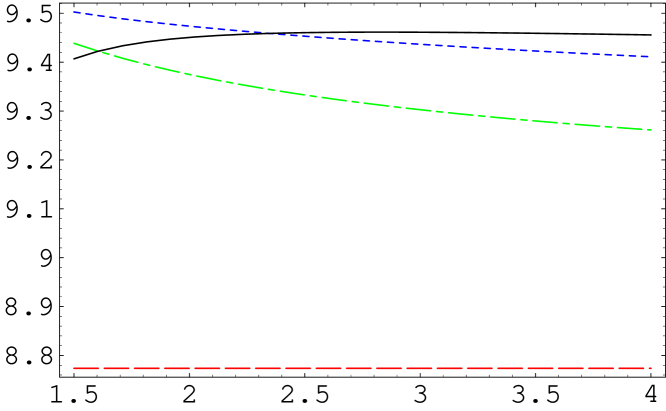
Figure 4: We plot $2m_{b,\rm RS}$ (dashed line), and the LO (dot-dashed line), NLO (dotted line) and NNLO (solid line) predictions for the $\Upsilon(1S)$ mass in terms of $\nu$ in the RS scheme. The value of $m_{b,\rm RS}$ is taken from Eq. (37).

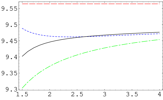
Figure 5: We plot $2m_{b,\rm RS^{\prime}}$ (dashed line), and the LO (dot-dashed line), NLO (dotted line) and NNLO (solid line) predictions for the $\Upsilon(1S)$ mass in terms of $\nu$ in the RS’ scheme. The value of $m_{b,\rm RS^{\prime}}$ is taken from Eq. (39).

We can also check the dependence of our results with respect to the theoretical and experimental parameters. As a first estimation of the errors, we allow for a variation of $\nu$, $\nu_{f}$, $\alpha_{s}$ and $N_{m}$ as follows: $\nu=2.5^{+1.5}_{-1}$ GeV, $\nu_{f}=2\pm 1$ GeV, $\alpha_{s}(M_{z})=0.118\pm 0.003$ and $N_{m}=0.552\pm 0.0552$. For the RS scheme, we obtain the following result

$$m_{b,\rm RS}(2\;{\rm GeV})=4\,387^{+2}_{+28}(\nu)^{-5}_{+7}(\nu_{f})^{-16}_{+16}(\alpha_{s})^{-68}_{+68}(N_{m})\;{\rm MeV};$$ (37)

$$m_{b,\overline{\rm MS}}(m_{b,\overline{\rm MS}})=4\,203^{+2}_{+25}(\nu)^{-5}_{+6}(\nu_{f})^{-28}_{+27}(\alpha_{s})^{-10}_{+10}(N_{m})\;{\rm MeV}.$$ (38)

For the RS’ scheme, we obtain the result (with the same variation of the parameters)

$$m_{b,\rm RS^{\prime}}(2\;{\rm GeV})=4\,782^{-08}_{+31}(\nu)^{-7}_{+3}(\nu_{f})^{+15}_{-12}(\alpha_{s})^{-28}_{+28}(N_{m})\;{\rm MeV};$$ (39)

$$m_{b,\overline{\rm MS}}(m_{b,\overline{\rm MS}})=4\,214^{-08}_{+28}(\nu)^{-6}_{+3}(\nu_{f})^{-25}_{+25}(\alpha_{s})^{-9}_{+9}(N_{m})\;{\rm MeV}.$$ (40)

The $\overline{\rm MS}$ mass result depends weakly on the variation of $\nu_{f}$ and $N_{m}$. For the latter it may seem surprising in view of the strong dependence of the RS mass but, to some extent, the variation of $N_{m}$ can be understood as a change of scheme.

With the results obtained in Eqs. (37) and (39), the expansion for the $\Upsilon(1S)$ mass would read in the RS scheme (see Eq. (36)):

$$M_{\Upsilon(1S)}=8\,774+559+120+7\;{\rm MeV},$$ (41)

and in the RS’ scheme:

$$M_{\Upsilon(1S)}=9\,564-158+56-2\;{\rm MeV}\,.$$ (42)

Both series seem to show convergence. Nevertheless, only in the RS’ scheme a more physical interpretation can be given where the leading order solution corresponds to the negative Coulomb binding energy (but we can see that this affects very little the determination of the $m_{\overline{\rm MS}}$ mass).

Naively, from Eqs. (41)-(42), one would be very optimistic about the errors. Nevertheless, let us try to go deeper into the error analysis. First, it may be not realistic to conclude from these results that the magnitude of the NNLO terms is of order of few MeV. The relative size between different orders will depend on the scale (as one can see in Figs. 4 and 5). The major problems come at small $\nu$ and we will discuss them later. Leaving them aside, for the RS’ scheme, the NNLO contributions remain quite small, whereas for RS scheme they can be of the order of $-50$ MeV for large values of $\nu$. Being even more conservative, one can split the NNLO contributions into the ones due to the singlet static potential ($+62$ MeV and $45$ MeV, with $\nu=2.5$ GeV, for the RS and RS’ scheme, respectively) and the relativistic ($-55$ MeV and $-47$ MeV, with $\nu=2.5$ GeV, for the RS and RS’ scheme, respectively) ones. Each of them happen to be of the order of 50 MeV with opposite signs. As far as the relativistic corrections is concerned, we can see that they are comfortably smaller than the $O(m\alpha_{s}^{2})$ leading term. For the correction due to the singlet static potential, convergence is also found in the RS scheme, whereas in the RS’ scheme the convergence is quite slow. In fact, this is due to the fact that the magnitude of the LO and NLO terms in the RS scheme is larger than in the RS’ scheme. Nevertheless, the discussion on the magnitude of the corrections due to the static potential is quite delicate since it strongly depends on the value of $\nu_{f}$ used. A closer look also shows that the main part of the scale dependence comes from the relativistic corrections, which become very important at small scales. Nevertheless, one can think of this scale dependence arising because of neglecting some higher order logs that, on theoretical grounds, we know anyway. The, $O(m_{\rm OS}\alpha_{s}^{5})$, NNNLO logs are known in the OS scheme [14] (see also [15, 16]). They may be considered to be of two different origen. Either those which can be minimized by choosing $\nu$ of the order of the inverse Bohr radius (for these an explicit expression can be found in Ref. [17]), or those related either to the hard $(\sim\ln{m}$), or to the ultrasoft scale $(\sim\ln{\nu_{us}}$). Therefore, the only piece of $A_{101}^{5,\rm OS}$ left unknown (although by far the most difficult one) is the log-independent one. For this, there exists, at least, a large $\beta_{0}$ determination [17, 18]. In order, this evaluation in the OS scheme to be useful, one has to change to the RS scheme, where the renormalon cancellation is explicit and the NNNLO correction is expected to be of natural size (note that one has to take into account the change from the pole mass to the RS mass in the expressions). Once a value for the log-independent term of $A_{101}^{5,\rm OS}$ is assumed (we will use the large $\beta_{0}$ result), one can compute $A_{101}^{5,\rm RS}$ without any further ambiguity and, thus, the complete NNNLO correction. We will use this result to give an estimate of the NNNLO corrections (and, therefore, further substantiate our previous discussion on the convergence of the series), and in order to study the scale dependence. Note that at this stage a dependence on $\nu_{us}$ appears. If we believe that the large $\beta_{0}$ approximation provides (numerically) a good estimate of, at least, the size of the renormalon contribution to the binding energy in the OS scheme, we could expect our determination to provide a rough estimate of higher order effects. We show our results in Figs. 6 and 7.

Let us first concentrate on the scale dependence. We first consider the result without the inclusion of the logs related to the hard/ultrasoft scale (being them of different physical origen). The results are the dot-dashed line in Figs. 6 and 7. At small scales, we see the typical oscillatory behavior between different orders in the perturbative expansion when the series ends to converge. For scales where the calculation is reliable, we see that the correction goes in the direction one would expect by choosing a somewhat smaller value for $\nu$ (and therefore closer to the scale $m_{\rm RS}C_{f}\alpha_{s}\sim 2$ GeV) in the NNLO evaluation. On the other hand, if we are concerned about the absolute size of the NNNLO corrections, what we can see is that, according to our estimate, they are small. We can now add the large logs associated to the hard and ultrasoft scale (we use Eq. (19) from Ref. [14]). They depend on $\nu_{us}$. We have chosen $\nu_{us}=1$ GeV. Our results correspond to the dot lines in Figs. 6 and 7. We see that the correction is relatively small (and it goes closer to the dot-dashed result when we increase $\nu_{us}$). It also blows up for small values of $\nu$ (this makes us believe that in order to properly deal with the scale dependence at small $\nu$ a renormalization-group improved evaluation could be useful). Therefore, we feel relatively confident about these sources of NNNLO corrections. However, this evaluation can not give an estimate of genuine $O(m_{\rm RS}\alpha_{s}^{5})$ corrections coming from other sources. We will discuss some of them right now as well as non-perturbative effects.

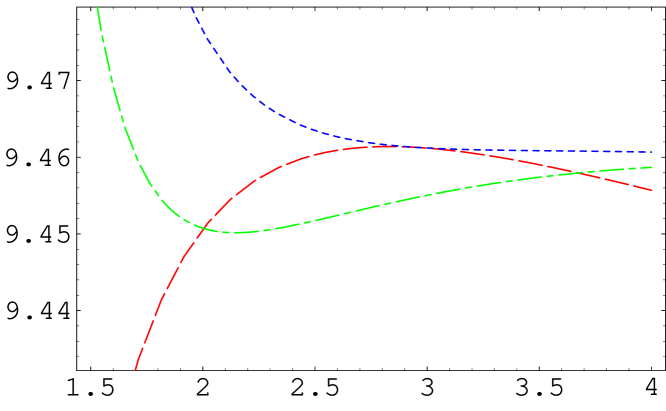
Figure 6: We plot the NNLO (dashed line) versus the NNNLO estimates in the RS scheme. a) NNNLO estimate without hard/ultrasoft logs (dot-dashed line) and b) NNNLO estimate including hard/ultrasoft logs with $\nu_{us}=1$ GeV (dotted line). The value of $m_{b,\rm RS}$ is taken from Eq. (37).

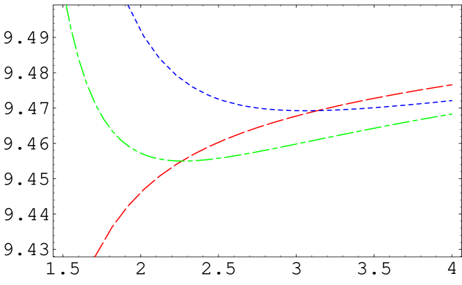
Figure 7: We plot the NNLO (dashed line) versus the NNNLO estimates in the RS’ scheme. a) NNNLO estimate without hard/ultrasoft logs (dot-dashed line) and b) NNNLO estimate including hard/ultrasoft logs with $\nu_{us}=1$ GeV (dotted line). The value of $m_{b,\rm RS^{\prime}}$ is taken from Eq. (39).

So far, we have just considered the expansion in $A_{nlj}^{n,\rm RS}\alpha_{s}^{n}$ and neglected the ultrasoft effects. Let us consider them now. An explicit expression for the leading correction due to ultrasoft effects can be obtained using the multipole expansion without any assumption about the perturbative or non-perturbative behavior at ultrasoft scales. It reads [41, 14] (we actually write the Euclidean expression for easier comparison with other results in the literature)

$$\delta M_{nlj}^{\rm US}(\nu_{us})\simeq\delta M_{nl}^{\rm US}(\nu_{us})={T_{F}\over 3N_{c}}\int_{0}^{\infty}\!\!dt\langle n,l|{\bf r}e^{-t(H_{o}^{\rm RS}-E_{n}^{\rm RS})}{\bf r}|n,l\rangle\langle g{\bf E}^{a}(t)\phi(t,0)^{\rm adj}_{ab}g{\bf E}^{b}(0)\rangle(\nu_{us}),$$ (43)

where $H_{o}^{\rm RS}\equiv\displaystyle{{\bf p}^{2}\over m_{\rm RS}}+{1\over 2N_{c}}{\alpha_{s}\over r}$ and $E_{n}^{\rm RS}\equiv-m_{\rm RS}C_{f}^{2}\alpha_{s}^{2}/(4n^{2})$. Different possibilities appear depending on the relative size of $\Lambda_{\rm QCD}$ with respect to the ultrasoft scale $m\alpha_{s}^{2}$. Let us first study whether the $\Upsilon(1S)$ lives in the situation where $\Lambda_{\rm QCD}\ll m\alpha_{s}^{2}$. In this case, the scale $m\alpha_{s}^{2}$ can be treated perturbatively and one can lowers further the cutoff up to the situation $\Lambda_{\rm QCD}\ll\nu^{\prime}_{us}\ll m\alpha_{s}^{2}$. Scales below $\nu^{\prime}_{us}$ can be parameterized in terms of local condensates within an expansion in $O({\Lambda_{\rm QCD}^{2}\over m^{2}\alpha_{s}^{4}})$. Eq. (43) would then read (with leading-log accuracy)

$$\delta M_{nl}^{\rm US}(\nu_{us})=\delta M_{nl}^{\rm US,\,pert.}+\delta M_{nl}^{\rm US,\,no-pert.}\,,$$ (44)

$$\delta M_{nl}^{\rm US,\,pert.} = E_{n}^{\rm RS}{\alpha_{s}^{3}\over\pi}\ln{\nu_{us}\over m_{\rm RS}\alpha_{s}}\left\{{C_{A}\over 3}\left[{C_{A}^{2}\over 2}+4C_{A}C_{f}{1\over n(2l+1)}+2C_{f}^{2}\left({8\over n(2l+1)}-{1\over n^{2}}\right)\right]\right.$$

$$\left.\qquad+{C_{f}^{2}\delta_{l0}\over 3n}8\left[C_{f}-{C_{A}\over 2}\right]\right\}\,,$$

and

$$\delta M_{nl}^{\rm US,\,no-pert.}=\sum_{n=0}^{\infty}C_{n}O_{n}\,,$$ (45)

where $C_{n}\sim 1/(m_{\rm RS}^{3+2n}\alpha_{s}^{4+4n})$ and $O_{n}\sim\Lambda_{\rm QCD}^{4+2n}$ (see [42] for details). $C_{0}O_{0}$ was first computed in Refs. [43] and $C_{1}O_{1}$ in Ref. [42]. The perturbative leading-log $\nu_{us}$ scale dependence would cancel against the scale dependence of $A_{10j}^{5,\rm RS}$ producing $\log(\alpha_{s})$-type terms. The validity of these results for the physical system under study rely on two assumptions that one should check. One the one hand, the final result will depend on $\alpha_{s}(m\alpha_{s}^{2})$ (this is easily seen within an effective field theory framework) but $m\alpha_{s}^{2}$ is an small scale for the $\Upsilon(1S)$. If we take as an estimate $\langle H_{o}-E_{1}\rangle_{10}\sim 360$ MeV, we see that perturbation theory is not truthsworthy for this scale (although, obviously, numerical factors can play a role). If one, anyway, wants to study this situation, one can include the log-dependent terms from Eq. (44) in the NNNLO perturbative estimate (the dependence on $\nu_{us}$ effectively disappears). This would produce a $\sim+50$ MeV shift in the RS scheme ($\sim+59$ MeV in the RS’ scheme) with respect to the NNLO results (for $\nu=2.5$ GeV), becoming even larger for small scales but decreasing for larger values of $\nu$ (in any case the shift depends on finite piece prescriptions) with, somewhat, the same shape than the dotted lines in Figs. 6 and 7. On the other hand, as far as the non-perturbative corrections is concerned, one should check that the operator product expansion in terms of local condensates converges. If we use our central values (in the RS’ scheme) plus the central values for the condensates used in Refs. [13, 42], we obtain

$$C_{0}O_{0}+C_{1}O_{1}=144-143\;{\rm MeV}\,.$$ (46)

We see that we do not find convergence. The situation improves by lowering the scale $\nu$ in $\alpha_{s}$ ($97-66$ MeV for $\nu=2$ GeV and $53-21$ MeV for $\nu=1.5$ GeV) and it also depends on the values of the condensates, which are poorly known. We see that this working hypothesis is not favored by the central set of parameters of the $\Upsilon(1S)$ system, although it can not be ruled out if one scan over the possible values of the parameters (in fact, if one considers $\nu=2$ GeV a more natural scale for the soft scale, the operator product expansion would be on the verge of convergence). Nevertheless, for $t$-$\bar{t}$ production near threshold, the situation $\Lambda_{\rm QCD}\ll m\alpha_{s}^{2}$ may be applicable and the results explained above useful.

It may then seem that the $\Upsilon(1S)$ system lives in the situation where $\Lambda_{\rm QCD}\sim m\alpha_{s}^{2}$. In that case, we can not lower further $\nu_{us}$ and the chromoelectric correlator in Eq. (43) cannot be computed using perturbation theory. We are then faced with the necessity of computing a non-perturbative non-local condensate. If in the previous case the knowledge of the local condensates was poor the situation is even worse now. This non-local condensate is related to the gluonic correlator for which the most general parameterization reads [44]

$$\langle gF_{\mu\nu}^{a}(x)\phi(x,0)^{\rm adj}_{ab}gF_{\rho\sigma}^{b}(0)\rangle = (\delta_{\mu\rho}\delta_{\nu\sigma}-\delta_{\mu\sigma}\delta_{\nu\rho})\left[{\cal D}(x^{2})+{\cal D}_{1}(x^{2})\right]$$ (47)

$$+ (x_{\nu}x_{\sigma}\delta_{\mu\rho}-x_{\nu}x_{\rho}\delta_{\mu\sigma}-x_{\mu}x_{\sigma}\delta_{\nu\rho}+x_{\mu}x_{\rho}\delta_{\nu\sigma}){\partial{\cal D}_{1}(x^{2})\over\partial x^{2}},$$

where for the gauge string a straight line is understood and ${\cal D}$ and ${\cal D}_{1}$ are invariant functions of $x^{2}$. In our case the following combination appears

$$\langle g{\bf E}^{a}(t)\phi(t,0)^{\rm adj}_{ab}g{\bf E}^{b}(0)\rangle=3\left({\cal D}(t^{2})+{\cal D}_{1}(t^{2})+t^{2}{\partial{\cal D}_{1}(t^{2})\over\partial t^{2}}\right).$$ (50)

In Ref. [47], a lattice evaluation of the gluonic correlator was performed. The following parameterization was used to describe the lattice data (with $t>0$)

$${\cal D}(t^{2})={b_{0}\over t^{4}}\exp{(-t/\lambda_{a})}+A_{0}\exp{(-t/\lambda_{A})}\qquad{\cal D}_{1}(t^{2})={b_{1}\over t^{4}}\exp{(-t/\lambda_{a})}+A_{1}\exp{(-t/\lambda_{A})}\,.$$ (51)

One would expect the $1/t^{4}$ terms to have something to do with the perturbative terms. In any case, at short distances, the gluonic correlator behavior should go closer to the one expected by perturbation theory. Unfortunately, we see no indication of this but rather the opposite. Whereas the perturbative result predicts a behavior $\sim-1/t^{4}$ for the $\langle{\bf E}(t)\cdot{\bf E}(0)\rangle$ operator, the lattice simulations get a positive slope at short distance (either for quenched or unquenched simulations). Lacking of any explanation for this fact, we will refrain of using those results in order to get an estimate of the non-perturbative effects (another point of concern is that the gluon condensate prediction for quenched simulations is one order of magnitude larger than the phenomenological value). Therefore, we will not try to give any number for the ultrasoft contribution in this paper and add them to the errors. In order not to overestimate them, we will constraint the allowed range of values for the ultrasoft contribution by some consistency arguments. If we rely on power counting rules, since $\Lambda_{\rm QCD}\sim m\alpha_{s}^{2}$, the non-perturbative effects would formally be of NNLO and from the discussion above about the perturbative NNLO effects one would assume a value around $\sim 50$ MeV. On the other hand, for consistency of the theory ($\Lambda_{\rm QCD}^{3}/(m\alpha_{s})^{2}\ll m\alpha_{s}^{2}$), the ultrasoft corrections should be smaller than the leading order solution (of order $\sim 160$ MeV). Note that if this consistency argument is not fulfilled, the very same assumption that we can describe, in first approximation, the $\Upsilon(1S)$ by a Coulomb-type bound state fails. In order to keep ourselves as conservative as possible, we would only demand the ultrasoft corrections to be smaller than the binding energy. Therefore, we will assign to our evaluation of the RS mass a $\pm 50$ MeV error. This is roughly equivalent to assign a $\pm 100$ MeV error to the evaluation of the binding energy from the ultrasoft contributions. This error may also be considered compatible with the discussion of the situation where $m\alpha_{s}^{2}\gg\Lambda_{\rm QCD}$. From the previous discussion about the magnitude of the NNNLO contributions, we will add another $\pm 25$ MeV error to our evaluation of the RS mass (roughly equivalent to assign a $\pm 50$ MeV error to the evaluation of the binding energy) from any other (perturbative) source of higher order effects. This may seem conservative in view of the estimates of the NNNLO effects shown in Figs. 6 and 7 and the related discussion but we also include the expected error from finite charm mass effects (see [18]). Therefore, from the RS scheme evaluation, our final estimate for the bottom mass reads (in order to avoid double counting with the error from higher order effects, we do not include now the scale dependence error)

$$m_{b,\rm RS}(2\;{\rm GeV})=4\,387^{+75}_{-75}({\rm US+higher\;orders})^{-16}_{+16}(\alpha_{s})^{-73}_{+75}(N_{m}+\nu_{f})\;{\rm MeV};$$ (52)

$$m_{b,\overline{\rm MS}}(m_{b,\overline{\rm MS}})=4\,203^{+67}_{-67}({\rm US+higher\;orders})^{-28}_{+27}(\alpha_{s})^{-15}_{+16}(N_{m}+\nu_{f})\;{\rm MeV}.$$ (53)

Whereas from the RS’ scheme evaluation, we obtain the result (with the same variation of the parameters)

$$m_{b,\rm RS^{\prime}}(2\;{\rm GeV})=4\,782^{+75}_{-75}({\rm US+higher\;orders})^{+15}_{-12}(\alpha_{s})^{-35}_{+31}(N_{m}+\nu_{f})\;{\rm MeV};$$ (54)

$$m_{b,\overline{\rm MS}}(m_{b,\overline{\rm MS}})=4\,214^{+67}_{-67}({\rm US+higher\;orders})^{-25}_{+25}(\alpha_{s})^{-15}_{+12}(N_{m}+\nu_{f})\;{\rm MeV}.$$ (55)

We average the two values obtained for the $\overline{\rm MS}$ mass. We then obtain (rounding)

$$m_{b,\overline{\rm MS}}(m_{b,\overline{\rm MS}})=4\,210^{+90}_{-90}({\rm theory})^{-25}_{+25}(\alpha_{s})\;{\rm MeV}\,,$$ (56)

where we have added (conservatively) the theoretical errors linearly. These figures compare favorably (within errors) with other determinations of the bottom mass. Either with other determinations using the $\Upsilon(1S)$ mass (the second references in [21, 52] and ref. [18]), sum rules [21, 18], lattice [48] or from measurements at LEP [49].

In this paper, we have just taken into account the first IR renormalon of the pole mass and the singlet static potential. Nevertheless, there are subdominant renormalons that eventually could play a role. On the singlet static potential side, one expects the first problems to come from a $O(\Lambda_{\rm QCD}^{3}r^{2})$ IR renormalon. For the pole mass there are $O(\Lambda_{\rm QCD}^{2}/m)$ renormalons. A priori, it is not clear which one will play the dominant role. In fact, it will depend on the relative size between $\Lambda_{\rm QCD}$ and $m\alpha_{s}^{2}$.

In the situation where a description in terms of local condensates is appropriated ($m\alpha_{s}^{2}\gg\Lambda_{\rm QCD}$), the leading genuine non-perturbative corrections to the mass scale like $m(\Lambda_{\rm QCD}/m\alpha_{s})^{4}$ but this quantity is (parametrically) much smaller than the non-perturbative effects associated to the subleading renormalons, either from the pole mass or from the singlet static potential. Moreover, in this case, parametrically, the leading ambiguity would come from the subleading pole mass renormalon of $O(\Lambda_{\rm QCD}^{2}/m)$. Therefore, we would be in a similar situation that when working with the pole mass, where the actual accuracy of the result was set by the perturbative calculation. Thus, one should first get rid of these subleading renormalons in order to improve the accuracy of the calculation before doing any reference about genuine non-perturbative effects.

In the situation where $m\alpha_{s}^{2}\sim\Lambda_{\rm QCD}$, the subleading renormalon ambiguities from the singlet static potential and the pole mass are parametrically of the same order than the genuine non-perturbative corrections. The $\Upsilon(1S)$ seems to live closer to this situation.

It is usually claimed that the non-perturbative effects in sum rules are smaller than in the $\Upsilon(1S)$ mass. We would like to mention that, at least parametrically, this is not the case under the standard counting ${1\over\sqrt{n}}\sim\alpha_{s}$ (where $n$ labels the moments in sum rules, see [20, 21] for details). Nevertheless, it may happen that they are numerically suppressed. This is indeed the case if one considers that one can describe the non-perturbative effects by local condensates [50]. However, one can only use the expression in terms of local condensates if one is in the situation where ${m\over n}\gg\Lambda_{\rm QCD}$. This would be analogous to the assumption $m\alpha_{s}^{2}\gg\Lambda_{\rm QCD}$ and it may difficult to fulfill. Therefore, it is more likely that the non-perturbative corrections will also depend on a nonlocal condensate, in fact, arising from the same effective theory, on the same chromoelectric correlator that the $\Upsilon(1S)$ mass does. Thus, in order to estimate the non-perturbative errors in sum rules evaluations, it would be most welcome to have, at least, the explicit expression of the non-perturbative effects in the situation ${m\over n}\sim\Lambda_{\rm QCD}$, which, by now, is lacking. In that way, one could relate the non-perturbative effects for different moments in the sum rules or with the non-perturbative effects of the $\Upsilon(1S)$ mass and eventually search for less sensitive non-perturbative physics observables.

6 Charm $\overline{\rm MS}$ quark mass determination

In this section, we give a determination of the $\overline{\rm MS}$ (and RS) charm mass. In principle, one could think of using the same procedure than in the previous section for the $J/\Psi$ (or $\eta_{c}$). This would imply to believe that the $J/\Psi$ is a mainly perturbative system. We prefer to avoid this assumption in this work and to obtain the charm mass in a different way. Our, maybe weaker, assumption will be to assume that HQET can be used for charm physics. We will search for observables that are weakly sensitive to non-perturbative physics. The observable that we will choose is the difference between the B and D meson mass. Here, it follows an analogous discussion than in the introduction. Whereas both the B meson mass and the D meson mass are $O(\Lambda_{\rm QCD})$ sensitive, the difference is $O(\Lambda_{\rm QCD}^{2}/m)$ sensitive. Nevertheless, this improvement is not exploited if one writes this observable in terms of the pole masses. Therefore, here, we will use the RS masses and our previous determination of the bottom mass in order to obtain the charm mass.

The (spin-averaged) mass difference between the B and D meson mass reads

$$\langle M_{B}\rangle-\langle M_{D}\rangle=m_{b,\rm RS}-m_{c,\rm RS}+\lambda_{1}\left({1\over 2m_{b,\rm RS}}-{1\over 2m_{c,\rm RS}}\right)+O(1/m_{\rm RS}^{2})\,,$$ (57)

where $\lambda_{1}$ can be related with the expectation value of the kinetic energy in HQET and

$$\langle M_{B(D)}\rangle={M_{B(D)}+3M_{B^{*}(D^{*})}\over 4}\,.$$ (58)

The value of $\lambda_{1}$ is poorly known. We take the value $\lambda_{1}=0.3\pm 0.2$ (see [51] and references therein). We can now obtain the value of the charm mass. We perform the evaluation in both schemes, the RS and RS’. In order to estimate the errors, we fix $\nu_{f}=1$ GeV and allow for a variation of $\alpha_{s}$, $N_{m}$, $\lambda_{1}$ and $m_{b}$ as follows: $\alpha_{s}(M_{z})=0.118\pm 0.003$, $N_{m}=0.552\pm 0.0552$, $\lambda_{1}=0.3\pm 0.2$ and $m_{b,\overline{\rm MS}}=4\,203^{+67}_{-67}$ MeV (in the RS scheme) and $m_{b,\overline{\rm MS}}=4\,214^{+67}_{-67}$ MeV (in the RS’ scheme). For the variation of $\alpha_{s}$ and $N_{m}$, we use the correlated values of the bottom mass (that is why we do not include these errors in the variation of the bottom mass). For the error due to $\nu_{f}$ see the discussion below. We obtain

$$m_{c,\rm RS}(1\;{\rm GeV})=1\,181^{+82}_{-84}(m_{b,\overline{\rm MS}})^{+4}_{-1}(\alpha_{s})^{-50}_{+50}(N_{m})^{-78}_{+65}(\lambda_{1})\;{\rm MeV};$$ (59)

$$m_{c,\overline{\rm MS}}(m_{c,\overline{\rm MS}})=1\,206^{+66}_{-67}(m_{b,\overline{\rm MS}})^{+1}_{-0}(\alpha_{s})^{+11}_{-13}(N_{m})^{-62}_{+52}(\lambda_{1})\;{\rm MeV},$$ (60)

and for the RS’ scheme

$$m_{c,\rm RS^{\prime}}(1\;{\rm GeV})=1\,477^{+79}_{-80}(m_{b,\overline{\rm MS}})^{+34}_{-27}(\alpha_{s})^{-19}_{+19}(N_{m})^{-54}_{+48}(\lambda_{1})\;{\rm MeV};$$ (61)

$$m_{c,\overline{\rm MS}}(m_{c,\overline{\rm MS}})=1\,207^{+65}_{-64}(m_{b,\overline{\rm MS}})^{-7}_{+5}(\alpha_{s})^{+13}_{-14}(N_{m})^{-43}_{+39}(\lambda_{1})\;{\rm MeV}.$$ (62)

We can check that the perturbative relation between the RS and $\overline{\rm MS}$ charm mass is indeed convergent. We obtain

$$m_{c,\rm RS}(1\;{\rm GeV}) = 1\,206-53+20+6+3=1\,181\;{\rm MeV},$$ (63)

$$m_{c,\rm RS^{\prime}}(1\;{\rm GeV}) = 1\,207+205+46+13+6=1\,477\;{\rm MeV}\,.$$

In order to test our evaluation, since, for the charm quark, $\nu_{f}$ stays close to the charm mass value (maybe jeopardizing the real structure of the perturbative expansion), we will also perform the calculation in the OS scheme (note that in that case large logs may appear). We use Eq. (57) with the replacement RS $\rightarrow$ OS. In order to achieve the renormalon cancellation, we rewrite both $m_{b,\rm OS}$ and $m_{c,\rm OS}$ in terms of the respective $\overline{\rm MS}$ masses and expand them in $\alpha_{s}(m_{c,\overline{\rm MS}})$. In this way, we obtain the renormalon cancellation for $m_{b,\rm OS}-m_{c,\rm OS}$ but not for the $1/m$ terms. Therefore, for the latter, we use the $\overline{\rm MS}$ masses as the expansion parameters. This effectively increases the magnitude of the $1/m$ terms but the other consistent option, to use the OS masses, is heavily affected by the renormalon (for instance $m_{c,\rm OS}=2\,263$ MeV for $m_{c,\overline{\rm MS}}=1\,210$ MeV) introducing even larger errors and not reflecting the real size of the $1/m$ corrections. We allow for the same variation of $\alpha_{s}$ and $\lambda_{1}$ than above, whereas for the bottom mass we use $m_{b,\overline{\rm MS}}=4\,210\pm 90$ MeV. We obtain

$$m_{c,\overline{\rm MS}}(m_{c,\overline{\rm MS}})=1\,254^{+85}_{-84}(m_{b,\overline{\rm MS}})^{+17}_{-12}(\alpha_{s})^{-49}_{+45}(\lambda_{1})\;{\rm MeV}\,.$$ (64)

We can check the convergence of the perturbative expansion of $m_{b,\rm OS}-m_{c,\rm OS}$ in terms of the $\overline{\rm MS}$ masses in order to test the validity of this evaluation. We obtain (order by order in $\alpha_{s}(m_{c,\overline{\rm MS}})$)

$$m_{b,\rm OS}-m_{c,\rm OS}=2\,956+490-14-32+22=3\,423\;{\rm MeV}\,.$$ (65)

For the last terms in the series the situation is not conclusive. One could think that the expansion is reliable up to, maybe, a $\sim\pm 30$ MeV uncertainty. One source of error comes from the expansion in $\alpha_{s}$ since two kind of logs arise: $\ln{(m_{b}/\nu)}$ and $\ln{(m_{c}/\nu)}$, which can not be minimized at the same time. In fact, for the choice $\nu=2m_{c,\overline{\rm MS}}$, we obtain $m_{c,\overline{\rm MS}}(m_{c,\overline{\rm MS}})=1\,239$ MeV and the expansion seems to improve:

$$m_{b,\rm OS}-m_{c,\rm OS}=2\,971+345+79+19+10=3\,424\;{\rm MeV}.$$

Let us consider further sources of error in the RS scheme evaluations. For these, we are using the RS bottom masses at a quite low $\nu_{f}=1$ GeV. This produces that the convergence in the conversion from the $\overline{\rm MS}$ to the RS and RS’ masses for the bottom quark is slower, in particular for the RS’ mass (see Table 4). One can then believe that higher orders in the relation between the $\overline{\rm MS}$ and the RS’ masses will add further positive contribution that in turn will increase the value of the $\overline{\rm MS}$ charm mass bringing it closer to the $\overline{\rm MS}$ evaluation. In any case, they are compatible within errors. Therefore, we add a $\pm 40(20)$ MeV error to our RS’(RS) evaluation from the conversion from the $\overline{\rm MS}$ to the RS’(RS) bottom quark mass. Another source of error comes from the $1/m$ terms. We have two effects compensating each other. With the RS scheme, the magnitude of the corrections in the relation between the RS and the $\overline{\rm MS}$ bottom quark mass is smaller but at the price of worsening the $1/m$ expansion (this observation could also apply to the OS calculation). With the RS’ scheme, the magnitude of the corrections in the relation between the RS and $\overline{\rm MS}$ bottom quark mass is larger but the $1/m$ expansion improves (as well as being less sensitive to $\lambda_{1}$). We estimate the $O(1/m^{2})$ corrections to be of order $\sim 15(30)$ MeV for the RS’(RS) evaluation and also add them to the errors. Overall, the theoretical errors in the RS and RS’ evaluations are basically equivalent. Therefore, we, somewhat, weigh more the RS’ scheme evaluation, being less sensitive to $\lambda_{1}$. Our final result for the $\overline{\rm MS}$ charm mass reads (rounding)

$$m_{c,\overline{\rm MS}}(m_{c,\overline{\rm MS}})=1\,210^{+70}_{-70}({\rm theory})^{+65}_{-65}(m_{b,\overline{\rm MS}})^{-45}_{+45}(\lambda_{1})\;{\rm MeV},$$ (66)

where we have not included the errors in $\alpha_{s}$ being negligible compared with the other sources of error. This result can be compared with two recent evaluations where Charmonium data was used [52].

At this stage, we can also give a prediction for $\bar{\Lambda}$ by using

$$\bar{\Lambda}_{\rm RS}=\langle M_{B}\rangle-m_{b,\rm RS}-{\lambda_{1}\over 2m_{b,\rm RS}}+O(1/m_{b,\rm RS}^{2})\,.$$ (67)

We obtain (using $m_{b,\overline{\rm MS}}=4\,210$ MeV)

$$\bar{\Lambda}_{\rm RS}(1\;{\rm GeV})=659\;{\rm MeV},\qquad\bar{\Lambda}_{\rm RS^{\prime}}(1\;{\rm GeV})=401\;{\rm MeV}.$$ (68)

We can see that it is crucial to specify the scheme in order to give a meaningful prediction for $\bar{\Lambda}$.

Finally, we would like to mention that $m_{b,\rm RS}-m_{c,\rm RS}$ (and $m_{b,\rm OS}-m_{c,\rm OS}$) suffers from renormalon ambiguities of $O(\Lambda_{\rm QCD}^{2}/m)$ that cancel with the renormalon of $\lambda_{1}/m$. Therefore, one could argue whether it makes any sense to give a value of $\lambda_{1}$ without specifying how to handle the $O(\Lambda_{\rm QCD}^{2}/m)$ renormalon in $m_{b,\rm RS}-m_{c,\rm RS}$. This could only be explained if the ambiguity due to the renormalon is much smaller than the genuine non-perturbative effects. If we take as an indication the perturbative expansions found above, we may believe that any ambiguity in the perturbative expansion is smaller than the genuine non-perturbative effects. On the other hand, this ambiguity may explain the spread of values one can find in the literature for $\lambda_{1}$.

7 Conclusions and outlook

We have approximately computed the normalization constant of the first infrared renormalon of the pole mass (and the singlet static potential). Estimates of the higher order coefficients of the perturbative series relating the pole mass with the $\overline{\rm MS}$ mass (and the singlet static potential with $\alpha_{s}$) have been obtained without relying on the large $\beta_{0}$ approximation. New, renormalon free, definitions of the mass and potential have been given, within an effective field theory perspective, by subtracting their closest singularities in the Borel plane. We have obtained the bottom $\overline{\rm MS}$ quark mass from the $\Upsilon(1S)$ mass, and an estimate of the errors, within this new scheme. We have also obtained the charm $\overline{\rm MS}$ mass by using the mass difference between the $B$ and $D$ mesons. Our final figures read

$$m_{b,\overline{\rm MS}}(m_{b,\overline{\rm MS}})=4\,210^{+90}_{-90}({\rm theory})^{-25}_{+25}(\alpha_{s})\;{\rm MeV}$$ (69)

and

$$m_{c,\overline{\rm MS}}(m_{c,\overline{\rm MS}})=1\,210^{+70}_{-70}({\rm theory})^{+65}_{-65}(m_{b,\overline{\rm MS}})^{-45}_{+45}(\lambda_{1})\>{\rm MeV}.$$ (70)

Several lines of research may follow from our results.

The use of conformal mapping could eventually lead to an improved convergent series in the evaluations of $N_{m}$ and $N_{V}$.

It would be interesting to apply the RS scheme to bottomonium sum rules or to $t$-$\bar{t}$ production near threshold and see how large the differences are with respect other determinations avaliable in the literature.

Our result for the bottom mass has been obtained in the zero mass charm approximation. Finite charm mass effects [18, 53] should be incorporated in future studies.

We have seen that our evaluation suffers from scale dependence for small $\nu$. At NNLO, the main source of scale dependence comes from the relativistic corrections. The incorporation of NNNLO effects does not seem to correct this fact. It may happen that a renormalization-group improved result could solve this problem. It is worth noting that there already exists one result in the OS scheme in the situation where $m\alpha_{s}^{2}\gg\Lambda_{\rm QCD}$ [16]. It would be desirable to have an independent evaluation within pNRQCD and without relying on the unequality $m\alpha_{s}^{2}\gg\Lambda_{\rm QCD}$. After that, one should transform the renormalization-group improved results from the OS to a renormalon free scheme. This, a priori, may not turn out to be completely trivial.

One of the (potentially) major source of errors in our evaluation of the bottom mass is the non-perturbative contribution. Any (reliable) determination of this contribution will have an immediate impact on our understanding of the theoretical errors. On the one hand, it would put on more solid basis our implicit assumption that the leading order solution corresponds to a Coulomb-type bound state and, once this is achieved, it would move the error estimates of the non-perturbative effects from a qualitative level to a quantitative one, (hopefully) bringing them down significantly. On the other hand, one may think of cross-checking our result with other determinations. The fact that the difference happens to be relatively tiny supports our believe that (perturbative and non-perturbative) higher order effects are indeed not very large. Alternatively, one may search for combinations of observables less sensitive to long distance physics effects in order to get a more accurate result for the masses.

Leaving aside theoretical errors, one may expect to bring down the errors associated to other parameters of the theory significantly (if one has a large enough set of observables) by using global fits.

Another issue that deserves further consideration is whether it is possible to develop a renormalon subtraction scheme completely within dimensional regularization (see the discussion at the beginning of sec. 4). This would provide a better understanding of the physical system and therefore the errors could be estimated in a more reliable way.

We expect to come back to these issues in the near future.

Acknowledgments

I thank K.G. Chetyrkin and A. Hoang for useful discussions and N. Brambilla and A. Vairo for showing me some of their pictures prior to publication.

References

- [1] M.B. Voloshin and M.A. Shifman, Sov. J. Nucl. Phys. 45, 292 (1987); H.D. Politzer and M.B. Wise, Phys. Lett. B206, 681 (1988); N. Isgur and M.B. Wise, Phys. Lett. B232, 113 (1989); E. Eichten and B. Hill, Phys. Lett. B234, 511 (1990); H. Georgi, Phys. Lett. B240, 447 (1990); B. Grinstein, Nucl. Phys. B339, 253 (1990).
- [2] W.E. Caswell and G.P. Lepage, Phys. Lett. B167, 437 (1986); G.T. Bodwin, E. Braaten and G.P. Lepage, Phys. Rev. D51, 1125 (1995); (E) ibid. D55, 5853 (1997).
- [3] A. Pineda and J. Soto, Nucl. Phys. B (Proc. Suppl.) 64, 428 (1998); Phys. Lett. B420, 391 (1998); Phys. Rev. D59, 016005 (1999).
- [4] N. Brambilla, A. Pineda, J. Soto and A. Vairo, Nucl. Phys. B566, 275 (2000).
- [5] M. Luke, A.V. Manohar and M.J. Savage, Phys. Rev. D 51, 4924 (1995).
- [6] M. Beneke, Phys. Rep. 317, 1 (1999).
- [7] M. Beneke and V. M. Braun, Nucl. Phys. B426, 301 (1994).
- [8] I. Bigi, M. Shifman, N. Uraltsev and A. Vainshtein, Phys. Rev. D50, 2234 (1994).
- [9] N. Gray, D.J. Broadhurst, W. Grafe and K. Schilcher, Z. Phys. C48, 673 (1990); K. Melnikov and T. van Ritbergen, Phys. Lett. B482, 99 (2000); K.G. Chetyrkin and M. Steinhauser, Nucl. Phys. B573 617 (2000).
- [10] W. Fischler, Nucl. Phys. B129, 157 (1977); Y. Schröder, Phys. Lett. B447, 321 (1999); M. Peter, Phys. Rev. Lett. 78, 602 (1997).
- [11] N. Brambilla, A. Pineda, J. Soto and A. Vairo, Phys. Rev. D60, 091502 (1999).
- [12] A. Pineda and J. Soto, Phys. Lett. B495, 323 (2000).
- [13] A. Pineda and F.J. Ynduráin, Phys. Rev. D58, 094022 (1998); ibid. D61, 077505 (2000); S. Titard and F.J. Ynduráin, Phys. Rev. D49, 6007 (1994).
- [14] N. Brambilla, A. Pineda, J. Soto and A. Vairo, Phys. Lett. B470, 215 (1999).
- [15] B.A. Kniehl and A.A. Penin, Nucl. Phys. B563, 200 (1999); ibid. B577, 197 (2000).
- [16] A.H. Hoang, A.V. Manohar and I.W. Stewart, hep-ph/0102257.
- [17] Y. Kiyo and Y. Sumino, Phys. Lett. B496, 83 (2000).
- [18] A.H. Hoang, hep-ph/0008102.
- [19] M. Beneke, A. Signer and V.A. Smirnov, Phys. Rev. Lett. 80, 2535 (1998); A. Czarnecki and K. Melnikov, Phys. Rev. Lett. 80, 2531 (1998).
- [20] A.H. Hoang, Phys. Rev. D59, 014039 (1999); A.A. Penin and A.A. Pivovarov, Nucl. Phys. B549, 217 (1999).
- [21] K. Melnikov and A. Yelkhovsky, Nucl. Phys. B528, 59 (1998); M. Beneke and A. Signer, Phys. Lett. B471, 233 (1999).
- [22] A.H. Hoang et al., Eur. Phys. J. direct C3, 1 (2000).
- [23] A.S. Kronfeld, Phys. Rev. D58, 051501 (1998).
- [24] M. Beneke, Phys. Lett. B344, 341 (1995).
- [25] T. Lee, Phys. Lett. B462, 1 (1999).
- [26] G. Cvetic and T. Lee, hep-ph/0101297.
- [27] M. Beneke and V.M. Braun, Phys. Lett. B348, 513 (1995); P. Ball, M. Beneke and V.M. Braun, Nucl. Phys. B452, 563 (1995).
- [28] K.G. Chetyrkin, B.A. Kniehl and A. Sirlin, Phys. Lett. B402, 359 (1997).
- [29] T. van Ritbergen, J.A.M. Vermaseren and S.A. Larin, Phys. Lett. B400, 379 (1997).
- [30] T. Appelquist, M. Dine and I. J. Muzinich, Phys. Rev. D17, 2074 (1978).
- [31] A. Pineda, PhD. thesis, Univ. Barcelona, January (1998); A.H. Hoang, M.C. Smith, T. Stelzer and S. Willenbrock, Phys. Rev. D59, 114014 (1999).
- [32] M. Beneke, Phys. Lett. B434, 115 (1998).
- [33] U. Aglietti and Z. Ligeti, Phys. Lett. B364, 75 (1995).
- [34] A.H. Hoang, Z. Ligeti and A.V. Manohar, Phys. Rev. Lett. 82, 277 (1999).
- [35] O. Yakovlev and S. Groote, Phys. Rev. D63, 074012 (2001).
- [36] T. Kinoshita and M. Nio, Phys. Rev. D53, 4909 (1996); P. Labelle, Phys. Rev. D58, 093013 (1998); B. Grinstein and I.Z. Rothstein, Phys. Rev. D57, 78 (1998); M. Luke and M.J. Savage, Phys. Rev. D57, 413 (1998).
- [37] A.V. Manohar, Phys. Rev. D56, 230 (1997); A. Pineda and J. Soto, Phys. Rev. D58, 114011 (1998).
- [38] M. Beneke and V.A. Smirnov, Nucl. Phys. B522, 321 (1998).
- [39] K.G. Chetyrkin, J.H. Kühn and M. Steinhauser, Comput. Phys. Commun. 133, 43 (2000).
- [40] M. Beneke, hep-ph/9911490.
- [41] M.B. Voloshin, Nucl. Phys. B154, 365 (1979).
- [42] A. Pineda, Nucl. Phys. B494, 213 (1997).
- [43] H. Leutwyler, Phys. Lett. B98, 447 (1981); M.B. Voloshin, Sov. J. Nucl. Phys. 36, 143 (1982).
- [44] H.G. Dosch and Yu A. Simonov, Phys. Lett. B205, 339 (1988).
- [45] Yu A. Simonov, Nucl. Phys. B324, 67 (1989).
- [46] I.I. Balitsky, Nucl. Phys. B254, 166 (1985).
- [47] A. Di Giacomo, E. Meggiolaro and H. Panagopoulos, Nucl. Phys. B483, 371 (1997); M. D’Elia, A. Di Giacomo and E. Meggiolaro, Phys. Lett. B408, 315 (1997).
- [48] V. Gimenez, L. Giusti, G. Martinelli and F. Rapuano, JHEP 0003, 018 (2000).
- [49] G. Rodrigo, A. Santamaria and M. Bilenkii, Phys. Rev. Lett. 79, 193 (1997).
- [50] M.B. Voloshin, Int. J. Mod. Phys. A10, 2865 (1995); A.I. Onishchenko, hep-ph/0005127.
- [51] M. Neubert, hep-ph/0001334.
- [52] M. Eidemuller and M. Jamin, Phys. Lett. B498, 203 (2001); N. Brambilla, Y. Sumino and A. Vairo, hep-ph/0101305.
- [53] M. Melles, Phys. Rev. D58, 114004 (1998); D. Eiras and J. Soto, Phys. Lett. B491, 101 (2000).