CERN-TH/2001-117

hep-ph/0104312

Neutrino Masses and Lepton Flavour Violation in
Thick Brane Scenarios

Gabriela Barenboim, G. C. Branco,^¶ André de Gouvêa, and M. N. Rebelo

Theory Division, CERN, CH-1211 Geneva 23, Switzerland.

We address the issue of lepton flavour violation and neutrino masses in the “fat-brane” paradigm, where flavour changing processes are suppressed by localising different fermion field wave-functions at different positions (in the extra dimensions) in a thick brane. We study the consequences of suppressing lepton number violating charged lepton decays within this scenario for lepton masses and mixing angles. In particular, we find that charged lepton mass matrices are constrained to be quasi-diagonal. We further consider whether the same paradigm can be used to naturally explain small Dirac neutrino masses by considering the existence of three right-handed neutrinos in the brane, and discuss the requirements to obtain phenomenologically viable neutrino masses and mixing angles. Finally, we examine models where neutrinos obtain a small Majorana mass by breaking lepton number in a far away brane and show that, if the fat-brane paradigm is the solution to the absence of lepton number violating charged lepton decays, such models predict, in the absence of flavour symmetries, that charged lepton flavour violation will be observed in the next round of rare muon/tau decay experiments.

1 Introduction

A few years ago, a new paradigm for addressing the gauge hierarchy problem was proposed [1]. In the so-called “large extra dimensions scenario,” (ADD scenario) the explanation for the large discrepancy between the weak scale and the Planck scale is that the fundamental scale of gravity is actually close to the weak scale, and that gravity seems weak to us because it propagates in more, compact, dimensions, while Standard Model fields are bound to four-dimensional subspaces embedded into the higher dimensional world.

One of the challenges for the ADD scenario is solving the well known problems of proton stability, absence of flavour changing neutral current processes, etc. The situation is particularly problematic because one has to consider nonrenormalizable operators which are only suppressed by powers of the “quantum gravity scale” and whose coefficients are completely unknown since they parametrise our ignorance concerning the physics above the ultraviolet cutoff. It is important to ask whether there are “low energy” mechanisms guaranteeing that most of these dangerous terms are appropriately suppressed, independently of the unknown beyond-quantum-field-theory physics.

A novel solution to the higher-dimensional flavour problems was proposed by Arkani-Hamed and Schmaltz [2] (AS scenario). They argue that if we live in a “fat” four-dimensional spacetime (fat brane), it is possible to effectively suppress unwanted higher dimensional operators by localising different fermion fields to different coordinates in the extra dimensions. As was also pointed out in [2], and further explored in [3, 4], this solution also provides an interesting explanation for the hierarchy of the quark masses and the values of the CKM mixing angles and CP-violating phase. It should be pointed that the AS scenario leads to startling consequences [5], which may be observed at next-generation collider experiments.

In this paper, we address the issue of lepton flavour violating phenomena in charged lepton decays and neutrino masses in the AS scenario. The AS scenario is natural for solving flavour changing problems, and indeed we find that it can very efficiently suppress charged lepton flavour violating decays such as $\mu,\tau\rightarrow l\gamma,lll$. One of the issues we explore here is whether suppressing such processes imposes any interesting constraint on lepton masses and mixing angles. We find, for example, that the charged lepton mass matrix is forced to be quasi-diagonal, and that almost all the mixing in the lepton sector must come from the neutral sector. Such a situation is certainly not observed in the quark sector (for an example, see [4]), and seems to already constrain some extra-dimensional neutrino mass scenarios.

The AS scenario also provides a natural mechanism for obtaining small Dirac neutrino masses, which has not yet been explored in the literature. It is important, therefore, to study whether similar success is obtained in explaining, for example, the large leptonic mixing angle which is required by neutrino oscillation solutions to the atmospheric neutrino puzzle [6]. We will show that in order to obtain large mixing angles, separations between different leptonic fields have to be closely related. The situation appears to be rather finely tuned when the flavour constraints mentioned above are also imposed.

The paper is organised as follows. In Sec. 2, we address the problem of flavour changing neutral currents in the ADD paradigm and how it is solved in the AS scenario. We concentrate on flavour violating charged lepton decays. In Sec. 3, we address the issue of lepton masses and mixing angles in a straightforward extension of the AS scenario, namely, adding right-handed neutrinos to the fat brane. We first discuss how “naturally” the AS scenario can explain the large hierarchies observed in the quark and fermion sectors, and what is required in order to obtain large mixing angles. We then analyse two-family models in great detail, concentrating on the constraints that must be met in order to obtain large mixing angles. Finally, we discuss solutions to the neutrino puzzles in the case of three generations. In Sec. 4, we discuss a mechanism for obtaining small neutrino masses without right-handed neutrinos. Here, constraints from the charged lepton sector severely restrict solutions to the neutrino puzzles. Our conclusions are presented in Sec. 5.

2 Lepton Flavour Violation and Large Extra Dimensions

It is a general principle of effective field theories that all operators consistent with the exact symmetries of Nature are present, including nonrenormalizable, “irrelevant” operators. These operators are understood as being suppressed by the large energy scale above which the effective field theory is no longer applicable. These include, for example, $(1/\Lambda^{2})QQQL$, which mediates proton decay and $(1/\Lambda)LHLH$, which breaks lepton number and gives the neutrinos a Majorana mass after electroweak symmetry breaking. It is also well known that $\Lambda$ is constrained to be at least of the order of the grand unification scale ($M_{GUT}\simeq 10^{16}$ GeV) by the fact that the proton lifetime is larger than $\sim 3\times 10^{33}$ years [7]. On the other hand, values of $\Lambda\sim 10^{9-14}$ GeV are required in order to correctly account for the atmospheric neutrino puzzle via neutrino oscillations.

In theories where the “quantum gravity” scale is small (a few TeV), one is faced with the challenge of explaining why, even though $\Lambda\sim 1$ TeV, phenomena which violate the conservation of “accidental” global symmetries have not been copiously observed. The two irrelevant operators mentioned above can be eliminated by assuming, for example, that (gauged) $B-L$ is a true symmetry of Nature (probably weakly broken, if one wants to explain the matter–antimatter asymmetry of the universe), but other dangerous operators still remain. These include operators that violate individual flavour number conservation and mediate phenomena such as meson–antimeson mixing and flavour changing neutral currents.

One intriguing solution to these problems was proposed by Arkani-Hamed and Schmaltz [2]. They postulate that the standard model fields are constrained to a “fat brane,” which is infinite in three space directions and occupies a finite volume in $n$ extra, orthogonal, compact dimensions. It is also postulated that gauge fields and the Higgs scalar can freely propagate in the entire volume of the fat brane, but fermions are confined to specific “points.” Finally, if one assumes that different fermion fields are located at different points in the extra dimensions, it is easy to see that some operators are “forbidden” by locality, e.g., an operator such as $(1/\Lambda^{2})QQQL$ can be very efficiently suppressed simply because $Q$’s and $L$’s live in different worlds, and don’t “see” one another [2].

In this section we discuss, within the scenario described above (AS scenario), what requirements are imposed on the distances between different leptonic fields in order to account for the (negative) experimental searches for charged lepton decays which violate lepton flavour number. Here we will concentrate on the lepton flavour violating muon decays

$$\mu\rightarrow e\gamma,\hskip 56.9055pt\mu\rightarrow eee,$$ (2.1)

and tau decays

$$\tau\rightarrow\mu\gamma,\hskip 28.45274pt\tau\rightarrow e\gamma,\hskip 28.45274pt\tau\rightarrow\mu\mu\mu,\hskip 28.45274pt\tau\rightarrow eee.$$ (2.2)

The process $l^{k}\rightarrow l^{l}\gamma$ ($k,l=\tau,\mu,e$) is mediated by the effective Lagrangian

$$-{\cal L}_{\l^{k}\rightarrow l^{l}\gamma}=\frac{a_{R}v}{\Lambda^{2}}\left(\bar{l^{k}_{L}}\sigma_{\mu\nu}l^{l}_{R}F^{\mu\nu}\right)+\frac{a_{L}v}{\Lambda^{2}}\left(\bar{l^{k}_{R}}\sigma_{\mu\nu}l^{l}_{L}F^{\mu\nu}\right)+h.c.,$$ (2.3)

after electroweak symmetry breaking. Here the subscript $L,R$ refers to the chirality, $F^{\mu\nu}$ is the electromagnetic field strength, $v$ is the Higgs vacuum expectation value, and $a_{R,L}$ are dimensionless couplings.

The process $l^{k}\rightarrow l^{l}l^{l}l^{l}$ is mediated by the effective Lagrangian (after Fiertz rearrangements)

$$-{\cal L}_{l^{k}\rightarrow l^{l}l^{l}l^{l}} = -{\cal L}_{\l^{k}\rightarrow l^{l}\gamma}+$$ (2.4)

$$+\frac{1}{\Lambda^{2}}\left[b_{1}(\bar{l^{k}_{R}}l^{l}_{L})(\bar{l^{l}_{R}}l^{l}_{L})+b_{2}(\bar{l^{k}_{L}}l^{l}_{R})(\bar{l^{l}_{L}}l^{l}_{R})+\right.$$

$$+b_{3}(\bar{l^{k}_{R}}\gamma_{\mu}l^{l}_{R})(\bar{l^{l}_{R}}\gamma^{\mu}l^{l}_{R})+b_{4}(\bar{l^{k}_{L}}\gamma_{\mu}l^{l}_{L})(\bar{l^{k}_{L}}\gamma^{\mu}l^{l}_{L})+$$

$$\left.+b_{5}(\bar{l^{k}_{R}}\gamma_{\mu}l^{l}_{R})(\bar{l^{l}_{L}}\gamma^{\mu}l^{l}_{L})+b_{6}(\bar{l^{k}_{L}}\gamma_{\mu}l^{l}_{L})(\bar{l^{l}_{R}}\gamma^{\mu}l^{l}_{R})+h.c.\right],$$

where $b$’s are dimensionless couplings. Eq. (2.3) mediates $l^{k}\rightarrow l^{l}l^{l}l^{l}$ by attaching an $l^{l}\bar{l^{l}}$ pair to the photon leg.

In the AS scenario, one can relate the constants $a,b$ to the distance between different leptonic fields and to higher dimensional couplings by integrating out the extra dimensions. One obtains, for example,

$$a_{R}\propto\alpha_{R}\int{\rm d}ye^{-\mu^{2}(y-l_{k})^{2}}e^{-\mu^{2}(y-e_{l})^{2}}\propto\alpha_{R}e^{-\frac{1}{2}\mu^{2}(l_{k}-e_{l})^{2}}$$ (2.5)

and

$$b_{4}\propto\beta_{4}\int{\rm d}ye^{-\mu^{2}(y-l_{k})^{2}}\left(e^{-\mu^{2}(y-l_{l})^{2}}\right)^{3}\propto\beta_{4}e^{-\frac{3}{4}\mu^{2}(l_{k}-l_{l})^{2}},$$ (2.6)

assuming one extra dimension and defining the higher-dimensional wave-function of the fermions to be Gaussians of width $\mu^{-1}/\sqrt{2}$ centred at position $l_{k,l}$ and $e_{k,l}$ for $l_{L}^{k,l}$ and $l_{R}^{k,l}$, respectively. The couplings $\alpha,\beta$ are dimensionless numbers, which are assumed to be of order one, since there is, a priori no reason for them to be either very small or very large. All $\alpha$ and $\beta$ will be, henceforth, set to unity unless otherwise noted.

From Eqs. (2.3,2.4) and assuming the AS scenario, it is easy to compute the branching ratios for the various lepton decays (see, for example, [8]) as a function of $\Lambda$ (the “quantum gravity” scale) and the distance between different lepton fields.

Fig. 1 depicts the branching ratio for $\mu\rightarrow e\gamma$ (right) and $\tau\rightarrow l\gamma$, $l=e,\mu$ (left) normalised by the branching ratio for $\mu\rightarrow e\nu\bar{\nu}$ and $\tau\rightarrow l\nu\bar{\nu}$ respectively, as a function of $\Delta L$. Two different values of the cutoff, $\Lambda=10$ TeV and 1 TeV, are shown (top and bottom, respectively). Here, $\Delta L$ is either $|l_{\mu}-e_{e}|$ or $|e_{\mu}-l_{e}|$ for the muon decay and $|l_{\tau}-e_{l}|$ or $|e_{\tau}-l_{l}|$ for the tau decay, in units of $\mu^{-1}$.

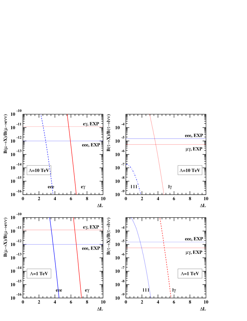
Figure 1: Branching ratio for $\mu\rightarrow X$ (right) and $\tau\rightarrow X$, (left) normalised by the branching ratio for $\mu\rightarrow e\nu\bar{\nu}$ and $\tau\rightarrow l\nu\bar{\nu}$ respectively, as a function of $\Delta L$, for two values of the quantum-gravity scale, $\Lambda=10$ GeV (top) and 1 GeV (bottom). See text for details. The horizontal lines indicate the current experimental constraints from searches for rare muon and tau decays [9]. In the case of tau decays, only the most and least stringent bounds are shown.

Fig. 1 also depicts the branching ratio for $\mu\rightarrow eee$ (right) and $\tau\rightarrow lll$, $l=e,\mu$ (left) normalised by the branching ratio for $\mu\rightarrow e\nu\bar{\nu}$ and $\tau\rightarrow l\nu\bar{\nu}$ respectively, as a function of $\Delta L$. Here, only nonzero $b_{3}$ and $b_{4}$ coefficients were considered. The reason for this is simple: given the requirements imposed by the non-observation of $\mu\rightarrow e\gamma$ and $\tau\rightarrow l\gamma$, the contribution of $a_{R,L},b_{1,2,5,6}$ are strongly suppressed, while $b_{3,4}$ are, a priori, unconstrained. Therefore, in this case, $\Delta L$ is either $|l_{\mu}-l_{e}|$ or $|e_{\mu}-e_{e}|$ for the muon decay and $|l_{\tau}-l_{l}|$ or $|e_{\tau}-e_{l}|$ for the tau decay, in units of $\mu^{-1}$.

Some comments are in order. First of all, it must be said that the AS scenario, as expected, is very efficient when it comes to suppressing rare lepton decays. Even for $\Lambda=1$ TeV, the most stringent requirement (from $\mu\rightarrow e\gamma$) is that $|l_{\mu}-e_{e}|,|l_{e}-e_{\mu}|\mathrel{\mathchoice{\lower 3.0pt\vbox{\halign{$\m@th\displaystyle\hfill#\hfil$\cr>\crcr\sim\crcr}}}{\lower 3.0pt\vbox{\halign{$\m@th\textstyle\hfill#\hfil$\cr>\crcr\sim\crcr}}}{\lower 3.0pt\vbox{\halign{$\m@th\scriptstyle\hfill#\hfil$\cr>\crcr\sim\crcr}}}{\lower 3.0pt\vbox{\halign{$\m@th\scriptscriptstyle\hfill#\hfil$\cr>\crcr\sim\crcr}}}}6.5\mu^{-1}$ (proton decay constraints require distances between quarks and lepton of order $10\mu^{-1}$ [2]). Second, one may wonder how strict the constraints are since, after all, there are order one coefficients floating about. It is easy to see that things do not change significantly if these coefficients are allowed to vary. For example, varying $\alpha_{R}$ from 0.3 to 3, the lower bound on $|\l_{\tau}-e_{\mu}|$ from $\tau\rightarrow\mu\gamma$ and $\Lambda=10$ TeV changes by $17\%$. A remaining question is what do these bounds imply for lepton masses and mixing angles. This will be addressed in the next sections.

Before proceeding, however, it is worthwhile mentioning at this point that other lepton flavour violating decays, such as $K\rightarrow\mu e$, hadronic tau decays and $\mu$–$e$ conversion in nuclei have not been considered, since they can be safely suppressed by assuming that quarks and leptons are well separated (which is generically required in order to suppress proton decay), and that the distance constraints obtained in these cases do not play a significant role when it comes to addressing lepton masses and mixing angles.

3 Right-Handed Neutrinos in the Brane

Another intriguing possibility is using the AS scenario to explain the current hierarchy of fermion masses and mixing angles [2]. Indeed, it has been shown that localising different quark fields to different points in the extra dimensions is an efficient and “natural” way of explaining not only all quark masses and mixing angles [3], but also the observed CP violation in the quark sector [4].

In this section, we study whether the same idea can be used to explain lepton masses. Charged lepton masses were already discussed in the context of massless neutrinos [3], but no similar study has been performed for neutrino masses.

The idea is quite simple. We assume the existence of three standard model singlet fermions, which we refer to as right-handed neutrinos ($N$), and assume that these are also localised at different points in the extra dimensions. If this is the case, neutrinos acquire ordinary Dirac masses after electroweak symmetry breaking, exactly like the quarks and charged leptons. In the AS scenario, the explanation for the smallness of the neutrino masses is straightforward: neutrino masses are tiny because $N$’s and $L$’s are separated by distances which are only slightly larger (as will become clear later) than, for example, the $Q$’s and $D$’s. It will turn out, as we will discuss in detail later, that the most serious challenge for the AS scenario with right-handed neutrinos in the brane will be to naturally account for the large mixing angles in the lepton sector which are required in order to solve the neutrino puzzles [6].

Before proceeding, it is worthwhile to digress a little on the philosophy behind the AS scenario when it comes to explaining fermion masses and mixing angles. Perhaps the most attractive, and certainly the novel idea behind the AS scenario is the possibility of solving the flavour problem without postulating new, horizontal symmetries. Instead, it is simply assumed that the fermions are separated by distances of a few (in units of the width of the fermionic higher dimensional wave-function $\mu^{-1}$), which could be chosen at random. All the work is done by the Gaussian suppression of the effective four dimensional Yukawa coupling (as discussed in the previous section. See also [2, 3]):

$$\lambda\propto e^{-\frac{1}{2}\mu^{2}(f_{i}-f_{j})^{2}},$$ (3.1)

where $f_{i}$ are the positions of the different fermion fields ($Q,U,D,L,E,N$).

In order to further quantify the “naturalness” concept, let us assume that, say, a $Q$ and a $U$ fields are localised in one extra dimension, of size $L\equiv 20\mu^{-1}$ (see [3] for a discussion on the expected size of $L\mu$). If the positions are chosen completely at random it is easy to show that the probability of finding $|q-u|\mu$ between some value $\delta$ and $\delta+{\rm d}\delta$ is given by $P(\delta){\rm d}\delta$, where

$$P(\delta)=0.1-.005\delta.$$ (3.2)

It is straightforward to compute the probability that the suppression due to the small overlap between the two extra dimensional wave-functions is of a given order of magnitude. Fig. 2 depicts the probability that the suppression factor is in some order of magnitude bin. It should be noted that while the figure only depicts suppression factors larger than $10^{-30}$, the probability that the suppression factor is smaller than $10^{-40}$ is almost 10%!

Figure 2: The probability for obtaining a suppression of the higher dimensional Yukawa coupling of a given order of magnitude. See text for details.

As expected, very tiny suppression factors can be obtained, even if all fields are constrained to lie relatively close to one another. An important fact is that, while random choices for the positions (in one extra dimension) seem to favour effective Yukawa coupling which are suppressed by an order of magnitude with respect to their higher dimensional counterparts, the probability of obtaining a large spread of suppression factors is quite large. It is this property which renders the AS solution to the fermion mass hierarchy attractive – random choices for the distances seem to provide a large spread for values of the Yukawa couplings, and therefore the observed hierarchies are naturally explained.

One can further pursue this logic and see what are the consequences for the mixing angles. We use a toy model of only two families of up-type quarks as an example, but it will become clear in due time that it is easily generalised to include three families and down-type quarks.

The mass matrix can be written as

$$M_{U}=\rho\left(\matrix{a&b\cr c&d}\right),$$ (3.3)

where $\rho$ is roughly the top quark mass and $a,b,c,d\leq 1$ are the suppression factors. The message from Fig. 2 is that, “normally” one expects $a\gg b\gg c\gg d$ (for example). If this is the case, one can trivially show that the matrix that diagonalizes $M_{U}M_{U}^{\dagger}$ is parametrised by one mixing angle, $\theta$, such that $\cos 2\theta=\pm 1\mp{\cal O}(c^{2}/a^{2},cbd/a^{3})$, i.e., $\theta$ is either close to 0 or $\pi/2$, such that the mixing is quite suppressed.

While this situation fits very nicely the quark masses and mixing angles, it poses serious problems for leptons, given that, according to the neutrino oscillation solution to the neutrino puzzles, at least one of the leptonic mixing angles is “large.” This is in sharp contrast to standard four dimensional approaches to the fermion mass puzzles. There, quark masses require a significant amount of underlying structure in order for one to understand the hierarchy of masses and the small mixing angles, while it has been argued that neutrino masses can be obtained from operators with random order one couplings [13]. The same is true in the case of the “simplest” neutrino mass model [14], where neutrino masses are obtained via the introduction of one single right-handed neutrino and the use of $1/M_{\rm Planck}$ operators.

In order to obtain large mixing angles, it is imperative that some elements of the mass matrices are of the same order. Using Eq. (3.3) as an example, it is again simple to show that, if one wants $\theta\simeq\pi/4$, $a\simeq c$ (for example) is required.

The challenge is, therefore, to obtain a mechanism satisfying this condition. Flavour symmetries, for example, would certainly do the job, but they would spoil the most attractive feature of the AS scenario. A different option, which still maintains the extra-dimensional nature of the AS scenario, is to assume that, as a consequence of the underlying localising mechanism, some fields are positioned on top of each other, and that some distances are, therefore, “naturally” very similar.

With this in mind, we proceed to discuss how realistic lepton masses and mixing angles can be obtained in the AS scenario. We first discuss the simpler two family case, and further address the issue of how “finely tuned” certain parameters have to be in order to obtain large mixing. Later, we discuss solutions for the more involved case of three families.

3.1 Two Neutrino Families

In this subsection we address in detail the case of only the two “heavy” lepton families, concentrating on the observed large mixing which seems to be required in the $\mu-\tau$ sector according to neutrino oscillation solutions to the atmospheric neutrino puzzle. It proves convenient to consider separately the different configurations which potentially yield maximal mixing in order to understand what constraints over the space of locations have to be met in order to obtain the appropriate mass-squared difference and mixing angle. These configurations are depicted in Fig. 3.

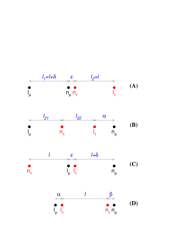
Figure 3: Different two family configurations which potentially lead to maximal mixing.

Two important comments concerning our discussion are in order. First, we assume that the order one coefficients which accompany the exponential suppressions (the higher dimensional Yukawa couplings) play no significant role, and set all of them to unity. We comment on the relevancy of this approximation later. Second, we impose that there is no significant mixing coming from the charged lepton sector. It turns out that, specially when considering only the $\mu-\tau$ sector, the non-observation of $\tau\rightarrow\mu\gamma$ combined with the requirement that the obtained $\tau$ mass agrees with the experimental value automatically forces the mixing in the charged lepton sector to be small. Note that the constraint of small mixing in the charged lepton sector will be considered a posteriori, and its consequences analysed for each of the different configurations.

By imposing the $\tau\rightarrow\mu\gamma$ constraint as discussed in the previous section, one obtains $|l_{\mu}-e_{\tau}|,|l_{\tau}-e_{\mu}|>3.73\mu^{-1}$ $(4.09\mu^{-1})$ for $\Lambda=10$ TeV (5 TeV), which in turn means that the off-diagonal elements of the (two generations) Dirac mass matrix for the charged leptons are less than (approximately) $\rho e^{-0.5(4)^{2}}=88$ MeV for $\rho=1.5\times m_{t}$, where $m_{t}\equiv 166$ GeV is the top quark mass (for details concerning the choice of $\rho$, see [3]). This, in turn, implies that one of the diagonal elements is necessarily of the order of the tau mass, while the other elements are at most of the order of the muon mass. In summary,

$$m_{l}\simeq m_{\tau}\left(\matrix{\epsilon(1+bc\epsilon)&b\epsilon\cr c\epsilon&1-\frac{\epsilon^{2}}{2}(b^{2}+c^{2})}\right),$$ (3.4)

where $b,c$ are numbers which are at most order one, $\epsilon\equiv m_{\mu}/m_{\tau}$, and $m_{\mu,\tau}$ are the muon and tau masses, respectively. Note that Eq. (3.4) is written in such a way that its eigenvalues are $m_{\mu}$ and $m_{\tau}$ up to $O(\epsilon^{2})$. In this case, it is easy to estimate the mixing angle, namely,

$$\sin^{2}\theta\simeq b^{2}\frac{m_{\mu}^{2}}{m_{\tau}^{2}}\mathrel{\mathchoice{\lower 3.0pt\vbox{\halign{$\m@th\displaystyle\hfill#\hfil$\cr<\crcr\sim\crcr}}}{\lower 3.0pt\vbox{\halign{$\m@th\textstyle\hfill#\hfil$\cr<\crcr\sim\crcr}}}{\lower 3.0pt\vbox{\halign{$\m@th\scriptstyle\hfill#\hfil$\cr<\crcr\sim\crcr}}}{\lower 3.0pt\vbox{\halign{$\m@th\scriptscriptstyle\hfill#\hfil$\cr<\crcr\sim\crcr}}}}10^{-3},$$ (3.5)

which is quite small.

A fact that will prove very important in the future is that, even though there is no direct significant limit on $|l_{\mu}-l_{\tau}|$ from $\tau\rightarrow\mu\mu\mu$ decays (see Fig. 1), it is geometrically constrained because $|l_{\tau}-e_{\tau}|<|l_{\mu}-e_{\tau}|$. It is easy to show that $|l_{\mu}-l_{\tau}|>|l_{\mu}-e_{\tau}|-|l_{\tau}-e_{\tau}|\simeq(4.0-3.14)\mu^{-1}$, independent of the number of extra dimensions. Therefore, as a guarantee that there are no large flavour changing effects in the charged lepton sector, a good rule of thumb is to keep $|l_{\mu}-l_{\tau}|\mathrel{\mathchoice{\lower 3.0pt\vbox{\halign{$\m@th\displaystyle\hfill#\hfil$\cr>\crcr\sim\crcr}}}{\lower 3.0pt\vbox{\halign{$\m@th\textstyle\hfill#\hfil$\cr>\crcr\sim\crcr}}}{\lower 3.0pt\vbox{\halign{$\m@th\scriptstyle\hfill#\hfil$\cr>\crcr\sim\crcr}}}{\lower 3.0pt\vbox{\halign{$\m@th\scriptscriptstyle\hfill#\hfil$\cr>\crcr\sim\crcr}}}}1\mu^{-1}$, in which case the mixing in the charged lepton sector is necessarily small.

Case A – Fig. 3(A) leads to the neutrino Dirac mass matrix

$$m_{\nu}=\rho\left(\matrix{e^{-\frac{\mu^{2}}{2}(l+\delta)^{2}}&e^{-\frac{\mu^{2}}{2}(l+\delta+\epsilon)^{2}}\cr e^{-\frac{\mu^{2}}{2}(l+\epsilon)^{2}}&e^{-\frac{\mu^{2}}{2}l^{2}}}\right),$$ (3.6)

where $l\equiv l_{2}$ and $\delta\equiv l_{1}-l_{2}$. We restrict ourselves to $\delta>0$, without loss of generality. As mentioned before, we will fix $\rho=1.5\times 166$ GeV.

It should be noted that the interchange of $n_{\mu}$ with $n_{\tau}$ (see Fig. 3) corresponds to a weak basis transformation which interchanges the two columns of $m_{\nu}$ but leaves $m_{\nu}m_{\nu}^{\dagger}$ unchanged. Note also that the configuration depicted in Fig. 3(A) leads automatically to very small mixing in the charged lepton sector, once the appropriate sizes for the neutrino masses are imposed.

Diagonalizing $m_{\nu}m_{\nu}^{\dagger}$ starting from Eq. (3.6) one obtains the mixing angle $\theta$, which, to a very good approximation (assuming $\delta,\epsilon\ll l$), is given by

$$\tan 2\theta\simeq\frac{2N_{1}(1+N_{2})}{(D_{1}-1)(D_{2}+1)},$$ (3.7)

where

$$N_{1} = \exp\left[-\frac{\mu^{2}}{2}(2l\delta+2l\epsilon+\delta^{2}+\epsilon^{2})\right],$$ (3.8)

$$N_{2} = \exp\left[-\mu^{2}\delta\epsilon\right],$$ (3.9)

$$D_{1} = \exp\left[-\mu^{2}(2l\delta+\delta^{2})\right],$$ (3.10)

$$D_{2} = \exp\left[-\mu^{2}(2l\epsilon+\epsilon^{2})\right].$$ (3.11)

The mass squared difference is

$$\Delta m^{2}=2\rho^{2}e^{-\mu^{2}l^{2}}N_{1}\left(1+N_{2}\right)\sqrt{1+\frac{1}{\tan^{2}2\theta}}.$$ (3.12)

Imposing large mixing, one can safely write

$$\Delta m^{2}\simeq 2\rho^{2}e^{-\mu^{2}l^{2}}N_{1}\left(1+N_{2}\right).$$ (3.13)

Note that in this approximation $\Delta m^{2}$ is equal to the numerator of $\tan 2\theta$ times $\rho^{2}e^{-\mu^{2}l^{2}}$. This important observation is valid in all cases we will discuss henceforth, as long as $\tan^{2}2\theta\gg 1$ (which is the condition we would like to meet).

We start by obtaining bounds for $l$. Since the largest element of $m_{\nu}$ is the (22) element, imposing an upper bound on the heaviest neutrino mass of $m^{2}\mathrel{\mathchoice{\lower 3.0pt\vbox{\halign{$\m@th\displaystyle\hfill#\hfil$\cr<\crcr\sim\crcr}}}{\lower 3.0pt\vbox{\halign{$\m@th\textstyle\hfill#\hfil$\cr<\crcr\sim\crcr}}}{\lower 3.0pt\vbox{\halign{$\m@th\scriptstyle\hfill#\hfil$\cr<\crcr\sim\crcr}}}{\lower 3.0pt\vbox{\halign{$\m@th\scriptscriptstyle\hfill#\hfil$\cr<\crcr\sim\crcr}}}}10$ eV² leads to $l>7.08\mu^{-1}$. On the other hand, from Eq. (3.13) and noting that $N_{1},N_{2}\leq 1$, one obtains a rough upper bound for $l$ by requiring $\Delta m^{2}>10^{-3}$ eV²: $l\mathrel{\mathchoice{\lower 3.0pt\vbox{\halign{$\m@th\displaystyle\hfill#\hfil$\cr<\crcr\sim\crcr}}}{\lower 3.0pt\vbox{\halign{$\m@th\textstyle\hfill#\hfil$\cr<\crcr\sim\crcr}}}{\lower 3.0pt\vbox{\halign{$\m@th\scriptstyle\hfill#\hfil$\cr<\crcr\sim\crcr}}}{\lower 3.0pt\vbox{\halign{$\m@th\scriptscriptstyle\hfill#\hfil$\cr<\crcr\sim\crcr}}}}7.8\mu^{-1}$. This can also be derived directly from Eq. (3.6) by noting that the largest neutrino mass matrix element should be (roughly) larger than the lower bound on $\sqrt{\Delta m^{2}}$ imposed by the atmospheric neutrino data. It is important to comment that for values of $\mu l$ close to the upper bound mentioned above, the neutrino masses are hierarchical, while for $\mu l$ much smaller than $7.7$, the eigenvalues of the neutrino mass matrix are degenerate and much larger than $\sqrt{\Delta m^{2}}$.

Next, we determine what values of $\epsilon$ and $\delta$, for fixed $l$, are required in order to obtain large mixing and the appropriate $\Delta m^{2}$ range. For fixed $l$, $\Delta m^{2}$ fixes the order of magnitude of $2N_{1}(1+N_{2})$ (see Eq. (3.13)), which is the numerator of $\tan 2\theta$ (see Eq. (3.7)). Large mixing requirements then determine the order of magnitude of $(D_{1}-1)$ (note that $D_{2}+1$ is $O(1)$), which allows one to compute an upper bound for $\delta$. Once this is done, one revisits the previous expressions and computes $\epsilon$. Table 1 contains values of $\mu\epsilon$ and $(\delta/l)_{max}$ as a function of $\mu l$.

Table 1: Case A – The allowed range of $\mu\epsilon$ and the maximum allowed value for $\delta/l$, for different values of $\mu l$, which satisfy $1\times 10^{-3}~{}{\rm eV^{2}}<\Delta m^{2}<8\times 10^{-3}~{}{\rm eV^{2}}$ and $|\tan 2\theta|>2.3$ [15].

$\mu l$	$\mu\epsilon$	$(\delta/l)_{\rm max}$
7.1	$\sim$ 1.1 – 1.3	$10^{-6}$
7.2	$\sim$ 0.9 – 1.2	$10^{-5}$
7.3	$\sim$ 0.7 – 1.0	$10^{-4}$
7.4	$\sim$ 0.5 – 0.8	$10^{-4}$
7.5	$\sim$ 0.3 – 0.6	$10^{-3}$
7.6	$\sim$ 0.1 – 0.4	$10^{-3}$
7.7	$\sim$ 0.0 – 0.2	$10^{-3}$

In order to examine how “finely-tuned” this scenario is, we look at the maximum value for the ratio $\delta/l$, which is how much the distance $|l_{\mu}-n_{\mu}|$ is allowed to deviate from $|l_{\tau}-n_{\tau}|$, normalised by the smallest distance. One can see that $(\delta/l)_{\rm max}\mathrel{\mathchoice{\lower 3.0pt\vbox{\halign{$\m@th\displaystyle\hfill#\hfil$\cr<\crcr\sim\crcr}}}{\lower 3.0pt\vbox{\halign{$\m@th\textstyle\hfill#\hfil$\cr<\crcr\sim\crcr}}}{\lower 3.0pt\vbox{\halign{$\m@th\scriptstyle\hfill#\hfil$\cr<\crcr\sim\crcr}}}{\lower 3.0pt\vbox{\halign{$\m@th\scriptscriptstyle\hfill#\hfil$\cr<\crcr\sim\crcr}}}}10^{-3}$ over all possible values of $l,\epsilon$, for small $\epsilon$. It is curious that the fine-tuning gets more severe as $\epsilon$ increases. This can be understood easily by the following line of reasoning: $\Delta m^{2}$ essentially constrains $\epsilon$ due to the fact that, it turns out, $\epsilon\gg\delta$; for small values of $l$, a large suppression is required in order to obtain the correct value for $\Delta m^{2}$, which must come from roughly $e^{-\mu^{2}l\epsilon}$. Hence bigger values of $\epsilon$ are required. However, larger values of $\epsilon$ suppress the numerator of Eq. (3.7), requiring a larger suppression in the denominator, which is mostly a function of $l$ and $\delta$, and the largest allowed value for $\delta$ decreases.

Case B – Fig. 3(B) leads to the Dirac mass matrix

$$m_{\nu}=\rho\left(\matrix{e^{-\frac{\mu^{2}}{2}(2l+\delta+\alpha)^{2}}&e^{-\frac{\mu^{2}}{2}l^{2}}\cr e^{-\frac{\mu^{2}}{2}\alpha^{2}}&e^{-\frac{\mu^{2}}{2}(l+\delta)^{2}}}\right),$$ (3.14)

where $l_{21}\equiv l$ and $\l_{22}\equiv l+\delta$. We first assume $\delta>0$. This leads, to a very good approximation (for $\delta\ll l$), to

$$\tan 2\theta\simeq\frac{2\exp\left[-\frac{\mu^{2}}{2}(2l^{2}+2l\delta+\delta^{2})\right]}{\exp[-\mu^{2}l^{2}]-\exp[-\mu^{2}\alpha^{2}]-\exp[-\mu^{2}(l+\delta)^{2}]},$$ (3.15)

and, remembering that we will require $\tan^{2}2\theta$ to be large,

$$\Delta m^{2}\simeq 2\rho^{2}\exp\left[-\frac{\mu^{2}}{2}(2l^{2}+2l\delta+\delta^{2})\right].$$ (3.16)

It is clear that the same approximate bounds on $l$, which applied in Case A, also apply here, and again we analyse what constraints are imposed on the other parameters for fixed values of $l$ within the allowed range. It should also be noted that, similarly to Case A, the charged lepton mass matrix is safely diagonal, given that, it turns out, $l_{21},l_{22}\mathrel{\mathchoice{\lower 3.0pt\vbox{\halign{$\m@th\displaystyle\hfill#\hfil$\cr>\crcr\sim\crcr}}}{\lower 3.0pt\vbox{\halign{$\m@th\textstyle\hfill#\hfil$\cr>\crcr\sim\crcr}}}{\lower 3.0pt\vbox{\halign{$\m@th\scriptstyle\hfill#\hfil$\cr>\crcr\sim\crcr}}}{\lower 3.0pt\vbox{\halign{$\m@th\scriptscriptstyle\hfill#\hfil$\cr>\crcr\sim\crcr}}}}7\mu^{-1}$.

For fixed $l$, the $\Delta m^{2}$ constraint fixes the range of $\delta$ and the numerator of $\tan 2\theta$ (Eq. (3.15)). The smallness of this term will determine how much the terms in the denominator of $\tan 2\theta$ are required to cancel in order to obtain large mixing. The only free parameter which remains is $\alpha$. Table 2 illustrates the severe fine-tuning between the value of $l$ and $\alpha$ which is required in order to obtain large mixing. Only for $l$ close to its upper bound is $\delta$ small enough to allow for a near perfect cancellation between the terms $e^{-\mu^{2}l^{2}}$ and $e^{-\mu^{2}(l+\delta)^{2}}$ in Eq. (3.15), in which case $\alpha$ plays no significant role, provided that $e^{-\mu^{2}\alpha^{2}}$ is small enough (which is satisfied for $\mu\alpha\mathrel{\mathchoice{\lower 3.0pt\vbox{\halign{$\m@th\displaystyle\hfill#\hfil$\cr>\crcr\sim\crcr}}}{\lower 3.0pt\vbox{\halign{$\m@th\textstyle\hfill#\hfil$\cr>\crcr\sim\crcr}}}{\lower 3.0pt\vbox{\halign{$\m@th\scriptstyle\hfill#\hfil$\cr>\crcr\sim\crcr}}}{\lower 3.0pt\vbox{\halign{$\m@th\scriptscriptstyle\hfill#\hfil$\cr>\crcr\sim\crcr}}}}7.8$). In this case, therefore, there is no need to tune the values of $\alpha$ and $l_{22}$ (this happens for $\mu l=7.7$ and $\mu\delta\mathrel{\mathchoice{\lower 3.0pt\vbox{\halign{$\m@th\displaystyle\hfill#\hfil$\cr<\crcr\sim\crcr}}}{\lower 3.0pt\vbox{\halign{$\m@th\textstyle\hfill#\hfil$\cr<\crcr\sim\crcr}}}{\lower 3.0pt\vbox{\halign{$\m@th\scriptstyle\hfill#\hfil$\cr<\crcr\sim\crcr}}}{\lower 3.0pt\vbox{\halign{$\m@th\scriptscriptstyle\hfill#\hfil$\cr<\crcr\sim\crcr}}}}0.05$). This does not mean, however, that there is no fine-tuning, since one is required to tune the values of $l_{21}$ and $l_{22}$ (for $\mu l=7.7$, $(\delta/l)_{\rm max}\mathrel{\mathchoice{\lower 3.0pt\vbox{\halign{$\m@th\displaystyle\hfill#\hfil$\cr<\crcr\sim\crcr}}}{\lower 3.0pt\vbox{\halign{$\m@th\textstyle\hfill#\hfil$\cr<\crcr\sim\crcr}}}{\lower 3.0pt\vbox{\halign{$\m@th\scriptstyle\hfill#\hfil$\cr<\crcr\sim\crcr}}}{\lower 3.0pt\vbox{\halign{$\m@th\scriptscriptstyle\hfill#\hfil$\cr<\crcr\sim\crcr}}}}10^{-3}$).

Table 2: Case B – The allowed range of $\mu\delta$ and the maximum allowed value for $|\alpha-l|/l$, for different values of $\mu l$, which satisfy $1\times 10^{-3}~{}{\rm eV^{2}}<\Delta m^{2}<8\times 10^{-3}~{}{\rm eV^{2}}$ and $|\tan 2\theta|>2.3$ [15].

$\mu l$	$\mu\delta$	$(|\alpha-l|/l)_{\rm max}$
7.1	$\sim$ 1.0 – 1.3	$10^{-6}$
7.2	$\sim$0.8 – 1.1	$10^{-5}$
7.3	$\sim$0.6 – 0.9	$10^{-5}$
7.4	$\sim$0.4 – 0.7	$10^{-4}$
7.5	$\sim$0.2 – 0.5	$10^{-3}$
7.6	$\sim$0.05 – 0.3	$10^{-2}$
7.7	$\sim$0.5 – 0.1	$10^{-2}$
	$\sim$0 – 0.05	unconstrained

Next, we examine the case $l_{21}>l_{22}$, i.e. $\delta<0$. In this case, the dominant term in the denominator of Eq. (3.15) is $e^{-\mu^{2}(l-|\delta|)^{2}}$, which cannot be cancelled by appropriately choosing $\alpha$. The only way to obtain large mixing is, therefore, to choose $|\delta|\ll l$ and $\alpha$ large. Numerically, we obtain that $\mu|\delta|$ cannot be larger than 0.05. The bounds on both $\Delta m^{2}$ and $\tan 2\theta$ can only be simultaneously satisfied for $\mu l_{22}=7.6$, $0.04\mathrel{\mathchoice{\lower 3.0pt\vbox{\halign{$\m@th\displaystyle\hfill#\hfil$\cr<\crcr\sim\crcr}}}{\lower 3.0pt\vbox{\halign{$\m@th\textstyle\hfill#\hfil$\cr<\crcr\sim\crcr}}}{\lower 3.0pt\vbox{\halign{$\m@th\scriptstyle\hfill#\hfil$\cr<\crcr\sim\crcr}}}{\lower 3.0pt\vbox{\halign{$\m@th\scriptscriptstyle\hfill#\hfil$\cr<\crcr\sim\crcr}}}}\mu|\delta|\mathrel{\mathchoice{\lower 3.0pt\vbox{\halign{$\m@th\displaystyle\hfill#\hfil$\cr<\crcr\sim\crcr}}}{\lower 3.0pt\vbox{\halign{$\m@th\textstyle\hfill#\hfil$\cr<\crcr\sim\crcr}}}{\lower 3.0pt\vbox{\halign{$\m@th\scriptstyle\hfill#\hfil$\cr<\crcr\sim\crcr}}}{\lower 3.0pt\vbox{\halign{$\m@th\scriptscriptstyle\hfill#\hfil$\cr<\crcr\sim\crcr}}}}0.05$ and $\mu l_{22}=7.7$ and $0\mathrel{\mathchoice{\lower 3.0pt\vbox{\halign{$\m@th\displaystyle\hfill#\hfil$\cr<\crcr\sim\crcr}}}{\lower 3.0pt\vbox{\halign{$\m@th\textstyle\hfill#\hfil$\cr<\crcr\sim\crcr}}}{\lower 3.0pt\vbox{\halign{$\m@th\scriptstyle\hfill#\hfil$\cr<\crcr\sim\crcr}}}{\lower 3.0pt\vbox{\halign{$\m@th\scriptscriptstyle\hfill#\hfil$\cr<\crcr\sim\crcr}}}}\mu|\delta|\mathrel{\mathchoice{\lower 3.0pt\vbox{\halign{$\m@th\displaystyle\hfill#\hfil$\cr<\crcr\sim\crcr}}}{\lower 3.0pt\vbox{\halign{$\m@th\textstyle\hfill#\hfil$\cr<\crcr\sim\crcr}}}{\lower 3.0pt\vbox{\halign{$\m@th\scriptstyle\hfill#\hfil$\cr<\crcr\sim\crcr}}}{\lower 3.0pt\vbox{\halign{$\m@th\scriptscriptstyle\hfill#\hfil$\cr<\crcr\sim\crcr}}}}0.05$, while $\mu\alpha\mathrel{\mathchoice{\lower 3.0pt\vbox{\halign{$\m@th\displaystyle\hfill#\hfil$\cr>\crcr\sim\crcr}}}{\lower 3.0pt\vbox{\halign{$\m@th\textstyle\hfill#\hfil$\cr>\crcr\sim\crcr}}}{\lower 3.0pt\vbox{\halign{$\m@th\scriptstyle\hfill#\hfil$\cr>\crcr\sim\crcr}}}{\lower 3.0pt\vbox{\halign{$\m@th\scriptscriptstyle\hfill#\hfil$\cr>\crcr\sim\crcr}}}}7.8$. In this case, the fine-tuning occurs between $l_{21}$ and $l_{22}$, which have to be equal to one another to more than one part in 10².

Case C – Fig. 3(C) leads to the Dirac mass matrix

$$m_{\nu}=\rho\left(\matrix{e^{-\frac{\mu^{2}}{2}(l+\delta+\epsilon)^{2}}&e^{-\frac{\mu^{2}}{2}l^{2}}\cr e^{-\frac{\mu^{2}}{2}(l+\delta)^{2}}&e^{-\frac{\mu^{2}}{2}(l+\epsilon)^{2}}}\right),$$ (3.17)

which yields the approximate relations ($\epsilon,\delta\ll l$)

$$\tan 2\theta\simeq\frac{2N^{\prime}_{1}[1+N^{\prime}_{2}]}{(1-D^{\prime}_{1})(1-D^{\prime}_{2})},$$ (3.18)

and

$$\Delta m^{2}\simeq 2\rho^{2}e^{-\mu^{2}l^{2}}N^{\prime}_{1}[1+N^{\prime}_{2}],$$ (3.19)

where

$$N^{\prime}_{1} = \exp\left[-\frac{\mu^{2}}{2}(2l\epsilon+\epsilon^{2})\right],$$ (3.20)

$$N^{\prime}_{2} = \exp\left[-\mu^{2}(2l\delta+\delta^{2}+\delta\epsilon)\right],$$ (3.21)

$$D^{\prime}_{1} = \exp\left[-\mu^{2}(2l\delta+\delta^{2})\right],$$ (3.22)

$$D^{\prime}_{2} = \exp\left[-\mu^{2}(2l\epsilon+\epsilon^{2})\right].$$ (3.23)

Note that the terms in the square bracket in Eqs. (3.18,3.19) are, by definition, between 1 and 2 and play no significant role in order of magnitude discussions. As in the two previous cases, $l$ is bound between roughly $7.1\mu^{-1}$ and $7.8\mu^{-1}$ (assuming the “atmospheric” $\Delta m^{2}$ and that $m_{\nu}^{2}<10$ eV²) and again we discuss the required cancellation among parameters for fixed values of $l$. As before, the requirement that $\Delta m^{2}$ satisfies the atmospheric neutrino data determines the order of magnitude of the numerator of $\tan 2\theta$ and, in this case, also determines the value of $\epsilon$. The requirement $|\tan 2\theta|>2.3$ is met by choosing $(1-D^{\prime}_{1})$ very small, which implies that $\delta$ has to be very small. Table 3 contains the value of $\mu l$, $\mu\epsilon$, and ($\delta/l)_{\rm max}$ which are obtained when trying to fit large mixing in the 2-3 sector with $\Delta m^{2}\sim 10^{-3}$ eV².

Table 3: Case C – The allowed range of $\mu\epsilon$ and the maximum allowed value for $\delta/l$, for different values of $\mu l$, which satisfy $1\times 10^{-3}~{}{\rm eV^{2}}<\Delta m^{2}<8\times 10^{-3}~{}{\rm eV^{2}}$ and $|\tan 2\theta|>2.3$ [15].

$\mu l$	$\mu\epsilon$	$(\delta/l)_{\rm max}$
7.1	$\sim$ 1.1 – 1.3	$10^{-6}$
7.2	$\sim$ 0.9 – 1.2	$10^{-5}$
7.3	$\sim$ 0.7 – 1.0	$10^{-4}$
7.4	$\sim$ 0.5 – 0.8	$10^{-4}$
7.5	$\sim$ 0.3 – 0.6	$10^{-3}$
7.6	$\sim$ 0.1 – 0.4	$10^{-3}$
7.7	$\sim$ 0.05 – 0.2	$10^{-1}$
	$\sim$ 0 – 0.05	unconstrained

It is noteworthy that in the limit $\epsilon\rightarrow 0$ there is no constraint on $\delta$. In this limit, the two lepton doublets are on top of each other, and large mixing is guaranteed, regardless of the location of the singlet fields. This situation, however, is in sharp contradiction with the bound from the flavour changing $\tau\rightarrow\mu\gamma$ decay, as discussed earlier in this section. Indeed, when we fit for the charged lepton masses imposing that $\tau\rightarrow\mu\gamma$ is small, we find that $\mu\epsilon\mathrel{\mathchoice{\lower 3.0pt\vbox{\halign{$\m@th\displaystyle\hfill#\hfil$\cr>\crcr\sim\crcr}}}{\lower 3.0pt\vbox{\halign{$\m@th\textstyle\hfill#\hfil$\cr>\crcr\sim\crcr}}}{\lower 3.0pt\vbox{\halign{$\m@th\scriptstyle\hfill#\hfil$\cr>\crcr\sim\crcr}}}{\lower 3.0pt\vbox{\halign{$\m@th\scriptscriptstyle\hfill#\hfil$\cr>\crcr\sim\crcr}}}}1$, and large mixing with the appropriate mass squared is only obtained for $\mu l\mathrel{\mathchoice{\lower 3.0pt\vbox{\halign{$\m@th\displaystyle\hfill#\hfil$\cr<\crcr\sim\crcr}}}{\lower 3.0pt\vbox{\halign{$\m@th\textstyle\hfill#\hfil$\cr<\crcr\sim\crcr}}}{\lower 3.0pt\vbox{\halign{$\m@th\scriptstyle\hfill#\hfil$\cr<\crcr\sim\crcr}}}{\lower 3.0pt\vbox{\halign{$\m@th\scriptscriptstyle\hfill#\hfil$\cr<\crcr\sim\crcr}}}}7.3$ (and $(\delta/l)_{\rm max}\mathrel{\mathchoice{\lower 3.0pt\vbox{\halign{$\m@th\displaystyle\hfill#\hfil$\cr<\crcr\sim\crcr}}}{\lower 3.0pt\vbox{\halign{$\m@th\textstyle\hfill#\hfil$\cr<\crcr\sim\crcr}}}{\lower 3.0pt\vbox{\halign{$\m@th\scriptstyle\hfill#\hfil$\cr<\crcr\sim\crcr}}}{\lower 3.0pt\vbox{\halign{$\m@th\scriptscriptstyle\hfill#\hfil$\cr<\crcr\sim\crcr}}}}10^{-5}$!).

Case D – Fig. 3(D) leads to the Dirac mass matrix

$$m_{\nu}=\rho\left(\matrix{e^{-\frac{\mu^{2}}{2}(l+\alpha+\beta)^{2}}&e^{-\frac{\mu^{2}}{2}(l+\alpha)^{2}}\cr e^{-\frac{\mu^{2}}{2}(l+\beta)^{2}}&e^{-\frac{\mu^{2}}{2}l^{2}}}\right),$$ (3.24)

which leads to the relations

$$\tan 2\theta=\frac{2N^{\prime\prime}_{1}[1+N^{\prime\prime}_{2}]}{(D^{\prime\prime}_{1}-1)(D^{\prime\prime}_{2}+1)-(1-e^{-2\mu^{2}\alpha\beta})D^{\prime\prime}_{1}D^{\prime\prime}_{2}},$$ (3.25)

and (for $\tan^{2}2\theta$ large)

$$\Delta m^{2}\simeq 2\rho^{2}e^{-\mu^{2}l^{2}}N^{\prime\prime}_{1}[1+N^{\prime\prime}_{2}],$$ (3.26)

where

$$N^{\prime\prime}_{1} = \exp\left[-\frac{\mu^{2}}{2}(2l\alpha+\alpha^{2})\right],$$ (3.27)

$$N^{\prime\prime}_{2} = \exp\left[-\mu^{2}(2l\beta+\beta^{2}+\alpha\beta)\right],$$ (3.28)

$$D^{\prime\prime}_{1} = \exp\left[-\mu^{2}(2l\alpha+\alpha^{2})\right],$$ (3.29)

$$D^{\prime\prime}_{2} = \exp\left[-\mu^{2}(2l\beta+\beta^{2})\right].$$ (3.30)

As in the previous cases, $\mu l$ is naively bound between $\sim[7.1,7.8]$ simply by requiring the largest neutrino mass squared to be less than 10 eV² and $\Delta m^{2}>10^{-3}$ eV². It is again useful to constrain the other parameters for fixed value of $\mu l$. In order to obtain a correct value for $\Delta m^{2}$, each value of $l$ requires a specific range of $\alpha$ (which determines $N^{\prime\prime}_{1}$, see Eq. (3.26)). Once $\alpha$ is fixed, we try to choose $\beta$ such that the mixing is large. In this case, however, it is easy to see that changing $\beta$ for fixed $\alpha$ and $l$ does very little to increase $\tan 2\theta$, as it mainly affects the value of $D^{\prime\prime}_{2}$, which plays a diminished role when it comes to determining the order of magnitude of $\tan 2\theta$ (see Eq. (3.25)).

The only possibility for obtaining large mixing is to choose $\alpha$ such that $(D^{\prime\prime}_{1}-1)$ is very small, i.e to choose $\alpha$ very small. Note that this choice automatically renders the term in the denominator of Eq. (3.25) proportional to $1-e^{2\mu^{2}\alpha\beta}$ small. Small values of $\alpha$ require $l$ to be large enough so that an appropriate value of $\Delta m^{2}$ is obtained. As a result, only values $\mu l\mathrel{\mathchoice{\lower 3.0pt\vbox{\halign{$\m@th\displaystyle\hfill#\hfil$\cr>\crcr\sim\crcr}}}{\lower 3.0pt\vbox{\halign{$\m@th\textstyle\hfill#\hfil$\cr>\crcr\sim\crcr}}}{\lower 3.0pt\vbox{\halign{$\m@th\scriptstyle\hfill#\hfil$\cr>\crcr\sim\crcr}}}{\lower 3.0pt\vbox{\halign{$\m@th\scriptscriptstyle\hfill#\hfil$\cr>\crcr\sim\crcr}}}}7.6,\mu\alpha\mathrel{\mathchoice{\lower 3.0pt\vbox{\halign{$\m@th\displaystyle\hfill#\hfil$\cr<\crcr\sim\crcr}}}{\lower 3.0pt\vbox{\halign{$\m@th\textstyle\hfill#\hfil$\cr<\crcr\sim\crcr}}}{\lower 3.0pt\vbox{\halign{$\m@th\scriptstyle\hfill#\hfil$\cr<\crcr\sim\crcr}}}{\lower 3.0pt\vbox{\halign{$\m@th\scriptscriptstyle\hfill#\hfil$\cr<\crcr\sim\crcr}}}}0.05$ potentially yield phenomenologically allowed values for $\Delta m^{2}$ and $\tan 2\theta$.

As in Case C, the charged lepton sector imposes (here very severe) constraints over the allowed values for the $|l_{\mu}-l_{\tau}|$ distance, $\alpha$. As discussed in the beginning of this subsection, $\mu\alpha\mathrel{\mathchoice{\lower 3.0pt\vbox{\halign{$\m@th\displaystyle\hfill#\hfil$\cr>\crcr\sim\crcr}}}{\lower 3.0pt\vbox{\halign{$\m@th\textstyle\hfill#\hfil$\cr>\crcr\sim\crcr}}}{\lower 3.0pt\vbox{\halign{$\m@th\scriptstyle\hfill#\hfil$\cr>\crcr\sim\crcr}}}{\lower 3.0pt\vbox{\halign{$\m@th\scriptscriptstyle\hfill#\hfil$\cr>\crcr\sim\crcr}}}}1$ is required by $\tau\rightarrow\mu\gamma$ constraints, which implies that there are no solutions with $10^{-3}~{}{\rm eV^{2}}<\Delta m^{2}<8\times 10^{-3}$ eV², $(m_{\nu}^{2})_{\rm max}<10$ eV², and $|\tan 2\theta|\geq 2.3$.

In summary, we have analysed in detail the issue of obtaining large mixing and $10^{-3}~{}{\rm eV^{2}}<\Delta m^{2}<8\times 10^{-3}$ eV² in the $\mu-\tau$ sector. For all configurations we discussed, this is only achieved by carefully choosing the value of specific distances. Quantitatively, we find that it is necessary that the value of two a priori independent distances be equal to, at least, 1 part in 10² in order to obtain large mixing in the atmospheric neutrino sector. Cases where maximum mixing is “naturally” obtained by placing fields “on top” of one another (Cases C and D), were ruled out by flavour changing neutral current constraints combined with obtaining the observed values for the corresponding charged lepton masses.

We conclude with a comment on the order one higher dimensional Yukawa couplings which we set to unity throughout. Firstly, note that these coefficients can be readily “absorbed” by slightly modifying the distance between the lepton fields. Explicitly,

$$\alpha e^{-\frac{\mu^{2}}{2}l^{2}} = e^{-\frac{\mu^{2}}{2}(l^{\prime})^{2}},$$ (3.31)

$$2\ln{\alpha}-(\mu l)^{2} = -(\mu l^{\prime})^{2},$$ (3.32)

$$\frac{l}{l^{\prime}} = \sqrt{1+\frac{2\ln{\alpha}}{(\mu l^{\prime})^{2}}},$$ (3.33)

where $l/l^{\prime}$ is how much the distance has to be changed in order to “absorb” the coefficient $\alpha$. For neutrino masses, $(\mu l^{\prime})^{2}\mathrel{\mathchoice{\lower 3.0pt\vbox{\halign{$\m@th\displaystyle\hfill#\hfil$\cr>\crcr\sim\crcr}}}{\lower 3.0pt\vbox{\halign{$\m@th\textstyle\hfill#\hfil$\cr>\crcr\sim\crcr}}}{\lower 3.0pt\vbox{\halign{$\m@th\scriptstyle\hfill#\hfil$\cr>\crcr\sim\crcr}}}{\lower 3.0pt\vbox{\halign{$\m@th\scriptscriptstyle\hfill#\hfil$\cr>\crcr\sim\crcr}}}}50$, such that, even if $\alpha$ were as small as 0.1, $|l/l^{\prime}-1|\mathrel{\mathchoice{\lower 3.0pt\vbox{\halign{$\m@th\displaystyle\hfill#\hfil$\cr<\crcr\sim\crcr}}}{\lower 3.0pt\vbox{\halign{$\m@th\textstyle\hfill#\hfil$\cr<\crcr\sim\crcr}}}{\lower 3.0pt\vbox{\halign{$\m@th\scriptstyle\hfill#\hfil$\cr<\crcr\sim\crcr}}}{\lower 3.0pt\vbox{\halign{$\m@th\scriptscriptstyle\hfill#\hfil$\cr<\crcr\sim\crcr}}}}0.05$. Secondly, and most importantly, the presence of the order one coefficients will not affect our fine-tuning discussions – parameters just have to be slightly “redefined.” For example, in Case A, instead of having to “tune” $l_{1}$ to $l_{2}$, one would tune $l_{1}$ to $l_{2}$ plus a small, constant, coefficient dependent on the ratio of the higher dimensional Yukawa couplings. The “amount” of fine-tuning remains the same.

3.2 Three Neutrino Families

In this subsection, we discuss the case of three lepton families, concentrating on obtaining appropriate neutrino mass-squared differences and mixing angles for solving the atmospheric and solar neutrino puzzles, while satisfying the constraints from the CHOOZ and Palo Verde experiments [16].

Unlike the two-family case, in the case of three families it is not simple to perform a search for all configurations which potentially yield the appropriate values for the oscillation parameters. Furthermore, after some configurations are identified, a general analytic discussion of “fine-tuning” among different parameters is not illuminating. For these reasons, we decided to approach the situation in a different way.

Initially, we numerically scanned the “location space” of the left-handed lepton doublets and the right-handed neutrino singlets, restricting ourselves to branes which are fat in only one extra dimension. During the scan, we looked for solutions which yield neutrino masses and mixing angles such that all the neutrino experimental data could be accounted for by neutrino oscillations [6]. Details of the numerical scan are described in the Appendix, and some results are the following: i- As expected, obtaining reasonable values for the mixing angles is quite hard, more so than the correct order of magnitude for the mass-squared differences. ii- In all of the acceptable configurations, the $\mu$–$\tau$ system falls into one of the configurations (see Fig. 3) discussed in detail in the previous subsection, with the same fine-tuning characteristics. iii- Only configurations which yield hierarchical neutrino masses were found. iv- For a significant fraction of the points ($\sim$50%) flavour changing effects in the charged lepton sector are absent, and the charged lepton mass matrix is virtually diagonal. In summary, it was possible to find several configurations which yield appropriate neutrino masses and mixing angles for explaining all neutrino data.

Four different configurations are depicted in Fig. 4. These are labelled PLMA, PSMA, PLOW and PVAC, alluding to the fact that they will fall into the LMA, SMA, LOW and VAC solutions [6] to the solar neutrino puzzle, respectively. Table 4 contains the exact distances for the four configurations. Note that PLMA and PVAC have the second and third generation configuration depicted in Fig. 3(B), while PSMA and PLOW present that depicted in Fig. 3(A).

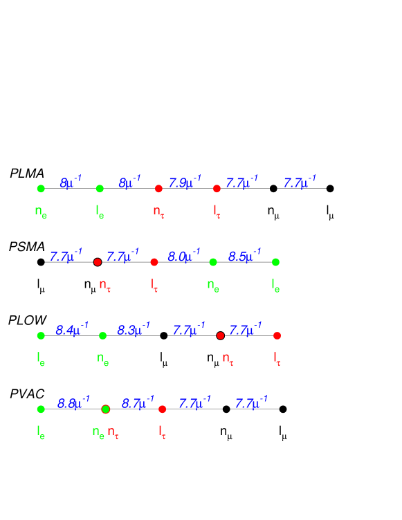
Figure 4: Four examples which yield neutrino masses and mixing angles which satisfy all neutrino data.

Table 4: Points which yield neutrino masses and mixing angles such that all neutrino data can be accommodated. The different points fall (PLMA, PSMA, PLOW, PVAC) in different solutions to the solar neutrino puzzle, and are labelled accordingly. For the definition of the parameters $l_{1},l_{2},l_{3},x,y$, see Fig. 8 in the Appendix.

configuration	$\mu l_{1}$	$\mu l_{2}$	$\mu l_{3}$	$\mu x$	$\mu y$
PLMA	8.0	-7.7	7.9	-16.0	-15.6
PSMA	8.5	7.7	7.7	15.7	0.0
PLOW	-8.4	7.7	7.7	-16.0	0.0
PVAC	-8.8	-7.7	8.7	0.0	-16.4

In order to try to quantify if/how these solutions are finely-tuned, we study the stability of the four configurations depicted in Fig. 4 by probing “around” them. Explicitly, we fix the “smallest” parameter ( $l_{2}$ in the case of PSMA and PLOW and $l_{3}$ in the case of PSMA and PLOW) and vary the other ones ($l_{1},x,y,$ and $l_{2}$ or $l_{3}$) from $p_{i}-0.1$ to $p_{i}+0.1$ in steps of 0.02, where $p_{i}$ is the original value of each of the four parameters (for a total of 11⁴ points). The size of the interval is guided by the results of our two-generation studies in the previous subsection, i.e., we choose an interval which is small enough so that the large atmospheric angle is not disturbed too much.

Fig. 5 (Fig. 6) depicts the result of this stability study around PLMA (PSMA). In the figures, we plot the values obtained for all the oscillation parameters: $\Delta m^{2}_{\rm atm}\times\tan^{2}\theta_{\rm atm}$ (top left), $\Delta m^{2}_{\rm atm}\times|U_{e3}|^{2}$ (top right), and $\Delta m^{2}_{\odot}\times\tan^{2}\theta_{\odot}$ (bottom). The thin [blue] boxes mark the “allowed regions,” as defined in the Appendix, while the solid, dark dot indicates the results obtained for PLMA (PSMA). When perturbing about PLOW and PVAC, similar results are obtained (indeed, we have repeated this procedure for a large number of points).

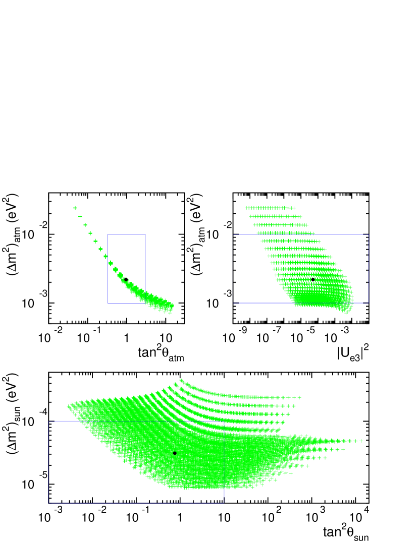
Figure 5: Values of $\Delta m^{2}_{\rm atm}\times\tan^{2}\theta_{\rm atm}$ (top, left), $\Delta m^{2}_{\rm atm}\times|U_{e3}|^{2}$ (top right), and $\Delta m^{2}_{\odot}\times\tan^{2}\theta_{\odot}$ (bottom) which are obtained when perturbing around PLMA (see text for details). The results obtained at PLMA is indicated by a solid, dark dot.

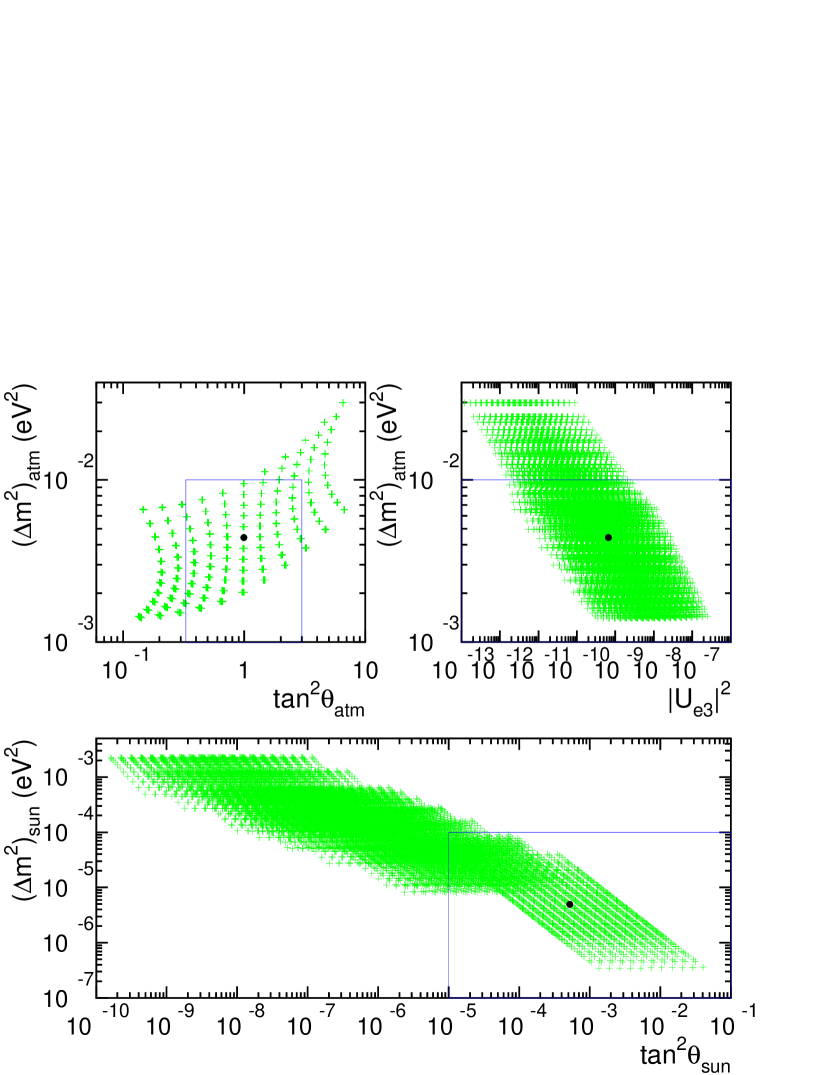
Figure 6: Same as Fig. 5, when perturbing around PSMA.

The results contained in the figure are quite interesting. First, it should be noted that, as expected, the atmospheric parameters do not vary substantially. Numerically, 56% (54%) of the points remain inside the “atmospheric box”, $10^{-3}~{}{\rm eV^{2}}<\Delta m^{2}_{\rm atm}<10^{-2}~{}{\rm eV^{2}}$, $1/3<\tan^{2}\theta_{\rm atm}<3$ in the case of PLMA (PSMA). On the other hand, some of the solar parameters and $|U_{e3}|^{2}$ vary drastically. For example, while perturbing around PLMA (PSMA), $\tan^{2}\theta_{\odot}$ varies by 7 (9) orders of magnitude, and similar results apply to $|U_{e3}|^{2}$. Moreover, $\Delta m^{2}_{\odot}$, while somewhat stable around PLMA (it varies by 2 orders of magnitude), spans 5 orders of magnitude around PSMA.

Does this observed numerical instability indicate a fine-tuning among different parameters? After all, what we would like to learn from these “stability studies” is whether, in order to guarantee that the solar parameters and $|U_{e3}|^{2}$ are inside a certain range, the distances between some lepton fields have to be chosen very carefully, and whether slight modifications severely spoil the result. In order to verify that this is the case, we look at PLMA and PSMA in more detail. The PLMA-like configurations (see Fig. 4) lead to the following neutrino Dirac mass matrix:

$$m_{\nu}=\left(\matrix{a&0&a^{\prime}\cr 0&b&0\cr 0&b^{\prime}&c}\right),$$ (3.34)

where $a,a^{\prime},b,b^{\prime},c$ are related, respectively, to the distances $|l_{e}-n_{e}|$, $|l_{e}-n_{\tau}|$, $|l_{\mu}-n_{\mu}|$, $|l_{\tau}-n_{\mu}|$, $|l_{\tau}-n_{\tau}|$. Eq. (3.34) leads to

$$m_{\nu}m_{\nu}^{\dagger}=\left(\matrix{a^{2}+a^{\prime 2}&0&a^{\prime}c\cr 0&b^{2}&bb^{\prime}\cr a^{\prime}c&bb^{\prime}&b^{\prime 2}+c^{2}}\right).$$ (3.35)

From the discussion in the previous subsection, we know that large mixing in the atmospheric sector is obtained for $b\simeq b^{\prime}>c$ (Case B). It is also easy to see that, in order to obtain $\Delta m^{2}_{\odot}<\Delta m^{2}_{\rm atm}$, $a,a^{\prime},c<b,b^{\prime}$. In light of this, we multiply Eq. (3.35) by a $\theta$ rotation about the “$e$-axis” such that $\sin{\theta}\equiv b^{\prime}/\sqrt{b^{2}+b^{\prime 2}}$ and obtain

$$\left(\matrix{1&0&0\cr 0&\cos\theta&\sin\theta\cr 0&-\sin\theta&\cos\theta}\right)\left(\matrix{a^{2}+a^{\prime 2}&0&a^{\prime}c\cr 0&b^{2}&bb^{\prime}\cr a^{\prime}c&bb^{\prime}&b^{\prime 2}+c^{2}}\right)\left(\matrix{1&0&0\cr 0&\cos\theta&-\sin\theta\cr 0&\sin\theta&\cos\theta}\right)\simeq$$

$$\left(\matrix{a^{2}+a^{\prime 2}&a^{\prime}c\sin\theta&a^{\prime}c\cos\theta\cr a^{\prime}c\sin\theta&b^{2}+b^{\prime 2}+c^{2}\sin^{2}\theta&c^{2}\sin\theta\cos\theta\cr a^{\prime}c\cos\theta&c^{2}\sin\theta\cos\theta&c^{2}\cos^{2}\theta}\right).$$ (3.36)

If $b^{2},b^{\prime 2}\gg c^{2},a^{\prime}c$, it is easy to see that $\theta\simeq\theta_{\rm atm}$ (corrections to this lead to a nonzero $U_{e3}$, for example), as expected. Furthermore, the two other eigenstates are “light” (as long as $a,a^{\prime},c$ are “small”) and the solar angle is easily calculable:

$$\cos 2\theta_{\odot}\simeq\frac{c^{2}\cos^{2}\theta-(a^{2}+a^{\prime 2})}{\sqrt{(a^{2}+a^{\prime 2}-c^{2}\cos^{2}\theta)^{2}+4a^{\prime 2}c^{2}\cos^{2}\theta}}.$$ (3.37)

In order to obtain, for example, large mixing in the solar sector, it is necessary to satisfy $a^{2}+a^{\prime 2}\simeq c^{2}\cos^{2}\theta\simeq c^{2}/2$. This is what happens at PLMA: $a=a^{\prime}=e^{-0.5\times 8.0^{2}}$ and $c=e^{-0.5\times 7.9^{2}}$, such that $a/c\simeq 0.45$. Therefore, a large solar angle is a consequence of finely tuning the distances $|l_{e}-n_{e,\tau}|$ and $|l_{\tau}-n_{\tau}|$. It should be noted that the results of the scan involve further complications, such as $c\sim b^{\prime}$, which leads to large values of $\Delta m^{2}_{\odot}$ and significant corrections to the atmospheric angle.

The PSMA-like configurations (see Fig. 4) lead to the following neutrino Dirac mass matrix:

$$m_{\nu}=\left(\matrix{\epsilon&0&0\cr 0&b&b^{\prime}\cr a&b^{\prime\prime}&b^{\prime\prime\prime}}\right),$$ (3.38)

where $\epsilon,a,b,b^{\prime},b^{\prime\prime},b^{\prime\prime\prime}$ are related, respectively, to the distances $|l_{e}-n_{e}|$, $|l_{\tau}-n_{e}|$, $|l_{\mu}-n_{\mu}|$, $|l_{\mu}-n_{\tau}|$, $|l_{\tau}-n_{\mu}|$, $|l_{\tau}-n_{\tau}|$. From Fig. 4, it is easy to see that $\epsilon\ll a\ll b,b^{\prime},b^{\prime\prime},b^{\prime\prime\prime}$. Eq. (3.38) leads to

$$m_{\nu}m_{\nu}^{\dagger}\simeq\left(\matrix{\epsilon^{2}&0&a\epsilon\cr 0&b^{2}+b^{\prime 2}&bb^{\prime\prime}+b^{\prime}b^{\prime\prime\prime}\cr a\epsilon&bb^{\prime\prime}+b^{\prime}b^{\prime\prime\prime}&b^{\prime\prime 2}+b^{\prime\prime\prime 2}+a^{2}}\right).$$ (3.39)

As before, the atmospheric angle and mass difference result from diagonalizing the $\mu$–$\tau$ sector. As we did in the PLMA case above, we can “undo” the atmospheric rotation and obtain

$$U_{\theta}m_{\nu}m_{\nu}^{\dagger}U^{\dagger}_{\theta}=\left(\matrix{\epsilon^{2}&a\epsilon\sin\theta&a\epsilon\cos\theta\cr a\epsilon\sin\theta&m_{2}^{2}+a^{2}\sin^{2}\theta&a^{2}\sin\theta\cos\theta\cr a\epsilon\cos\theta&a^{2}\sin\theta\cos\theta&m_{1}^{2}+a^{2}\cos^{2}\theta}\right),$$ (3.40)

where $m_{1}^{2},m_{2}^{2}$ are the lightest and heaviest eigenstates obtained after diagonalizing the $\mu$–$\tau$ sector. They are given by

$$m_{1,2}^{2}=\frac{b^{2}+b^{\prime 2}+b^{\prime\prime 2}+b^{\prime\prime\prime 2}}{2}\pm\frac{1}{2}\sqrt{(b^{2}+b^{\prime 2}-b^{\prime\prime 2}-b^{\prime\prime\prime 2})^{2}+4(bb^{\prime\prime}+b^{\prime}b^{\prime\prime\prime})^{2}}.$$ (3.41)

Large mixing in the atmospheric sector requires $b\sim b^{\prime}\sim b^{\prime\prime}\sim b^{\prime\prime\prime}$ (see Case A in the previous subsection), and, in the case of hierarchical neutrinos (the case of interest here), $\Delta m^{2}_{\rm atm}\sim m_{2}^{2}>m_{1}^{2}$. In this case, it is trivial to compute the solar angle and mass squared difference, keeping in mind that $a^{2}\gg\epsilon^{2}$ and that $\cos^{2}\theta_{\rm atm}\simeq 1/2$:

$$\Delta m^{2}_{\odot} \simeq a^{2}/2+m_{1}^{2},$$ (3.42)

$$\tan\theta_{\odot}\simeq\sin\theta_{\odot} \simeq \frac{a\epsilon/\sqrt{2}}{a^{2}/2+m_{1}^{2}}.$$ (3.43)

Exactly at PSMA, $m_{1}^{2}=0$, and $\Delta m^{2}_{\odot}$ and $\tan^{2}\theta_{\odot}$ are governed by $a$ and $\epsilon$. As long as this is the case ($m^{2}_{1}\ll a^{2}$), varying $l_{1},l_{3}$ and $x$ (which changes the distances $|l_{e}-n_{e}|$ and $|l_{\tau}-n_{e}|$) only perturbs around PLMA. However, when $m_{1}^{2}$ grows (this happens for $y\neq 0$) the situation changes dramatically, and $\Delta m^{2}_{\odot}$ grows, while $\tan^{2}\theta_{\odot}$ decreases sharply. This explains the “cloud” of points in Fig. 6(bottom) at $10^{-5}~{}{\rm eV^{2}}\mathrel{\mathchoice{\lower 3.0pt\vbox{\halign{$\m@th\displaystyle\hfill#\hfil$\cr<\crcr\sim\crcr}}}{\lower 3.0pt\vbox{\halign{$\m@th\textstyle\hfill#\hfil$\cr<\crcr\sim\crcr}}}{\lower 3.0pt\vbox{\halign{$\m@th\scriptstyle\hfill#\hfil$\cr<\crcr\sim\crcr}}}{\lower 3.0pt\vbox{\halign{$\m@th\scriptscriptstyle\hfill#\hfil$\cr<\crcr\sim\crcr}}}}\Delta m^{2}_{\odot}\mathrel{\mathchoice{\lower 3.0pt\vbox{\halign{$\m@th\displaystyle\hfill#\hfil$\cr<\crcr\sim\crcr}}}{\lower 3.0pt\vbox{\halign{$\m@th\textstyle\hfill#\hfil$\cr<\crcr\sim\crcr}}}{\lower 3.0pt\vbox{\halign{$\m@th\scriptstyle\hfill#\hfil$\cr<\crcr\sim\crcr}}}{\lower 3.0pt\vbox{\halign{$\m@th\scriptscriptstyle\hfill#\hfil$\cr<\crcr\sim\crcr}}}}3\times 10^{-3}~{}{\rm eV^{2}}$, $10^{-10}\mathrel{\mathchoice{\lower 3.0pt\vbox{\halign{$\m@th\displaystyle\hfill#\hfil$\cr<\crcr\sim\crcr}}}{\lower 3.0pt\vbox{\halign{$\m@th\textstyle\hfill#\hfil$\cr<\crcr\sim\crcr}}}{\lower 3.0pt\vbox{\halign{$\m@th\scriptstyle\hfill#\hfil$\cr<\crcr\sim\crcr}}}{\lower 3.0pt\vbox{\halign{$\m@th\scriptscriptstyle\hfill#\hfil$\cr<\crcr\sim\crcr}}}}\tan^{2}\theta_{\odot}\mathrel{\mathchoice{\lower 3.0pt\vbox{\halign{$\m@th\displaystyle\hfill#\hfil$\cr<\crcr\sim\crcr}}}{\lower 3.0pt\vbox{\halign{$\m@th\textstyle\hfill#\hfil$\cr<\crcr\sim\crcr}}}{\lower 3.0pt\vbox{\halign{$\m@th\scriptstyle\hfill#\hfil$\cr<\crcr\sim\crcr}}}{\lower 3.0pt\vbox{\halign{$\m@th\scriptscriptstyle\hfill#\hfil$\cr<\crcr\sim\crcr}}}}10^{-3}$. In summary, the solar parameters depend very strongly on $y$, the distance between $n_{\mu}$ and $n_{\tau}$. More so than the atmospheric parameters! Note that a very similar behaviour is observed when perturbing around PLOW, where the $\mu$–$\tau$ fields also fall into the configuration discussed in Case A in the previous subsection.

We conclude this subsection with a summary of the results and a word of caution. We have numerically scanned the one-dimensional parameter space of three neutrino generations and encountered, out of many “good” candidates (which yield small neutrino masses), only a handful of points which could potentially accommodate the neutrino data. As expected from our qualitative discussion at the beginning of this section, the great majority of the points ($>99.9\%$) fails to yield large enough mixing in the solar and/or atmospheric sectors. The situation is particularly constrained after $|U_{e3}|^{2}$ is required to be small. All the points identified had configurations and fine-tuning characteristics similar to the ones discussed in the previous subsection (see Fig. 3), with different choices for the position of the first generation fields.

We selected four examples consistent with the different solutions to the solar neutrino puzzle, and studied the stability of these solutions in order to address how “special” the distances between lepton fields have to be in order to obtain a particular result. We find that small modifications (of order a few percent of the typical distance scale) seem to maintain the large mixing in the atmospheric sector, in agreement with the discussion in the previous subsection, while changing the solar parameters and $|U_{e3}|^{2}$ by many orders of magnitude. For two specific cases we identified the origin of this effect. Therefore, it seems that obtaining appropriate solar parameters requires tuning more parameters (or the same parameters more tightly) than what is already required in order to obtain large mixing in the atmospheric sector.

It should be emphasised that we have not attempted a detailed study of the three by three neutrino mass matrix in order to study correlations between the various distances, but decided to base our conclusions on a few “case studies.” It is not clear to us whether such a study is practical and/or illuminating. Therefore, the conclusions we reached, although quite plausible and reasonable, should be read with some caution.

4 Neutrino Masses without Right-Handed Neutrinos

As mentioned in Sec. 2, the traditional see-saw mechanism is not an option for generating very small neutrino masses in the case of models with a small quantum gravity scale. Nonetheless, one may still obtain small Majorana neutrino masses in the ADD scenario. The idea, proposed in [18], is to take advantage of the “infrared desert” [19] to obtain very small symmetry breaking effects. More explicitly, the idea is to impose lepton number as a conserved global symmetry, which is broken at some far away brane. Lepton number violating effective operators would be generated in our brane, suppressed by $e^{-mr}$ where $m$ is some typical mass scale and $r$ is the distance between the branes (see [18, 19] for details).

For our purposes, it is enough to assume that the following Majorana neutrino mass matrix is generated after electroweak symmetry breaking:

$$M_{\nu}=m_{\rm Maj}\left(\matrix{\alpha_{ee}&\alpha_{e\mu}e^{-\frac{\mu^{2}}{2}(l_{e}-l_{\mu})^{2}}&\alpha_{e\tau}e^{-\frac{\mu^{2}}{2}(l_{e}-l_{\tau})^{2}}\cr\alpha_{e\mu}e^{-\frac{\mu^{2}}{2}(l_{e}-l_{\mu})^{2}}&\alpha_{\mu\mu}&\alpha_{\mu\tau}e^{-\frac{\mu^{2}}{2}(l_{\mu}-l_{\tau})^{2}}\cr\alpha_{e\tau}e^{-\frac{\mu^{2}}{2}(l_{e}-l_{\tau})^{2}}&\alpha_{\mu\tau}e^{-\frac{\mu^{2}}{2}(l_{\mu}-l_{\tau})^{2}}&\alpha_{\tau\tau}}\right),$$ (4.1)

where $m_{\rm Maj}$ is the overall Majorana mass scale, $\alpha_{\beta\gamma}$ are the higher dimensional order one couplings. The distances $|l_{i}-l_{j}|$ are the same distances between the different left-handed lepton fields discussed in the previous sections.

The issue we would like to deal with in this section is whether phenomenologically acceptable Majorana mass matrices can be obtained, if one assumes that the absence of flavour violating decays of the muon and the tau and the hierarchy of the charged lepton masses are explained by the AS scenario.

In the absence of the flavour changing constraints, it is clear that solutions can be found: if one places all lepton doublets on top of one another, large mixing in the solar and atmospheric sector arises quite naturally, and even a small $|U_{e3}|^{2}$ and moderate hierarchy in the masses-squared can be obtained [13]. With the flavour changing constraints, however, the situation is more involved, since the lepton doublet fields cannot sit on top of one another, as we argued in Sec. 3. Note that if all distances were $|l_{\alpha}-l_{\beta}|\sim 2\mu^{-1}$ all off-diagonal terms would be one order of magnitude smaller than the diagonal terms, and obtaining large mixing in the atmospheric sector, for example, would require some fine-tuning among the diagonal elements, which we do not consider acceptable. Note that the situation deteriorates very quickly as $|l_{\alpha}-l_{\beta}|$ grows, due to the Gaussian dependency of the off-diagonal coefficients. Therefore, the first issue we will address is how small can we make $|l_{\alpha}-l_{\beta}|$ without running into contradictions with flavour violating charged lepton decays.

From the previous sections, we learn that $|l_{e}-l_{\mu}|\mathrel{\mathchoice{\lower 3.0pt\vbox{\halign{$\m@th\displaystyle\hfill#\hfil$\cr>\crcr\sim\crcr}}}{\lower 3.0pt\vbox{\halign{$\m@th\textstyle\hfill#\hfil$\cr>\crcr\sim\crcr}}}{\lower 3.0pt\vbox{\halign{$\m@th\scriptstyle\hfill#\hfil$\cr>\crcr\sim\crcr}}}{\lower 3.0pt\vbox{\halign{$\m@th\scriptscriptstyle\hfill#\hfil$\cr>\crcr\sim\crcr}}}}3\mu^{-1}$, while $|l_{\tau}-l_{e,\mu}|\mathrel{\mathchoice{\lower 3.0pt\vbox{\halign{$\m@th\displaystyle\hfill#\hfil$\cr>\crcr\sim\crcr}}}{\lower 3.0pt\vbox{\halign{$\m@th\textstyle\hfill#\hfil$\cr>\crcr\sim\crcr}}}{\lower 3.0pt\vbox{\halign{$\m@th\scriptstyle\hfill#\hfil$\cr>\crcr\sim\crcr}}}{\lower 3.0pt\vbox{\halign{$\m@th\scriptscriptstyle\hfill#\hfil$\cr>\crcr\sim\crcr}}}}1\mu^{-1}$. Note that the lower limits cannot be simultaneously saturated due to the (much more stringent) $\mu\rightarrow e\gamma$ bounds and the requirement that the charged lepton mass hierarchy is explained within the AS scenario. For example, if we require $|l_{\tau}-l_{\mu}|\sim 1\mu^{-1}$, in one extra dimension, $|l_{\tau}-l_{e}|\mathrel{\mathchoice{\lower 3.0pt\vbox{\halign{$\m@th\displaystyle\hfill#\hfil$\cr>\crcr\sim\crcr}}}{\lower 3.0pt\vbox{\halign{$\m@th\textstyle\hfill#\hfil$\cr>\crcr\sim\crcr}}}{\lower 3.0pt\vbox{\halign{$\m@th\scriptstyle\hfill#\hfil$\cr>\crcr\sim\crcr}}}{\lower 3.0pt\vbox{\halign{$\m@th\scriptscriptstyle\hfill#\hfil$\cr>\crcr\sim\crcr}}}}7\mu^{-1}$, while $|l_{e}-l_{\mu}|\mathrel{\mathchoice{\lower 3.0pt\vbox{\halign{$\m@th\displaystyle\hfill#\hfil$\cr>\crcr\sim\crcr}}}{\lower 3.0pt\vbox{\halign{$\m@th\textstyle\hfill#\hfil$\cr>\crcr\sim\crcr}}}{\lower 3.0pt\vbox{\halign{$\m@th\scriptstyle\hfill#\hfil$\cr>\crcr\sim\crcr}}}{\lower 3.0pt\vbox{\halign{$\m@th\scriptscriptstyle\hfill#\hfil$\cr>\crcr\sim\crcr}}}}8\mu^{-1}$. In two or more extra dimensions, it is possible to obtain $|l_{\tau}-l_{e,}|\sim 2.5\mu^{-1}$ while keeping $|l_{e}-l_{\mu}|\mathrel{\mathchoice{\lower 3.0pt\vbox{\halign{$\m@th\displaystyle\hfill#\hfil$\cr>\crcr\sim\crcr}}}{\lower 3.0pt\vbox{\halign{$\m@th\textstyle\hfill#\hfil$\cr>\crcr\sim\crcr}}}{\lower 3.0pt\vbox{\halign{$\m@th\scriptstyle\hfill#\hfil$\cr>\crcr\sim\crcr}}}{\lower 3.0pt\vbox{\halign{$\m@th\scriptscriptstyle\hfill#\hfil$\cr>\crcr\sim\crcr}}}}3\mu^{-1}$ (in which case, $|l_{e}-l_{\mu}|$ is very close to its lower bound). It should be kept in mind that this situation is very “special,” and the branching ratios for $\mu\rightarrow eee$ and $\tau\rightarrow(e,\mu)\gamma$ are very close to the current experimental bounds [9].

Therefore, the “best” possible scenario seems to be: the $e\mu$-element is suppressed by at least $e^{-0.5\times 3^{2}}\simeq 0.01$ with respect to the diagonal elements, while one of the other off-diagonal elements (we choose it to be the $\mu\tau$-element) can be suppressed by only $e^{-0.5\times 1^{2}}\sim 0.6$ with respect to the diagonal terms. The remaining off-diagonal element (we will choose it to be the $e\tau$-element) is suppressed by 0.05. At this point, one may ask whether it is possible to find, without carefully choosing the order one $\alpha_{\beta\gamma}$ coefficients, phenomenologically viable neutrino masses and mixing angles.

In order to answer this question, we perform the following “search.” We parametrise the neutrino Majorana mass matrix by

$$M_{\nu}=m_{\rm Maj}\left(\matrix{\alpha_{ee}&0&\epsilon\cr 0&\alpha_{\mu\mu}&\alpha_{\mu\tau}\times 0.5\cr\epsilon&\alpha_{\mu\tau}\times 0.5&\alpha_{\tau\tau}}\right),$$ (4.2)

where we randomly choose values for $\alpha_{(ee),(\mu\mu),(\tau\tau),(\mu\tau)}$ between 0.3 and 3.0, while randomly choosing values for $\epsilon$ between 0 and 0.1. The $e\mu$-entries have been set to zero for simplicity. We have verified that the results we obtain are not changed in any significant way if $e\mu$-elements of order $0.01$ are also included. Note that we still have one free parameter, namely $m_{\rm Maj}$. The quantity $m_{\rm Maj}\cdot\alpha_{ee}$ is directly constrained by searches for neutrinoless double beta decay, which currently requires $|M_{\nu}^{ee}|\mathrel{\mathchoice{\lower 3.0pt\vbox{\halign{$\m@th\displaystyle\hfill#\hfil$\cr<\crcr\sim\crcr}}}{\lower 3.0pt\vbox{\halign{$\m@th\textstyle\hfill#\hfil$\cr<\crcr\sim\crcr}}}{\lower 3.0pt\vbox{\halign{$\m@th\scriptstyle\hfill#\hfil$\cr<\crcr\sim\crcr}}}{\lower 3.0pt\vbox{\halign{$\m@th\scriptscriptstyle\hfill#\hfil$\cr<\crcr\sim\crcr}}}}0.35$ eV [9, 20]. In our analysis, we will circumvent the dependency on $m_{\rm Maj}$ by computing the ratio of the mass-squared differences

$$ratio\equiv\frac{\Delta m^{2}_{\odot}}{\Delta m^{2}_{\rm atm}},$$ (4.3)

where $\Delta m^{2}$’s and mixing matrix elements are defined as in Eqs. (A.1) (see also the remarks which follow the equations for a comment on inverted hierarchies).

Figs. 7(top) depict the results obtained for 10001 randomly selected points. Fig. 7(top,left) depicts the obtained values of $ratio\times\tan^{2}\theta_{\rm atm}$, while Fig. 7(top,right) depicts the obtained values of $|U_{e3}|^{2}\times\tan^{2}\theta_{\odot}$. As one could have expected, the atmospheric angle is generically large [13, 14] even though the ${\mu\tau}$-element of Eq. (4.2) is typically suppressed by a factor of two with respect to the diagonal elements, and $ratio$ is indeed usually of order one. Furthermore, $|U_{e3}|^{2}$ and $\tan^{2}\theta_{\odot}$ are usually small, even though large values of $\tan^{2}\theta_{\odot}$ can be obtained.

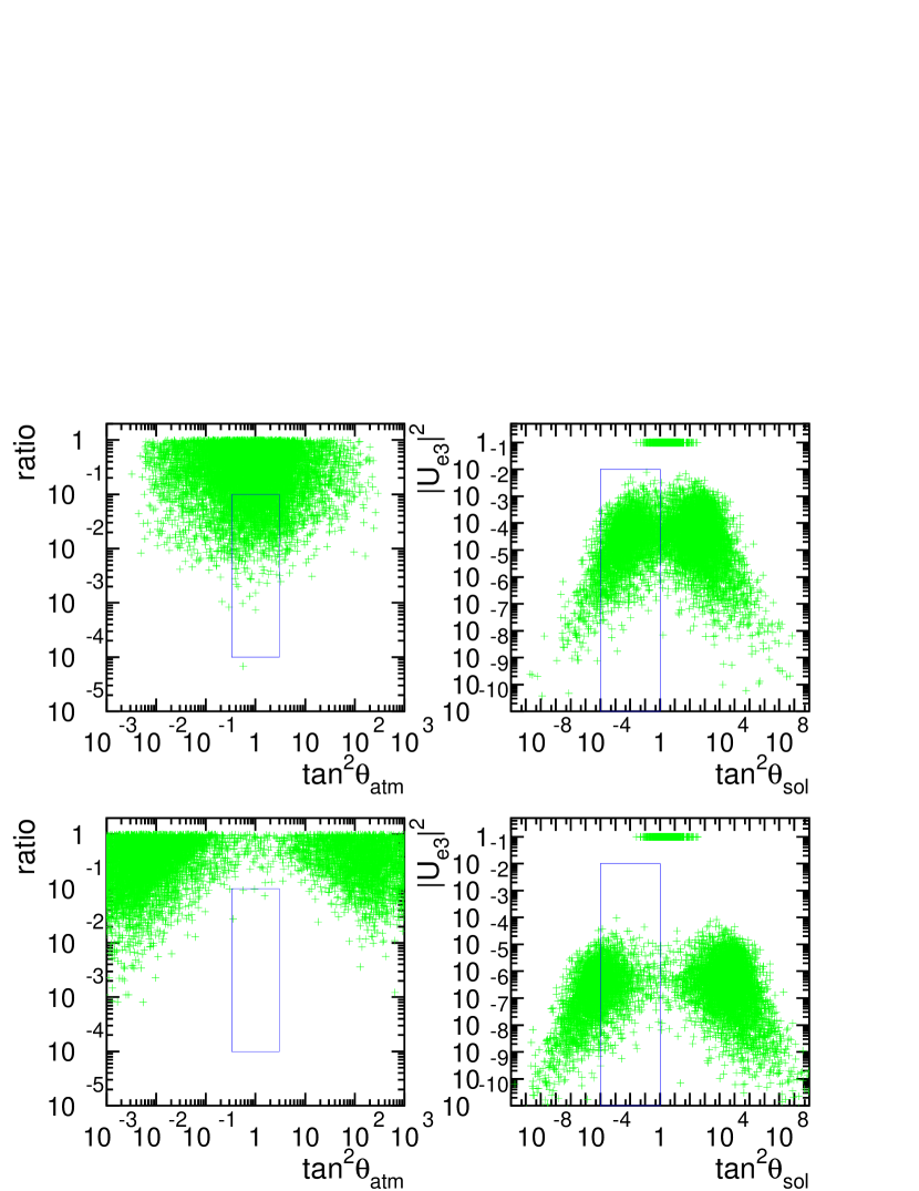
Figure 7: Neutrino mixing parameters obtained for 10001 randomly generated Majorana mass matrices, imposing constraints from the absence of flavour violating charged lepton decays (see text) displayed in the following manner: $ratio\equiv\Delta m^{2}_{\odot}/\Delta m^{2}_{\rm atm}\times\tan^{2}\theta_{\rm atm}(left)$ and $|U_{e3}|^{2}\times\tan^{2}\theta_{\odot}$ (right). In the top, the branching ratios for flavour changing lepton decays are close to the current experimental bounds [9], while the bottom figures explore the behaviour of the oscillation parameters as the prediction for the branching ratios for flavour changing charged lepton decays decreases (see text for details).

More significant than the figures, perhaps, are the following numerics: 51% of the points yield $1/3<\tan^{2}\theta_{\rm atm}<3$, while 22% (1.5%) of the points yield $ratio<10^{-1}$ ($10^{-2}$), and 38% of the points yield $10^{-5}<\tan^{2}_{\odot}<1$ (note that the values of $ratio$ we obtain are not small enough to accommodate the LOW of VAC solutions to the solar neutrino puzzle). Combining all constraints, 1.5% satisfy $1/3<\tan^{2}\theta_{\rm atm}<3$, $10^{-1}<ratio<10^{-3}$, $0.1<\tan^{2}_{\odot}<1$, $|U_{e3}|^{2}<0.1$ (LMA-like solution) and 0.1% satisfy $1/3<\tan^{2}\theta_{\rm atm}<3$, $10^{-2}<ratio<10^{-4}$, $10^{-5}<\tan^{2}_{\odot}<2\times 10^{-3}$, $|U_{e3}|^{2}<0.1$ (SMA-like solution).

What do these numbers imply? While most points do not yield phenomenologically acceptable parameters, there is a slightly more than 1% chance for obtaining the LMA solution with completely random order one Yukawa couplings. We do not consider this too “unlikely,” but leave definitive conclusions to the reader. One concrete statement, however, is that obtaining the SMA solution under these conditions is certainly less likely (15 times). The reason for this is that the SMA solution requires a larger hierarchy for the mass-squared differences, which is very hard to obtain with order one random Yukawa couplings.

What happens as the separation between left-handed lepton fields increases? Fig. 7(bottom, left) depicts the obtained values of $ratio\times\tan^{2}\theta_{\rm atm}$ if the same procedure is repeated, except that the suppression factor for the $\mu\tau$-element is increased by a factor of 10 (from 0.5 to 0.05). The results are rather striking. Unlike the previous case, depicted in Fig 7(top, left), large atmospheric mixing becomes more “rare” (11% of the points yield $1/3<\tan^{2}\theta_{\rm atm}<3$), especially when $ratio$ is required to be small (0.04% percent (none) of the cases satisfy $1/3<\tan^{2}\theta_{\rm atm}<3$ and $ratio<0.1$ (0.01)!). Therefore, in light of the observed hierarchy of neutrino mass-squared differences, large mixing in the atmospheric sector becomes exceedingly unlikely as the separation between $l_{\mu}$ and $l_{\tau}$ increases.

On the other hand, Fig. 7(bottom, right) depicts the obtained values of $|U_{e3}|^{2}\times\tan^{2}\theta_{\odot}$ when the original procedure is again performed, but restraining $\epsilon<0.01$. When compared to Fig. 7(top, right), it is easy to see that large mixing in the solar sector happens for a smaller fraction of all randomly generated matrices. The number of potentially good candidates is still reasonable: 28% of all matrices yield $10^{-5}<\tan^{2}_{\odot}<1$. Here, however, the probability of obtaining LMA-like solutions (see discussion related to Fig. 7(top)) decreases (0.3% compared to 1.5%), while the number of SMA-like solutions remains the same. Of course, this behaviour is expected, and the situation deteriorates very rapidly as the upper bound on $\epsilon$ decreases.

In summary, if neutrinos have a naturally small Majorana mass matrix, the AS solution to flavour changing charged lepton decays and the hierarchy of charged lepton masses naturally predicts that the neutrino masses are not strongly hierarchical and that mixing angles are rather small. In order to obtain large enough atmospheric mixing angles, we were forced to live very close to the current experimental bounds imposed by the searches for charged lepton flavour violation. We dare not make any precise predictions given the qualitative nature of our estimates, but if flavour violating $\mu$ and (especially) $\tau$ decays are not observed by the next generation of experiments [21], the scenario discussed in this section will be severely constrained, if not entirely ruled out.

This is to be contrasted to the study in the previous section, where neutrino mixing angles were also generically predicted to be small, while the masses were hierarchical. In order to obtain large mixing angles, we were forced to impose specific positions for the different leptonic fields. All solutions we found were either immediately ruled out by searches for lepton flavour violating processes, or predicted that their branching ratios were severely suppressed, out of reach of any foreseeable experiment. The price paid for these solutions was having to finely tune a priori unrelated distances to more than 1 part in $10^{2}$.

5 Summary and Conclusions

We have analysed the issue of charged lepton flavour violation and neutrino masses in the fat-brane paradigm proposed by Arkani-Hamed and Schmaltz (AS scenario). The AS scenario is particularly suited for explaining the absence of lepton flavour violating muon and tau decays, and can also naturally explain why neutrinos are more than ten orders of magnitude lighter than the top quark, if right-handed neutrinos are introduced in the brane.

We found that, indeed, the branching ratios for flavour violating muon and tau decays can be very easily suppressed to levels below the current experimental bounds, and that very small neutrino masses can be obtained for separations of order $10\mu^{-1}$. The AS scenario, however, seems to have a harder time accounting for the large neutrino mixing which has been observed in the atmospheric neutrino data. This is a peculiar feature of the AS scenario for fermion masses: it naturally accommodates large mass hierarchies and small mixing angles, while it seems to require additional “structure” (e.g., different pairs of fields have to be separated by very similar distances) in order to explain large mixing angles.

We studied the case of two lepton families in detail. The situation seems “finely tuned” when the the bounds imposed by charged lepton flavour violation are also taken into account. We showed that the charged lepton mass matrix is constrained to be quasi-diagonal, and that, in order to obtain large atmospheric mixing and the appropriate $\Delta m^{2}$, distances which are a priori unrelated are required to agree with one another better than one part in 100. We proceeded to analyse the case of three lepton flavours, and while we found that all the different solutions to the solar neutrino puzzle can be accommodated while keeping the absolute value of the $U_{e3}$ element of the leptonic mixing matrix small, we argued that the amount of fine-tuning required to simultaneously satisfy all neutrino data is “larger” than in the two-family case.

We then proceeded to discuss the effect of explaining the absence of flavour changing tau and muon decays and charged lepton masses in the AS scenario on theories where small Majorana neutrino masses are generated by breaking lepton number in a far away brane. In this case, in order to obtain large mixing in the atmospheric sector, we were forced to “approximate” different lepton doublet fields to the point that the current experimental upper bounds on the branching ratios of some rare tau and muon decays were almost saturated. Therefore, we expect these rare decays to be observed in the next round of experiments, if such a scenario were indeed realised in nature. Furthermore, very hierarchical neutrino mass-squared differences were not attainable, meaning that the solar neutrino puzzle would have to be solved either by the SMA or the LMA solutions.

In conclusion, we would like to emphasise that, in spite of the fine-tuning problems we highlighted in Sec. 3, the AS scenario should be regarded as a novel mechanism for understanding small mixing angles, which does not necessarily require the existence of fat branes or even large extra dimensions. Similar results are obtained in models with many different “thin” branes which are separated in the extra dimensions. Furthermore, if the extra dimensions are not large (and the hierarchy problem is solved by some other means), our results for neutrino masses and mixing angles would still apply, except for the flavour changing constraints from charged lepton decays, which would be absent. Finally, the fine-tuning which we pointed out could (and should, in our opinion) be interpreted as a challenge to be faced by candidates for the localising mechanism and/or the structure of the compact dimensions.

Appendix A Numerical Scan of the 3 Generation Parameter Space

In this appendix, we describe a numerical scan over the three generation, one extra dimension location space of the lepton doublets and right-handed neutrino singlets. In this case, specifying five distances suffices to determine the relative distance between the six different fermion fields. These distances are pictorially defined in Fig. 8, and are: $l_{1}$, $l_{2}$, $l_{3}$, the distances between $l_{\alpha}$ and $n_{\alpha}$, $\alpha=e,\mu,\tau$; $x$, the distance between $n_{\tau}$ and $n_{e}$; $y$, the distance between $n_{\tau}$ and $n_{\mu}$. Note that the sign of four out of the five distances is also meaningful (for example, when $y<0$, $n_{\mu}$ is “to the right” of $n_{\tau}$).

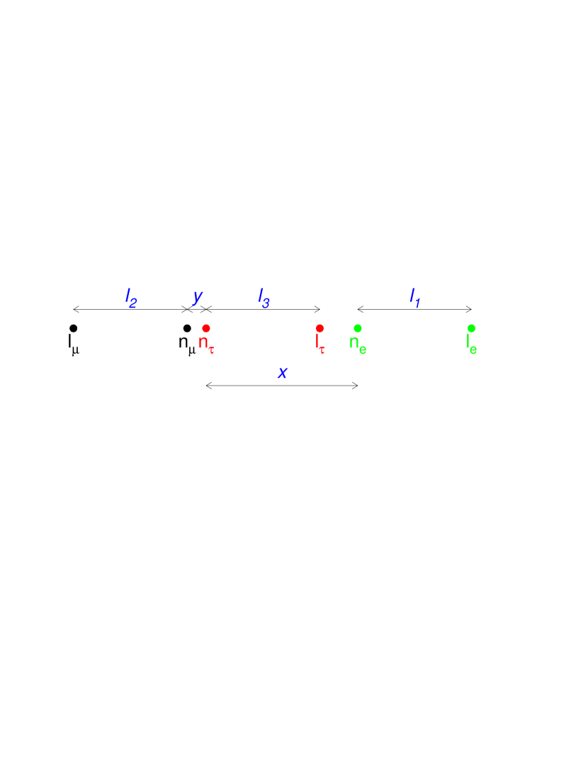
Figure 8: General three family configuration in one extra dimension. There are five independent distances, which are chosen to be $l_{1},l_{2},l_{3},x,y$. Note that in order to span the entire location space, four out of the five parameters should take positive and negative values, while the sign of the fifth one remains fixed.

In the scan, we varied $l_{1}$ ($l_{2}$) from $-20\mu^{-1}$ to $20\mu^{-1}$ ($-20.1\mu^{-1}$ to $20.1\mu^{-1}$ ) in steps of 0.2, $x$ and $y$ from $-20\mu^{-1}$ to $20\mu^{-1}$ in steps of 0.4, and $l_{3}$ from $0.1\mu^{-1}$ to $20.1\mu^{-1}$ in steps of 0.2. Out of all the points, we only consider these which yield neutrino mass matrices such that $(m_{\nu}m_{\nu}^{\dagger})_{ij}<10$ eV² for all $i,j=e,\mu,\tau$. This is done in order to guarantee that all neutrino masses squared are roughly less than 10 eV². One consequence of this constraint is that for all $l_{i}$, $|l_{i}|\mathrel{\mathchoice{\lower 3.0pt\vbox{\halign{$\m@th\displaystyle\hfill#\hfil$\cr>\crcr\sim\crcr}}}{\lower 3.0pt\vbox{\halign{$\m@th\textstyle\hfill#\hfil$\cr>\crcr\sim\crcr}}}{\lower 3.0pt\vbox{\halign{$\m@th\scriptstyle\hfill#\hfil$\cr>\crcr\sim\crcr}}}{\lower 3.0pt\vbox{\halign{$\m@th\scriptscriptstyle\hfill#\hfil$\cr>\crcr\sim\crcr}}}}7.0$, while certain bands for $x$ and $y$ are excluded.

Of the remaining matrices, we identify the ones whose eigenvalues and eigenvectors fall in the following window:

$$|U_{e3}|^{2}<0.1,$$

$$1/3<(|U_{\mu 3}|/|U_{\tau 3}|)^{2}\equiv\tan^{2}\theta_{\rm atm}<3,$$

$$10^{-5}<(|U_{e2}|/|U_{e1}|)^{2}\equiv\tan^{2}\theta_{\odot}<10,$$

$$10^{-3}~{}{\rm eV^{2}}<(m_{3}^{2}-m_{2}^{2})\equiv\Delta m^{2}_{\rm atm}<10^{-2}~{}{\rm eV^{2}},$$

$$10^{-10}~{}{\rm eV^{2}}<(m_{2}^{2}-m_{1}^{2})\equiv\Delta m^{2}_{\odot}<10^{-4}~{}{\rm eV^{2}},$$ (A.1)

where we define the neutrino mixing matrix as $\nu_{i}=U_{\alpha i}\nu_{\alpha}$, where $\nu_{\alpha}$, $\alpha=e,\mu,\tau$ are weak eigenstates and $\nu_{i}$, $i=1,2,3$ are mass eigenstates, with masses $m_{i}$. The eigenstates are organised in ascending order of mass-squared. When $m_{3}^{2}-m_{2}^{2}>m_{2}^{2}-m_{1}^{2}$ (normal hierarchy), the window defined above contains the region of the parameter space which satisfies all of the experimental constraints [6]. If $m_{3}^{2}-m_{2}^{2}<m_{2}^{2}-m_{1}^{2}$ (inverted hierarchy) the same window can be used after relabelling the mass eigenstates $1\rightarrow 3\rightarrow 2\rightarrow 1$, and defining $(m_{2}^{2}-m_{3}^{2})\equiv\Delta m^{2}_{\rm atm}$. It should be noted that during the numerical scan we did not find any matrix which yields an inverted mass hierarchy and is consistent with the constraints imposed above.

The results of the scan are best described in words. Out of roughly $2\times 10^{9}$ initially selected matrices, only 440 fall within the window defined above. The events are rejected at the following rate: 99% fail the mass constraints. From the surviving points, 96% fail to satisfy the $\tan^{2}\theta_{\odot}$ constraint. From the remaining points, 97% fail the $\tan^{2}\theta_{\rm atm}$ constraint, while 98% of the remainder fall out of the $|U_{e3}|^{2}$ bound. Note that only one out of roughly 5 million events survives all the constraints we define above.

Many comments are in order. First, in should be readily noted that the two “angle constraints” combine to remove 99.9% of the candidate matrices, ten times more than the “mass constraints.” Second, it should be pointed out that the mass constraints and the angle constraints “commute”, in the sense that, independent of the order in which they are applied, the percentage of the points which is removed is the same. This implies that there is no correlation between the values of the masses and the values of the mixing angles. The same is not true for the $\tan^{2}\theta_{\odot}$ and $\tan^{2}\theta_{\rm atm}$ constraints. Third, the $|U_{e3}|^{2}$ constraint is highly correlated with the angle constraints. If applied first, the $|U_{e3}|^{2}$ constraint only cuts a small fraction of all the matrices, while if applied last, it removes a very significant fraction of the events which pass the angle constraints. Therefore, events which have a small $|U_{e3}|$ generically have very small mixing in the solar and/or the atmospheric sector. This can be understood from the qualitative discussion included in the beginning of Sec. 3: the AS scenario prefers small mixing angles, and a generic set of points will yield a mixing matrix which has only “0s” and “1s” (one 1 for each column and row). Therefore, if we impose $|U_{e3}|^{2}$ small, the generic matrices which are left have some other $U_{\alpha 3}$ and $U_{ei}$ which is close to one, which necessarily means that $\tan^{2}\theta_{\odot,\rm atm}$ are either very large or very small.

The selected points yield a varied spectrum of solar angles and masses-squared, and no value of $\Delta m^{2}_{\odot}$ and $\tan^{2}\theta_{\odot}$ is strongly preferred. All points, without exception, choose the second and third generation fields to fall into either the configuration depicted in Fig. 3(A) or Fig. 3(B) (note that the configurations where $n_{\mu}$ and $n_{\tau}$ are exchanged are, of course, also present in equal numbers), while $l_{1}$ and $n_{1}$ are placed in various locations. Furthermore, the choices for $l$ and $\delta$ in the case of the configuration Fig. 3(A), and $l_{21}$ and $l_{22}$ in the case of configuration Fig. 3(B) are exactly the ones obtained in the last line of Tables 1 and 2, respectively. This implies, as one would naively expect, that in order to obtain large mixing in the “atmospheric sector” the same tuning of parameters as the ones discussed in Sec. 3.1 is required.

Fig. 9(left) is a scatter plot of the values of $l_{2}$ and $l_{1}$ of the points which pass all of the constraints mentioned above. The light [green] points are the ones which also pass the constraints that two lepton doublets are not too close to one another (flavour changing constraints): $|l_{\tau}-l_{e,\mu}|\mathrel{\mathchoice{\lower 3.0pt\vbox{\halign{$\m@th\displaystyle\hfill#\hfil$\cr>\crcr\sim\crcr}}}{\lower 3.0pt\vbox{\halign{$\m@th\textstyle\hfill#\hfil$\cr>\crcr\sim\crcr}}}{\lower 3.0pt\vbox{\halign{$\m@th\scriptstyle\hfill#\hfil$\cr>\crcr\sim\crcr}}}{\lower 3.0pt\vbox{\halign{$\m@th\scriptscriptstyle\hfill#\hfil$\cr>\crcr\sim\crcr}}}}1\mu^{-1}$ and $|l_{\mu}-l_{e}|\mathrel{\mathchoice{\lower 3.0pt\vbox{\halign{$\m@th\displaystyle\hfill#\hfil$\cr>\crcr\sim\crcr}}}{\lower 3.0pt\vbox{\halign{$\m@th\textstyle\hfill#\hfil$\cr>\crcr\sim\crcr}}}{\lower 3.0pt\vbox{\halign{$\m@th\scriptstyle\hfill#\hfil$\cr>\crcr\sim\crcr}}}{\lower 3.0pt\vbox{\halign{$\m@th\scriptscriptstyle\hfill#\hfil$\cr>\crcr\sim\crcr}}}}3\mu^{-1}$ (see Fig. 1). This constraint is sufficient for satisfying all flavour changing constraints described in Sec. 2 and also guarantee that the mixing in the charged lepton sector is negligible. 218 out of the 440 points satisfy this extra requirement.

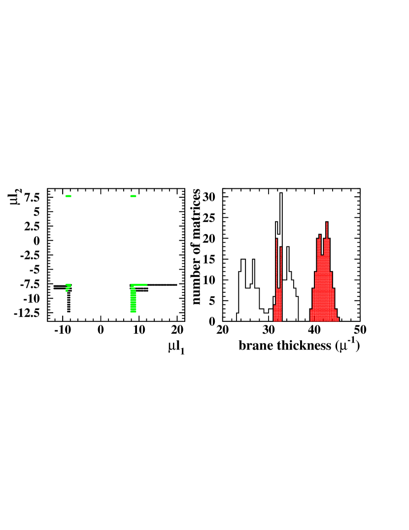
Figure 9: Scatter plot of $l_{2}\times l_{1}$ of all the 440 points which satisfy all constraints imposed by the neutrino data (left, see text). The light [green] points also satisfy the “flavour changing constraints,” $|l_{\tau}-l_{e,\mu}|>1\mu^{-1}$ and $|l_{\mu}-l_{e}|>3\mu^{-1}$. Histogram of the brane-thickness for the same 440 points (right). The painted histogram corresponds to events which satisfy the flavour changing constraints.

Fig. 9(right) is a histogram of the largest distance between two lepton fields, and can be interpreted as a lower bound on the brane “thickness.” The solid painted histogram is for points which satisfy the flavour changing constraints. Note that only “very thick” branes are obtained, especially for matrices which do not have two $l$s on top of each other. This could be the subject of serious concern, since branes should not be too “fat” if one wants to solve the gauge hierarchy problem and still have the gauge bosons propagate freely in the entire fat-brane (see [3] for details). We prefer, instead, to view this as an indication that one extra dimension seems to be problematic, and that if one considers branes which are fat in more dimensions similar configurations can be obtained for much “thiner” branes. This is very easy to see. All one has to do is rotate a number of lepton fields, keeping the “smaller” distances fixed, while making sure that the “larger” distances remain large. Because of the Gaussians dependency of the Yukawa couplings on the distances, these configurations will be, in practice, indistinguishable from the one-dimensional ones we discuss here.

One may worry whether configurations Fig. 3(C) and Fig. 3(D) can yield proper solar parameters, since these configurations never show up in our general scan. In order to check this, we numerically searched for solutions by starting from configurations Fig. 3(C) and Fig. 3(D), choosing distances such that the atmospheric neutrino puzzled is solved and varying the parameters $l_{1}$ and $x$ (see Fig. 8). Indeed, we are able to find a large number of solutions as long as $l_{\mu}$ is not on top of $l_{\tau}$, but extremely close. This is easy to understand: when $l_{\mu}$ is exactly on top of $l_{\tau}$, the neutrino mass matrix has a zero eigenvalue, whose eigenvector is very close to $1/\sqrt{2}(|\nu_{\mu}\rangle-|\nu_{\tau}\rangle)$. This implies that the $|\nu_{e}\rangle$ state is contained in the two heaviest mass eigenstates, which makes it very hard to solve the solar neutrino puzzle. The only alternative is to choose the other distances such that an inverted mass hierarchy is obtained, but such a situation is extremely finely-tuned. It should be noted that all solutions found starting from the configurations 3(C) and (D) are ruled out by flavour changing constraints. Indeed, as was pointed out in Sec. 3.1, the configuration Fig. 3(D) is already rule out in the case of two generations, while satisfactory solutions with the configuration Fig. 3(C) are extremely finely tuned.

Another worry is whether much thinner branes cannot be obtained. One possibility, for example, is to have all right-handed neutrinos very close to each other. Since we are restraining ourselves to only one dimension, these configurations are very hard to obtain, and the flavour changing constraints make them even harder to find. Nonetheless, we have been able to find (numerically) examples which fit this description and do not yield too large charged lepton mixing or flavour changing effects.

References

- [1] N. Arkani-Hamed, S. Dimopoulos, and G. Dvali, Phys. Lett. B429, 263 (1998); I. Antoniadis et al., Phys. Lett. B436, 257 (1998); N. Arkani-Hamed, S. Dimopoulos, and G. Dvali, Phys. Rev. D59, 086004 (1999).
- [2] N. Arkani-Hamed and M. Schmaltz, Phys. Rev. D61, 033005 (2000).
- [3] E. A. Mirabelli and M. Schmaltz, Phys. Rev. D61, 113011 (2000).
- [4] G.C. Branco, A. de Gouvêa, and M.N. Rebelo, Phys. Lett. B506, 115 (2001).
- [5] N. Arkani-Hamed, Y. Grossman, and M. Schmaltz, Phys. Rev. D61, 115004 (2000); T.G. Rizzo, Phys. Rev. D61, 055005 (2000); hep-ph/0101278.
- [6] For a complete compilation of the recent neutrino data, see the Proceedings of the XIX International Conference on Neutrino Physics and Astrophysics, Sudbury, Canada 16–21 June 2000, eds. J. Law, R.W. Ollerhead, and J.J. Simpsom, Nucl. Phys. B (Proc. Suppl.) 91 (2001); Super Kamiokande Coll. (S. Fukuda et al.), hep-ex/0103032; hep-ex/0103033. For recent combined analyses of the atmospheric and/or solar and/or reactor neutrino data in terms of neutrinos oscillations see J.N. Bahcall, P.I. Krastev, A.Yu. Smirnov, hep-ph/0103179; M.C. Gonzalez-Garcia, et al., Phys. Rev. D63, 033005 (2001); G.L. Fogli, E. Lisi, and A. Marrone, Phys. Rev. D63, 053008 (2001); M.C. Gonzalez-Garcia and C. Peña-Garay, Nucl. Phys. B (Proc. Suppl.) 91, 80 (2001); G.L. Fogli, et al Nucl. Phys. B (Proc. Suppl.) 91, 167 (2001); S. Goswami, D. Majumdar, and A. Raychaudhuri, Phys. Rev. D63, 013003 (2001). N. Fornengo, M.C. Gonzalez-Garcia, and J.W.F. Valle, Nucl. Phys. B580, 58 (2000); and many references therein.
- [7] Super-Kamiokande Collaboration (M. Shiozawa et al.) Phys. Rev. Lett. 81, 3319 (1998); Super-Kamiokande Collaboration (M. Hayato et al.) Phys. Rev. Lett. 83, 1529 (1999).
- [8] Y. Kuno and Y. Okada, hep-ph/9909265.
- [9] D. E. Groom et al. (Particle Data Group), Eur. Phys. J. C 15, 1 (2000).
- [10] N. Arkani-Hamed et al., hep-ph/9811448, K.R. Dienes, E. Dudas and T. Gherghetta, Nucl. Phys. B557, 25 (1999).
- [11] See, for example, A. Ioannisian, J.W.F. Valle, Phys. Rev. D63, 073002 (2001); D.O. Caldwell, R.N. Mohapatra, S.J. Yellin, hep-ph/0102279; hep-ph/0010353; A. Lukas et al., hep-ph/0011295; hep-ph/0008049; K. Agashe, G.-H. Wu, Phys. Lett. 498, 230 (2001). K.R. Dienes, I. Sarcevic, Phys. Lett. B500,133 (2001); E. Ma, G. Rajasekaran, U. Sarkar, Phys. Lett. B495, 363 (2000); R.N. Mohapatra, A. Pérez-Lorenzana Nucl. Phys. B593, 451 (2001); Nucl. Phys. B576 466 (2000); G.C. McLaughlin, J.N. Ng, Phys. Rev. D63, 053002 (2001); R. Barbieri, P. Creminelli, and A. Strumia, Nucl.Phys. B585, 28 (2000); A. Das, O.C.W. Kong, Phys. Lett. B470, 149 (1999); K. Yoshioka, Mod. Phys. Lett. A15, 29 (2000); G. Dvali and A.Yu. Smirnov, Nucl. Phys. B563, 63 (1999); A.E. Faraggi, M. Pospelov Phys. Lett. B458, 237 (1999).
- [12] S. Nussinov and R. Shrock, hep-ph/0101340.
- [13] L. Hall, H. Murayama, and N. Weiner, Phys. Rev. Lett. 84, 2572 (2000); N. Haba and H. Murayama, hep-ph/0009174.
- [14] A. de Gouvêa and J.W.F. Valle, Phys. Lett. B501, 115 (2001).
- [15] Talk by H. Sobel for the Super-Kamiokande Collaboration at the Neutrino 2000 conference (see [6]), Nucl. Phys. B (Proc. Suppl.) 91, 127 (2001).
- [16] CHOOZ Coll. (M. Apollonio et al.), Phys. Lett. B466, 415 (1999); Palo Verde Coll. (F. Boehm et al.), Nucl. Phys. (Proc. Suppl.) 77, 166 (1999).
- [17] LSND Coll. (C. Athanassopoulos et al.), Phys. Rev. Lett. 75, 2650 (1995); Phys. Rev. Lett. 77, 3082 (1996); Phys. Rev. Lett. 81 1774 (1998); talk by W.C. Louis for the LSND Collaboration at the Neutrino 2000 conference (see [6]), Nucl. Phys. B (Proc. Suppl.) 91, 198 (2001).
- [18] First reference in [10].
- [19] N. Arkani-Hamed and S. Dimopoulos, hep-ph/9811353.
- [20] H.V. Klapdor-Kleingrothaus et al., in Proceedings of the Third Internationl Conference on Dark Matter in Astro and Particle Physics, DARK2000, Heidelberg, Germany, 10–16 July 2000, Springer, Heidelberg (2001), ed. H.V. Klapdor-Kleingrothaus, hep-ph/0103082.
- [21] L. Barkov et al., “Search for down to branching ratio,” available at http://www.icepp.s.u-tokyo.ac.jp/meg; L. Serin and R. Stroynowski, ATL-PHYS-97-114 (1997), “Study of lepton number lepton number violating decay in ATLAS.”
- [22] A. de Gouvêa, A. Friedland, and H. Murayama, JHEP 0103, 009 (2001); Phys. Lett. B490, 125 (2000). See also the three neutrino analyses of the solar neutrino puzzle in [6].