IUHET 432

April 2001

CROSS SECTIONS AND LORENTZ VIOLATION Don Colladay^a and V. Alan Kostelecký^b

^aNew College, University of South Florida,
Sarasota, FL 34243, U.S.A.

^bPhysics Department, Indiana University
Bloomington, IN 47405, U.S.A.

The derivation of cross sections and decay rates in the Lorentz-violating standard-model extension is discussed. General features of the physics are described, and some conceptual and calculational issues are addressed. As an illustrative example, the cross section for the specific process of electron-positron pair annihilation into two photons is obtained.

1. Introduction. The possibility of small violations of Lorentz invariance in quantum field theory is theoretically and experimentally viable [2]. At the level of the standard model, a general Lorentz-violating standard-model extension is known [3]. Its lagrangian consists of all possible terms involving standard-model fields that are observer Lorentz scalars, including terms having coupling coefficients with Lorentz indices. Gauge invariance is usually imposed. At low energies, the relevant operators are renormalizable and are all given in Ref. [3]. The domain of validity of the renormalizable terms in the fermion sector is known to be below the Planck scale or, for some operators, below the geometric mean of the low-energy scale and the Planck scale [4]. Above this scale, the nonrenormalizable terms would play a crucial role in maintaining causality and stability of the theory.

Various experiments have placed bounds on parameters in the standard-model extension, including comparative tests of quantum electrodynamics (QED) in Penning traps [5, 6, 7, 8], spectroscopy of hydrogen and antihydrogen [9, 10], measurements of muon properties [11, 12], clock-comparison experiments [13, 14, 15, 16], observations of the behavior of a spin-polarized torsion pendulum [17, 18], measurements of cosmological birefringence [19, 3, 20, 21], studies of neutral-meson oscillations [22, 23, 24], and observations of the baryon asymmetry [25]. However, relatively little is known about the implications of the theory for scattering experiments or particle decays. For instance, although a consistent quantization and the associated Feynman rules are known, no complete calculation of a scattering process in the context of the standard-model extension has been performed to date.

In the present work, we describe a general procedure for the calculation of cross sections and decay rates in the standard-model extension. Some of the usual concepts and tools are based on Lorentz invariance, so alternative procedures are needed. As an illustrative example, we obtain the cross section for the specific process of relativistic electron-positron pair annihilation into two photons, using the general Lorentz-violating extension of QED. The presence of Lorentz violation introduces new physical features, as shown below. For example, the violation of rotational invariance implies that the scattering cross section depends on the orientation of the colliding beams, which in turn produces in physical observables a sidereal-time dependence arising from the Earth’s rotation.

2. General considerations. We begin with some general issues affecting the calculation of cross sections and decay rates in the standard-model extension. For simplicity in what follows, specific examples are restricted to the theory of electrons, positrons, and photons in the presence of Lorentz and CPT violation. This QED extension is a limit of the full standard-model extension, and the methods used below apply directly to the complete theory.

It is useful first to recap the definition and some properties of the general Lorentz- and CPT-violating QED extension. Its lagrangian is [3]

$${\cal L}={\textstyle{1\over 2}}i\overline{\psi}\Gamma^{\nu}\stackrel{{\scriptstyle\leftrightarrow}}{{D_{\nu}}}\psi-\overline{\psi}M\psi-{\textstyle{{1}\over{4}}}F_{\mu\nu}F^{\mu\nu}+{\textstyle{1\over 2}}{(k_{AF})}^{\kappa}\epsilon_{\kappa\lambda\mu\nu}A^{\lambda}F^{\mu\nu}-{\textstyle{{1}\over{4}}}{(k_{F})}_{\kappa\lambda\mu\nu}F^{\kappa\lambda}F^{\mu\nu}.$$ (1)

In this equation,

$${\Gamma}^{\nu}={\gamma}^{\nu}+c^{\mu\nu}{\gamma}_{\mu}+d^{\mu\nu}{\gamma}_{5}{\gamma}_{\mu}+e^{\nu}+if^{\nu}{\gamma}_{5}+{\textstyle{{1}\over{2}}}g^{\lambda\mu\nu}{\sigma}_{\lambda\mu},$$ (2)

and

$$M=m+a_{\mu}{\gamma}^{\mu}+b_{\mu}{\gamma}_{5}{\gamma}^{\mu}+{\textstyle{{1}\over{2}}}H^{\mu\nu}{\sigma}_{\mu\nu}.$$ (3)

Here, $m$ is the electron mass, while the quantities $a_{\mu}$, $b_{\mu}$, $c_{\mu\nu}$, $d_{\mu\nu}$, $e_{\mu}$, $f_{\mu}$, $g_{\lambda\mu\nu}$, $H_{\mu\nu}$, ${(k_{AF})}_{\kappa}$, ${(k_{F})}_{\kappa\lambda\mu\nu}$ are real coefficients controlling the Lorentz violation.

The Lorentz-violating terms in the lagrangian (1) produce effects both in relativistic quantum mechanics and in quantum field theory [3, 4]. In quantum theory, the presence of extra time derivatives in the quadratic fermion component of Eq. (1) implies that the time evolution of $\psi$ is unconventional, so the asymptotic states associated with $\psi$ cannot be directly identified with physical free-particle states. To avoid these interpretational difficulties, the extra time-derivative factors can be eliminated via a spinor redefinition [5]

$$\psi=A\chi,$$ (4)

where $A$ is an invertible matrix satisfying $A^{\dagger}\gamma^{0}\Gamma^{0}A=1$. This redefinition leaves the physics unchanged but yields the conventional Schrödinger time evolution for $\chi$, $i\partial_{0}\chi=H\chi$. The quanta created by $\chi$ can therefore be identified with physical particles. The modified hamiltonian $H$ is hermitian and is given by

$$H=\gamma^{0}\overline{A}(-i\Gamma_{j}D^{j}+M)A,$$ (5)

where $\overline{A}\equiv\gamma^{0}A^{\dagger}\gamma^{0}$. Details about the existence of the spinor redefinition and the properties of the matrix $A$ can be found in Ref. [4].

Since $A$ is chosen by definition to eliminate time derivatives, its form depends on the specification of the time coordinate and hence on the choice of observer inertial frame. This induces a noncovariant relationship between $\chi$ in the chosen frame and the corresponding physical spinor in another frame boosted relative to the first. Awareness of this feature of the spinor redefinition is crucial in calculating scattering cross sections or decay rates, since several of the standard procedures rely upon conversions between various special frames such as the rest frame, the center-of-momentum frame, or the laboratory frame. Transformations between inertial frames can still be implemented, but the additional complexity arising from the associated transformations of $A$ makes it easier in practice to adopt calculational methods that avoid frame changes. We emphasize that all these complications are purely technical, since the physics is guaranteed to be independent of the choice of observer inertial frame by virtue of observer Lorentz invariance [3].

The calculation of cross sections or decay rates parallels the conventional approach with some modifications. The $S$-matrix element and the corresponding transition probability per unit time and volume can be calculated from Feynman diagrams in the standard way, but with appropriately modified Feynman rules [3]. Associated to the lagrangian (1) is a conserved canonical energy-momentum tensor, and the corresponding energy-momentum 4-vector $p^{\mu}$ is conserved at the vertices of the Feynman diagrams as usual. This generates the standard overall momentum $\delta$-function factor. For external legs on a diagram, spinor solutions of the modified Dirac equation must be derived and used. Internal lines in Feynman graphs are associated with a modified propagator, which in the case of fermions in the QED extension takes the form

$$S_{F}(p)={{1}\over{\gamma^{0}E-\overline{A}\vec{\Gamma}A\cdot\vec{p}-\overline{A}MA}}.$$ (6)

This propagator for $\chi$ is appropriate for calculations of physical observables in scattering processes. Note that it differs from the propagator for $\psi$, which has been used to study microcausality of the theory [4].

As usual, to obtain the cross section or decay rate, the transition probability per unit time and volume must be divided by a factor $F$ accounting for properties of the initial state. For example, for the scattering between two beams of particles, this factor is normally defined as the product of the beam densities $N_{1}$, $N_{2}$ and the modulus of the beam velocity difference $|\vec{v}_{1}-\vec{v}_{2}|$:

$$F=N_{1}N_{2}|\vec{v}_{1}-\vec{v}_{2}|.$$ (7)

In the conventional case, Lorentz invariance and the momentum-velocity relation $\vec{p}=E\vec{v}$ are then often exploited to write $F$ in the covariant form $4[(p_{1}\cdot p_{2})^{2}-m^{4}]^{1/2}$, with the field normalizations chosen so that the densities are $N_{1}=2E_{1}$, $N_{2}=2E_{2}$.

In the present Lorentz-violating case, Eq. (7) still holds by definition but some care is required in its application because the momentum-velocity relation is modified and because the frame-dependence of the field redefinition (4) complicates the transformation of $F$ between frames. It is therefore most convenient to calculate the entire cross section in a single inertial frame. In the chosen frame, the factor $F$ is obtained from Eq. (7). The beam densities are derived using the time component of the conserved current, as usual. The beam velocities are calculated from the dispersion relation, via the definition of the group velocity of a wave packet with momentum $\vec{p}$:

$$\vec{v}_{g}\equiv\vec{\nabla}_{p}E(\vec{p}).$$ (8)

The reader is reminded that the group velocity $\vec{v}_{g}$ and the phase velocity $\vec{v}_{p}\equiv E\hat{p}/|\vec{p}|$ typically differ in orientation in the Lorentz-violating case [3]. Finally, the result for $F$ can be combined with the transition probability per unit time and volume to yield the physical cross section for any given process in the presence of Lorentz violation.

3. Relativistic electrons and positrons. A standard class of experiments in QED involves relativistic electron-positron collisions. In this case, the treatment of the fermion sector of the lagrangian (1) simplifies, as is discussed next.

In the relativistic limit, effects from the nonderivative couplings in Eq. (1) associated with the coefficients $a_{\mu}$, $b_{\mu}$, $H_{\mu\nu}$ are suppressed relative to other Lorentz-violating terms. This suppression occurs because the effects of the derivative couplings on the dispersion relation grow with momentum, while those of the nonderivative couplings are momentum independent. We emphasize that even at high energies the effects of the derivative couplings remain small relative to the conventional behavior from the fermion kinetic term, since this also grows with momentum. The point is rather that effects from Lorentz-violating derivative couplings dominate those from nonderivative ones, so at relativistic momenta it is reasonable to neglect the effects of the coefficients $a_{\mu}$, $b_{\mu}$, $H_{\mu\nu}$. Note, however, that caution is necessary in considering effects above the ultrarelativistic scale determined by the geometric mean $\sqrt{mM_{P}}$ of $m$ and the Planck mass $M_{P}$, since above this scale nonrenormalizable corrections to the lagrangian (1) become essential to maintain causality and stability in the quantum theory [4]. Other effects may also arise at the string scale [26]. In the present work, we limit attention to the relativistic regime lying well above $m$ but below $\sqrt{mM_{P}}$.

To simplify further the analysis here, we disregard possible effects from the CPT-violating coefficients $e_{\mu}$, $f_{\mu}$, $g_{\lambda\mu\nu}$. These are zero in the exact QED limit of the standard-model extension because they are incompatible with the full SU(2)$\times$U(1) gauge symmetry, but in practice they might be induced through various radiative corrections [3]. Also, in most applications, the colliding electrons and positrons are unpolarized. For unpolarized beams, effects from $d_{\mu\nu}$ average to zero because the corresponding field term contains a $\gamma_{5}$ coupling, which induces a correction of opposite sign for $\chi_{L}$ and $\chi_{R}$.

The only remaining coefficient is $c_{\mu\nu}$, and the corresponding field operator produces the dominant Lorentz-violating effects in relativistic collisions of unpolarized electrons and positrons. The effective lagrangian for the fermions is therefore a subset of the QED extension (1):

$${\cal L}={\textstyle{1\over 2}}i(\eta_{\mu\nu}+c_{\mu\nu})\overline{\psi}\gamma^{\mu}(\stackrel{{\scriptstyle\leftrightarrow}}{{\partial^{\nu}}}+2iqA^{\nu})\psi-m\overline{\psi}\psi.$$ (9)

Without loss of generality, $c_{\mu\nu}$ can be taken traceless. To leading order in $c_{\mu\nu}$, the field redefinition (4) is explicitly found to be

$$\psi\equiv A\chi=(1-{\textstyle{1\over 2}}c_{\mu 0}\gamma^{0}\gamma^{\mu})\chi.$$ (10)

The lagrangian in terms of $\chi$ becomes

$${\cal L}={\textstyle{1\over 2}}i\tilde{\eta}_{{\mu\nu}}\overline{\chi}\gamma^{\mu}\stackrel{{\scriptstyle\leftrightarrow}}{{D^{\nu}}}\chi-\tilde{m}\overline{\chi}\chi,$$ (11)

where we have introduced the convenient notation

$$\tilde{m} \equiv m(1-c_{00}),$$

$$\tilde{\eta}_{{\mu\nu}} \equiv \eta_{{\mu\nu}}+{\cal C}_{{\mu\nu}},$$

$${\cal C}_{{\mu\nu}} \equiv c_{\mu\nu}-c_{\mu 0}\eta_{0\nu}+c_{\nu 0}\eta_{0\mu}-c_{00}\eta_{\mu\nu}.$$ (12)

These quantities have nontrivial Lorentz-transformation properties. For example, the effective electron mass $\tilde{m}$ depends on the observer inertial frame. Note that ${\cal C}_{\mu 0}=0$, which reflects the elimination of the time-derivative Lorentz-violating couplings in the lagrangian (11) for $\chi$. Note also that ${\cal C}_{\mu\nu}$ and hence $\tilde{\eta}_{\mu\nu}$ are typically not symmetric. However, ${\cal C}_{\mu\nu}$ may be symmetric under certain circumstances, such as in the special case of rotational invariance in the chosen inertial frame, where ${\cal C}_{\mu\nu}$ becomes a diagonal matrix with diagonal elements proportional to $(0,1,1,1)$.

To construct the relativistic quantum mechanics and the quantum field theory, we follow the general procedure described in Ref. [4]. The modified Dirac equation for the free $\chi$ fermion can be solved exactly using the plane-wave solution

$$\chi(x)=e^{-i\lambda_{\mu}x^{\mu}}w(\vec{\lambda}).$$ (13)

Using the leading-order results (10) and (12), the four-component spinor $w(\vec{\lambda})$ is found to satisfy

$$(\tilde{\eta}_{\mu\nu}\gamma^{\mu}\lambda^{\nu}-\tilde{m})w(\vec{\lambda})=0.$$ (14)

A nontrivial solution exists provided the determinant of the applied operator is zero. This leads to the dispersion relation

$$\tilde{\lambda}^{2}-\tilde{m}^{2}=0,$$ (15)

where we define $\tilde{\lambda}_{\mu}\equiv\tilde{\eta}_{\mu\nu}\lambda^{\nu}$. This dispersion relation holds to leading order in $c_{\mu\nu}$. It is quadratic in $\lambda^{0}(\vec{\lambda})$ and symmetric under $\lambda^{\mu}\rightarrow-\lambda^{\mu}$, implying that the roots are degenerate after reinterpretation. There are therefore no energy splittings between the fermion and antifermion solutions at this order, and the dispersion relation acquires only a momentum-dependent modification. We remark in passing that the exact dispersion relation for $\chi$ is identical to that for $\psi$ obtained from Eq. (9) and is given as Eq. (39) of Ref. [4], where some of its properties are also discussed. However, the form (15) suffices for our purposes and is convenient for calculation.

Define the positive root as $\lambda^{0}(\vec{p})=p^{0}(\vec{p})=E(\vec{p})$, where to leading order in $c_{\mu\nu}$ the energy $E$ is

$$E(\vec{p})=\sqrt{\vec{p}^{2}+\tilde{m}^{2}}-{{p^{j}{\cal C}_{jk}p^{k}}\over{\sqrt{\vec{p}^{2}+\tilde{m}^{2}}}}-{\cal C}^{0}_{\phantom{0}j}p^{j}.$$ (16)

The field $\chi(x)$ is expanded as

$$\chi(x)=\int{{d^{3}\vec{p}}\over{(2\pi)^{3}N(\vec{p})}}\sum_{\alpha=1}^{2}\left[b_{(\alpha)}(\vec{p})e^{-ip\cdot x}u^{(\alpha)}(\vec{p})+d_{(\alpha)}^{\dagger}(\vec{p})e^{ip\cdot x}v^{(\alpha)}(\vec{p})\right],$$ (17)

where the spinors are normalized to

$$u^{(\alpha)\dagger}(\vec{p})u^{(\alpha^{\prime})}(\vec{p})=\delta^{\alpha\alpha^{\prime}}N(\vec{p}) \quad v^{(\alpha)\dagger}(\vec{p})v^{(\alpha^{\prime})}(\vec{p})=\delta^{\alpha\alpha^{\prime}}N(\vec{p}),$$ ,

$$u^{(\alpha)\dagger}(\vec{p})v^{(\alpha^{\prime})}(-\vec{p})=0 \quad v^{(\alpha)\dagger}(-\vec{p})u^{(\alpha^{\prime})}(\vec{p})=0.$$ , (18)

We leave the normalization factor $N(\vec{p})$ arbitrary to display explicitly its cancellation in the physical cross section. The reader is cautioned that boosting the chosen value of $N(\vec{p})$ to another inertial frame is nontrivial because the spinor redefinition (10) must be taken into account.

Quantization is implemented by imposing the following nonvanishing anticommutation relations on the mode operators:

$$\{b_{(\alpha)}(\vec{p}),b^{\dagger}_{(\alpha^{\prime})}(\vec{p}^{~{}\prime})\} = (2\pi)^{3}N(\vec{p})\delta_{\alpha\alpha^{\prime}}\delta^{3}(\vec{p}-\vec{p}^{~{}\prime}),$$

$$\{d_{(\alpha)}(\vec{p}),d^{\dagger}_{(\alpha^{\prime})}(\vec{p}^{~{}\prime})\} = (2\pi)^{3}N(\vec{p})\delta_{\alpha\alpha^{\prime}}\delta^{3}(\vec{p}-\vec{p}^{~{}\prime}).$$ (19)

The resulting equal-time anticommutation relations for the $\chi$ field are conventional. The corresponding single-particle states are therefore normalized as usual according to $\langle p^{\prime},\alpha^{\prime}|p,\alpha\rangle=(2\pi)^{3}N(\vec{p})\delta_{\alpha\alpha^{\prime}}\delta^{3}(\vec{p}^{\prime}-\vec{p})$. Matching this normalization to that obtained from the representation (13) in relativistic quantum mechanics shows that the number density for an incident plane wave is normalized to $N(\vec{p})$ particles per unit volume.

The conserved canonical energy-momentum tensor is an observer Lorentz 2-tensor, which in terms of the redefined spinors $\chi$ in the chosen frame takes the form

$$\Theta^{{\mu\nu}}={{i}\over{2}}\tilde{\eta}_{\alpha}^{\ \mu}\overline{\chi}\gamma^{\alpha}\stackrel{{\scriptstyle\leftrightarrow}}{{\partial^{\nu}}}\chi.$$ (20)

The corresponding conserved four-momentum is diagonal in the creation and annihilation operators by virtue of the field redefinition:

$$P^{\mu} = \int d^{3}\vec{x}:\Theta^{0\mu}:$$ (21)

$$= \int{{d^{3}\vec{p}}\over{(2\pi)^{3}N(\vec{p})}}p^{\mu}\sum_{\alpha=1}^{2}\left[b_{(\alpha)}^{\dagger}(\vec{p})b_{(\alpha)}(\vec{p})+d_{(\alpha)}^{\dagger}(\vec{p})d_{(\alpha)}(\vec{p})\right].$$

The conserved U(1) current is an observer Lorentz 4-vector of the form

$$j^{\mu}=\tilde{\eta}_{\alpha}^{\phantom{\alpha}\mu}\overline{\chi}\gamma^{\alpha}\chi,$$ (22)

with conserved charge

$$Q=\int{{d^{3}\vec{p}}\over{(2\pi)^{3}N(\vec{p})}}\sum_{\alpha=1}^{2}\left[b_{(\alpha)}^{\dagger}(\vec{p})b_{(\alpha)}(\vec{p})-d_{(\alpha)}^{\dagger}(\vec{p})d_{(\alpha)}(\vec{p})\right].$$ (23)

To leading order in $c_{\mu\nu}$, the Feynman propagator (6) for $\chi$ can be written as

$$S_{F}(p)={{1}\over{\tilde{p}_{\mu}\gamma^{\mu}-\tilde{m}}}.$$ (24)

Equating the propagator to the vacuum expectation value of the usual time-ordered product of fields yields the useful identities

$$\sum_{\alpha=1}^{2}u^{(\alpha)}(\vec{p})\overline{u}^{(\alpha)}(\vec{p})={N(\vec{p})\over 2\tilde{E}(\vec{p})}({\not\hbox{\hskip-2.0pt}{\tilde{p}}}+\tilde{m}),\quad\sum_{\alpha=1}^{2}v^{(\alpha)}(\vec{p})\overline{v}^{(\alpha)}(\vec{p})={N(\vec{p})\over 2\tilde{E}(\vec{p})}({\not\hbox{\hskip-2.0pt}{\tilde{p}}}-\tilde{m}),$$ (25)

where $\tilde{E}(\vec{p})\equiv\tilde{p}_{0}(\vec{p})=\tilde{\eta}_{0\nu}p^{\nu}$ and the shorthand notation ${\not\hbox{\hskip-2.0pt}{\tilde{p}}}\equiv\tilde{\eta}_{\mu\nu}\gamma^{\mu}p^{\nu}$ is used. These relations are generalizations of the usual ones, and they can be verified by direct calculation using the explicit expressions for the modified spinors.

4. Cross section for $e^{-}e^{+}\to 2\gamma$. As an illustrative example of a cross-section calculation in the QED extension, we next apply the above general procedure to the pair annihilation of relativistic electrons and positrons into two photons. To simplify matters, we disregard Lorentz-violating effects in the photon sector associated with the coefficients ${(k_{AF})}_{\mu}$ and ${(k_{F})}_{\kappa\lambda\mu\nu}$. The former is in any case expected theoretically to be zero [3] and is bounded experimentally to less than about $10^{-42}$ GeV by astrophysical observations [19], while the latter is also known to be negligible on the relevant scale [3, 27].

The appropriate element of the transition matrix $T$ for the process $e^{-}e^{+}\rightarrow 2\gamma$ can be found by evaluating the tree-level diagrams for electron-positron annihilation, using the modified Feynman rules for the QED extension. The result is

$$iT_{fi} = -ie^{2}(2\pi)^{4}\delta^{4}(k_{1}+k_{2}-p_{1}-p_{2})\overline{v}(p_{2})\biggl{[}{\not\hbox{\hskip-2.0pt}{\tilde{\epsilon}_{2}}}{{1}\over{{\not\hbox{\hskip-2.0pt}{\tilde{p}_{1}}}-{\not\hbox{\hskip-2.0pt}{\tilde{k}_{1}}}-\tilde{m}}}{\not\hbox{\hskip-2.0pt}{\tilde{\epsilon}_{1}}}+(1\leftrightarrow 2)\biggr{]}u(p_{1})$$ (26)

$$\equiv i(2\pi)^{4}\delta^{4}(k_{1}+k_{2}-p_{1}-p_{2}){\cal T}_{fi}.$$

In this equation, $p_{1}$, $p_{2}$ are the electron and positron momenta, while $k_{1}$, $k_{2}$ are the photon momenta. The spinors $u$, $v$ solve the modified Dirac equation after the reinterpretation, while $\epsilon_{1}$, $\epsilon_{2}$ are the two photon polarization vectors. Note that crossing symmetry is satisfied, as expected.

Following the discussions above, it is most convenient to perform the whole calculation in a single inertial frame. Since in practice the experimental procedure involves detecting back-to-back photons in reconstructing the cross section, the appropriate frame is the center-of-momentum frame. This frame is also convenient for practical calculations.

The transition rate is determined by $\sum|{\cal T}_{fi}|^{2}$, where the sum is over final photon polarizations and initial fermion states. In accordance with the relativistic approximation, we treat $m$ as small and neglect subleading Lorentz-invariant factors of order $m^{2}/|\vec{p}|^{2}$. Taking advantage of the identities (25) and performing algebraic steps similar to those for the equivalent calculation in conventional QED yields in the center-of-momentum frame

$$\sum|{\cal T}_{fi}|^{2} = {4e^{4}N(\vec{p})N(-\vec{p})\over\tilde{E}(\vec{p})\tilde{E}(-\vec{p})}\biggl{\{}\biggl{(}{{1+\cos^{2}{\theta}}\over{\sin^{2}{\theta}}}\biggr{)}[1-2(c_{00}+c_{11}+c_{22}+c_{33})]$$ (27)

$$\qquad\qquad+{{4}\over{\sin^{4}{\theta}}}[\cos^{2}{\theta}\hat{p}c\hat{p}+\hat{k}c\hat{k}-\cos{\theta}(1+\cos^{2}{\theta})\hat{k}c\hat{p}]\biggr{\}},$$

which consists of the usual QED result plus order-$c_{\mu\nu}$ corrections. In this expression, $\hat{p}$ and $\hat{k}$ are unit vectors along the incident electron and outgoing photon directions, and $\cos\theta=\hat{p}\cdot\hat{k}$. Terms such as $\hat{k}c\hat{p}$ denote double contraction of the matrix $c_{jk}$ with the indicated unit vectors.

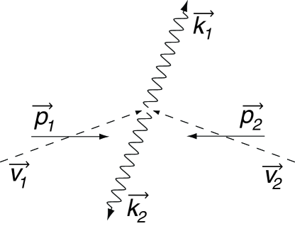
Figure 1: Momenta and velocities for the process $e^{-}e^{+}\to 2\gamma$. The incoming fermion momenta $\vec{p}_{1}$, $\vec{p}_{2}$ are equal and opposite, as are the outgoing photon momenta $\vec{k}_{1}$, $\vec{k}_{2}$ and velocities. The incoming fermion group velocities $\vec{v}_{1}$, $\vec{v}_{2}$, which determine the particle trajectories, typically are not parallel by virtue of the modified velocity-momentum relationship in Lorentz-violating quantum field theories.

The definition of the cross section also requires the calculation of the factor $F$ in Eq. (7). This must again be evaluated in the center-of-momentum frame. The frame dependence of the spinor redefinition (4) implies that it would, for example, be incorrect to proceed by calculating the flux and target density in the laboratory frame and applying standard transformation laws directly to boost the corresponding momenta back to the center-of-momentum frame. This would generate spurious factors of $\gamma^{2}$ that appear to dominate the cross section at high energies.

Keeping the normalizations arbitrary as before, it suffices to determine the beam velocity difference. Using Eqs. (8) and (15), the group velocity is found to be

$$v_{g}^{j}={1\over\tilde{E}}(\tilde{p}^{j}+{\cal C}_{\mu}^{\phantom{\mu}j}p^{\mu})$$ (28)

to lowest order in ${\cal C}_{\mu\nu}$. Note that this velocity typically does not lie along the momentum $\vec{p}$. Figure 1 illustrates the situation for the electron-positron pair annihilation. In the center-of-momentum frame, the momenta of the incoming beams are equal and opposite, but the velocities (which determine the trajectories) typically are not. For example, in the present case we find $v_{1}^{j}+v_{2}^{j}=2(c^{0j}+c^{j0})$, which can be nonzero.

Using Eq. (28), the velocity difference $|\vec{v}_{1}-\vec{v}_{2}|$ can be deduced. This in turn yields the factor $F$ in the center-of-momentum frame as

$$F=2N(\vec{p})N(-\vec{p})(1-\hat{p}{\cal C}\hat{p}).$$ (29)

In this equation and what follows, expressions such as $\hat{p}{\cal C}\hat{p}$ are understood to denote double contraction of the matrix ${\cal C}_{jk}$ with the indicated unit vectors. The reader is reminded that the beam velocity difference (which is about 2 rather than 1) is not the relative beam velocity obtained using a relativistic velocity-addition law. Note also that Lorentz-symmetric contributions of order $m^{2}/|\vec{p}|^{2}$ are neglected here but would be important in any considerations of microcausality [4].

Combining the results for the transition rate and the factor $F$ given in Eqs. (27) and (29), using conventional phase-space factors for the final-state photons, produces the cross section in the center-of-momentum frame:

$${d\sigma\over d\Omega} = {\alpha^{2}\over 4\vec{p}^{2}}\biggl{\{}\biggl{(}{1+\cos^{2}{\theta}\over\sin^{2}{\theta}}\biggr{)}(1+3\hat{p}{\cal C}\hat{p}+2{\cal C}_{\mu}^{\phantom{\mu}\mu})$$ (30)

$$\qquad\qquad+{{4}\over{\sin^{4}{\theta}}}[\cos^{2}{\theta}\hat{p}{\cal C}\hat{p}+\hat{k}{\cal C}\hat{k}-\cos{\theta}(1+\cos^{2}{\theta})\hat{k}{\cal C}\hat{p}]\biggr{\}}.$$

For definiteness, we choose coordinates with $\vec{p}_{1}$ along the 3 axis. Integrating this expression over the azimuthal angle $\phi$ then yields

$${{d\sigma}\over{d\cos\theta}} = \int_{0}^{2\pi}d\phi{{d\sigma}\over{d\Omega}}$$

$$= {{\pi\alpha^{2}}\over{2\vec{p}^{2}}}\left[\biggl{(}{{1+\cos^{2}{\theta}}\over{\sin^{2}{\theta}}}\biggr{)}(1+c_{00}+c_{33})-2\cot^{2}{\theta}(c_{11}+c_{22}-2c_{33})\right].$$

Note that the normalization factors have cancelled.

For other processes, fermions may be present in the final state. As usual, the available phase space $d\Pi$ per final state fermion is

$$d\Pi={{d^{3}\vec{p}}\over{(2\pi)^{3}N(\vec{p})}}.$$ (32)

In observable cross sections or decay rates, the normalization factors $N(\vec{p})$ again cancel with those in the transition probability. Note, however, that boosting $d\Pi$ to another inertial frame is typically nontrivial because the spinor redefinition (10) is involved.

5. Experimental signals. The cross section (30) is given in the center-of-momentum frame, and the components of the coefficients $c_{\mu\nu}$ for Lorentz violation are also defined in this frame. For symmetric colliders, the center-of-momentum frame coincides with the laboratory frame. However, the laboratory frame rotates with the Earth, so the spatial components of $c_{\mu\nu}$ oscillate periodically as functions of the sidereal time $t$. This induces corresponding variations in the observed cross section, with periodicities controlled by the Earth’s sidereal rotation frequency $\Omega\simeq 2\pi$/(23 h 56m).

To display explicitly the time dependence of the observable cross section, we introduce suitable bases of vectors for the nonrotating frame and the laboratory frame, following the notation and conventions of Ref. [14]. In this choice of coordinates, the right-handed basis $(\hat{X},\hat{Y},\hat{Z})$ for the nonrotating frame is compatible with celestial equatorial coordinates [28] with $\hat{Z}$ aligned along the rotation axis of the Earth. The other basis vectors lie in the plane of the equator, with $\hat{X}$ having declination and right ascension $0^{\circ}$, and $\hat{Y}$ having declination $0^{\circ}$ and right ascension $90^{\circ}$. Although this coordinate system is in fact only approximately fixed because the Earth precesses slowly over time, any induced effects are suppressed by several orders of magnitude and are neglected here.

We select the basis $(\hat{x},\hat{y},\hat{z})$ in the laboratory frame such that $\hat{z}\equiv\hat{p}_{1}$ is aligned along the direction of the electron-beam momentum. The vector $\hat{x}$ is fixed by requiring it to be perpendicular to $\hat{z}$ and to lie in the $\hat{z}$-$\hat{Z}$ plane. The remaining vector $\hat{y}$ is chosen to complete a right-handed triad: $\hat{y}=\hat{z}\times\hat{x}$. The angle between $\hat{z}$ and $\hat{Z}$ is denoted by $\chi$, so $\hat{z}\cdot\hat{Z}=\cos\chi$.

The transformation between the two sets of bases can be regarded as nonrelativistic to an excellent approximation. It is given by

$$\left(\begin{array}[]{c}\hat{x}\\ \hat{y}\\ \hat{z}\end{array}\right)=\left(\begin{array}[]{ccc}\cos{\chi}\cos{\Omega t}&\cos{\chi}\sin{\Omega t}&-\sin{\chi}\\ -\sin{\Omega t}&\cos{\Omega t}&0\\ \sin{\chi}\cos{\Omega t}&\sin{\chi}\sin{\Omega t}&\cos{\chi}\end{array}\right)\left(\begin{array}[]{c}\hat{X}\\ \hat{Y}\\ \hat{Z}\end{array}\right).$$ (33)

In what follows, we denote indices on the coefficients for Lorentz violation in the laboratory frame by $0,1,2,3$ and indices in the nonrotating frame by $0,X,Y,Z$.

To exhibit the sidereal-time dependence of the cross section, it suffices to apply the transformation (33) to the coefficients $c_{\mu\nu}$ for Lorentz violation. For example, the combinations of coefficients appearing in the cross section (LABEL:xsectth) become

$$\hbox{\hskip-20.0pt}c_{11}+c_{22}-2c_{33} = (c_{XX}+c_{YY}-2c_{ZZ})({\textstyle{{3}\over{2}}}\cos^{2}{\chi}-{\textstyle{1\over 2}})$$

$$-{\textstyle{{3}\over{2}}}(c_{XZ}+c_{ZX})\sin{2\chi}\cos{\Omega t}-{\textstyle{{3}\over{2}}}(c_{YZ}+c_{ZY})\sin{2\chi}\sin{\Omega t}$$

$$-{\textstyle{{3}\over{2}}}(c_{XX}-c_{YY})\sin^{2}{\chi}\cos{2\Omega t}-{\textstyle{{3}\over{2}}}(c_{XY}+c_{YX})\sin^{2}{\chi}\sin{2\Omega t},$$

$$c_{00}+c_{33} = c_{00}+c_{ZZ}+{\textstyle{1\over 2}}(c_{XX}+c_{YY}-2c_{ZZ})\sin^{2}{\chi}$$

$$+{\textstyle{1\over 2}}(c_{YZ}+c_{ZY})\sin{2\chi}\sin{\Omega t}+{\textstyle{1\over 2}}(c_{XZ}+c_{ZX})\sin{2\chi}\cos{\Omega t}$$

$$+{\textstyle{1\over 2}}(c_{XY}+c_{YX})\sin^{2}{\chi}\sin{2\Omega t}+{\textstyle{1\over 2}}(c_{XX}-c_{YY})\sin^{2}{\chi}\cos{2\Omega t}.$$

These endow the observable cross section with a dependence on sidereal time $t$ that has three components: a constant, an oscillation with period $T=2\pi/\Omega$, and an oscillation with period $T/2$.

Data in experiments are usually taken at different sidereal times and over several months. A typical analysis searching for deviations from QED in the cross section for $e^{-}e^{+}$ annihilation would therefore effectively average away the sidereal-time dependence. With coefficients expressed in the nonrotating coordinate system, the typical analysis is thus sensitive only to the average

$${{d\sigma}\over{d\cos\theta}}\biggr{|}_{\rm av} \equiv {{1}\over{T}}\int_{0}^{T}dt{{d\sigma}\over{d\cos\theta}}$$ (35)

$$= {{\pi\alpha^{2}}\over{2\vec{p}^{2}}}\biggl{\{}\biggl{(}{{1+\cos^{2}{\theta}}\over{\sin^{2}{\theta}}}\biggr{)}\Big{[}1+c_{00}+c_{ZZ}+{\textstyle{1\over 2}}(c_{XX}+c_{YY}-2c_{ZZ})\sin^{2}{\chi}\Big{]}$$

$$\qquad-2\cot^{2}{\theta}(c_{XX}+c_{YY}-2c_{ZZ})({\textstyle{{3}\over{2}}}\cos^{2}{\chi}-{\textstyle{{1}\over{2}}})\biggr{\}}.$$

This shows the time-averaged effect of the Lorentz-violating terms is the sum of a scaling of the usual cross section with a correction term proportional to $\cot^{2}{\theta}$.

The observation of sidereal variations in cross sections would provide a unique signal of Lorentz violation. In high-energy physics, analogous effects for neutral-meson oscillations have been used by the KTeV Collaboration to obtain a new constraint on coefficients for CPT violation in the standard-model extension [23]. Sidereal variations also form the basis for a variety of high-precision low-energy tests of the standard-model extension [8, 10, 12, 15, 16, 18]. However, to date constraints have been placed only on a few of the coefficients $c_{\mu\nu}$.

Large data sets of several hundred inverse picobarns for relativistic electron-positron pair annihilation have recently been collected by experiments at LEP [29]. These could in principle be used to bound the combinations of the coefficients $c_{\mu\nu}$ in the nonrotating frame that appear in Eqs. (LABEL:combs). Note that the Lorentz-violating modifications to the cross section (LABEL:xsectth) show no enhancement with energy, in accordance with the discussion at the beginning of section 3. This contrasts with corrections to the conventional QED cross section arising from other types of new physics, which typically grow with energy [30]. Although the necessary analysis and the systematics are qualitatively different in nature from those performed to date, it seems unlikely that sidereal-time binning of the $e^{-}e^{+}\to 2\gamma$ data would yield tight bounds. However, it could limit certain components of $c_{\mu\nu}$ otherwise presently unconstrained by experiment.

6. Summary. In this work, a procedure is presented for calculating observable cross sections and decay rates in the Lorentz-violating standard-model extension. In determining the transition matrix, conventional perturbative techniques apply but with modified Feynman rules. To avoid complexities associated with inertial-frame changes in the presence of Lorentz violation, it is most convenient to perform any analysis in a single frame. Methods for obtaining the necessary kinematical factors are also presented.

As an example, the process $e^{-}e^{+}\to 2\gamma$ for relativistic electrons and positrons is explicitly considered. In this case, the relevant coefficients for Lorentz violation are associated with derivative couplings in the fermion sector of the Lorentz-violating QED extension, and they scale with momentum like the usual fermion kinetic term. The contributions from other coefficients either are negligible or average to zero for unpolarized scattering. The resulting cross section is explicitly given in Eqs. (30) and (LABEL:xsectth). The Earth’s rotation induces a dependence of this cross section on sidereal time, specified in Eq. (LABEL:combs). High-statistics experiments searching for this effect could place bounds on some coefficients for Lorentz violation otherwise unconstrained by experiment.

It would be of interest to obtain expressions for other standard QED scattering amplitudes in the context of the Lorentz-violating QED extension. It is possible that the experimental sensitivity is enhanced by the boost factor $\gamma$ in appropriate circumstances. Certainly, sensitivity to different parameters can be expected among different processes. Also, the above arguments for neglecting certain coefficients for Lorentz violation fail for nonrelativistic fermions, so different scenarios such as fixed-target experiments could be worth investigation.

We thank Salvatore Mele for discussion. This work was supported in part by the United States Department of Energy under grant DE-FG02-91ER40661.

References

- [1]
- [2] For overviews of various theoretical ideas and experimental tests of Lorentz symmetry, see, for example, V.A. Kostelecký, ed., CPT and Lorentz Symmetry, World Scientific, Singapore, 1999.
- [3] D. Colladay and V.A. Kostelecký, Phys. Rev. D 55, 6760 (1997); Phys. Rev. D 58, 116002 (1998).
- [4] V.A. Kostelecký and R. Lehnert, Phys. Rev. D 63, 065008 (2001).
- [5] R. Bluhm et al., Phys. Rev. Lett. 79, 1432 (1997); Phys. Rev. D 57, 3932 (1998).
- [6] G. Gabrielse et al., in Ref. [2]; Phys. Rev. Lett. 82, 3198 (1999).
- [7] H. Dehmelt et al., Phys. Rev. Lett. 83, 4694 (1999).
- [8] R. Mittleman, I. Ioannou, and H. Dehmelt, in Ref. [2]; R. Mittleman et al., Phys. Rev. Lett. 83, 2116 (1999).
- [9] R. Bluhm et al., Phys. Rev. Lett. 82, 2254 (1999).
- [10] D.F. Phillips et al., Phys. Rev. D 63, 111101 (2001).
- [11] R. Bluhm et al., Phys. Rev. Lett. 84, 1098 (2000).
- [12] V.W. Hughes et al., presented at the Hydrogen II Conference, Tuscany, Italy, June, 2000.
- [13] V.W. Hughes, H.G. Robinson, and V. Beltran-Lopez, Phys. Rev. Lett. 4, 342 (1960); R.W.P. Drever, Philos. Mag. 6, 683 (1961); J.D. Prestage et al., Phys. Rev. Lett. 54, 2387 (1985); S.K. Lamoreaux et al., Phys. Rev. Lett. 57, 3125 (1986); Phys. Rev. A 39, 1082 (1989); T.E. Chupp et al., Phys. Rev. Lett. 63, 1541 (1989); C.J. Berglund et al., Phys. Rev. Lett. 75, 1879 (1995).
- [14] V.A. Kostelecký and C.D. Lane, Phys. Rev. D 60, 116010 (1999); J. Math. Phys. 40, 6245 (1999).
- [15] L.R. Hunter et al., in Ref. [2].
- [16] D. Bear et al., Phys. Rev. Lett. 85, 5038 (2000).
- [17] R. Bluhm and V.A. Kostelecký, Phys. Rev. Lett. 84, 1381 (2000).
- [18] B. Heckel et al., in B.N. Kursunoglu, S.L. Mintz, and A. Perlmutter, eds., Elementary Particles and Gravitation, Plenum, New York, 1999.
- [19] S.M. Carroll, G.B. Field, and R. Jackiw, Phys. Rev. D 41, 1231 (1990).
- [20] R. Jackiw and V.A. Kostelecký, Phys. Rev. Lett. 82, 3572 (1999).
- [21] M. Pérez-Victoria, Phys. Rev. Lett. 83, 2518 (1999); J.M. Chung, Phys. Lett. B 461, 138 (1999).
- [22] V.A. Kostelecký and R. Potting, Phys. Rev. D 51, 3923 (1995); D. Colladay and V.A. Kostelecký, Phys. Lett. B 344, 259 (1995); Phys. Rev. D 52, 6224 (1995); V.A. Kostelecký and R. Van Kooten, Phys. Rev. D 54, 5585 (1996); V.A. Kostelecký, Phys. Rev. Lett. 80, 1818 (1998); Phys. Rev. D 61, 016002 (2000); hep-ph/0104120; N. Isgur et al., in preparation.
- [23] KTeV Collaboration, Y.B. Hsiung et al., Nucl. Phys. Proc. Suppl. 86, 312 (2000).
- [24] OPAL Collaboration, R. Ackerstaff et al., Z. Phys. C 76, 401 (1997); DELPHI Collaboration, M. Feindt et al., preprint DELPHI 97-98 CONF 80 (July 1997); BELLE Collaboration, K. Abe et al., Phys. Rev. Lett. 86, 3228 (2001).
- [25] O. Bertolami et al., Phys. Lett. B 395, 178 (1997).
- [26] V.A. Kostelecký and S. Samuel, Phys. Rev. D 39, 683 (1989); ibid. 40, 1886 (1989); Phys. Rev. Lett. 63, 224 (1989); ibid. 66, 1811 (1991); V.A. Kostelecký and R. Potting, Nucl. Phys. B 359, 545 (1991); Phys. Lett. B 381, 89 (1996); Phys. Rev. D 63, 046007 (2001); V.A. Kostelecký, M. Perry, and R. Potting, Phys. Rev. Lett. 84, 4541 (2000).
- [27] V.A. Kostelecký and M. Mewes, in preparation.
- [28] R.M. Green, Spherical Astronomy, Cambridge University Press, Cambridge, 1985.
- [29] ALEPH Collaboration, R. Barate et al., Phys. Lett. B 429, 201 (1998); DELPHI Collaboration, P. Abreu et al., Phys. Lett. B 433, 429 (1998); Phys. Lett. B 491, 67 (2000); L3 Collaboration, M. Acciarri et al., Phys. Lett. B 413, 159 (1997); Phys. Lett. B 475, 198 (2000); OPAL Collaboration, K. Ackerstaff et al., Eur. Phys. J. C 1, 21 (1998); Phys. Lett. B 438, 379 (1998); Phys. Lett. B 465, 303 (1999).
- [30] O.J.P Éboli, A.A. Natale, and S.F. Novaes, Phys. Lett. B 271, 274 (1991).