LAPTH-842/01

NORDITA-2001-7 HE

SLAC-PUB-8818

hep-ph/0104291

STRUCTURE FUNCTIONS ARE NOT PARTON PROBABILITIES

Stanley J. Brodsky¹, Paul Hoyer^2,,

Nils Marchal^2,3, Stéphane Peigné³ and Francesco Sannino²

¹Stanford Linear Accelerator Center, Stanford CA 94309, USA

²Nordita, Blegdamsvej 17, DK–2100 Copenhagen, Denmark

³LAPTH, BP 110, F-74941 Annecy-le-Vieux Cedex, France

The common view that structure functions measured in deep inelastic lepton scattering are determined by the probability of finding quarks and gluons in the target is not correct in gauge theory. We show that gluon exchange between the fast, outgoing partons and target spectators, which is usually assumed to be an irrelevant gauge artifact, affects the leading twist structure functions in a profound way. This observation removes the apparent contradiction between the projectile (eikonal) and target (parton model) views of diffractive and small $x_{B}$ phenomena. The diffractive scattering of the fast outgoing quarks on spectators in the target causes shadowing in the DIS cross section. Thus the depletion of the nuclear structure functions is not intrinsic to the wave function of the nucleus, but is a coherent effect arising from the destructive interference of diffractive channels induced by final state interactions. This is consistent with the Glauber-Gribov interpretation of shadowing as a rescattering effect.

1. Introduction

Deep inelastic lepton scattering, $\ell N\to\ell^{\prime}+X$ (DIS) is central for our understanding of hadron structure. Ever since the earliest days of the parton model, it has been assumed that the leading-twist structure functions $F_{i}(x,Q^{2})$ measured in deep inelastic lepton scattering are determined by the probability to find quarks and gluons in the target [1]. This probability is given by the target wave function at the light-cone (LC) time when the current interacts (in the $q^{+}\leq 0$ frame). For example, the quark probability is distribution is

$${\cal P}_{{\rm q}/N}(x_{B},Q^{2})=\sum_{n}\int^{k_{i\perp}^{2}<Q^{2}}\left[\prod_{i}\,dx_{i}\,d^{2}k_{\perp i}\right]|\psi_{n}(x_{i},k_{\perp i})|^{2}\sum_{j=q}\delta(x_{B}-x_{j})$$ (1)

where the $\psi_{n}$ are LC wave functions of the target (see Eq. (2) below). The identification of structure functions with the square of light-front wave functions is usually made in the ghost-free LC gauge $n\cdot A=A^{+}=0$, the argument being that the path-ordered exponential in the operator product appearing in parton distributions (see Eq. (S0.Ex2) below) reduces to unity. Thus the DIS cross section appears to be fully determined by the probability distribution of partons in the target.

However, we shall show that this parton model interpretation of the structure functions, which was established for a theory with Yukawa couplings [1], is not correct in gauge theory. The critical issue is whether the scattering taking place after the virtual photon interacts can affect the leading twist cross section. It is well-known that in Feynman and other covariant gauges one has to include corrections to the “handbag” diagram due to final state interactions of the struck quark with the gauge field of the target. Light-cone gauge is singular – in particular, the gluon propagator $d_{LC}^{\mu\nu}(k)=\frac{i}{k^{2}+i\varepsilon}\left[-g^{\mu\nu}+\frac{n^{\mu}k^{\nu}+k^{\mu}n^{\nu}}{n\cdot k}\right]$ has a pole at $k^{+}=0$ which requires an analytic prescription. In final-state scattering involving on-shell intermediate states, the exchanged momentum $k^{+}$ is of ${\cal O}\left(1/\nu\right)$ in the target rest frame, which enhances the second term in the propagator. This enhancement allows rescattering to contribute at leading twist even in light-cone gauge.

We find that gluon exchange between the outgoing quarks and target spectators, which is usually assumed to be suppressed in the Bjorken limit, affects the leading twist structure functions in a profound way. Final state diffractive scattering gives rise to interference effects in the DIS cross section. Thus nuclear shadowing is not caused by the wave function of the nucleus, but is induced by final state interactions.

Thus the depletion of the nuclear structure functions is not intrinsic to the wave function of the nucleus, but in fact is a coherent effect reflecting the destructive interference of diffractive channels induced by the final state interactions.

The distinction between structure functions and parton probabilities is already implied by the Glauber-Gribov picture of nuclear shadowing [2, 3, 4, 5]. In this framework shadowing arises from interference between complex rescattering amplitudes involving on-shell intermediate states. In contrast, the wave function of a stable target is strictly real since it does not have on energy-shell configurations. A probabilistic interpretation of the DIS cross section is thus precluded.

Our paper thus explains the origins of nuclear shadowing and leading-twist diffraction, giving a new, first principle, perspective on these problems. Our formalism of final-state interactions has recently been used to analyze single-spin asymmetries in deep inelastic processes and to show that such asymmetries survive in the Bjorken limit, contrary to conventional arguments which claim that final state interactions are always power-law suppressed in the large scale of hard QCD processes [6].

2. The Foundations of the QCD-Improved Parton Model

Soon after the observation of Bjorken scaling (and before the advent of QCD) it was suggested [1] that the DIS cross section is fully determined by the target wave function. Specifically, consider the Fock expansion of the nucleon state $|{N}\rangle$ in terms of its quark and gluon constituents at equal Light-Cone (LC) time $\tau=t+z/c=y^{+}=y^{0}+y^{3}$,

$$|{N}\rangle = \int\left[\prod_{i}\,\frac{dx_{i}\,d^{2}\vec{k}_{\perp i}}{16\pi^{3}}\right]\Big{[}\psi_{uud}(x_{i},\vec{k}_{\perp i},\lambda_{i})|{uud}\rangle$$ (2)

$$+ \psi_{uudg}(\ldots)|{uudg}\rangle+\ldots+\psi_{\cdots}(\ldots)|{uudq\bar{q}}\rangle+\ldots\Big{]}$$

Each Fock state $|{uud\ldots}\rangle$ is weighted by an amplitude $\psi$ which depends on the LC momentum fractions $x_{i}=k_{i}^{+}/p^{+}$ ($\sum_{i}x_{i}=1$), the relative transverse momenta $\vec{k}_{\perp i}$ ($\sum_{i}\vec{k}_{\perp i}=0$), and the helicities $\lambda_{i}$ of its constituents. The DIS cross section thus appeared to measure the single parton probabilities ${\cal P}_{j/N}(x_{B},Q^{2})$ as defined in (1), which express the probability for finding (at resolution $1/Q$) a parton $j$ carrying the momentum fraction $x_{B}=Q^{2}/2p\cdot q$ of the nucleon. Here $q$ is the virtual photon momentum $(q^{2}=-Q^{2})$ and $p$ the target nucleon momentum.

Later analyses [8] of perturbative QCD (PQCD) have established the QCD factorization theorem to all orders in the coupling. The DIS cross section can be expressed for each parton type as a convolution of a perturbatively calculable hard subprocess cross section and a target parton distribution. The parton distributions are given by operator matrix elements of the target. For the (spin-averaged) quark distribution in the nucleon $N$ of momentum $p$,

$$f_{{\rm q}/N}(x_{B},Q^{2}) = \frac{1}{8\pi}\int dy^{-}\exp(-ix_{B}p^{+}y^{-})$$

$$\times \langle N(p)|{\rm\bar{q}}(y^{-})\gamma^{+}\,{\rm P}\exp\left[ig\int_{0}^{y^{-}}dw^{-}A^{+}(w^{-})\right]{\rm q}(0)|N(p)\rangle$$

where all fields are evaluated at equal LC time $y^{+}=0$ and vanishing transverse separation $y_{\perp}=0$. The light-like distance between the absorption and emission vertices of the virtual photon in the forward amplitude is measured by $y^{-}$. The path-ordering ${\rm P}$ orders the gauge fields according to their position on the light-cone and ensures the gauge invariance of the matrix element.

The identification of the quark distribution (S0.Ex2) as a probability distribution (1) is made in LC gauge $n\cdot A=A^{+}=0$, where the path-ordered exponential in (S0.Ex2) reduces to unity, and one finds $f_{{\rm q}/N}\to{\cal P}_{{\rm q}/N}$. A recent derivation in the more general case of non-forward matrix elements (Skewed Parton Distributions) may be found in Ref. [7]. Thus the DIS cross section appears to be fully determined by the probability distribution of partons in the target. However, as we shall show the expression for $f_{{\rm q}/N}$ cannot be given by (S0.Ex2) in LC gauge.

In a general gauge the matrix element (S0.Ex2) depends on final state interactions (FSI) of the struck quark with the gauge field of the target via the $A^{+}$-dependence of the path-ordered exponential. Based on the above argument in LC gauge, it is generally believed that the exponential is a gauge artifact and thus that the presence of FSI does not influence the cross section. But this assumes that $f_{{\rm q}/N}$ is given by (S0.Ex2) in all gauges, including LC gauge. Here we find that final state rescattering in fact does change the DIS cross section in all gauges. Our analysis is consistent with the QCD factorization theorem and with the form (S0.Ex2) of the parton distributions in all gauges except LC gauge.

The influence of FSI we find at leading-twist is specific to gauge theories. The impossibility to interpret parton distributions as probabilities could thus not be inferred before the advent of QCD. Instead, the equivalence between DIS structure functions and the target wave function was assumed, though it was only shown in a theory with Yukawa coupling [1].

The expression (S0.Ex2) for $f_{{\rm q}/N}$ is valid for covariant gauges in the Bjorken limit, which selects the $A^{+}$ field of the target. We shall show that setting then $A^{+}=0$ in (S0.Ex2) leads to an incorrect expression for $f_{{\rm q}/N}$. From a mathematical point of view this means that the high energy Bjorken limit does not commute with the $A^{+}\to 0$ limit of LC gauge. In fact (see section 7) the high energy and LC gauge limits do not commute even for ordinary elastic electron scattering.

In section 3 we recall why in Feynman gauge final state interactions among the spectator partons of the target system do not affect the DIS cross section at leading twist. We then show that this general argument does not apply to rescattering of the struck quark.

In section 4 we discuss the Glauber-Gribov picture and show why it implies that the final state interactions, resummed in covariant gauges by the path ordered exponential of (S0.Ex2), affect the cross section. We then study a simple perturbative model of rescattering effects in section 5, for which explicit expressions of the amplitudes can be obtained at small $x_{B}$. Using this example we demonstrate in section 6 that rescattering of the struck quark on the target can cause a leading twist shadowing effect.

The analysis of sections 3 to 6 is carried out in Feynman gauge. In section 7 we show why rescattering effects can persist even in $A^{+}=0$ gauge, in contradiction with the form (S0.Ex2) of the matrix element. As is well-known, this gauge is singular – in particular, the gluon propagator

$$d_{LC}^{\mu\nu}(k)=\frac{i}{k^{2}+i\varepsilon}\left[-g^{\mu\nu}+\frac{n^{\mu}k^{\nu}+k^{\mu}n^{\nu}}{n\cdot k}\right]$$ (4)

has a pole at $n\cdot k=k^{+}=0$ which requires an analytic prescription. In final-state elastic scattering of the struck quark the exchanged momentum $k^{+}$ is of ${\cal O}\left(1/\nu\right)$ in the target rest frame, which enhances the second term in the propagator (4). This enhancement allows rescattering to contribute at leading twist in LC gauge.

We reevaluate our model amplitudes using LC gauge in the Appendix. Although the expressions for the individual diagrams depend on the prescription used at $n\cdot k=0$, the prescription dependence vanishes when all diagrams are added. The scattering amplitudes which we calculate up to two-loops in LC gauge thus agree with the result in Feynman gauge.

For the issues of this paper, the spin and color of the quarks are not relevant. We therefore conduct our discussion in the simpler framework of abelian gauge theory with scalar quarks.

3. Effects of final state interactions in deep inelastic scattering

The DIS cross section is given by the discontinuity of the forward amplitude,

$$\sigma(\gamma^{*}T\to X)=\frac{1}{4M\nu}{\rm Disc}{\cal M}(\gamma^{*}T\to\gamma^{*}T)$$ (5)

where $M$ is the target mass and $\nu$ the photon energy in the rest system of the target. We take the Bjorken limit $\nu,Q^{2}=-q^{2}\to\infty$ with $x_{B}=Q^{2}/2M\nu$ fixed. In the LC notation $k=(k^{+},k^{-},\vec{k}_{\perp})$, where $k^{\pm}=k^{0}\pm k^{3}$, the photon and target momenta are (at leading order)

$$q = (-Mx_{B},2\nu,0_{\perp})$$

$$p = (M,M,0_{\perp})$$ (6)

In the following we define a final state interaction (FSI) as any interaction which occurs after the virtual photon has been absorbed. Here ‘after’ refers to LC time, $y^{+}=y^{0}+y^{3}$, in the frame (6). In deep inelastic scattering initial state interactions (ISI) occur only within the target bound state and determine the target wave function (2). We shall show that soft rescattering of the struck quark in the target also affects the DIS cross section.

We can distinguish FSI from ISI using LC time-ordered perturbation theory (LCPT) [11]. Fig. 1 illustrates two LCPT diagrams which contribute to the forward $\gamma^{*}T\to\gamma^{*}T$ amplitude, where the target $T$ is taken to be a single quark. We use these diagrams in a generic sense here, while in sections 5 and 6 we consider them in the framework of a specific perturbative model of the DIS process.

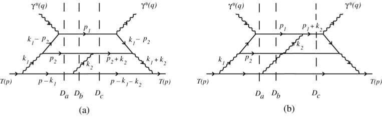
Figure 1: Two types of final state interactions. (a) Scattering of the antiquark ($p_{2}$ line), which in the aligned jet kinematics is part of the target dynamics. (b) Scattering of the current quark ($p_{1}$ line). For each LC time-ordered diagram, the potentially on-shell intermediate states corresponding to the denominators $D_{a},D_{b},D_{c}$ are denoted by dashed lines.

We recall that in LCPT the ‘$-$’ momentum component is not an independent variable, but is given by the on-shell condition, $k^{-}=(k_{\perp}^{2}+m^{2})/k^{+}$. Each propagating line has a factor $1/k^{+}$, and there is a denominator factor

$$D_{int}=\sum_{inc}k^{-}-\sum_{int}k^{-}+i\varepsilon$$ (7)

for each intermediate state, which measures the LC energy difference between the incoming and intermediate states. In Feynman gauge (which we use in this section) an imaginary part or discontinuity can arise only via the $i\varepsilon$ prescription in (7), when LC energy is conserved and the intermediate state is on-shell.

We consider the ‘aligned jet’ (or parton model) configuration [12], where the hard vertex is taken at zeroth order in the strong coupling: $\gamma^{*}{\rm q}\to{\rm q}$. In the aligned jet kinematics the momentum $p_{1}$ of the struck quark in Fig. 1 is the only one which grows in the Bjorken limit: $p_{1}^{-}\simeq 2\nu$, with $\vec{p}_{1\perp}$ independent of $\nu$. All momenta in Fig. 1 other than $q$ and $p_{1}$ remain finite in the Bjorken limit. The condition that the momentum fraction of the struck quark equals $x_{B}$ follows from the conservation of ‘$+$’ momentum, given that $p_{1}^{+}={\cal O}\left(1/\nu\right)$.

We recall (see, e.g., Eq. (A5) of Ref. [13]) that the virtual photon polarization vectors may be chosen as

$$\varepsilon(\lambda=\pm 1) = -\frac{1}{\sqrt{2}}(0,0,1,\pm i)$$

$$\varepsilon(\lambda=0) = \frac{Q}{\nu}(1,-1,0,0)$$ (8)

Since we take all lines (except the gauge bosons) in Fig. 1 to be scalars, the longitudinal photon coupling $\varepsilon(\lambda=0)\cdot(p_{1}+k_{1}-p_{2})\simeq Q$ dominates over the transverse ones in the Bjorken limit. The two longitudinal photon couplings together contribute a factor $Q^{2}$ to the forward amplitudes in Figs. 1a and 1b.

Both diagrams in Fig. 1 contain final state interactions between the $\gamma^{*}$ vertices. Only the three intermediate states indicated by dashed vertical lines can kinematically be on-shell and thus contribute to the discontinuity of the diagrams via the vanishing of the corresponding denominator $D_{a},\ D_{b}$ or $D_{c}$. We wish to ascertain whether the sum of these discontinuities gives a leading-twist contribution to the DIS cross section through the optical theorem (5). We use Feynman gauge in the following discussion. As we shall see in section 7 and Appendix C, the specific Feynman diagrams causing FSI effects in DIS actually depend on the gauge.

The three denominators of Fig. 1a are

$$D_{a} = q^{-}+p^{-}-p_{1}^{-}-p_{2}^{-}-(p-k_{1})^{-}$$

$$= 2\nu-\frac{p_{1\perp}^{2}+m^{2}}{p_{1}^{+}}+M-\frac{p_{2\perp}^{2}+m^{2}}{p_{2}^{+}}-\frac{k_{1\perp}^{2}+M^{2}}{M-k_{1}^{+}}$$

$$D_{b} = 2\nu-\frac{p_{1\perp}^{2}+m^{2}}{p_{1}^{+}}+M-\frac{p_{2\perp}^{2}+m^{2}}{p_{2}^{+}}-\frac{k_{2\perp}^{2}}{k_{2}^{+}}-\frac{(\vec{k}_{1\perp}+\vec{k}_{2\perp})^{2}+M^{2}}{M-k_{1}^{+}-k_{2}^{+}}$$

$$D_{c} = 2\nu-\frac{p_{1\perp}^{2}+m^{2}}{p_{1}^{+}}+M-\frac{(\vec{p}_{2\perp}+\vec{k}_{2\perp})^{2}+m^{2}}{p_{2}^{+}+k_{2}^{+}}-\frac{(\vec{k}_{1\perp}+\vec{k}_{2\perp})^{2}+M^{2}}{M-k_{1}^{+}-k_{2}^{+}}$$

and have the form

$$D_{a,b,c}=2\nu-\frac{p_{1\perp}^{2}+m^{2}}{p_{1}^{+}}+f_{a,b,c}$$ (10)

where $f_{a},f_{b},f_{c}$ are independent of $\nu$ in the aligned jet configuration. If we consider these denominators as functions of $p_{1}^{+}$ then the three conditions $D_{a,b,c}=0$ give to leading order the same value of $p_{1}^{+}$,

$$p_{1}^{+}=\frac{p_{1\perp}^{2}+m^{2}}{2\nu}\left[1+{\cal O}\left(\frac{1}{\nu}\right)\right]$$ (11)

All denominators and other factors in the LCPT expression of Fig. 1a except $D_{a},D_{b}$ and $D_{c}$ are insensitive (at leading order) to a relative change in $p_{1}^{+}$ of ${\cal O}\left(1/\nu\right)$. Thus, as far as the discontinuity of Fig. 1a is concerned, we can regard the other factors as constants in the $p_{1}^{+}$-integral containing the denominator poles,

$$\mbox{Disc(Fig. 1a)}\propto Q^{2}\,{\rm Disc}\int\frac{dp_{1}^{+}}{p_{1}^{+}}\frac{1}{(D_{a}+i\varepsilon)(D_{b}+i\varepsilon)(D_{c}+i\varepsilon)}$$ (12)

where the factor $Q^{2}$ stems from the photon couplings. All remaining factors in the proportionality are independent of $\nu$. Each of the three denominators in (12) gives a $\nu$-independent contribution to the discontinuity in the Bjorken limit. This means that each partial discontinuity contributes to the DIS cross section of Eq. (5) at the leading twist level, $\sigma(\gamma^{*}T\to X)\propto 1/Q^{2}$. However, as is easily seen, the contributions from the three poles which to leading order occur at the same value (11) of $p_{1}^{+}$ cancel at leading twist.

The above argument is generic and applies to arbitrarily complex diagrams having no interactions on the current quark line $p_{1}$. The remarkable fact that FSI between target spectators do not affect the DIS cross section only relies on the Bjorken limit, which as $\nu\to\infty$ provides an ‘infinite energy reservoir’ which compensates any target excitations.

The situation is quite different for diagrams like Fig. 1b where the current quark reinteracts. In (quasi-)elastic scattering of the current quark the momentum transfer $k_{2}^{+}\propto 1/\nu$. We may check explicitly that this range of momentum transfer indeed gives a leading-twist contribution to each partial discontinuity. The denominators are now of the form

$$D_{a} \simeq 2\nu-\frac{p_{1\perp}^{2}+m^{2}}{p_{1}^{+}}+g_{a}$$

$$D_{b} \simeq 2\nu-\frac{p_{1\perp}^{2}+m^{2}}{p_{1}^{+}}-\frac{k_{2\perp}^{2}}{k_{2}^{+}}+g_{b}$$ (13)

$$D_{c} \simeq 2\nu-\frac{(\vec{p}_{1\perp}+\vec{k}_{2\perp})^{2}+m^{2}}{p_{1}^{+}+k_{2}^{+}}+g_{c}$$

where $g_{a,b,c}$ are again independent of $\nu$. For example, picking up the $D_{a}=0$ pole in the $p_{1}^{+}$ integral we have

$$\mbox{Disc${}_{a}$(Fig. 1b)}\propto Q^{2}{p_{1}^{+}}{p_{1}^{-}}\,\int\frac{dk_{2}^{+}}{k_{2}^{+}(p_{1}^{+}+k_{2}^{+})}\frac{1}{D_{b}\,D_{c}}$$ (14)

where $p_{1}^{+}$ is given by (11) and the factor $p_{1}^{-}$ originates from the interaction in Feynman gauge.

Note that $D_{b}$ and $D_{c}$ are still of ${\cal O}\left(\nu\right)$ at the value (11) of $p_{1}^{+}$ for which $D_{a}=0$. The fact that the contributions from $D_{a}=0,\ D_{b}=0$ and $D_{c}=0$ thus occur at distinct values of $p_{1}^{+}$ means that they no longer cancel. ${\rm Disc}_{a}$ is independent of $\nu$ and hence contributes to the DIS cross section at leading twist. We conclude that rescattering of the current quark generally affects the cross section. In section 6 we shall demonstrate, in terms of an explicit perturbative example, that this conclusion is indeed correct.

Since the LC energy differences $D_{b,c}\propto\nu$ at $D_{a}=0$, the struck quark rescattering occurs on the light-cone, $y^{+}\sim{\cal O}\left(1/\nu\right)$. This rescattering is part of the dynamics described by the path-ordered exponential in the matrix element (S0.Ex2), where all $A^{+}$ fields are evaluated at the same LC time $y^{+}$. During its passage through the target the struck quark has no time to emit or absorb gluons, it only ‘samples’ the Coulomb field of the target. The rescattering nevertheless changes the transverse momentum of the quark and influences the cross section. This is analogous to the LPM effect [14], which suppresses the bremsstrahlung of a high energy electron in matter due to Coulomb rescattering within the formation time of the radiated photons.

4. The Glauber-Gribov Picture of Shadowing

DIS data on nuclear targets $A$ has shown that nuclear structure functions are suppressed for $x_{B}\buildrel<\over{{}_{\sim}}0.05$: $F_{2}^{A}(x_{B},Q^{2})<A\,F_{2}^{N}(x_{B},Q^{2})$ [10]. This is generally interpreted as a leading twist ‘shadowing’ effect, arising from quantum mechanical interference [9, 10]. The coherence length of the virtual photon in the target rest frame (6) is long at small $x_{B}$,

$$\frac{2\nu}{Q^{2}}=\frac{1}{Mx_{B}}=\langle y^{-}\rangle$$ (15)

as can also be seen from Eq. (S0.Ex2). Rescattering from different nucleons in the nucleus can thus interfere.

In the aligned jet kinematics the virtual photon fluctuates into a q${\rm\bar{q}}$ pair with limited transverse momentum, and the (struck) quark takes nearly all the longitudinal momentum of the photon. Using the notation of Fig. 1, where the initial q and ${\rm\bar{q}}$ momenta are denoted $p_{1}$ and $p_{2}-k_{1}$, respectively, we have

$$p_{1}^{-} \simeq 2\nu$$

$$p_{2}^{+}-k_{1}^{+} \simeq -Mx_{B}$$ (16)

$$\vec{p}_{1\perp}=-(\vec{p}_{2_{\perp}}-\vec{k}_{1_{\perp}}) \sim \Lambda_{QCD}$$

The (covariant) virtualities $p_{1}^{2}$ and $(p_{2}-k_{1})^{2}$ are limited. Hence $(p_{1}+p_{2}-k_{1})^{2}\sim p_{1}^{-}(p_{2}^{+}-k_{1}^{+})\sim-Q^{2}$ as required by momentum conservation. The virtual quark pair is put on-shell by a (total) momentum transfer $k$ from the target, with

$$k^{+}=p_{1}^{+}+p_{2}^{+}-q^{+}\simeq p_{2}^{+}+Mx_{B}$$ (17)

The DIS cross section is dominated by minimal transfers $k^{+}$, which for the final antiquark momentum gives

$$p_{2}^{+}\sim Mx_{B}$$ (18)

With this kinematics in mind the Glauber-Gribov picture of shadowing can be summarized as follows. At small $x_{B}$ the antiquark momentum $p_{2}^{-}\propto 1/x_{B}$ is large but the momentum transfer $k^{+}\sim Mx_{B}$ is small. The scattering will therefore have a diffractive component. In particular, the quark pair may scatter elastically on a ‘front’ nucleon $N_{1}$ in the nucleus before suffering an inelastic collision at a ‘back’ nucleon $N_{2}$, as indicated on the lhs of Fig. 2. The small momentum transfer $k^{+}$ at $N_{1}$ required to put the quark pair on-shell can be absorbed by the nuclear wave function. Hence this amplitude interferes with the amplitude for a single scattering on $N_{2}$ shown on the rhs of Fig. 2. The interference is destructive due to the imaginary nature of the Pomeron exchange amplitude at $N_{1}$ and the factor of $i$ resulting from the intermediate state between $N_{1}$ and $N_{2}$ going on-shell.

Figure 2: Glauber-Gribov shadowing involves interference between rescattering amplitudes.

This shadowing effect on the DIS cross section is not compatible with the cross section being determined by the parton probabilities ${\cal P}$ of Eq. (1). Since the Pomeron amplitude in Fig. 2 is imaginary it must involve on-shell intermediate states. But initial state interactions in the target before the virtual photon is absorbed cannot create on-shell intermediate states – they would constitute decay channels of the target. We conclude that Glauber-Gribov shadowing involves final state interactions and hence must be associated with the path ordered exponential in (S0.Ex2).

5. A Perturbative Example of Shadowing

We shall construct a perturbative example of the physics of Glauber-Gribov shadowing, which is simple enough to allow explicit expressions for the scattering amplitudes at small $x_{B}$. We use this example in section 6 to verify the general result of section 3 that final state interactions between target spectators do not affect the DIS cross section, whereas rescattering of the struck quark does.

In this section we use standard covariant perturbation theory in Feynman gauge of a scalar abelian gauge theory.

We consider the forward $\gamma^{*}T\to\gamma^{*}T$ amplitude of Fig. 3, the discontinuity of which gives a contribution to $\sigma(\gamma^{*}T)$ at order $\alpha\alpha_{s}^{4}$ via the optical theorem (5). Since we may assume the charges of the target $T$ and the ‘quark’ q to be distinct, we can focus on the gauge invariant set of diagrams in which the gluons are exchanged between the quark pair and the target. Each gluon $k_{i}$ can couple to either the q or the ${\rm\bar{q}}$ line, and all distinct permutations of the gluon vertices are included.

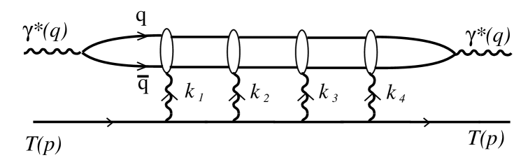
Figure 3: Forward $\gamma^{*}T\to\gamma^{*}T$ amplitude. All attachments of the exchanged gluons to the upper scalar loop are included, as well as topologically distinct permutations of the lower vertices on the target line.

Taking the discontinuity between gluons $k_{3}$ and $k_{4}$ gives a contribution which models the interference term of Fig. 2. The scattering on $N_{2}$ is given by single gluon exchange, while the Pomeron exchange on $N_{1}$ is modelled by two gluon exchange. The discontinuity between gluons $k_{2}$ and $k_{3}$ gives the square of the ‘Pomeron’ exchange amplitude. We calculate the one-, two- and three-gluon exchange amplitudes for $\gamma^{*}T\to{\rm q}{\rm\bar{q}}T$ explicitly for $x_{B}\ll 1$, making use of the results of Ref. [13] where a similar model was studied. Since the target $T$ is taken to be elementary this model does not have shadowing in the conventional sense described in section 4. It nevertheless demonstrates how final state interference effects reduce the DIS cross section.

We work in the target rest frame (6) and in the aligned jet kinematics of Eqs. (S0.Ex14) and (18). The Feynman gauge calculation is simplified by assuming a large target mass $M$. Hence the kinematic limit we consider is

$$2\nu\sim p_{1}^{-}\gg M\gg p_{2}^{-}\gg k_{i\perp},\ p_{2\perp},\ k_{i}^{-},\ m\gg k_{i}^{+},\ k^{+}=Mx_{B}+p_{2}^{+}$$ (19)

where $m$ is the mass of the q, ${\rm\bar{q}}$ quarks and $k=\sum_{i}k_{i}$ is the total momentum transfer from the target.

5.1 Single Gluon Exchange Amplitude $A$

The three Feynman diagrams are shown in Fig. 4. As in section 3 we use the virtual photon polarization vectors (8) and find that the dominant (leading twist) contribution comes from $\varepsilon(\lambda=0)\cdot p_{1}\simeq Q$. Diagram 4c is proportional to $\varepsilon\cdot(p+p^{\prime})$ and is thus non-leading. Diagram 4a involves the quark propagator

$$(p_{2}-k)^{2}-m^{2}\simeq p_{2}^{-}(p_{2}^{+}-k^{+})-(\vec{p}_{2\perp}-\vec{k}_{\perp})^{2}-m^{2}=-D(\vec{p}_{2\perp}-\vec{k}_{\perp})$$ (20)

where we used (17) and defined

$$D(\vec{p}_{\perp})\equiv p_{2}^{-}Mx_{B}+{p_{\perp}}^{2}+m^{2}$$ (21)

Similarly the quark propagator in diagram 4b gives $D(\vec{p}_{2\perp})$. The full amplitude in the limit (19) is

$$A(p_{2}^{-},\vec{p}_{2\perp},\vec{k}_{\perp})=\frac{2eg^{2}MQp_{2}^{-}}{k_{\perp}^{2}}\left[\frac{1}{D(\vec{p}_{2\perp})}-\frac{1}{D(\vec{p}_{2\perp}-\vec{k}_{\perp})}\right]$$ (22)

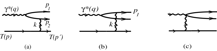
Figure 4: Single gluon exchange diagrams in scalar abelian theory.

We may readily verify that this contribution is of leading twist. The $\ell+T\to\ell^{\prime}+X$ DIS cross section is,

$$Q^{4}\frac{d\sigma}{dQ^{2}\,dx_{B}}=\frac{\alpha}{16\pi^{2}}\frac{1-y}{y^{2}}\frac{1}{2M\nu}\int\frac{dp_{2}^{-}}{p_{2}^{-}}\,\frac{d^{2}\vec{p}_{2\perp}}{(2\pi)^{2}}\,\frac{d^{2}\vec{k}_{\perp}}{(2\pi)^{2}}\,|A|^{2}$$ (23)

where $y=\nu/E_{\ell}$. The factor $Q^{2}$ in $|A|^{2}$ combines with $1/2M\nu$ in (23) to make the rhs independent of $Q^{2}$ in the Bjorken limit, when the soft momenta $\vec{k}_{\perp}$ and $p_{2}$ are integrated over any finite domain.

We also note that the dominant contribution to the DIS cross section at small $x_{B}$ comes from $p_{2}^{+}\sim Mx_{B}$ and $p_{2}^{-}\sim(p_{2\perp}^{2}+m^{2})/Mx_{B}$ as assumed in (18). To see this, note that the amplitude $A\propto p_{2}^{-}$ for $p_{2}^{-}\ll(p_{2\perp}^{2}+m^{2})/Mx_{B}$, while $A\propto 1/p_{2}^{-}$ for $p_{2}^{-}\gg(p_{2\perp}^{2}+m^{2})/Mx_{B}$.

Since $A\propto 1/k_{\perp}$ for $k_{\perp}\to 0$ the cross section (23) has a logarithmic singularity in this limit, which is regulated by the longitudinal momentum exchange at $k_{\perp}\sim k^{+}\sim Mx_{B}$. This logarithmic behavior occurs only at lowest order [15] and will not be relevant for our conclusions.

It is instructive to express the cross section also as an integral over the transverse distances $r_{\perp},R_{\perp}$ conjugate to $p_{2\perp},k_{\perp}$. Defining

$$\tilde{A}(p_{2}^{-},\vec{r}_{\perp},\vec{R}_{\perp})=\int\frac{d^{2}\vec{p}_{2\perp}}{(2\pi)^{2}}\,\frac{d^{2}\vec{k}_{\perp}}{(2\pi)^{2}}\,A(p_{2}^{-},\vec{p}_{2\perp},\vec{k}_{\perp})\exp\left(i\vec{r}_{\perp}\cdot\vec{p}_{2\perp}+i\vec{R}_{\perp}\cdot\vec{k}_{\perp}\right)$$ (24)

and using

$$V(m\,r_{\perp})\equiv\int\frac{d^{2}\vec{p}_{\perp}}{(2\pi)^{2}}\frac{e^{i\vec{r}_{\perp}\cdot\vec{p}_{\perp}}}{p_{\perp}^{2}+m^{2}}=\frac{1}{2\pi}K_{0}(m\,r_{\perp})$$ (25)

where $K_{0}$ is a Bessel function, and

$$W(\vec{r}_{\perp},\vec{R}_{\perp})\equiv\int\frac{d^{2}\vec{k}_{\perp}}{(2\pi)^{2}}\frac{1-e^{i\vec{r}_{\perp}\cdot\vec{k}_{\perp}}}{k_{\perp}^{2}}e^{i\vec{R}_{\perp}\cdot\vec{k}_{\perp}}=\frac{1}{2\pi}\log\left(\frac{|\vec{R}_{\perp}+\vec{r}_{\perp}|}{R_{\perp}}\right)$$ (26)

we get from (22),

$$\tilde{A}(p_{2}^{-},\vec{r}_{\perp},\vec{R}_{\perp})=2eg^{2}MQp_{2}^{-}\,V(m_{||}r_{\perp})W(\vec{r}_{\perp},\vec{R}_{\perp})$$ (27)

where

$$m_{||}^{2}=p_{2}^{-}Mx_{B}+m^{2}$$ (28)

The contribution (23) to the DIS cross section can then be expressed as

$$Q^{4}\frac{d\sigma}{dQ^{2}\,dx_{B}} = \frac{\alpha^{2}\alpha_{s}^{2}}{\pi^{3}}\frac{1-y}{y^{2}}x_{B}M^{2}\int dp_{2}^{-}\frac{p_{2}^{-}}{\left(p_{2}^{-}Mx_{B}+m^{2}\right)^{2}}$$ (29)

$$\times \int d^{2}\vec{u}_{\perp}d^{2}\vec{U}_{\perp}\left[K_{0}(u_{\perp})\log\left(\frac{|\vec{U}_{\perp}+\vec{u}_{\perp}|}{U_{\perp}}\right)\right]^{2}$$

Here the dimensionless integration variables were defined as $\vec{u}_{\perp}=\vec{r}_{\perp}m_{||}$ and $\vec{U}_{\perp}=\vec{R}_{\perp}m_{||}$, showing that the typical transverse distances $\vec{r}_{\perp},\vec{R}_{\perp}$ scale as $1/m_{||}$. The $p_{2}^{-}$ integral in (29) is logarithmic at large $p_{2}^{-}>m^{2}/Mx_{B}$, where the aligned jet $\gamma^{*}{\rm q}\to{\rm q}$ subprocess turns into $\gamma^{*}\gamma\to{\rm q}{\rm\bar{q}}$ [13].

5.2 Two-Gluon Exchange Amplitude $B$ Fig. 5 shows two of the altogether six two-gluon exchange diagrams which give leading contributions to the $\gamma^{*}T\to{\rm q}{\rm\bar{q}}T$ amplitude for $x_{B}\ll 1$ in Feynman gauge. Diagrams with 4-point vertices (cf. Fig. 4c) are again suppressed in this gauge. We illustrate the calculation of this one-loop amplitude using the diagrams of Fig. 5.

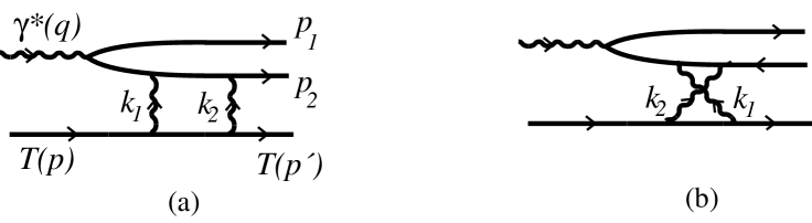
Figure 5: Double gluon exchange diagrams. In Feynman gauge four more diagrams contribute at leading order, where one or both of the exchanged gluons attach to the quark ($p_{1}$) line.

Our assumption (19) of a large target mass $M$ simplifies the loop integral by suppressing the $k_{i}^{0}$ momentum components. For the overall exchange we find from the mass-shell condition $p^{\prime 2}=(p-k)^{2}=M^{2}$ that

$$k^{0}=k_{1}^{0}+k_{2}^{0}=-\frac{k_{\perp}^{2}}{2M}\ll k^{\pm},\ k_{\perp}$$ (30)

The corresponding suppression for the loop momentum $k_{1}^{0}\simeq-k_{2}^{0}$ results from the sum of the uncrossed and crossed gluon attachments to the target line in Fig. 5,

$$(-ig\,2M)^{2}\left[\frac{i}{(p-k_{1})^{2}-M^{2}+i\varepsilon}+\frac{i}{(p-k_{2})^{2}-M^{2}+i\varepsilon}\right]$$

$$\simeq 2ig^{2}M\left(\frac{1}{k_{1}^{0}-i\varepsilon}+\frac{1}{k_{2}^{0}-i\varepsilon}\right)\simeq 2ig^{2}M\ 2\pi i\delta(k_{1}^{0})$$ (31)

Making use of Eqs. (20) and (31) we find

$$B(5a)+B(5b) = -\frac{2eg^{4}MQ\,p_{2}^{-}}{D(\vec{p}_{2\perp}-\vec{k}_{\perp})}\int\frac{d^{2}\vec{k}_{2\perp}\,dk_{2}^{+}}{(2\pi)^{3}}\frac{1}{\vec{k}_{1}^{2}\vec{k}_{2}^{2}}$$ (32)

$$\times \frac{1}{k_{2}^{+}-(2\vec{p}_{2\perp}\cdot\vec{k}_{2\perp}-\vec{k}_{2}^{2})/p_{2}^{-}-i\varepsilon}$$

Symmetrizing the integrand in $\vec{k}_{1}\leftrightarrow\vec{k}_{2}$ and recalling (17) the last factor becomes

$$\frac{1}{2}\left[\frac{1}{k_{2}^{+}-(2\vec{p}_{2\perp}\cdot\vec{k}_{2\perp}-\vec{k}_{2}^{2})/p_{2}^{-}-i\varepsilon}-\frac{1}{k_{2}^{+}-k^{+}+(2\vec{p}_{2\perp}\cdot\vec{k}_{1\perp}-\vec{k}_{1}^{2})/p_{2}^{-}+i\varepsilon}\right]$$

(33)

$$\simeq i\pi\delta(k_{2}^{+})\mbox{\hskip 284.52756pt}$$

Thus

$$B(5a)+B(5b)=-\frac{ieg^{4}MQ\,p_{2}^{-}}{D(\vec{p}_{2\perp}-\vec{k}_{\perp})}\int\frac{d^{2}\vec{k}_{2\perp}}{(2\pi)^{2}}\,\frac{1}{k_{1\perp}^{2}\,k_{2\perp}^{2}}$$ (34)

Adding the contributions from the remaining four diagrams we find for the full two-gluon exchange amplitude

$$B(p_{2}^{-},\vec{p}_{2\perp},\vec{k}_{\perp}) = -ieg^{4}MQp_{2}^{-}\int\frac{d^{2}\vec{k}_{1\perp}}{(2\pi)^{2}}\ \frac{1}{k_{1\perp}^{2}k_{2\perp}^{2}}$$

$$\times \left[\frac{1}{D(\vec{p}_{2\perp})}-\frac{1}{D(\vec{p}_{2\perp}-\vec{k}_{1\perp})}-\frac{1}{D(\vec{p}_{2\perp}-\vec{k}_{2\perp})}+\frac{1}{D(\vec{p}_{2\perp}-\vec{k}_{\perp})}\right]$$

where $\vec{k}_{2\perp}=\vec{k}_{\perp}-\vec{k}_{1\perp}$. We note that the amplitude is fully imaginary as required by crossing symmetry, since $B\propto p_{2}^{-}$ as $p_{2}^{-}\to\infty$ and two gluon exchange has even charge conjugation. Thus our model captures the essential features of Pomeron exchange. We note also that $B(p_{2}^{-},\vec{p}_{2\perp},\vec{k}_{\perp})\propto\log k_{\perp}$ for $k_{\perp}\to 0$. In contrast to the single gluon exchange contribution to the DIS cross section, the square of (S0.Ex22) can thus be safely integrated over $k_{\perp}$ and (for $m\neq 0$) over $p_{2}^{-}$.

Due to conservation of the transverse distances $\vec{r}_{\perp},\vec{R}_{\perp}$ in the peripheral scattering, the Fourier transform (24) returns the simple form

$$\tilde{B}(p_{2}^{-},\vec{r}_{\perp},\vec{R}_{\perp})=-ieg^{4}MQp_{2}^{-}V(m_{||}r_{\perp})W^{2}(\vec{r}_{\perp},\vec{R}_{\perp})=\frac{-ig^{2}}{2!}W\tilde{A}$$ (36)

where we used (25) and (26).

We stress that in the $x_{B}\to 0$ limit, the amplitude $B$ is dominated by the configuration where the intermediate state between the two exchanges is on-shell. This can be seen by calculating $B$ in LC time-ordered perturbation theory, where this intermediate state is associated with a vanishing denominator (7). Alternatively, we may note that since the real part of $B$ is suppressed in the $x_{B}\to 0$ limit the full amplitude is (via the optical theorem) given by its discontinuity. This is true in all gauges since $B$ is gauge invariant.

5.3 Three-Gluon Exchange Amplitude $C$

No qualitatively new aspects appear in the calculation of this two-loop amplitude. Permuting the attachments of the three gluons on the target line one finds in analogy to (31) that $k_{i}^{0}\simeq 0$ for all exchanges $(i=1,2,3)$. Similarly the $k_{i}^{+}$ integrations are simply evaluated after symmetrizations analogous to (S0.Ex20). The final expression in momentum space is

$$C(p_{2}^{-},\vec{p}_{2\perp},\vec{k}_{\perp})=-\frac{1}{3}eg^{6}MQp_{2}^{-}\int\frac{d^{2}\vec{k}_{1\perp}}{(2\pi)^{2}}\frac{d^{2}\vec{k}_{2\perp}}{(2\pi)^{2}}\ \frac{1}{\vec{k}_{1\perp}^{2}\,\vec{k}_{2\perp}^{2}\,\vec{k}_{3\perp}^{2}}\mbox{\hskip 99.58464pt}$$ (37)

$$\times\left[\frac{1}{D(\vec{p}_{2\perp})}-\frac{3}{D(\vec{p}_{2\perp}-\vec{k}_{1\perp})}+\frac{3}{D(\vec{p}_{2\perp}-\vec{k}_{1\perp}-\vec{k}_{2\perp})}-\frac{1}{D(\vec{p}_{2\perp}-\vec{k}_{\perp})}\right]$$

where $\vec{k}_{3\perp}=\vec{k}_{\perp}-\vec{k}_{1\perp}-\vec{k}_{2\perp}$.

The Fourier transform (24) gives the amplitude in transverse coordinate space as

$$\tilde{C}(p_{2}^{-},\vec{r}_{\perp},\vec{R}_{\perp})=-\frac{1}{3}eg^{6}MQp_{2}^{-}V(m_{||}r_{\perp})W^{3}(\vec{r}_{\perp},\vec{R}_{\perp})=\frac{(-ig^{2})^{2}}{3!}W^{2}\tilde{A}$$ (38)

Similarly to the $B$ amplitude, $C$ arises from the intermediate states between the rescatterings being on-shell in the $x_{B}\to 0$ limit. Again this must hold also in LC gauge. Since in the two-loop case there are two consequtive intermediate states, $C$ is purely real.

From the expressions (27), (36) and (38), it is apparent that the sum of gluon-exchange amplitudes exponentiates,

$$\tilde{\cal M}(p_{2}^{-},\vec{r}_{\perp},\vec{R}_{\perp})=\tilde{A}+\tilde{B}+\tilde{C}\ldots=-2ieMQp_{2}^{-}V\left[1-\exp(-ig^{2}W)\right]$$ (39)

As noted at the beginning of this section, we have assumed the charges of the quark and target lines to be distinct. This allows us to restrict our analysis to the subclass of Feynman diagrams considered above, since diagrams with different powers of the charges cannot cancel in the DIS cross section. However, we should note that at the level of three gluon exchanges there are new types of diagrams which have the same charge dependence as $C$ in Eq. (37). For example, one of the three gluons may be exchanged between the quarks while another forms a loop on the target line. The $k_{\perp}$-dependence of this contribution would differ from that of (37). We do not further consider such contributions.

6. Effects of Rescattering on the DIS Cross Section

We now use our perturbative amplitudes to demonstrate that final-state rescattering of the struck quark affects the DIS cross section. In the previous section we used covariant (rather than time-ordered) perturbation theory, and thus did not distinguish between initial (ISI) and final (FSI) state interactions. However, diagrams involving rescattering of the struck quark necessarily are FSI because the exchanged gluon couples to the struck quark ($p_{1}$) line after the virtual photon. We shall see that precisely such diagrams contribute to the cross section.

We consider the DIS cross section (23) expressed as a sum over the transverse distances $\vec{r}_{\perp},\vec{R}_{\perp}$ defined in (24),

$$Q^{4}\frac{d\sigma}{dQ^{2}\,dx_{B}}=\frac{\alpha}{16\pi^{2}}\frac{1-y}{y^{2}}\frac{1}{2M\nu}\int\frac{dp_{2}^{-}}{p_{2}^{-}}\,d^{2}\vec{r}_{\perp}\,d^{2}\vec{R}_{\perp}\,|\tilde{\cal M}|^{2}$$ (40)

where

$$|\tilde{\cal M}(p_{2}^{-},\vec{r}_{\perp},\vec{R}_{\perp})|=\left|\frac{\sin\left[g^{2}\,W(\vec{r}_{\perp},\vec{R}_{\perp})/2\right]}{g^{2}\,W(\vec{r}_{\perp},\vec{R}_{\perp})/2}\tilde{A}(p_{2}^{-},\vec{r}_{\perp},\vec{R}_{\perp})\right|$$ (41)

is the resummed amplitude (39) and $V,W$ are given in Eqs. (25) and (26), respectively.

The fact that the coefficient of $\tilde{A}$ in (41) is less than unity for all $\vec{r}_{\perp},\vec{R}_{\perp}$ shows that the rescattering corrections included in $\tilde{\cal M}$ reduce the cross section. This effect agrees with the Glauber-Gribov picture of DIS shadowing and must be present also in LC gauge (see section 7).

The forward $\gamma^{*}T\to\gamma^{*}T$ amplitude in Fig. 3 can also be cut through some of the gluon lines, corresponding to final states with real gluons. Such contributions have, however, a different target mass $M$ dependence (cf. Eq. (30)). Similar arguments suggest that other contributions, even if they are of the same order in the coupling constants, cannot change the conclusion that the DIS cross section is influenced by final state interactions.

In section 3 we gave a general argument (in Feynman gauge) which showed that final state interactions between target spectators cannot influence the DIS cross section (cf. Fig. 1a). We shall now check this statement using our perturbative amplitudes.

In the aligned jet kinematics the antiquark belongs to the target system. We thus consider the subset of diagrams like Figs. 4a and 5 where all exchanged gluons attach to the ${\rm\bar{q}}$ ($p_{2}$) line. One can easily verify that this subset of diagrams is gauge invariant in the class of covariant gauges in our kinematic limit (19). The corresponding sum of cuts in Fig. 3 is then proportional to

$$S_{{\rm\bar{q}}}(p_{2}^{-},\vec{p}_{2\perp},\vec{k}_{\perp})=|B_{{\rm\bar{q}}}|^{2}+2{\rm Re}(A_{{\rm\bar{q}}}\,C_{{\rm\bar{q}}}^{*})$$ (42)

where the subscript ${\rm\bar{q}}$ indicates the subset of diagrams.

Diagrams where all gluons attach to the antiquark line can involve both ISI and FSI. Since the two-gluon exchange contribution (34) is imaginary it must, however, involve rescattering of on-shell intermediate states which can only arise after the virtual photon has been absorbed. Similarly the (real) three-gluon exchange amplitude $C$ (37) involves double rescattering of on-shell states. Hence all our amplitudes (except the Born term $A$) involve FSI.

It is straightforward to identify the $A_{{\rm\bar{q}}},B_{{\rm\bar{q}}},C_{{\rm\bar{q}}}$ contributions to the expressions (22), (S0.Ex22), (37) of the full one-, two- and three-gluon exchange amplitudes in momentum space. According to Eq. (20) the antiquark propagator next to the virtual photon vertex gives a denominator $D(\vec{p}_{2\perp}-\vec{k}_{\perp})$ for all diagrams in our subset. This factor appears explicitly in each amplitude. Dimensionally regularizing the logarithmic infrared divergencies at $k_{i\perp}=0$ we thus find

$$S_{{\rm\bar{q}}}(p_{2}^{-},\vec{p}_{2\perp},\vec{k}_{\perp})=\left[\frac{eg^{4}MQp_{2}^{-}}{(2\pi)^{2}D(\vec{p}_{2\perp}-\vec{k}_{\perp})}\right]^{2}\left\{\left[R_{2}(k_{\perp})\right]^{2}-\frac{4}{3}R_{13}(k_{\perp})\right\}$$ (43)

where

$$R_{2}(k_{\perp}) = \int\frac{d^{D}\vec{k}_{1\perp}}{k_{1\perp}^{2}(\vec{k}_{\perp}-\vec{k}_{1\perp})^{2}}=\frac{\pi^{D/2}}{k_{\perp}^{4-D}}\frac{\left[\Gamma\left(\frac{D}{2}-1\right)\right]^{2}\Gamma\left(2-\frac{D}{2}\right)}{\Gamma\left(D-2\right)}$$

$$R_{13}(k_{\perp}) = \frac{1}{k_{\perp}^{2}}\int\frac{d^{D}\vec{k}_{1\perp}\ d^{D}\vec{k}_{2\perp}}{k_{1\perp}^{2}k_{2\perp}^{2}(\vec{k}_{\perp}-\vec{k}_{1\perp}-\vec{k}_{2\perp})^{2}}=\frac{\pi^{D}}{k_{\perp}^{8-2D}}\frac{\left[\Gamma\left(\frac{D}{2}-1\right)\right]^{3}\Gamma\left(3-D\right)}{\Gamma\left(\frac{3D}{2}-3\right)}$$

Expanding $R_{2}$ and $R_{13}$ around $D=2$ gives

$$R_{2}(k_{\perp}) = \frac{\pi^{D/2}}{k_{\perp}^{4-D}}\left\{\frac{4}{D-2}+2\gamma+\frac{1}{12}\left(6\gamma^{2}-\pi^{2}\right)\left(D-2\right)+\right.$$

$$+ \left.\frac{1}{24}\left[2\gamma^{3}-\gamma\pi^{2}-14\psi^{(2)}(1)\right]\left(D-2\right)^{2}+{\cal O}\left[(D-2)^{3}\right]\right\}\ ,$$

$$R_{13}(k_{\perp}) = \frac{\pi^{D}}{k_{\perp}^{8-2D}}\left\{\frac{12}{\left(D-2\right)^{2}}+\frac{12\gamma}{D-2}+\left(6\gamma^{2}-\frac{\pi^{2}}{2}\right)+\right.$$

$$+ \left.\frac{1}{2}\left[4\gamma^{3}-\gamma\pi^{2}-16\psi^{(2)}(1)\right]\left(D-2\right)+{\cal O}\left[(D-2)^{2}\right]\right\}\ ,$$

where $\gamma\simeq 0.577$ is Euler’s constant and $\psi^{(n)}(z)$ is the $(n+1)^{\rm th}$ logarithmic derivative of the gamma function with $\psi^{(2)}(1)\simeq-2.40$. Hence

$$\left[R_{2}(k_{\perp})\right]^{2}-\frac{4}{3}R_{13}(k_{\perp})=\frac{\pi^{D}}{k_{\perp}^{8-2D}}\,6\psi^{(2)}(1)\left(D-2\right)+{\cal O}\left[(D-2)^{2}\right]$$ (46)

vanishes at $D=2$. Thus FSI between the target spectators do not change the DIS cross section.

We conclude that in covariant gauges, only final state interactions which involve rescatterings of the current quark affect the DIS cross section.

7. Light-Cone Gauge $A^{+}=0$

We have seen that in a covariant gauge, the DIS cross section is influenced by final-state interactions of the struck quark in the target. This soft physics is contained in the path-ordered exponential of the matrix element (S0.Ex2) in a general gauge and appears to vanish in LC gauge, $n\cdot A=A^{+}=0$.

However, as we have seen in section 5 the amplitudes $B$ and $C$ arise from on-shell intermediate states in the $x_{B}\to 0$ limit. Thus in (40) the contribution of $|\tilde{\cal M}|^{2}$, whose expansion starts as $|\tilde{B}|^{2}+2\tilde{A}\tilde{C}$, also arises purely from on-shell intermediate states. The presence of such on-shell states is gauge independent and they can only occur in the final state. We conclude that the DIS cross section is influenced by final state interactions in all gauges. Thus parton distributions cannot be fully determined by parton probabilities in the target.

Let us now discuss some features inherent to the LC gauge preventing parton distributions from being probabilities, in other words making the expression (S0.Ex2) for $f_{{\rm q}/N}$ incorrect in LC gauge. It turns out that terms which are next-to-leading corrections in a general gauge cannot be ignored in LC gauge. To see this, it is helpful to recall how the exponential arises from perturbative diagrams.

As explained in Ref. [8] each quark field is associated with an ordered exponential

$$[A^{+}]\equiv{\rm P}\exp\left[ig\int_{0}^{\infty}dy^{-}A^{+}(y^{-})\right]$$ (47)

where the gauge field $A^{+}$ is evaluated on the light-cone, $y^{+}=y_{\perp}=0$. This factor arises from the interactions of the struck quark as it moves through the target. While the path in (47) extends to infinity, there is a partial cancellation between the quark fields in the matrix element (S0.Ex2) leaving a path of length $y^{-}\sim 1/Mx_{B}$ equal to the coherence length of the virtual photon. Only interactions within this LC distance can influence the cross section.

Expanding the exponential (47) gives

$$[A^{+}] = 1+ig\int_{0}^{\infty}dy_{1}^{-}A^{+}(y_{1}^{-})\left[1+ig\int_{y_{1}^{-}}^{\infty}dy_{2}^{-}A^{+}(y_{2}^{-})+\ldots\right]$$

$$= 1+g\int_{-\infty}^{\infty}\frac{dk_{1}^{+}}{2\pi}\frac{\tilde{A}^{+}(k_{1}^{+})}{k_{1}^{+}-i\varepsilon}+g^{2}\int_{-\infty}^{\infty}\frac{dk_{1}^{+}dk_{2}^{+}}{(2\pi)^{2}}\frac{\tilde{A}^{+}(k_{1}^{+})\tilde{A}^{+}(k_{2}^{+})}{(k_{1}^{+}+k_{2}^{+}-i\varepsilon)(k_{2}^{+}-i\varepsilon)}+\ldots$$

where

$$A^{+}(y^{-})=\int_{-\infty}^{\infty}\frac{dk^{+}}{2\pi}\tilde{A}^{+}(k^{+})\exp(-ik^{+}y^{-})$$ (49)

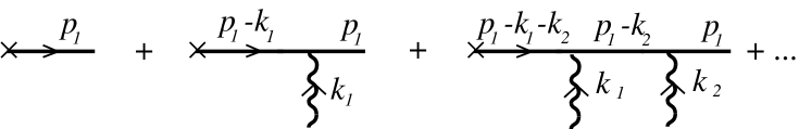
Figure 6: Scattering of the struck quark on the gauge field of the target which gives rise to the ordered exponential (47).

The terms in the expansion (S0.Ex32) arise from the perturbative diagrams of Fig. 6, where the cross indicates the virtual photon vertex. The struck quark momentum is asymptotically large, $p_{1}^{-}\to\infty$, implying that the quark moves along the light-cone $y^{+}=y_{\perp}=0$. The two-gluon exchange term in Fig. 6 is given by

$$(ig)^{2}i^{2}\frac{p_{1}^{-}\tilde{A}^{+}(k_{1}^{+})\,p_{1}^{-}\tilde{A}^{+}(k_{2}^{+})}{\left[-p_{1}^{-}(k_{1}^{+}+k_{2}^{+})+i\varepsilon\right](-p_{1}^{-}k_{2}^{+}+i\varepsilon)}=g^{2}\frac{\tilde{A}^{+}(k_{1}^{+})\tilde{A}^{+}(k_{2}^{+})}{(k_{1}^{+}+k_{2}^{+}-i\varepsilon)(k_{2}^{+}-i\varepsilon)}$$ (50)

Thus we find equivalence to the expression (S0.Ex32) by approximating $(2p_{1}-k_{2})\cdot\tilde{A}(k_{2}^{+})\simeq p_{1}^{-}\tilde{A}^{+}(k_{2}^{+})$, i.e., by keeping only the asymptotically large component of $p_{1}$. This is correct in all gauges except $A^{+}=0$, where this ‘leading’ term actually vanishes.

Neglecting the dependence of the matrix element (S0.Ex2) on the gauge field $\tilde{A}(k^{+})$ in LC gauge is equivalent to assuming that interactions of the struck quark with the gauge field such as $(2\vec{p}_{1}-\vec{k}_{2})_{\perp}\cdot\vec{{\tilde{A}}}_{\perp}$ do not contribute at leading twist. The following example shows how this assumption can fail.

As a simple illustration of how the high energy and LC gauge limit can fail to commute we consider the elastic process ${\rm q}(p_{1}-k)\,T(p)\to{\rm q}(p_{1})\,T(p-k)$, where $p=(M,M,\vec{0}_{\perp})$ and $p_{1}^{-}\to\infty$ at fixed $p_{1\perp},k_{\perp}$. Momentum conservation implies

$$k^{+} = \frac{(2\vec{p}_{1\perp}-\vec{k}_{\perp})\cdot\vec{k}_{\perp}}{p_{1}^{-}}\to 0$$

$$k^{-} = -\frac{k_{\perp}^{2}}{M}\ \ \ \mbox{fixed}$$ (51)

The interaction of the gauge field with the quark is given by $(-ig)(2p_{1}-k)_{\mu}\cdot d^{\mu\nu}(k)$. In Feynman gauge the propagator is $d_{F}^{\mu\nu}(k)=-ig^{\mu\nu}/(k^{2}+i\varepsilon)$ and the coupling is dominated by $-igp_{1}^{-}\,d_{F}^{+-}(k)$, which is analogous to the interaction (50) in the ordered exponential. The elastic amplitude

$$A({\rm q}T\to{\rm q}T)=-2g^{2}M\frac{p_{1}^{-}}{k_{\perp}^{2}}$$ (52)

is thus $\propto p_{1}^{-}$ as befits Coulomb exchange.

In LC gauge the propagator (4) satisfies $d_{LC}^{+\nu}(k)=0$, hence the $p_{1}^{-}$ component does not contribute. Yet the elastic amplitude is gauge independent and must still be given by (52). The absence of the factor $p_{1}^{-}$ in the numerator coupling is in fact compensated by the factor $k^{+}\propto 1/p_{1}^{-}$ in the denominator of the LC gauge propagator (4). The dominant contribution is from $-(2\vec{p}_{1}-\vec{k})^{\perp}\cdot d^{-\perp}(k)$ and the result indeed agrees with (52).

Note that if we had kept only the $d^{+\nu}(k)$ part of the gauge propagator in the high energy limit and then chosen LC gauge the elastic scattering amplitude would have seemed to vanish. This incorrect result is analogous to the apparent absence of rescattering effects in the matrix element (S0.Ex2) for $A^{+}=0$.

In the Feynman gauge calculation of section 5 we saw that the reinteractions of the struck quark with the target are essentially elastic, the intermediate states being on-shell in the $x_{B}\to 0$ limit. It is thus not surprising that the calculation of the scattering amplitudes in LC gauge has many features in common with the elastic scattering example above. Details of the calculation of the one-loop and two-loop amplitudes $B$ and $C$ (S0.Ex22) and (37) in LC gauge are given in the Appendices.

In LC gauge the Feynman rules must be supplemented with a prescription for the $k^{+}=0$ pole of the propagator (4). Three prescriptions that have been studied in the literature [11, 16, 17] are given in Eq. (64) of Appendix A. The contributions of the individual diagrams shown in Fig. 7 for the one-loop amplitude $B$ depend on the prescription. However, the $k_{i}^{+}=0$ poles cancel when all diagrams are added. Their sum is thus prescription independent and agrees with the Feynman gauge result (S0.Ex22). We verify the prescription independence of the two-loop amplitude $C$ in Appendix B. A consistent procedure for regulating the spurious poles is also discussed there.

As we have already emphasized, final state interactions (FSI) modify the DIS cross section also in LC gauge due to the presence of on-shell intermediate states between the rescatterings in the amplitudes $B$ and $C$. However, while in Feynman gauge it is the rescattering of the struck quark $p_{1}$ which affects the cross section, in LC gauge those rescatterings actually do not contribute. Indeed, we show in Appendix C that contributions from diagrams like Fig. 7c and 8b to the individual amplitudes cancel in the cross section. Thus in LC gauge, independently of the prescription, the cross section is modified by FSI occurring on the antiquark $p_{2}$, i.e., within the target system. Choosing the $A^{+}=0$ gauge shifts the rescatterings of the quark present in Feynman gauge to rescatterings of the antiquark. As also shown in Appendix C, in LC gauge the partial amplitude where only attachments to $p_{2}$ are kept equals the full amplitude, up to a phase factor. Which particle actually scatters in the quark-antiquark system depends on the gauge, but the presence of on-shell intermediate states does not.

Subtleties can appear when using the Kovchegov (K) prescription (see Eq. (64)), since the imaginary part arising from a physical cut can be changed by the imaginary part created by the prescription itself. The ${\rm K}$ prescription simulates the physics of the rescattering corrections by introducing an external gauge field into the dynamics. Unlike the Principal Value (PV) or Mandelstam-Leibbrandt prescription, the K prescription is not causal, and thus it would normally not be used for solving the bound state problem and light-cone wave functions of an isolated hadron in QCD. The solutions for the light-cone wave function of the target hadron in the presence of an external gauge field can have complex phases. This is apparently the way in which the light-cone wave functions of a nucleus in the Kovchegov light-cone gauge prescription mimic the effects of rescattering of the fast quark and the Glauber-Gribov shadowing modifications of the structure functions. If this picture could be validated, the Kovchegov LC gauge prescription would give a framework in which $\sigma_{DIS}$ is fully determined by the target LC wavefunction, solved in the presence of an external field.

8. Conclusions

We have found that final state Coulomb rescattering in the target, within the coherence length $2\nu/Q^{2}=1/Mx_{B}$ of the hard process, influences the $\ell N\to\ell^{\prime}X$ DIS cross section. In particular, diffractive scattering of the outgoing quark-pair on target spectators is a coherent effect which is not included in the light-front wave functions, even in light-cone gauge. Such effects modify the contributions of the individual target partons, implying that the DIS cross section is not fully given by the parton probabilities of the initial state. These coherent effects are reminiscent of the LPM effect [14], which suppresses the bremsstrahlung of a high energy electron in matter due to Coulomb rescattering of the electron within the formation time of its radiated photons.

Our analysis, when interpreted in frames with $q^{+}>0,$ also supports the color dipole description of deep inelastic lepton scattering at small $x$. Even in the case of the aligned jet configurations, one can understand DIS as due to the coherent color gauge interactions of the incoming quark-pair state of the photon interacting first coherently and finally incoherently in the target.

Our analysis in light-cone gauge resembles the “covariant parton model” of Landshoff, Polkinghorne and Short [18, 19] in the target rest frame. In this description of small $x$ DIS, the virtual photon with positive $q^{+}$ first splits into the pair $p_{1}$ and $p_{2}$. The aligned quark $p_{1}$ has no final state interactions. However, the antiquark line $p_{2}$ can interact in the target with an effective energy $\hat{s}\propto{k_{\perp}^{2}/x}$ while staying close to its mass shell. Thus at small $x$ and large $\hat{s}$, the antiquark $p_{2}$ line can first multiple scatter in the target via pomeron and Reggeon exchange, and then finally scatter inelastically or be annihilated. The DIS cross section can thus be written as an integral of the $\sigma(\bar{q}p\to X)$ cross section over the $p_{2}$ virtuality. In this way, the diffractive scattering of the antiquark in the nucleus gives rise to the shadowing of the nuclear cross section $\sigma(\bar{q}A\to X)$ [4].

Our results do not contradict the QCD factorization theorem [8] for inclusive reactions in a general gauge. However, they show that the apparent equivalence between the DIS cross section and the target parton probabilities (1) suggested by the forward matrix element (S0.Ex2) in $A^{+}=0$ gauge is incorrect. The $A_{\perp}$ components of the gauge field give leading twist contributions in LC gauge.

Our investigation was triggered by the fact that the physically plausible and phenomenologically successful Glauber-Gribov description of DIS shadowing [9, 10] implies that final state interactions influence the DIS cross section. The physics of shadowing is associated with final state diffractive scattering rather than with the (real) light-cone wave function of the target. There remains the possibility of incorporating shadowing in the target wave function by solving it under the specific boundary conditions implied by the Kovchegov LC gauge prescription [17].

Our analysis is consistent with the standard Operator Product Expansion. Hence the usual sum rules of the parton distributions remain valid in spite of the rescattering (shadowing) physics. We have not estimated the quantitative importance of the rescattering effects on $\sigma_{DIS}$, but it is natural to expect that they are more prominent at small values of $x_{B}$ where the coherence length is long. In particular, diffractive DIS is related to shadowing and is apparently generated by rescattering contributions.

Acknowledgements. We wish to thank G. Bodwin, T. Binoth, J. D. Bjorken, M. Burkardt, J. Collins, L. Frankfurt, A. Hebecker, G. Heinrich, Y. Kovchegov, L. Mankiewicz and M. Strikman for useful discussions. SJB and PH are grateful for the hospitality and support of the Institute for Nuclear Theory at the University of Washington during the completion of this work.

APPENDIX

A. One-loop calculation in $A^{+}=0$ gauge.

In this Appendix we present the calculation of the two-gluon exchange amplitude $B$ (S0.Ex22) in light-cone $n\cdot A=A^{+}=0$ gauge of a scalar abelian theory. We shall take the target mass to be of the order of the transverse momenta, i.e., rather than (19), we here consider the kinematic limit

$$2\nu\sim p_{1}^{-}\gg p_{2}^{-}\gg k_{i\perp},\ p_{2\perp},\ k_{i}^{-},\ m,\ M\gg\ k_{i}^{+},\ k^{+}=Mx_{B}+p_{2}^{+}$$ (53)

and show that the expression for the amplitude remains the same.

Figure 7: Diagrams that can give leading order contributions to the one-loop amplitude $B$ in $A^{+}=0$ gauge.

Leading contributions to the amplitude can come from diagrams $B_{a}\ldots B_{e}$ of Fig. 7. The factors associated with the gluon propagators are approximated as

$$(p+p^{\prime})^{\mu}d_{\mu\nu}(k)(2l+k)^{\nu}\simeq i\frac{2M}{k_{\perp}^{2}k^{+}}\left[D(k+l)-D(l)\right]$$ (54)

where only the $d^{-\perp}$ part of the propagator (4) contributes, and the function $D(p)\equiv D(\vec{p}_{\perp})$ is defined in (21). Similarly, the factor from the four-leg scalar abelian vertex simplifies to

$$(2p-k_{1})^{\mu}d_{\mu\nu}(k_{1})d^{\mu^{\prime}\nu}(k_{2})(2p^{\prime}+k_{2})_{\mu^{\prime}}\simeq\frac{(2M)^{2}}{k_{1}^{+}k_{2}^{+}}\,\frac{\vec{k}_{1\perp}\cdot\vec{k}_{2\perp}}{k_{1\perp}^{2}k_{2\perp}^{2}}$$ (55)

where again the $d^{-\perp}$ components dominate. A factor $2ig^{2}$ has been omitted for the time being. Direct use of the Feynman rules and of the kinematics (53) leads to:

$$B_{a}+B_{b} = -eg^{4}QM\int_{\perp}\int\frac{dk_{1}^{-}}{2i\pi}\,J(k_{1}^{-})\int\frac{dk_{2}^{+}}{\pi}\frac{1}{k_{1}^{+}k_{2}^{+}}$$

$$\times\frac{[D(p_{1})-D(p_{2}-k_{2})][D(p_{2}-k_{2})-D(p_{2})]}{-D(p_{1})[-p_{2}^{-}k_{2}^{+}+D(p_{2})-D(p_{2}-k_{2})+i\epsilon]}$$

$$B_{c}+B_{d} = -eg^{4}QM\int_{\perp}\int\frac{dk_{1}^{-}}{2i\pi}\,J(k_{1}^{-})\int\frac{dk_{2}^{+}}{\pi}\,\frac{1}{k_{1}^{+}k_{2}^{+}}$$

$$\times \frac{[D(p_{1})-D(p_{2}-k_{1})][D(p_{2}-k_{1})-D(p_{2})]}{[-p_{1}^{-}k_{2}^{+}+D(p_{1})-D(p_{2}-k_{1})+i\epsilon][p_{2}^{-}k_{2}^{+}-D(p_{2}-k_{1})+i\epsilon]}$$

$$B_{e} = -eg^{4}QM\int_{\perp}\int\frac{dk_{1}^{-}}{2i\pi}\,J(k_{1}^{-})\int\frac{dk_{2}^{+}}{\pi}\,\frac{1}{k_{1}^{+}k_{2}^{+}}\,\frac{\vec{k}_{1\perp}\cdot\vec{k}_{2\perp}}{-D(p_{1})}$$ (56)

where we use the shorthand notations

$$\int_{\perp} \equiv \int\frac{d^{2}\vec{k}_{1\perp}}{(2\pi)^{2}}\,\frac{1}{k_{1\perp}^{2}k_{2\perp}^{2}}$$

$$J(k_{1}^{-}) = \frac{1}{k_{1}^{-}+k_{1\perp}^{2}/M-i\epsilon}+\frac{1}{k_{2}^{-}+k_{2\perp}^{2}/M-i\epsilon}$$ (57)

In order to isolate the poles at $k_{i}^{+}=0$ coming from the gluon propagators we view the integrands in (S0.Ex35) as rational functions of $k_{2}^{+}$, which we decompose in terms of simple elements. Also, since $p_{1}^{-}$ is the largest scale we can approximate:

$$\frac{1}{k_{2}^{+}[-p_{1}^{-}k_{2}^{+}+D(p_{1})-D(p_{2}-k_{1})+i\epsilon]}\simeq\frac{1}{D(p_{1})-D(p_{2}-k_{1})}\left(\frac{1}{k_{2}^{+}}-\frac{1}{k_{2}^{+}-i\epsilon}\right)$$ (58)

We also use

$$\frac{1}{k_{1}^{+}k_{2}^{+}}=\frac{1}{k^{+}}\left(\frac{1}{k_{1}^{+}}+\frac{1}{k_{2}^{+}}\right)$$ (59)

to arrive at

$$B_{a}+B_{b} = -eg^{4}QMp_{2}^{-}\int_{\perp}\int\frac{dk_{1}^{-}}{2i\pi}J(k_{1}^{-})\int\frac{dk_{2}^{+}}{\pi}\left[\frac{1}{D(p_{1})}-\frac{1}{D(p_{2}-k_{2})}\right]$$ (60)

$$\times \left\{\frac{1}{k_{2}^{+}-[D(p_{2})-D(p_{2}-k_{2})]/p_{2}^{-}-i\epsilon}\right.$$

$$\left.+\frac{1}{k_{1}^{+}}\left(1-\frac{D(p_{2}-k_{2})}{D(p_{2})}\right)-\frac{1}{k_{2}^{+}}\frac{D(p_{2}-k_{2})}{D(p_{2})}\right\}$$

$$B_{c}+B_{d} = -eg^{4}QMp_{2}^{-}\int_{\perp}\int\frac{dk_{1}^{-}}{2i\pi}J(k_{1}^{-})\int\frac{dk_{2}^{+}}{\pi}\left[\frac{1}{D(p_{2})}-\frac{1}{D(p_{2}-k_{1})}\right]$$

$$\times \left\{\frac{1}{k_{2}^{+}-i\epsilon}-\frac{1}{k_{2}^{+}}\right\}$$

$$B_{e} = -eg^{4}QMp_{2}^{-}\int_{\perp}\int\frac{dk_{1}^{-}}{2i\pi}J(k_{1}^{-})\int\frac{dk_{2}^{+}}{\pi}\frac{-\vec{k}_{1\perp}\cdot\vec{k}_{2\perp}}{D(p_{1})D(p_{2})}\left\{\frac{1}{k_{1}^{+}}+\frac{1}{k_{2}^{+}}\right\}$$

Using the relation

$$2\vec{k}_{1\perp}\cdot\vec{k}_{2\perp}=D(p_{1})+D(p_{2})-D(p_{2}-k_{1})-D(p_{2}-k_{2})$$

one easily checks that the terms $\propto 1/k_{i}^{+}$ in (60) give the contribution

$$-eg^{4}QMp_{2}^{-}\int_{\perp}\int\frac{dk_{1}^{-}}{2i\pi}\,J(k_{1}^{-})\int\frac{dk_{2}^{+}}{2\pi}$$

$$\times \left\{\frac{1}{k_{1}^{+}}\left[\frac{1}{D(p_{2})}-\frac{2}{D(p_{2}-k_{2})}+\frac{1}{D(p_{1})}+\frac{D(p_{2}-k_{1})-D(p_{2}-k_{2})}{D(p_{1})D(p_{2})}\right]\right.$$

$$- \left.\frac{1}{k_{2}^{+}}\left[\frac{1}{D(p_{2})}-\frac{2}{D(p_{2}-k_{1})}+\frac{1}{D(p_{1})}+\frac{D(p_{2}-k_{2})-D(p_{2}-k_{1})}{D(p_{1})D(p_{2})}\right]\right\}$$

which vanishes by symmetry of $\int_{\perp}$ and $J(k_{1}^{-})$ under $(k_{1}^{+},k_{1}^{-},\vec{k}_{1\perp})\leftrightarrow(k_{2}^{+},k_{2}^{-},\vec{k}_{2\perp})$. As a consequence, the sum of all diagrams is independent of the way one regularizes the spurious poles at $k_{i}^{+}=0$. Noting that

$$\int\frac{dk_{1}^{-}}{2i\pi}J(k_{1}^{-})=1$$ (62)

the prescription independent result for $B$ reads

$$B=-ieg^{4}QMp_{2}^{-}\int_{\perp}\left[\frac{1}{D(p_{2})}-\frac{2}{D(p_{2}-k_{2})}+\frac{1}{D(p_{1})}\right]$$ (63)

in agreement with the result (S0.Ex22) in Feynman gauge (and large $M$).

As an individual diagram may contain pole terms $\sim 1/k_{i}^{+}$, its value can depend on the prescription. As an illustration, we give the expressions of the different diagrams using the three following prescriptions:

$$\frac{1}{k_{i}^{+}}\rightarrow\left[\frac{1}{k_{i}^{+}}\right]_{\eta_{i}}=\left\{\begin{array}[]{cc}k_{i}^{+}\left[(k_{i}^{+}-i\eta_{i})(k_{i}^{+}+i\eta_{i})\right]^{-1}&({\rm PV})\\ \left[k_{i}^{+}-i\eta_{i}\right]^{-1}&({\rm K})\\ \left[k_{i}^{+}-i\eta_{i}\epsilon(k_{i}^{-})\right]^{-1}&({\rm ML})\end{array}\right.$$ (64)

namely the principal-value, Kovchegov [17] and Mandelstam-Leibbrandt [16] prescriptions. The ‘sign function’ is denoted $\epsilon(x)=\Theta(x)-\Theta(-x)$. With the PV prescription we have

$$\int dk_{2}^{+}\left[\frac{1}{k_{2}^{+}}\right]_{\eta_{2}}=0$$ (65)

and get

$$B_{a}+B_{b} = -ieg^{4}QMp_{2}^{-}\int_{\perp}\left[\frac{1}{D(p_{1})}-\frac{1}{D(p_{2}-k_{2})}\right]$$

$$B_{c}+B_{d} = -ieg^{4}QMp_{2}^{-}\int_{\perp}\left[\frac{1}{D(p_{2})}-\frac{1}{D(p_{2}-k_{1})}\right]$$

$$B_{e} = 0$$ (66)

Using the K prescription we obtain

$$B_{a}+B_{b} = -2ieg^{4}QMp_{2}^{-}\int_{\perp}\left[\frac{1}{D(p_{1})}-\frac{1}{D(p_{2}-k_{2})}\right]\left[1-\frac{D(p_{2}-k_{2})}{D(p_{2})}\right]$$

$$B_{c}+B_{d} = 0$$ (67)

$$B_{e} = -ieg^{4}QMp_{2}^{-}\int_{\perp}\frac{-2\vec{k}_{1\perp}\cdot\vec{k}_{2\perp}}{D(p_{1})D(p_{2})}$$

The calculation with the ML prescription is a little more complicated. Defining

$$I_{1} = \int dk_{1}^{-}J(k_{1}^{-})\Theta(-k_{2}^{-})$$

$$I_{2} = \int dk_{1}^{-}J(k_{1}^{-})\Theta(k_{1}^{-})$$ (68)

and using (62) we get after regularizing (60)

$$B_{a}+B_{b} = -\frac{eg^{4}QMp_{2}^{-}}{\pi}\int_{\perp}\left[\frac{1}{D(p_{1})}-\frac{1}{D(p_{2}-k_{2})}\right]$$

$$\times \left[I_{1}\frac{D(p_{2}-k_{2})}{D(p_{2})}+I_{2}\left(1-\frac{D(p_{2}-k_{2})}{D(p_{2})}\right)\right]$$

$$B_{c}+B_{d} = -\frac{eg^{4}QMp_{2}^{-}}{\pi}\int_{\perp}\left[\frac{1}{D(p_{2})}-\frac{1}{D(p_{2}-k_{1})}\right]I_{1}$$

$$B_{e} = -\frac{eg^{4}QMp_{2}^{-}}{\pi}\int_{\perp}\frac{\vec{k}_{1\perp}\cdot\vec{k}_{2\perp}}{D(p_{1})D(p_{2})}\,(I_{1}-I_{2})$$ (69)

Calculating explicitly $I_{1}$ and $I_{2}$ gives

$$I_{1} = \log\left(\frac{k_{2\perp}^{2}}{|k_{1\perp}^{2}-k_{\perp}^{2}|}\right)+i\pi[1+\Theta(k_{\perp}^{2}-k_{1\perp}^{2})]$$

$$I_{2} = \log\left(\frac{|k_{\perp}^{2}-k_{2\perp}^{2}|}{k_{1\perp}^{2}}\right)+i\pi\Theta(k_{2\perp}^{2}-k_{\perp}^{2})$$ (70)

We can then use the relation

$$I_{1}(k_{1},k_{2})+I_{2}(k_{2},k_{1})=2i\pi$$

to check that the sum of all diagrams evaluated with the ML prescription indeed reproduces the result (63).

Instead of using (60), one can also directly use (S0.Ex35), after regularizing the $k_{i}^{+}=0$ poles with a chosen prescription (for instance one of those given in (64)), and perform the $k_{2}^{+}$ integral using Cauchy’s theorem. The calculation is more involved, but reproduces all results presented above. See the comments at the end of Appendix B concerning this procedure.

B. Two-loop calculation in $A^{+}=0$ gauge.

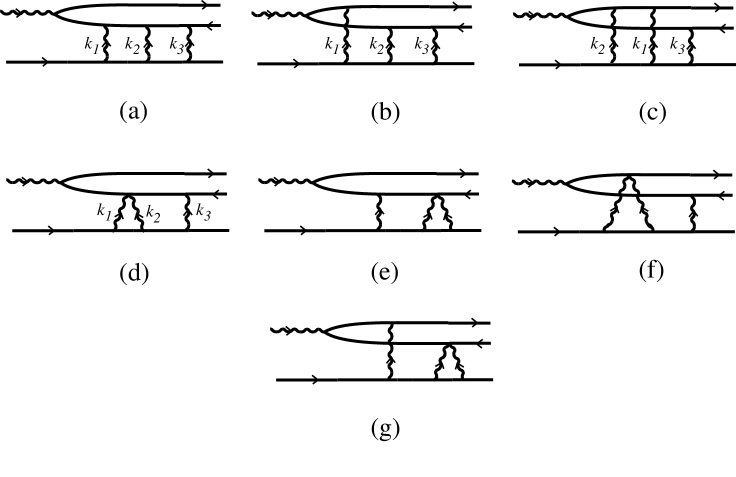
Figure 8: Diagrams that can contribute to the two-loop amplitude $C$ in $A^{+}=0$ gauge. All permutations of the attachments to the target line are implied.

Here we evaluate the three-gluon exchange amplitude $C$ (37) in $A^{+}=0$ gauge and in the kinematic limit (53). The leading order diagrams $C_{a}\ldots C_{g}$ are displayed in Fig. 8. For each diagram, the $6$ permutations of the vertices on the target line are taken into account. Since two permutations correspond to the same topology for diagrams $C_{d}\ldots C_{g}$, there is a factor $1/2$ for those diagrams. We will use the following shorthand notations:

$$\int_{\perp}\equiv\int\frac{d^{2}\vec{k}_{1\perp}}{(2\pi)^{2}}\,\frac{d^{2}\vec{k}_{2\perp}}{(2\pi)^{2}}\,\frac{1}{k_{1\perp}^{2}k_{2\perp}^{2}k_{3\perp}^{2}}\ ;\ \int_{+}\equiv\int\frac{dk_{1}^{+}}{2\pi}\frac{dk_{2}^{+}}{2\pi}\ ;\ \int_{-}\equiv\int\frac{dk_{1}^{-}}{2\pi i}\frac{dk_{2}^{-}}{2\pi i}$$

$$J =\frac{1}{\left[k_{1}^{-}+k_{1\perp}^{2}/M-i\epsilon\right]\left[k_{1}^{-}+k_{2}^{-}+(\vec{k}_{1\perp}+\vec{k}_{2\perp})^{2}/M-i\epsilon\right]}+{\rm perm}\,(k_{1},k_{2},k_{3})$$

(where $J$ contains $6$ terms arising from the $6$ permutations mentioned above), and

$$D_{ij}\equiv D(\vec{p}_{i\perp}-\vec{k}_{j\perp})\ ;\ D_{i}\equiv D(\vec{p}_{i\perp})\ ;\ {\rm for}\ i=1,2\ {\rm and}\ j=1,2,3$$ (72)

where $D$ is defined in (21). Using the kinematic limit (53) and approximations as in (54) and (55), the scalar abelian Feynman rules give:

$$C_{a} = -2eg^{6}QM\int_{\perp}\int_{-}J\int_{+}\frac{N_{1}N_{2}N_{3}}{k_{1}^{+}k_{2}^{+}k_{3}^{+}}\frac{1}{-D_{1}(p_{2}^{-}k_{1}^{+}-D_{11}+i\epsilon)(-p_{2}^{-}k_{3}^{+}-N_{3}+i\epsilon)}$$

$$C_{b} = -2eg^{6}QM\int_{\perp}\int_{-}J\int_{+}\frac{N_{1}N_{2}N_{3}}{k_{1}^{+}k_{2}^{+}k_{3}^{+}}$$

$$\times \frac{1}{(-p_{1}^{-}k_{1}^{+}+N_{1}+i\epsilon)(p_{2}^{-}k_{1}^{+}-D_{11}+i\epsilon)(-p_{2}^{-}k_{3}^{+}-N_{3}+i\epsilon)}$$

$$C_{c} = -2eg^{6}QM\int_{\perp}\int_{-}J\int_{+}\frac{N_{1}N_{2}N_{3}}{k_{1}^{+}k_{2}^{+}k_{3}^{+}}$$

$$\times \frac{1}{(-p_{1}^{-}k_{1}^{+}+N_{1}+i\epsilon)(-p_{1}^{-}(k_{1}^{+}+k_{2}^{+})+N_{1}+N_{2}+i\epsilon)(-p_{2}^{-}k_{3}^{+}-N_{3}+i\epsilon)}$$

$$C_{d} = -2eg^{6}QM\int_{\perp}\int_{-}J\int_{+}\frac{N_{3}\,\vec{k}_{1\perp}\cdot\vec{k}_{2\perp}}{k_{1}^{+}k_{2}^{+}k_{3}^{+}}\frac{1}{-D_{1}(-p_{2}^{-}k_{3}^{+}-N_{3}+i\epsilon)}$$

$$C_{e} = -2eg^{6}QM\int_{\perp}\int_{-}J\int_{+}\frac{N_{1}\,\vec{k}_{2\perp}\cdot\vec{k}_{3\perp}}{k_{1}^{+}k_{2}^{+}k_{3}^{+}}\frac{1}{-D_{1}(p_{2}^{-}k_{1}^{+}-D_{11}+i\epsilon)}$$

$$C_{f} = -2eg^{6}QM\int_{\perp}\int_{-}J\int_{+}\frac{N_{3}\,\vec{k}_{1\perp}\cdot\vec{k}_{2\perp}}{k_{1}^{+}k_{2}^{+}k_{3}^{+}}$$

$$\times \frac{1}{(-p_{1}^{-}(k_{1}^{+}+k_{2}^{+})+N_{1}+N_{2}+i\epsilon)(-p_{2}^{-}k_{3}^{+}-N_{3}+i\epsilon)}$$

$$C_{g} = -2eg^{6}QM\int_{\perp}\int_{-}J\int_{+}\frac{N_{1}\,\vec{k}_{2\perp}\cdot\vec{k}_{3\perp}}{k_{1}^{+}k_{2}^{+}k_{3}^{+}}\frac{1}{(-p_{1}^{-}k_{1}^{+}+N_{1}+i\epsilon)(p_{2}^{-}k_{1}^{+}-D_{11}+i\epsilon)}$$

with

$$N_{1}=D_{1}-D_{11}\ ;\ N_{2}=D_{11}-D_{23}\ ;\ N_{3}=D_{23}-D_{2}$$ (74)

Similarly to what was done in Appendix A for the one-loop calculation, one now considers all integrands in (LABEL:Cdiag) as rational functions of $k_{i}^{+}$ ($i=1,2,3$), which we decompose in simple elements, making first use of

$$\frac{1}{k_{1}^{+}k_{2}^{+}k_{3}^{+}}=\frac{1}{k^{+}}\left(\frac{1}{k_{1}^{+}k_{2}^{+}}+\frac{1}{k_{1}^{+}k_{3}^{+}}+\frac{1}{k_{2}^{+}k_{3}^{+}}\right)$$ (75)

The limit $p_{1}^{-}\to\infty$ must be taken after the decomposition in simple elements has been completed, otherwise some pinch singularities can arise. As there are in the two-loop case two independent ‘$+$’ integration variables ($k_{1}^{+}+k_{2}^{+}+k_{3}^{+}=k^{+}$), each integrand can be expressed as a sum of terms having one of the following forms:

$$\frac{1}{k_{i}^{+}k_{j}^{+}}\ ;\ \frac{1}{k_{i}^{+}(k_{j}^{+}\pm i\epsilon)}\ ;\ \frac{1}{(k_{i}^{+}\pm i\epsilon)(k_{j}^{+}\pm i\epsilon)}\ \ \ (i\neq j)$$ (76)

In (76) the poles at $k_{i}^{+}=0$ come from the gluon propagators in LC $A^{+}=0$ gauge, whereas those at $k_{i}^{+}=\pm i\epsilon$ originate from the scalar quark propagators. The result of the full decomposition is

$$C_{a} = -2eg^{6}QMp_{2}^{-}\int_{\perp}\int_{-}J\int_{+}$$

$$\times \left\{\left(\frac{1}{D_{23}}-\frac{1}{D_{11}}\right)\left(1-\frac{D_{11}}{D_{1}}\right)\left(\frac{D_{23}}{D_{2}}-1\right)\left[\frac{1}{k_{1}^{+}+i\epsilon}-\frac{1}{k_{1}^{+}}\right]\left[\frac{1}{k_{2}^{+}}+\frac{1}{k_{3}^{+}-i\epsilon}\right]\right.$$

$$+ \left.\left(\frac{1}{D_{11}}-\frac{1}{D_{1}}\right)\frac{D_{11}-D_{23}}{D_{2}}\left[\frac{1}{k_{1}^{+}+i\epsilon}-\frac{1}{k_{1}^{+}}\right]\left[\frac{1}{k_{3}^{+}}-\frac{1}{k_{3}^{+}-i\epsilon}\right]\right.$$

$$+ \left.\frac{(D_{1}-D_{11})(D_{11}-D_{23})}{D_{1}D_{2}(D_{2}-D_{11})}\left[\frac{1}{k_{1}^{+}+i\epsilon}+\frac{1}{k_{2}^{+}}\right]\left[\frac{1}{k_{3}^{+}}-\frac{1}{k_{3}^{+}-i\epsilon}\right]\right\}$$

$$C_{b} = -2eg^{6}QMp_{2}^{-}\int_{\perp}\int_{-}J\int_{+}$$

$$\times \left\{\left(\frac{1}{D_{2}}-\frac{1}{D_{23}}\right)\left(1-\frac{D_{23}}{D_{11}}\right)\left[\frac{1}{k_{2}^{+}}+\frac{1}{k_{3}^{+}-i\epsilon}\right]\left[\frac{1}{k_{1}^{+}}-\frac{1}{k_{1}^{+}-i\epsilon}\right]\right.$$

$$+ \left.\frac{1}{D_{2}}\left(1-\frac{D_{23}}{D_{11}}\right)\left[\frac{1}{k_{3}^{+}}-\frac{1}{k_{3}^{+}-i\epsilon}\right]\left[\frac{1}{k_{1}^{+}}-\frac{1}{k_{1}^{+}-i\epsilon}\right]\right\}$$

$$C_{c} = -2eg^{6}QMp_{2}^{-}\int_{\perp}\int_{-}J\int_{+}$$

$$\times \left(\frac{1}{D_{23}}-\frac{1}{D_{2}}\right)\frac{D_{11}-D_{23}}{D_{1}-D_{23}}\left[\frac{1}{k_{2}^{+}}+\frac{1}{k_{3}^{+}+i\epsilon}\right]\left[\frac{1}{k_{1}^{+}}-\frac{1}{k_{1}^{+}-i\epsilon}\right]$$

$$C_{d} = -2eg^{6}QMp_{2}^{-}\int_{\perp}\int_{-}J\int_{+}\frac{\vec{k}_{1\perp}\cdot\vec{k}_{2\perp}}{D_{1}D_{2}}\left\{\left[\frac{1}{k_{1}^{+}}+\frac{1}{k_{2}^{+}}\right]\left[\frac{1}{k_{3}^{+}}-\frac{1}{k_{3}^{+}-i\epsilon}\right]\right.$$

$$+ \left.\left(1-\frac{D_{2}}{D_{23}}\right)\left[\frac{1}{k_{1}^{+}}-\frac{1}{k_{1}^{+}+i\epsilon}\right]\left[\frac{1}{k_{2}^{+}}+\frac{1}{k_{3}^{+}-i\epsilon}\right]\right\}$$

$$C_{e} = -2eg^{6}QMp_{2}^{-}\int_{\perp}\int_{-}J\int_{+}\frac{\vec{k}_{2\perp}\cdot\vec{k}_{3\perp}}{D_{1}D_{2}}\left\{\left(1-\frac{D_{1}}{D_{11}}\right)\left[\frac{1}{k_{2}^{+}}+\frac{1}{k_{3}^{+}}\right]\left[\frac{1}{k_{1}^{+}+i\epsilon}-\frac{1}{k_{1}^{+}}\right]\right.$$

$$+ \left.\frac{D_{11}-D_{1}}{D_{2}-D_{11}}\left[\frac{1}{k_{2}^{+}}-\frac{1}{k_{2}^{+}-i\epsilon}\right]\left[\frac{1}{k_{3}^{+}}+\frac{1}{k_{1}^{+}+i\epsilon}\right]\right\}$$

$$C_{f} = -2eg^{6}QMp_{2}^{-}\int_{\perp}\int_{-}J\int_{+}\frac{\vec{k}_{1\perp}\cdot\vec{k}_{2\perp}}{D_{1}-D_{23}}$$

$$\times \left(\frac{1}{D_{2}}-\frac{1}{D_{23}}\right)\left[\frac{1}{k_{1}^{+}-i\epsilon}-\frac{1}{k_{1}^{+}}\right]\left[\frac{1}{k_{2}^{+}}+\frac{1}{k_{3}^{+}+i\epsilon}\right]$$

$$C_{g} = -2eg^{6}QMp_{2}^{-}\int_{\perp}\int_{-}J\int_{+}\frac{-\vec{k}_{2\perp}\cdot\vec{k}_{3\perp}}{D_{2}D_{11}}\left[\frac{1}{k_{2}^{+}}+\frac{1}{k_{3}^{+}}\right]\left[\frac{1}{k_{1}^{+}}-\frac{1}{k_{1}^{+}-i\epsilon}\right]$$ (77)

Eq. (77) can be conveniently used to group together the poles at $k_{i}^{+}=0$, which appear in the two first forms of (76). For each of these forms, a lengthy calculation shows that the $k_{i}^{+}=0$ poles add to a contribution which is identically zero, analogously to (S0.Ex46) for the one-loop calculation. On the way we use the identities

$$-2\vec{k}_{1\perp}\cdot\vec{k}_{2\perp}=D_{11}+D_{12}-D_{23}-D_{1}$$

$$-2\vec{k}_{2\perp}\cdot\vec{k}_{3\perp}=D_{13}+D_{12}-D_{21}-D_{1}$$ (78)

$$D_{2}+D_{11}+D_{12}+D_{13}-D_{21}-D_{22}-D_{23}-D_{1}=0$$ (79)

and realize that in every factor $[1/k_{i}^{+}\pm 1/(k_{j}^{+}\pm i\epsilon)]$ ($i\neq j$) of (77), $k_{j}^{+}$ can be replaced by $k_{i}^{+}$ (and not the contrary) by a change of variable. We also use the symmetry of $\int_{\perp}$ and $J$ under $k_{i}\leftrightarrow k_{j}$ for $i\neq j$.

Thus we have explicitly checked the complete prescription independence of our two-loop calculation. Only terms of the last form of (76) remain in (77). Using

$$\int_{-}J(k_{1}^{-},k_{2}^{-})=1$$ (80)

as well as (S0.Ex84), (79) and symmetry arguments, one shows that these terms add to

$$C=-\frac{1}{3}eg^{6}MQp_{2}^{-}\int_{\perp}\left[\frac{1}{D_{2}}-\frac{3}{D_{23}}+\frac{3}{D_{11}}-\frac{1}{D_{1}}\right]$$ (81)

which exactly reproduces the result (37) obtained in Feynman gauge (for large $M$).

After having shown the complete prescription independence of our calculation, we conclude this Appendix with some important remarks. We stress that (LABEL:Cdiag) and (77) are equivalent mathematical expressions for any of the diagrams $C_{a}\ldots C_{g}$. To evaluate a given diagram, one needs to regularize the $k_{i}^{+}=0$ poles, but this can be done starting either from (LABEL:Cdiag) or from (77), and the same results must follow. We have checked this for all diagrams using the PV and K prescriptions. We thus see no problems in applying the PV prescription to two-loop diagrams. Using the PV prescription on (77) is straightforward, but applying it to (LABEL:Cdiag) requires some comments. Regularizing $1/(k_{1}^{+}k_{2}^{+}k_{3}^{+})$ yields

$$\frac{1}{k_{1}^{+}k_{2}^{+}k_{3}^{+}}\rightarrow\prod_{i=1}^{3}{\rm PV}\left(\frac{1}{k_{i}^{+}}\right)=\lim_{\eta_{3}\to 0}\lim_{\eta_{2}\to 0}\lim_{\eta_{1}\to 0}\left[\frac{1}{k_{1}^{+}}\right]_{\eta_{1}}\left[\frac{1}{k_{2}^{+}}\right]_{\eta_{2}}\left[\frac{1}{k_{3}^{+}}\right]_{\eta_{3}}$$ (82)

where $[1/k_{i}^{+}]_{\eta_{i}}$ is given in (64). Thus the poles at $k_{i}^{+}=0$ must be regularized with distinct small finite parameters $\eta_{i}$. Then the $k_{i}^{+}$ integrals are performed using Cauchy’s theorem, and only in the end the limits $\eta_{1}\to 0$, $\eta_{2}\to 0$, $\eta_{3}\to 0$ are taken separately (in arbitrary order). We found this procedure to be well-defined and to give results consistent with those directly obtained from (77).

Finally, as in the one-loop case, it is remarkable that the K prescription makes all two-loop diagrams where the fast quark rescatters vanish, i.e., only $C_{a}$, $C_{d}$ and $C_{e}$ contribute to the amplitude $C$.

C. Absence of struck quark rescattering in $A^{+}=0$ gauge.

In this Appendix we show that in $A^{+}=0$ gauge, independently of the prescription used to regularize the spurious $k_{i}^{+}=0$ poles, rescatterings of the struck quark $p_{1}$ cancel in the cross section, i.e.  after summing over cuts in the forward Compton amplitude. This is done by proving that the full contribution to the cross section (use Eqs. (27), (36), (38))

$$\int d^{2}\vec{r}_{\perp}\,d^{2}\vec{R}_{\perp}\,\left[|{\tilde{B}}|^{2}+2{\tilde{A}}{\tilde{C}}\right]=-\frac{1}{3}(eg^{4}QMp_{2}^{-})^{2}\int d^{2}\vec{r}_{\perp}\,d^{2}\vec{R}_{\perp}\,V(m_{||}r_{\perp})^{2}W(\vec{r}_{\perp},\vec{R}_{\perp})^{4}$$ (83)

is given by attachments to $p_{2}$ only.

We need to know the partial amplitudes $A_{2}$, $B_{2}$, $C_{2}$ contributing to $A$, $B$, $C$ where only attachments to $p_{2}$ are kept. For the Born amplitude $A$, only the diagram of Fig. 4a contributes in $A^{+}=0$ gauge. Thus the partial amplitude $A_{2}$ from attachments to $p_{2}$ is actually the full amplitude $A$ given in (22),

$$A_{2}=A=\frac{2eg^{2}MQp_{2}^{-}}{k_{\perp}^{2}}\left[\frac{1}{D_{2}}-\frac{1}{D_{1}}\right]$$ (84)

The partial one-loop amplitude $B_{2}$ is given by the sum of the diagrams $B_{a}$, $B_{b}$ and $B_{e}$ of Fig. 7. This sum is prescription dependent. We use the notation (see Eq. (64))

$$I_{\eta}=\int\frac{dk_{2}^{+}}{i\pi}\left[\frac{1}{k_{2}^{+}}\right]_{\eta}$$ (85)

giving $I_{PV}=0$ and $I_{K}=1$. After regularizing (60) and using (62) and symmetry arguments we find,

$$B_{2}=B_{a}+B_{b}+B_{e}=-i\,eg^{4}QMp_{2}^{-}\int_{\perp}\left[\left(\frac{1}{D_{1}}-\frac{1}{D_{22}}\right)+I_{\eta}\,\left(\frac{1}{D_{2}}-\frac{1}{D_{22}}\right)\right]$$ (86)

The partial two-loop amplitude $C_{2}$ is given by the diagrams $C_{a}$, $C_{d}$ and $C_{e}$ of Fig. 8. Regularizing (77) and using (80) we get

$$C_{a} = -\frac{1}{2}eg^{6}QMp_{2}^{-}\int_{\perp}\,\left\{\left(\frac{1}{D_{23}}-\frac{1}{D_{11}}\right)\left(1-\frac{D_{11}}{D_{1}}\right)\left(\frac{D_{23}}{D_{2}}-1\right)(I_{\eta}+1)^{2}\right.$$

$$+ \left.\left(\frac{1}{D_{11}}-\frac{1}{D_{1}}\right)\frac{D_{11}-D_{23}}{D_{2}}(I_{\eta}^{2}-1)-\frac{(D_{1}-D_{11})(D_{11}-D_{23})}{D_{1}D_{2}(D_{2}-D_{11})}(I_{\eta}-1)^{2}\right\}$$

$$C_{d} = \frac{1}{2}eg^{6}QMp_{2}^{-}\int_{\perp}\frac{\vec{k}_{1\perp}\cdot\vec{k}_{2\perp}}{D_{1}D_{2}}\left\{2I_{\eta}(I_{\eta}-1)+\left(1-\frac{D_{2}}{D_{23}}\right)(I_{\eta}+1)^{2}\right\}$$

$$C_{e} = \frac{1}{2}eg^{6}QMp_{2}^{-}\int_{\perp}\frac{\vec{k}_{2\perp}\cdot\vec{k}_{3\perp}}{D_{1}D_{2}}\left\{\left(1-\frac{D_{1}}{D_{11}}\right)2I_{\eta}(-I_{\eta}-1)+\frac{D_{11}-D_{1}}{D_{2}-D_{11}}(I_{\eta}-1)^{2}\right\}$$

Using (S0.Ex84), (79) and symmetry arguments we get after some algebra

$$C_{2} = C_{a}+C_{d}+C_{e}=-\frac{1}{2}eg^{6}QMp_{2}^{-}\int_{\perp}$$

$$\left\{\left[-\frac{2}{3D_{1}}+\frac{1}{6D_{2}}-\frac{1}{2D_{23}}+\frac{1}{D_{11}}\right]+I_{\eta}\left[-\frac{1}{D_{23}}+\frac{1}{D_{11}}\right]+I_{\eta}^{2}\left[\frac{1}{2D_{2}}-\frac{1}{2D_{23}}\right]\right\}$$

It is an easy exercise to express the partial amplitudes $A_{2}$, $B_{2}$, $C_{2}$ in transverse coordinate space, as was done for the full amplitudes $A$, $B$, $C$ in section 5 (see Eq. (24)). Since the partial amplitudes are not infrared finite, we introduce a small photon mass $\lambda$ in the exchanged photon propagators, i.e.  $1/k_{i\perp}^{2}\rightarrow 1/(k_{i\perp}^{2}+\lambda^{2})$ in the definition of $\int_{\perp}$ (S0.Ex38) or (S0.Ex58). Then

$${\tilde{A}_{2}} = \ 2\,eg^{2}QMp_{2}^{-}VW$$

$${\tilde{B}_{2}} = -i\,eg^{4}QMp_{2}^{-}VW\,\frac{I_{\eta}K_{0}(\lambda R_{\perp})-K_{0}(\lambda|\vec{R}_{\perp}+\vec{r}_{\perp}|)}{2\pi}$$

$${\tilde{C}_{2}} = -\frac{1}{4}\,eg^{6}QMp_{2}^{-}VW\left[\frac{W^{2}}{3}+\left(\frac{I_{\eta}K_{0}(\lambda R_{\perp})-K_{0}(\lambda|\vec{R}_{\perp}+\vec{r}_{\perp}|)}{2\pi}\right)^{2}\right]$$ (89)

where $V$ and $W$ stand for $V(m_{||}r_{\perp})$ and $W(\vec{r}_{\perp},\vec{R}_{\perp})$. The contribution from attachments to $p_{2}$ to the cross section reads

$$\int d^{2}\vec{r}_{\perp}\,d^{2}\vec{R}_{\perp}\,\left[|{\tilde{B}_{2}}|^{2}+2{\tilde{A}_{2}}{\tilde{C}_{2}}\right]=-\frac{1}{3}(eg^{4}QMp_{2}^{-})^{2}\int d^{2}\vec{r}_{\perp}\,d^{2}\vec{R}_{\perp}\,V^{2}W^{4}$$ (90)

This is infrared finite, prescription independent, and identical to the full result (83). Hence rescatterings of the struck quark $p_{1}$ cancel in the cross section in $A^{+}=0$ gauge.

From (83) and (90) we see that in $A^{+}=0$ gauge and in coordinate space, the contribution from attachments to $p_{2}$ equals the full contribution $|B|^{2}+2AC$ even at the integrand level, i.e.  before integrating over $\vec{r}_{\perp}$ and $\vec{R}_{\perp}$. We thus have, in coordinate space,

$$|{\tilde{\cal M}}|^{2}=|{\tilde{\cal M}_{2}}|^{2}$$ (91)

where ${\tilde{\cal M}}=\tilde{A}+\tilde{B}+\tilde{C}+\ldots$ is given in (39) and ${\tilde{\cal M}_{2}}=\tilde{A}_{2}+\tilde{B}_{2}+\tilde{C}_{2}+\ldots$ corresponds to the partial amplitude where only attachments to $p_{2}$ are kept. Thus in $A^{+}=0$ gauge

$${\tilde{\cal M}}(\vec{r}_{\perp},\vec{R}_{\perp})=e^{i\phi}{\tilde{\cal M}_{2}}(\vec{r}_{\perp},\vec{R}_{\perp})$$ (92)

The full amplitude ${\tilde{\cal M}}$ is obtained from ${\tilde{\cal M}_{2}}$ by inserting any number of rescatterings of the quark $p_{1}$. Eq. (92) reads

$$\tilde{A}+\tilde{B}+\tilde{C}+\ldots=e^{i\phi}\,(\tilde{A}_{2}+\tilde{B}_{2}+\tilde{C}_{2}+\ldots)$$ (93)

By expanding the l.h.s. and r.h.s. of (93) up to order $g^{6}$, one realizes that $\phi$ must be at least of order $g^{2}$,

$$\phi=\phi_{1}\,g^{2}+\phi_{2}\,g^{4}+\ldots$$ (94)

Identification of the terms of order $g^{4}$ and $g^{6}$ in the two sides of (93) leads to

$$\phi_{1} = \frac{I_{\eta}-1}{4\pi}\,K_{0}(\lambda R_{\perp})$$

$$\phi_{2} = 0$$ (95)

or

$$\phi=g^{2}\,\frac{I_{\eta}-1}{4\pi}\,K_{0}(\lambda R_{\perp})+{\cal{O}}(g^{6})$$ (96)

Although not proven here, the ${\cal O}\left(g^{6}\right)$ terms in $\phi$ are expected to vanish because adding one rescattering of $p_{1}$ can only bring a power $g^{2}$ (see also the following discussion). Thus we get

$${\tilde{\cal M}}(\vec{r}_{\perp},\vec{R}_{\perp})={\rm exp}{\left[i\frac{g^{2}}{4\pi}(I_{\eta}-1)K_{0}(\lambda R_{\perp})\right]}\,{\tilde{\cal M}_{2}}(\vec{r}_{\perp},\vec{R}_{\perp})$$ (97)

As expected, since ${\tilde{\cal M}}$ is infrared safe and prescription independent, all the dependence on $\lambda$ and $I_{\eta}$ of ${\tilde{\cal M}_{2}}$ is contained in the phase. Note also that with the K prescription, $I_{\eta}=1$ and ${\tilde{\cal M}}={\tilde{\cal M}_{2}}$.

Eq. (97) can also be understood as follows. In momentum space, if we call $\mu$ the Lorentz index associated to the coupling of $p_{1}$, we know that the amplitude is dominated by the $n^{\nu}k_{i}^{\mu}/k_{i}^{+}$ term of the exchanged gluon propagator in $A^{+}=0$ gauge, with $\mu=\perp$ and $\nu=-$. Together with the scalar quark propagator

$$\Delta_{i}^{-1}\propto(p_{1}-k_{i})^{2}-m^{2}+i\varepsilon\simeq-p_{1}^{-}k_{i}^{+}+a_{i}+i\varepsilon$$ (98)

where $a_{i}=D(p_{1})-D(p_{1}-k_{i})$, the factor $1/k_{i}^{+}$ yields

$$\int\frac{dk_{i}^{+}}{2\pi i}\frac{1}{(-p_{1}^{-}k_{i}^{+}+a_{i}+i\varepsilon)k_{i}^{+}}\rightarrow\frac{1}{a_{i}}\int\frac{dk_{i}^{+}}{2\pi i}\left(\left[\frac{1}{k_{i}^{+}}\right]_{\eta}+\frac{1}{-k_{i}^{+}+i\varepsilon}\right)=\frac{1}{a_{i}}\frac{I_{\eta}-1}{2}$$ (99)

where some simplification similar to (58) was made. The scalar coupling brings a factor $g^{2}\vec{k}_{i\perp}\cdot(2\vec{p}_{1}-\vec{k}_{i})_{\perp}=g^{2}a_{i}$ which compensates the prefactor in the r.h.s of (99). We are left with the $1/(k_{i\perp}^{2}+\lambda^{2})$ factor from the gluon propagator, which after Fourier transform gives $K_{0}(\lambda R_{\perp})/(2\pi)$. This builds the complete phase in (97).

References

[1]
S. D. Drell and T.-M. Yan, Phys. Rev. Lett. 24, 181 (1970);
S. D. Drell, D. J. Levy and T.-M. Yan, Phys. Rev. D1, 1035 (1970).
[2]
V. N. Gribov,
Sov. Phys. JETP 29, 483 (1969) [Zh. Eksp. Teor. Fiz. 56, 892 (1969)].
[3]
S. J. Brodsky and J. Pumplin,
Phys. Rev. 182, 1794 (1969).
[4]
S. J. Brodsky and H. J. Lu,
Phys. Rev. Lett. 64, 1342 (1990).
[5]
G. Piller and W. Weise,
Phys. Rept. 330, 1 (2000) [hep-ph/9908230].
[6]
S. J. Brodsky, D. S. Hwang and I. Schmidt,
hep-ph/0201296.
[7]
S. J. Brodsky, M. Diehl and D. S. Hwang, Nucl. Phys. B596, 99 (2001)
[hep-ph/0009254];
M. Diehl, T. Feldmann, R. Jakob and P. Kroll, Nucl. Phys. B596, 33 (2001)
[hep-ph/0009255].
[8]
J. C. Collins and D. E. Soper, Nucl. Phys. B194, 445 (1982);
J. C. Collins, D. E. Soper and G. Sterman, Nucl. Phys. B261, 104 (1985),
Nucl. Phys. B308, 833 (1988), Phys. Lett. B438, 184 (1998) and review in Perturbative
Quantum Chromodynamics, (A.H. Mueller, ed.,World Scientific Publ., 1989, pp.
1-91);
G. T. Bodwin, Phys. Rev. D31, 2616 (1985), Erratum Phys. Rev. D34, 3932 (1986).
[9]
V. N. Gribov, Sov. Phys. JETP 29, 483 (1969) and 30, 709 (1970).
[10]
G. Piller and W. Weise, Phys. Rep. 330, 1 (2000) [hep-ph/9908230];
G. Piller, M. Vänttinen, L. Mankiewicz and W.
Weise, [hep-ph/0010037];
L. Frankfurt, V. Guzey, M. McDermott and M. Strikman,
[hep-ph/0201230].
[11]
G. P. Lepage and S. J. Brodsky, Phys. Rev. D22, 2157 (1980).
[12]
J. D. Bjorken, J. B. Kogut and D. E. Soper, Phys. Rev. D3, 1382 (1971).
[13]
S. J. Brodsky, P. Hoyer and L. Magnea, Phys. Rev. D55, 5585 (1997) [hep-ph/9611278].
[14] S. Klein, Rev. Mod. Phys. 71, 1501 (1999).
[15] H. A. Bethe and L. C. Maximon, Phys. Rev. 93,768
(1954); H. Davies, H. A. Bethe and L. C. Maximon, ibid.,93, 788
(1954).
[16] G. Leibbrandt, Rev. Mod. Phys. 59, 1067 (1987).
[17] Y. V. Kovchegov, Phys. Rev. D55, 5445 (1997) [hep-ph/9701229].
[18]
P. V. Landshoff, J. C. Polkinghorne and R. D. Short,
Nucl. Phys. B 28, 225 (1971).
[19]
S. J. Brodsky, F. E. Close and J. F. Gunion,
Phys. Rev. D 8, 3678 (1973).