DFPD-01/TH/12

Double chiral logarithms of Generalized Chiral Perturbation Theory for low-energy $\pi\pi$ scattering

Luca Girlanda

Dipartimento di Fisica “Galileo Galilei”, Università di Padova and INFN
Via Marzolo 8, I-35131 Padova, Italy

We express the two-massless-flavor Gell-Mann–Oakes–Renner ratio in terms of low-energy $\pi\pi$ observables including the $O(p^{6})$ double chiral logarithms of generalized chiral perturbation theory. Their contribution is sizeable and tends to compensate the one from the single chiral logarithms. However it is not large enough to spoil the convergence of the chiral expansion. As a signal of reduced theoretical uncertainty, we find that the scale dependence from the one-loop single logarithms is almost completely canceled by the one from the two-loop double logarithms.

Keywords: Chiral symmetry, Dynamical symmetry breaking, Quark condensate, Chiral perturbation theory, Renormalization group equations, $\pi\pi$ scattering.

PACS: 11.30.Rd, 12.39.Fe, 11.10.Hi, 13.75.Lb

1.  The dynamics of chiral symmetry breakdown ($\chi$SB) in the Standard Model remains an open issue both from the experimental and theoretical standpoint. At very low energy the problem concerns the understanding of the mechanism of $\chi$SB for QCD. In this framework it is generally assumed that chiral symmetry is broken through the formation of a quark-antiquark condensate. A theoretically consistent alternative is that the symmetry is broken by higher dimensional order parameters, analogously to what happens in antiferromagnetic spin systems for the rotational symmetry [1]. Deeper insight into this problem can be gained by considering the theory in a Euclidean box, with (anti)periodic boundary conditions. The two alternatives are then distinguished by a qualitatively different behavior of the smallest eigenvalues of the Dirac operator in the thermodynamical limit. In fact it has recently been realized that a prominent role is played by the number of massless flavors $N_{f}$ of the theory [2, 3]. In general, as $N_{f}$ increases, the order parameters dominated by the infrared end of the spectrum of the Euclidean Dirac operator experience a paramagnetic suppression which, for $N_{f}$ large enough, will eventually restore chiral symmetry. Since only the SU(2) and SU(3) chiral limits are reasonable approximations to the real world, the question to be addressed is to which extent $N_{f}=2,3$ is close to a critical point in which $\langle\bar{q}q\rangle$ disappears and chiral symmetry is eventually broken by higher-dimensional order parameters. As was pointed out in Refs. [4, 5], it is possible to submit the standard hypothesis of a large condensate to experimental verification, through the measurement of low-energy $\pi\pi$ phase-shifts. The S-wave $\pi\pi$ interaction at low energy is very sensitive to the two-massless-flavor chiral condensate: it gets stronger as the condensate decreases. Standard chiral perturbation theory (ChPT) [6] pushed to two-loop accuracy, together with the use of constraints from Roy equations [7], provides a very sharp prediction for the S-wave scattering lengths [8]. The situation has evolved recently, since new preliminary experimental data provided by the E865 experiment on $K_{e4}$ decays have become available [9]. In fact a first analysis of the above mentioned data in the standard context indicates that deviations from this scenario are marginal [10]. On the other hand, generalized chiral perturbation theory (GChPT), which relaxes from the beginning the standard assumption, cannot produce any prediction for the low-energy $\pi\pi$ observables, but only relates these observables to the magnitude of the quark condensate. It is the purpose of the present work to establish the relationship between low-energy $\pi\pi$ observables and the two-massless-flavors quark condensate in the language of GChPT beyond the $O(p^{4})$ level, i.e. including the $O(p^{6})$ double chiral logarithms, which are among the potentially most dangerous two-loop contributions.

2.  Relaxing the standard assumption of a dominant condensate implies that the Gell-Mann–Oakes–Renner ratio,

$$x_{2}^{\mathrm{GOR}}=\frac{(m_{u}+m_{d})}{F_{\pi}^{2}M_{\pi}^{2}}\lim_{m_{u},m_{d}\to 0}|\langle\bar{q}q\rangle|,$$ (1)

is actually a free parameter. If its value were not close to 1, then the quadratic term in quark masses would be as important as the condensate term in the chiral expansion of the squared pion mass. Thus the counting rule has to be modified accordingly: both the light quark mass $\hat{m}$ ($m_{u}=m_{d}=\hat{m}$) and the quark condensate are quantities of chiral order $O(p)$. The effective Lagrangian is organized as an infinite sum ${\mathcal{L}}={\mathcal{L}}^{(2)}+{\mathcal{L}}^{(3)}+{\mathcal{L}}^{(4)}+\ldots$ where the $O(p^{d})$ term ${\mathcal{L}}^{(d)}$ contains terms with $k$ derivatives, $l$ powers of quark masses and $n$ powers of the quark condensate, such that $k+l+n=d$. It contains, at each finite chiral order, additional operators with respect to the corresponding standard Lagrangian. For instance, the leading $O(p^{2})$ Lagrangian reads,

$${\mathcal{L}}^{(2)} = \frac{F^{2}}{4}\left\{\langle D_{\mu}U^{\dagger}D^{\mu}U\rangle+2B\langle U^{\dagger}\chi+\chi^{\dagger}U\rangle+A\langle\left(U^{\dagger}\chi\right)^{2}+\left(\chi^{\dagger}U\right)^{2}\rangle\right.$$ (2)

$$\left.+Z^{P}\langle U^{\dagger}\chi-\chi^{\dagger}U\rangle^{2}+h_{0}\langle\chi^{\dagger}\chi\rangle+h_{0}^{\prime}\left(\det\chi+\det\chi^{\dagger}\right)\right\},$$

where $U\in$ SU(2) collects the Goldstone bosons’ degrees of freedom and $\chi$ denotes the scalar-pseudoscalar external source, to be expanded around the quark mass matrix $\chi=\hat{m}{\bf 1}+\ldots$. Notice that, compared to standard notations, a factor $2B$ has been removed from the definition of $\chi$, for consistency with the new chiral counting: in fact $B$ is related to the quark condensate, $F^{2}B=-\lim_{\hat{m}\to 0}\langle\bar{q}q\rangle$, and it has to be considered, formally, as a small parameter, $B\sim\chi\sim O(p)$. One-loop diagram with insertions from the Lagrangian (2) are of chiral order $O(p^{4})$. They are divergent and require the renormalization of the low-energy constants (l.e.c.). In the minimal subtraction scheme of dimensional regularization,

$${\mathrm{const}}={\mathrm{const}}^{r}+\frac{\mu^{d-4}}{16\pi^{2}}\frac{\Gamma_{\mathrm{const}}}{d-4},$$ (3)

where $\mu$ is the renormalization scale. The $\beta$-function coefficients $\Gamma_{\mathrm{const}}$ for the leading l.e.c.’s are

$$F^{2}\Gamma_{A}=3B^{2},\quad F^{2}\Gamma_{Z^{P}}=-\frac{3}{2}B^{2},\quad F^{2}\Gamma_{h_{0}^{\prime}}=6B^{2},$$ (4)

whereas $F^{2}$, $B$ and $h_{0}$ do not get renormalized. The renormalized constants are renormalization scale dependent, according to

$$\mu\frac{d}{d\mu}{\mathrm{const}}^{r}=-\frac{1}{16\pi^{2}}\Gamma_{\mathrm{const}}.$$ (5)

Due to the chiral counting of the condensate parameter $B$, the divergences arising from the renormalization of the l.e.c.’s are of chiral order $p^{4}$, as they should, in order to absorb the ones arising from the loops. The renormalization of the leading l.e.c.’s (4) is not sufficient to absorb all the one-loop $O(p^{4})$ divergences generated by ${\mathcal{L}}^{(2)}$, which is a consequence of the fact that the Lagrangian (2) is non-renormalizable. One has to include also the subleading $O(p^{3})$ and $O(p^{4})$ Lagrangians and renormalize the relative l.e.c.’s, according to Eq. (3). The $\beta$-function coefficients $\Gamma_{{\mathcal{L}}^{(3)}}$ for the l.e.c.’s of ${\mathcal{L}}^{(3)}$ will be proportional to $B$, in order that the divergences be of order $p^{4}$, while those for the l.e.c.’s of ${\mathcal{L}}^{(4)}$ will be independent of $B$,

$$\Gamma_{{\mathcal{L}}^{(2)}}\sim O(B^{2})\sim O(p^{2}),\quad\Gamma_{{\mathcal{L}}^{(3)}}\sim O(B)\sim O(p),\quad\Gamma_{{\mathcal{L}}^{(4)}}\sim O(1).$$ (6)

We refer to existing literature for the complete list of operators together with their renormalization up to $O(p^{4})$ [11].

3.  The proliferation of chirally invariant operators has no bearing on the form of the $\pi\pi$ scattering amplitude up to two-loop level: the latter only depends on six “observable” parameters, independently of the chiral counting. This is a consequence of unitarity, analyticity and crossing symmetry, and of the chiral suppression of partial waves greater than two [4]. Neglecting $O(p^{8})$, i.e. at two-loop level, the invariant amplitude for $\pi\pi$ scattering has been given, using dispersive methods, in Ref. [12] in terms of the parameters $\alpha,\beta,\lambda_{1},\ldots,\lambda_{4}$,

$$A(s|t,u)=A_{\mathrm{KMSF}}(s|t,u;\alpha,\beta;\lambda_{1},\lambda_{2},\lambda_{3},\lambda_{4})+O(p^{8}).$$ (7)

The parameter $\alpha$ represents, at leading order, the amplitude at the symmetric point $s=t=u=4/3M_{\pi}^{2}$, and $\beta$ its slope. These two parameters can be viewed as the subtraction constants in a Roy-like dispersive representation of the amplitude which fixes, confronted to existing experimental data in the medium and high energy region, the remaining 4 parameters $\lambda_{1},\ldots,\lambda_{4}$ [13]. A brute force calculation in ChPT allows one to find the “chiral anatomy” of these parameters, i.e.  their expressions in terms of quark masses and l.e.c.’s. In particular we are interested in finding their dependence on the l.e.c. $B$, related to the quark condensate. At tree level only the parameter $\alpha$ depends on the condensate: its value varies from 1 to 4 if $\langle\bar{q}q\rangle$ decreases from its standard value down to zero, while $\beta$ is equal to 1 and the $\lambda_{i}$’s vanish. Going to one-loop precision already involves a conspicuous set of l.e.c. characteristics of GChPT, besides the contribution of the chiral logarithms. Explicit expressions for the 1-loop parameters $\alpha$, $\beta$, $\lambda_{1}$ and $\lambda_{2}$ can be found in Refs. [11]. After eliminating as many unknown constants as possible in favor of physical quantities, one can invert these expressions for the quark condensate, and write the GOR ratio in terms of the combination $\alpha+2\beta$, modulo remaining unknown constants, renormalized at a scale $\mu$ [14]:

$$x_{2}^{\mathrm{GOR}} = \frac{2\hat{m}BF^{2}}{F_{\pi}^{2}M_{\pi}^{2}}=2-\frac{\alpha+2\beta}{3}+\frac{F^{2}}{F_{\pi}^{2}M_{\pi}^{2}}\left(15\rho_{1}^{r}-\rho_{2}^{r}+28\rho_{4}^{r}-2\rho_{5}^{r}\right)\hat{m}^{3}$$ (8)

$$+\left[4a_{2}^{r}+8\left(\frac{\alpha+2\beta}{3}-1\right)a_{3}+8b_{2}^{r}+16c_{1}^{r}\right]\hat{m}^{2}$$

$$+\frac{64}{M_{\pi}^{2}}(e_{1}^{r}+2f_{1}^{r}+2f_{2}^{r}+4f_{4}^{r})\hat{m}^{4}$$

$$+\frac{M_{\pi}^{2}}{288\pi^{2}F_{\pi}^{2}}\left(\alpha+2\beta\right)\left[24-11(\alpha+2\beta)\right]$$

$$+\left[6+\frac{5}{3}(\alpha+2\beta)-\frac{11}{9}(\alpha+2\beta)^{2}\right]\frac{M_{\pi}^{2}}{32\pi^{2}F_{\pi}^{2}}\log\frac{M_{\pi}^{2}}{\mu^{2}}\,.$$

The role of $\alpha$ and $\beta$ in this equation is that of observable quantities to be extracted from the data by fitting the two-loop formula (7), with the $\lambda_{i}$ fixed by the Roy equations. The standard prediction for $\alpha$ and $\beta$ is very close to 1 [15]. On the other hand the contribution from the l.e.c.’s figuring in Eq. (8) is unknown, at present. The $\rho_{i}$’s come from the $O(p^{3})$ ${\mathcal{L}}_{(0,3)}$ Lagrangian, with no derivatives and three powers of the scalar-pseudoscalar source, the constants $a_{i}$, $b_{i}$ and $c_{i}$ come from the $O(p^{4})$ ${\mathcal{L}}_{(2,2)}$ Lagrangian and the constants $e_{i}$, $f_{i}$ from the $O(p^{4})$ ${\mathcal{L}}_{(0,4)}$ Lagrangian, with analogous notations. In principle these l.e.c.’s should be determined from independent phenomenological information but, due to the large number of independent operators, this program seems hopeless. However we do know the scale dependence of all these l.e.c.’s. One possibility is thus to treat them as randomly distributed around zero with an error assigned to them according to naive dimensional analysis estimates,

$$\rho_{i}\sim\pm\frac{1}{\Lambda_{\mathrm{H}}},\quad a_{i},b_{i},c_{i},e_{i},f_{i}\sim\pm\frac{1}{\Lambda_{\mathrm{H}}^{2}},$$ (9)

where the hadronic scale $\Lambda_{\mathrm{H}}$ will be fixed to 1 GeV. The light quark mass $\hat{m}$ is written as $\hat{m}=m_{s}/r$, where the quark mass ratio $r$ is strongly correlated to the two-flavor GOR ratio (see e.g. Fig. 1 of Ref. [3]) and $m_{s}$ is taken conservatively to be $\sim 200$ MeV. As a consequence of the smallness of the light quark mass, these contributions will in practice be very small. On the contrary, the logarithmic terms in Eq. (8) will be quite important, specially in the region where $\alpha+2\beta$ is large. A further source of uncertainty is therefore the scale $\mu$ inside the logarithm, i.e. the scale at which the estimates (9) are supposed to hold. We will take $\mu=M_{\eta}\pm$250 MeV. The resulting curve is shown as the dashed line in Fig. 1, the band representing the theoretical uncertainty obtained as explained above. The main contribution to the error band is represented by the scale variation inside the logarithm. Due to the large contribution of the latter it becomes necessary to test the convergence of the chiral series, by studying the importance of higher orders. In the following we will compute the $O(p^{6})$ double logarithmic corrections to this result.

4.  Double chiral logarithms are among the potentially most dangerous contributions at order $O(p^{6})$ [16], because of the smallness of the pion mass. As first pointed out in Ref. [17] (see also Ref. [18]) they can be obtained from a 1-loop calculation, using the fact that, in the renormalization procedure, non-local divergences must cancel. We set the space-time dimension $d=4+\omega$ to regulate the theory. The coupling constant $F^{2}$, which multiplies the kinetic term for the pions, has dimension $[F^{2}]=d-2$. This constant appears as a common factor in the definition of the generalized chiral Lagrangian. Therefore, a generic l.e.c., with $k$ derivatives and $l$ powers of the scalar-pseudoscalar source, $c_{(k,l)}$, has mass dimension $2-k-l$, and does not depend on $\omega$. We thus replace $F^{2}$ with $\mu^{\omega}F^{2}$, making appear explicitly the scale parameter $\mu$ brought in by the regularization procedure. Since each loop involves a factor $F^{-2}$, the chiral expansion of a generic amplitude ${\mathcal{A}}$ up to two loops, apart from an overall dimensional factor, takes the form,

$${\mathcal{A}}\sim{\mathcal{A}}_{\mathrm{tree}}+\left(\frac{M_{\pi}}{\mu}\right)^{\omega}\sum_{i}P^{(1)}_{i}(c_{a})g_{i}^{\mathrm{1-loop}}+\left(\frac{M_{\pi}}{\mu}\right)^{2\omega}\sum_{i}P^{(2)}_{i}(c_{a})f_{i}^{\mathrm{2-loop}},$$ (10)

where $P_{i}^{(1,2)}$ are polynomials in the quark mass and l.e.c.’s, generically denoted by $c_{a}$, and $g_{i}$ and $f_{i}$ are loop-functions of the kinematical variables, expressed in terms of dimensionless quantities with the appropriate inverse powers of $M_{\pi}$. The loop functions are singular as $\omega\to 0$,

$$f_{i}=\frac{f_{i,2}}{\omega^{2}}+\frac{f_{i,1}}{\omega}+f_{i,0}+O(\omega),\quad g_{i}=\frac{g_{i,1}}{\omega}+g_{i,0}+O(\omega).$$ (11)

While the one-loop divergences are canceled by the renormalization of the l.e.c.’s of ${\mathcal{L}}^{(2)}+{\mathcal{L}}^{(3)}+{\mathcal{L}}^{(4)}$, appearing in ${\mathcal{A}}_{\mathrm{tree}}$,

$$c_{a}=\frac{\delta_{a}}{\omega}+c_{a}^{r}+O(\omega),$$ (12)

the two-loop divergences require the introduction of higher order local counterterms. We have defined, compared to the notations of Eq. (3),

$$\delta_{a}=\mu^{\omega}\frac{\Gamma_{a}}{16\pi^{2}},$$ (13)

which is actually independent of $\omega$, due to the fact that the $\beta$-function coefficients $\Gamma_{a}$ are all proportional to $F^{-2}$ (cfr. Eq. (4) and Ref. [11] for the ${\mathcal{L}}^{(3)}$ and ${\mathcal{L}}^{(4)}$ l.e.c.’s). Notice also that the divergent term in Eq. (12) always arises at chiral order $p^{4}$ in the generalized counting, as already mentioned, even if the constant itself is of lower order. Therefore, since the 1-loop polynomials $P_{i}^{(1)}$ are already of order $p^{4}$, we never have to deal, up to and including order $p^{6}$, with products of the type $\delta_{i}\delta_{j}g^{\mathrm{1-loop}}$: the polynomials $P_{i}^{(1)}$ after the substitution (12), can be rewritten as

$$P_{i}^{(1)}(c_{a})=P_{i}^{(1)}(c_{a}^{r})+\frac{\partial P_{i}^{(1)}}{\partial c_{b}}(c_{a}^{r})\frac{\delta_{b}}{\omega}.$$ (14)

For the same reason, since the 2-loop functions are of order $p^{6}$, the l.e.c.’s inside the polynomials $P_{i}^{(2)}$ can be simply replaced by the corresponding renormalized ones,

$$P_{i}^{(2)}(c_{a})=P_{i}^{(2)}(c_{a}^{r}).$$ (15)

With the replacements (11) and (12) the $\omega$-dependence of Eq. (10) is explicit. General theorems of renormalization theory require the residues of the poles in $\omega$ to be polynomials in external momenta and masses. Thus the non-local divergences, of the type $(\log M_{\pi})/\omega$ must cancel in the final result. This condition amounts to a relation between the coefficients $f_{i,2}$ and $g_{i,1}$, namely

$$\sum_{i}\frac{\partial P_{i}^{(1)}}{\partial c_{b}}g_{i,1}\delta_{b}+2\sum_{i}P_{i}^{(2)}f_{i,2}=0.$$ (16)

This is the reason why the double logarithms can be obtained by a 1-loop calculation: they only enter through the residues $g_{i,1}$ of the 1-loop functions. After renormalization the generic amplitude ${\mathcal{A}}$ becomes,

$${\mathcal{A}} = {\mathcal{A}}_{\mathrm{tree}}^{r}+\sum_{i}\biggl{\{}g_{i,1}\left[P_{i}^{(1)}(c_{a}^{r})-\frac{1}{2}\sum_{b}\frac{\partial P_{i}^{(1)}}{\partial c_{b}}(c_{a}^{r})\delta_{b}\log\left(\frac{M_{\pi}}{\mu}\right)\right]\log\left(\frac{M_{\pi}}{\mu}\right)$$ (17)

$$+g_{i,0}\left[P_{i}^{(1)}(c_{a}^{r})+\sum_{b}\frac{\partial P_{i}^{(1)}}{\partial c_{b}}(c_{a}^{r})\delta_{b}\log\left(\frac{M_{\pi}}{\mu}\right)\right]\biggr{\}}$$

$$+\sum_{i}\biggl{\{}P_{i}^{(2)}(c_{a}^{r})\left[f_{i,0}+2f_{i,1}\log\left(\frac{M_{\pi}}{\mu}\right)\right]\biggr{\}}$$

Thus we have to compute, besides the 1-loop graphs with the $O(p^{2})$ Lagrangian, all the 1-loop graphs with 1 insertion of operators from the $O(p^{4})$ Lagrangian and up to 2 insertions of operators from the $O(p^{3})$ Lagrangian. At the end, each occurrence of $c_{a}^{r}\log(M_{\pi}/\mu)$ must be replaced by the combination

$$c_{a}^{r}\log\left(\frac{M_{\pi}^{2}}{\mu^{2}}\right)\rightarrow\left[c_{a}^{r}-\frac{1}{4}\delta_{a}\log\left(\frac{M_{\pi}^{2}}{\mu^{2}}\right)\right]\log\left(\frac{M_{\pi}^{2}}{\mu^{2}}\right),$$ (18)

and all contributions beyond $O(p^{4})$, but the pure double logarithms, must be discarded. Obviously this is only part of the $O(p^{6})$ contribution. Let us examine in more detail what we are considering and what we are neglecting by this procedure. The double logarithms are of chiral order $p^{6}$ and always arise paired with single logarithms multiplied by a l.e.c., as in Eq. (18). They are always of equal or higher order, compared to the accompanying single logarithms: the latters, in the generalized counting, can be of order $p^{4}$, $p^{5}$ or $p^{6}$. We are keeping obviously the $p^{4}$ single logarithms, but neglecting the $p^{5}$ and $p^{6}$. In any case, we could only consider them as error sources, since most of the ${\mathcal{L}}^{(3)}$ and ${\mathcal{L}}^{(4)}$ l.e.c.’s are unknown experimentally. The fact that, at $O(p^{4})$, the error due to the unknown constants is much smaller than the one coming from the variation of the scale in the logarithms, is one argument in favor of keeping only the pure double logarithms. On the other hand, at least in the standard case, the pure double logarithmic contribution to $\alpha$ is by a factor 10 larger than the contributions of the type $l_{i}L$ [15]. We are only interested in the relationship between the GOR ratio and the parameters $\alpha$ and $\beta$. Since the parameter $\alpha$ is the most correlated to the quark condensate, we can expect that the latter also (and therefore the GOR ratio) be dominated, at $O(p^{6})$, by the pure double logarithms.

5.  The first step for computing the $\pi\pi$ amplitude is the calculation of the axial-axial two-point function, from which we can extract $F_{\pi}$ and $M_{\pi}$. We display the result for these two quantities, where all l.e.c.’s, here and in the following, are renormalized at a scale $\mu$, but we drop the superscript ^r for simplicity:

$$\frac{F_{\pi}^{2}}{F^{2}}M_{\pi}^{2} = 2B\hat{m}+4A\hat{m}^{2}+\left(9\rho_{1}+\rho_{2}+20\rho_{4}+2\rho_{5}\right)\hat{m}^{3}$$ (19)

$$+\left(16e_{1}+4e_{2}+32f_{1}+40f_{2}+8f_{3}+96f_{4}\right)\hat{m}^{4}$$

$$+4a_{3}M_{\pi}^{2}\hat{m}^{2}-\frac{M_{\pi}^{2}}{32\pi^{2}F_{\pi}^{2}}\left(3M_{\pi}^{2}+20A\hat{m}^{2}\right)\log\frac{M_{\pi}^{2}}{\mu^{2}}$$

$$+\left[\frac{33}{8}+\frac{65}{2}\frac{A\hat{m}^{2}}{M_{\pi}^{2}}+60\left(\frac{A\hat{m}^{2}}{M_{\pi}^{2}}\right)^{2}\right]M_{\pi}^{2}\left(\frac{M_{\pi}^{2}}{16\pi^{2}F_{\pi}^{2}}\log\frac{M_{\pi}^{2}}{\mu^{2}}\right)^{2},$$

$$F_{\pi}^{2} = F^{2}\left[1+2\xi^{(2)}\hat{m}+\left(2a_{1}+a_{2}+4a_{3}+2b_{1}-2b_{2}\right)\hat{m}^{2}\right.$$ (20)

$$\left.-\frac{M_{\pi}^{2}}{8\pi^{2}F_{\pi}^{2}}\log\frac{M_{\pi}^{2}}{\mu^{2}}+\frac{7}{2}\frac{M_{\pi}^{4}}{F_{\pi}^{4}}\left(\frac{1}{16\pi^{2}}\log\frac{M_{\pi}^{2}}{\mu^{2}}\right)^{2}\right].$$

While the double chiral logarithm for $F_{\pi}$ is the same as in the standard case, for $M_{\pi}$ there are additional double logarithmic contributions which would be relegated by the standard counting at orders $p^{8}$ and $p^{10}$. Whether these additional corrections are important or not, depends on the ratio $A\hat{m}^{2}/M_{\pi}^{2}$, i.e. on the deviation of the GOR ratio from 1. The $\pi\pi$ amplitude can be brought to the form of Eq. (7), explicitly displayed in Ref. [12], with the following expressions for the parameters $\alpha$, $\beta$, $\lambda_{1},\ldots,\lambda_{4}$ in terms of the l.e.c.’s:

$$\alpha = \frac{F^{2}}{F_{\pi}^{2}M_{\pi}^{2}}\biggl{\{}2B\hat{m}+16A\hat{m}^{2}-4M_{\pi}^{2}\xi^{(2)}\hat{m}+\left(81\rho_{1}+\rho_{2}+164\rho_{4}+2\rho_{5}\right)\hat{m}^{3}$$ (21)

$$-8M_{\pi}^{2}\left(2b_{1}-2b_{2}-a_{3}-4c_{1}\right)\hat{m}^{2}$$

$$+16\left(6Aa_{3}+16e_{1}+e_{2}+32f_{1}+34f_{2}+2f_{3}+72f_{4}\right)\hat{m}^{4}$$

$$-\frac{M_{\pi}^{2}}{32\pi^{2}F_{\pi}^{2}}\left(4M_{\pi}^{2}+204A\hat{m}^{2}+528\frac{A^{2}\hat{m}^{4}}{M_{\pi}^{2}}\right)\log\frac{M_{\pi}^{2}}{\mu^{2}}$$

$$-\frac{1}{32\pi^{2}F_{\pi}^{2}}\left[M_{\pi}^{4}+88A\hat{m}^{2}M_{\pi}^{2}+528A^{2}\hat{m}^{4}\right]$$

$$+M_{\pi}^{2}\left[\frac{533}{72}+\frac{18817}{30}\frac{A\hat{m}^{2}}{M_{\pi}^{2}}+\frac{61076}{15}\left(\frac{A\hat{m}^{2}}{M_{\pi}^{2}}\right)^{2}\right.$$

$$\left.+5808\left(\frac{A\hat{m}^{2}}{M_{\pi}^{2}}\right)^{3}\right]\left(\frac{M_{\pi}^{2}}{16\pi^{2}F_{\pi}^{2}}\log\frac{M_{\pi}^{2}}{\mu^{2}}\right)^{2}\biggr{\}},$$

$$\beta = 1+2\xi^{(2)}\hat{m}-4{\xi^{(2)}}^{2}\hat{m}^{2}+2\left(3a_{2}+2a_{3}+4b_{1}+2b_{2}+4c_{1}\right)\hat{m}^{2}$$ (22)

$$-\frac{4M_{\pi}^{2}}{32\pi^{2}F_{\pi}^{2}}\left(1+10\frac{A\hat{m}^{2}}{M_{\pi}^{2}}\right)\left(\log\frac{M_{\pi}^{2}}{\mu^{2}}+1\right)$$

$$+\left(\frac{151}{36}M_{\pi}^{4}+\frac{400}{3}M_{\pi}^{2}A\hat{m}^{2}+420A^{2}\hat{m}^{4}\right)\left[\frac{1}{16\pi^{2}F_{\pi}^{2}}\log\frac{M_{\pi}^{2}}{\mu^{2}}\right]^{2},$$

$$\lambda_{1} = 2l_{1}-\frac{1}{48\pi^{2}}\left(\log\frac{M_{\pi}^{2}}{\mu^{2}}+\frac{4}{3}\right)+\left(\frac{25}{18}+\frac{130}{9}\frac{A\hat{m}^{2}}{M_{\pi}^{2}}\right)\left[\frac{M_{\pi}^{2}}{16\pi^{2}F_{\pi}^{2}}\log\frac{M_{\pi}^{2}}{\mu^{2}}\right]^{2},$$ (23)

$$\lambda_{2} = l_{2}-\frac{1}{48\pi^{2}}\left(\log\frac{M_{\pi}^{2}}{\mu^{2}}+\frac{5}{6}\right)+\left(\frac{5}{3}+\frac{80}{9}\frac{A\hat{m}^{2}}{M_{\pi}^{2}}\right)\left[\frac{M_{\pi}^{2}}{16\pi^{2}F_{\pi}^{2}}\log\frac{M_{\pi}^{2}}{\mu^{2}}\right]^{2},$$ (24)

$$\lambda_{3} = \frac{10}{9}\left[\frac{1}{16\pi^{2}}\log\frac{M_{\pi}^{2}}{\mu^{2}}\right]^{2},\hskip 28.45274pt\lambda_{4}=-\frac{5}{18}\left[\frac{1}{16\pi^{2}}\log\frac{M_{\pi}^{2}}{\mu^{2}}\right]^{2}.$$ (25)

It is easy to check that these formulae, when restricted to the standard case, agree with the ones displayed in Ref.[15] based on the complete two-loop calculation [20].

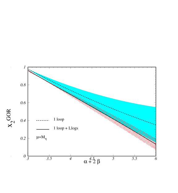
Figure 1: The GOR ratio at 1 loop including (continuous) and not including (dashed) the double logarithms. The scale is set to $\mu=M_{\eta}\pm 250$ MeV.

Eliminating the constant $A$ in favor of $\alpha$ and the ${\mathcal{L}}_{(2,1)}$ coupling $\xi^{(2)}$ in favor of $\beta$, one can express the GOR ratio of Eq. (1) as a function of the combination $\alpha+2\beta$,

$$x_{2}^{\mathrm{GOR}} =\left.x_{2}^{\mathrm{GOR}}\right|_{\mathrm{1-loop}}+\left[\frac{11}{60}-\frac{4169}{1080}(\alpha+2\beta)+\frac{5639}{1620}(\alpha+2\beta)^{2}\right.$$ (26)

$$\left.-\frac{121}{108}(\alpha+2\beta)^{3}\right]\left(\frac{M_{\pi}^{2}}{16\pi^{2}F_{\pi}^{2}}\log\frac{M_{\pi}^{2}}{\mu^{2}}\right)^{2}+O\left(M_{\pi}^{2}\hat{m}\log M_{\pi}^{2},M_{\pi}^{2}\hat{m}\right),$$

where $x_{2}^{\mathrm{GOR}}|_{\mathrm{1-loop}}$ is the $O(p^{4})$ result corresponding to Eq. (8). We are neglecting single-logarithmic and constant contributions which start at order $p^{5}$ in the generalized counting (cfr. discussion at the end of the previous section). The function (26) is shown in Fig. 1 as the full line (lower curve), together with the theoretical uncertainty, represented by the shaded band and estimated varying the ChPT renormalization scale $\mu$ by $\pm 250$ MeV around the value $\mu=M_{\eta}$, with the unknown l.e.c.’s considered as error sources, as in Eq. (9). In the lower band also, the error comes predominantly from the variation of the scale.

6. As it is clear from Fig. 1, the contribution of the double logarithms to $x_{2}^{\mathrm{GOR}}$ is quite large, specially in the “extreme” generalized case of large $\alpha+2\beta$, and tends to compensate the $O(p^{4})$ single logarithms. Still it is small enough in order to maintain the validity of the chiral expansion, the $O(p^{6})$ weighting about a half of the $O(p^{4})$ corrections. Moreover, the scale dependence is almost completely canceled by the double logarithms (cfr. the width of the shaded bands around the two curves). We stress that, at $O(p^{4})$ the scale-dependence arises because of our ignorance about the l.e.c.’s. It reflects the uncertainty about the scale at which the estimates (9) are supposed to hold. Indeed the effective theory, up to a given order of accuracy, defines a perfectly consistent theory, in the sense that the scale dependence from the chiral logarithms is compensated by the scale dependence of the l.e.c.’s [see Eq. (5)]. The non-renormalizability of the theory means that, as we want to increase the accuracy, we are forced to consider more and more l.e.c.’s, which implies a loss of predictive power of the theory. Therefore, if we knew the values of the l.e.c.’s at some scale, the complete $O(p^{4})$ result would be scale-independent. On the contrary, an $O(p^{6})$ calculation in the double logarithmic approximation introduces a scale dependence, which would be absorbed by the remaining $O(p^{6})$ corrections, including further unknown l.e.c.’s. It is remarkable that these two distinct sources of scale-dependence almost completely cancel with each other. This is certainly a signal of reduced theoretical uncertainty, although one must admit that the cancellation is fortuitous. A complete two-loop calculation with the generalized Lagrangian, would not be very useful, due to the flourishing of unknown l.e.c.’s. Double chiral logarithms are only part of this full two-loop calculation, but their contribution is known and unambiguous, apart from the scale-dependence. Moreover, there are reasons to believe that for some observables, namely the S-wave, isoscalar scattering length, or the parameter $\alpha$, they constitute -at least in the standard case, where a complete $O(p^{6})$ calculation is available- the bulk of the $O(p^{6})$ corrections [16]. We remind that the status of $\alpha+2\beta$ in this relationship is that of an observable quantity, extracted from the data using the full two-loop six-parametrical formula (7), with the constants $\lambda_{i}(\alpha,\beta)$ determined e.g. from the recent solution of the Roy equations [21]. This procedure yields, through Eq. (26), an experimental value for the two-flavor GOR ratio, with a theoretical uncertainty that we estimate to be twice the width of the lower band of Fig. 1. It is worth recalling that a GChPT fit to the old Rosselet data [22] gives $\alpha=2.16\pm 0.86$, $\beta=1.074\pm 0.053$ [12], where the error was dominated by the statistics, and no correlations between the two constants where taken into account. The experimental uncertainty will certainly be reduced by the new data from the $K_{e4}$ experiment, E865 at Brookhaven [9], with tenfold statistics compared to the Cern-Munich one [22]. A further increase in statistics is also expected in the planned NA48-2 $K_{e4}$ experiment at CERN, which will provide a very welcome complementary set of data in terms of different systematic uncertainties [23].

Acknowledgements.  This work was partly done at IFAE, Universitat Autonoma de Barcelona, under EEC-TMR program, Contract N. CT980169 (EURODA$\Phi$NE).

References

- [1] J. Stern, in: A.M. Bernstein, D. Drechsel, T. Walcher (Eds.), Chiral Dynamics: Theory and Experiment, Lecture Notes in Physics, Springer, Berlin, 1998, hep-ph/9712438; hep-ph/9801282.
-
[2]
B. Moussallam, Eur. Phys. J. C14 (2000), 111
; hep-ph/0005245.
S. Descotes, JHEP0103 (2001) 002. - [3] S. Descotes, L. Girlanda and J. Stern, JHEP 01 (2000), 41.
- [4] J. Stern, H. Sazdjian and N. H. Fuchs, Phys. Rev. D47 (1993), 3814;
-
[5]
N.H. Fuchs, H. Sazdjian and J. Stern, Phys. Lett. B269 (1991), 183;
M. Knecht, B. Moussallam and J. Stern, in The Second Dane Physics Handbook, eds. L. Maiani, G. Pancheri and N. Paver, 1995; hep-ph/9411259. - [6] J. Gasser and H. Leutwyler, Ann. Phys. (NY) 158 (1984), 142; Nucl. Phys. B250 (1985), 465.
- [7] S. M. Roy, Phys. Lett. B 36 (1971) 353.
- [8] G. Colangelo, J. Gasser and H. Leutwyler, Phys. Lett. B 488 (2000) 261; hep-ph/0103088.
- [9] P. Truol et al. [E865 Collaboration], hep-ex/0012012.
- [10] G. Colangelo, J. Gasser and H. Leutwyler, hep-ph/0103063.
-
[11]
L. Ametller, J. Kambor, M. Knecht and P. Talavera, Phys. Rev. D60 (1999), 094003.
L. Girlanda and J. Stern, Nucl. Phys. B575 (2000), 285. - [12] M. Knecht, B. Moussallam, J. Stern and N.H. Fuchs, Nucl. Phys. B457 (1995), 513;
- [13] M. Knecht, B. Moussallam, J. Stern and N.H. Fuchs, Nucl. Phys. B471 (1996), 445.
- [14] L. Girlanda, Nucl. Phys. Proc. Suppl. 86 (2000) 207.
- [15] L. Girlanda, M. Knecht, B. Moussallam and J. Stern, Phys. Lett. B409 (1997), 461.
- [16] G. Colangelo, Phys. Lett. B 350 (1995) 85.
- [17] S. Bellucci, J. Gasser and M.E. Sainio, Nucl. Phys. B423 (1994), 80.
- [18] J. Bijnens, G. Colangelo and G. Ecker, Phys. Lett. B 441 (1998) 437.
- [19] L. Girlanda, in LNF Spring School 2000, Frascati Physics Series, hep-ph/0007348.
- [20] J. Bijnens, G. Colangelo, G. Ecker, J. Gasser and M. Sainio, Phys. Lett. B374 (1996), 210; Nucl. Phys. B508 (1997), 263.
- [21] B. Ananthanarayan, G. Colangelo, J. Gasser and H. Leutwyler, hep-ph/0005297.
- [22] L. Rosselet et al., Phys. Rev. D 15 (1977) 574.
- [23] R. Batley et al., Proposal P253/CERN/SPSC.