Report of a Study on H2B

Prospect of a very long baseline neutrino oscillation experiment
HIPA to Beijing

1 Introduction

Neutrino oscillations, if neutrinos are massive, were first proposed by Pontecorvo [1] and by Maki, et al., [2], respectively, in the late 1950’s and early 1960’s. It is to date the only experimental indication of physics beyond the standard model (SM) that may provide a starting point to further expand the horizon of our most basic knowledge of nature. Historically neutrinos have played mostly passive roles in particle physics research. However, the observation of neutrino oscillations by the Super-Kamiokande experiment [3], which are corroborated by various other experiments, changed significantly the role of neutrinos and it has very profound implications for particle physics, astrophysics and cosmology. Neutrinos are the end product of the decays of almost all elementary particles, observed or proposed. They fill the universe as a relic background radiation similar to the photon as a finger print of the history of the universe. Now they are taking the center stage in particle physics research and their heightened fascination by physicists has just began.

Since it was proposed more than thirty years ago, the standard model of electroweak and strong interactions (SM) has been firmly established as the fundamental theoretical framework of elementary particles. Its applications straddles eleven orders of magnitude in energy range, from the atomic parity violation of 1 eV to the W, Z and top quark physics of hundreds of GeV. All high energy phenomenologies that have been scrutinized by experiments are found to agree with the predictions of the SM. The only missing piece is the Higgs particle. Even for that, a tentative gleam of its existence from the last LEP data [4] indicated that it may be what is expected from the SM. In reaching the present status of the SM, the IHEP’s BEPC program has made the important contribution in establishing the lepton universality which is a corner stone of the SM. In this “business as usual” state of affairs, evidence for neutrino oscillation and hence massive neutrinos gives light to the possibility of a new point of departure for post SM physics.

From the available neutrino oscillation data, we can already see some rich features of the neutrino sector. In analogy to the mass spectra of the quarks and charged leptons, there is a hierarchical structure in the mass square differences of the neutrinos. But in a departure from the feature of the quark sector, the mixing angles of the neutrinos are large, some probably maximal. Another intriguing aspect of the neutrino oscillations is that they are manifested macroscopically at terrestrial and solar distances. The physics of neutrino oscillation can be treated effectively by simple quantum mechanics. When finally confirmed, it will be an unique and elegant illustration of the effect of quantum interference at macroscopic scales.

Although the existing data offer strong indication of neutrino oscillations, the oscillation parameters have not been determined with sufficient accuracy. The unique signature of the flavor transmutation, i.e., the appearance of a flavor different from the original one, has not been convincingly observed. In the ongoing and next generation neutrino oscillation experiments under construction, some of the parameters will be probed with greater accuracy. But some other parameters may not yet be accessible. Hence more experiments designed to look for the missing information and to probe the known parameters with even greater accuracy are necessary.

One possible implication of the macroscopic manifestation of the neutrino oscillation is that the effect of the lepton flavor mixing may be very small in microscopic distances. Hence there are possibly very little observable effects to the conventional high energy physics parameters measured at microscopic distances, such as the charge lepton flavor changing neutral current [5]. This provides additional motivation for pursuing refined neutrino oscillation experiments so that the full implication of neutrino flavor mixing can be thoroughly investigated and understood, although the search for the effects at microscopic distances should be pursued.

This report summarizes the preliminary results of our study on a very long baseline (LBL) neutrino oscillation experiment, which uses the intensive conventional neutrino beam from the High Intensity Proton Accelerator (HIPA) [6], Japan, or the beam of a possible neutrino factory, delivered to a detector located in Beijing, China, tentatively called the Beijing Astrophysics and Neutrino Detector (BAND). HIPA to BAND (H2B) has a distance of 2100 km, which is eight times longer than the currently online LBL experiment, K2K, and three times longer than all of the three LBL experiments in construction: MINOS, ICARUS and OPERA. This very long baseline program has the distance to neutrino energy optimal for the atmospheric neutrino oscillation scale. It enables us to investigate some of the parameters that are not easily accessible by the above mentioned on-going and approved experiments. For a neutrino factory located in North America or Europe the distance to BAND is even much longer.

By the time this experiment becomes online some of the basic parameters related to the solar and atmospheric neutrino oscillations will be accurately determined. BAND will be in position to carry out a refined investigation of the neutrino oscillation parameters, such as the mixing parameters $\sin^{2}2\theta_{13}$, the matter effect and the sign of the dominant neutrino mass-squared difference. Additional important avenues of investigation include the effect of CP violation, some of the astrophysics measurements, the neutral current reactions that have scanty experimental information available to date, etc. The recent evidence of direct CP violation in the hadron sector [7] (and therefore evidence of non-vanishing phase in the CKM matrix) suggests that a non-vanishing phase angle may also exist in the lepton sector. Furthermore, the large mixing angles of the neutrinos makes it plausible to expect that the CP phase angle is likely large in the lepton sector.

This report is motivated by the discussions took placed at several workshops held at IHEP during the past two years. Several Physicists from Japan and USA joined their Chinese colleagues in the workshop held on May 25, 2000 [8]. As an outcome, an agreement was made to form two study groups, both consisting of experimentalists and theorists, to make independent studies of the physics potential of H2B. One group, coordinated by Dr. Kaoru Hagiwara, is made of physicists from KEK and the University of Kyoto and the other group, which is responsible for the present study report, includes physicists from China and USA. We believe our study so far and that of the KEK-Kyoto group [9] show that the physics of H2B is compelling and merits serious considerations for this very long baseline neutrino oscillation experiment. Further studies using more realistic neutrino beam parameters with detailed detector design are called for.

We envisage that the experimental programs outlined in this report will take a significant lead time to be fully implemented. The long lead time required is partly due to the R&D efforts of BAND but mainly constrained by the timeline of the neutrino beam, such as that from HIPA or a neutrino factory. We should also note that the long lead time is characteristic of modern large high energy physics experimental programs. Anticipating the long lead time, BAND will be constructed in the flexible modular approach and designed to do astrophysics experiment in the first stage of the program. In the intervening time, BAND will be thoroughly tested, enlarged and improved to be ready for the exciting physics of a LBL neutrino experiment.

In Sec. 2 we summarize the current experimental status of neutrino oscillations and the expectations of the new generation of experiments online and in construction. In Sec. 3 we summarize the theory of neutrino oscillations and list some of useful formulae. Section 4 outlines the fundamentals of the long baseline neutrino oscillation experiment and presents the result of a preliminary study of the physics expectations of H2B. Sec. 5 presents a preliminary design of a possible BAND detector as a concrete description of the physics results reachable at H2B.

A number of topics which are not covered by the present report will be the focus of the future studies, which involve a refined study of possible detector(s), study of other physics opportunities including those listed in Sec. 5.3, oscillation physics at even long oscillation distances that may involve BAND, and the comparison of H2B with other LBL experiments in construction. Topics such as the near detector, the neutrino beam design, and the choice of a far detector are expected to be the joint effort of a full collaboration with the participation of many physicists world wide, including the present study group, the critical participation from Japan, and from institutions of many other regions and countries.

2 Current experimental status of neutrino oscillations

In the following we review briefly the present experiments and the relevant data. For more details we refer to review articles available in the literature; we list a few in Ref. [10]. We do not claim to be exhaustive and apologize for the omission of any articles and experimental data. For an exhaustive list of neutrino experiments see the neutrino web-site in Ref. [11]. Since the interpretation of the data are mostly in the two-flavor scenario, we will first summarize the formalism of two-flavor oscillations in vacuum.

2.1 Two-flavor neutrino oscillations

We begin in the lepton flavor framework in which the charged lepton mass matrix is diagonalized. Define the two-flavor eigenstates $\nu_{\alpha}$ and $\nu_{\beta}$, and their mass eigenstates, $\nu_{1}$ and $\nu_{2}$ of masses $m_{1}$ and $m_{2}$, respectively. The flavor states and mass eigenstates are related by a mixing matrix $U$, which is an orthogonal transformation in two dimensions:

$$\left(\begin{array}[]{l}\nu_{\alpha}\\ \nu_{\beta}\end{array}\right)=U\left(\begin{array}[]{l}\nu_{1}\\ \nu_{2}\end{array}\right),~{}~{}~{}~{}~{}U=\left(\begin{array}[]{rr}\cos\theta&\sin\theta\\ -\sin\theta&\cos\theta\end{array}\right)$$ (1)

where $\theta$ is the mixing angle. The states are orthonormalized within their own spaces, i,e.,

$$<\nu_{j}|\nu_{k}>=\delta_{jk},~{}~{}~{}j,k=\alpha,\beta;~{}{\rm or}~{}1,2.$$ (2)

It should be noted that in an experiment, neutrinos are always produced as flavor eigenstates.

The time evolution of a flavor state can be simply expressed in terms of the time evolution of the mass eigenstates which enter into the flavor state at $t=0$,

$$\left(\begin{array}[]{l}\nu_{\alpha}(t)\\ \nu_{\beta}(t)\end{array}\right)=U\left(\begin{array}[]{l}\nu_{1}(t)\\ \nu_{2}(t)\end{array}\right)=U\left(\begin{array}[]{l}e^{-iE_{1}t}\nu_{1}\\ e^{-iE_{2}t}\nu_{2}\end{array}\right)=U\left(\begin{array}[]{ll}e^{-iE_{1}t}&0\\ 0&e^{-iE_{2}t}\end{array}\right)U^{\dagger}\left(\begin{array}[]{l}\nu_{\alpha}\\ \nu_{\beta}\end{array}\right),$$ (3)

Suppose the neutrino flavor state $\nu_{\alpha}$ is produced, then at time t we have

$$\nu_{\alpha}(t)=(\cos^{2}\theta e^{-iE_{1}t}+\sin^{2}\theta e^{-iE_{2}t})\nu_{\alpha}+\cos\theta\sin\theta(-e^{-iE_{1}t}+e^{-iE_{2}t})\nu_{\beta}.$$ (4)

The probability of finding the original flavor, referred to as the survival probability, is

$$P_{\nu_{\alpha}\rightarrow\nu_{\alpha}}=|<\nu_{\alpha}|\nu_{\alpha}(t)>|^{2} = 1-\sin^{2}(2\theta)\sin^{2}\left({E_{2}-E_{1}\over 2}t\right)$$ (5)

$$= 1-\sin^{2}(2\theta)\sin^{2}\left(1.267\Delta m^{2}({\rm eV^{2}}){L({\rm km})\over E_{\nu}({\rm GeV})}\right)$$

and the probability of finding the other flavor, called the appearance probability is

$$P_{\nu_{\alpha}\rightarrow\nu_{\beta}}=\sin^{2}(2\theta)\sin^{2}\left(1.267\Delta m^{2}({\rm eV^{2}}){L({\rm km})\over E_{\nu}({\rm GeV})}\right).$$ (6)

Here we take the approximation $E_{j}\approx|\vec{p}|+m_{j}^{2}/2E_{\nu}$ and denote $\Delta m^{2}=m^{2}_{2}-m^{2}_{1}$.

The characteristic behavior of this expression as a function of $\sin^{2}(2\theta)$ and $\Delta{m}^{2}$ is the following: for large $\Delta m^{2}$, the argument of the sine function is large and hence oscillates rapidly in even a very small energy range. The energy average of the sine function involved becomes ${1\over 2}$, hence we have

$$\sin^{2}(2\theta)\approx 2P_{\nu_{\alpha}\rightarrow\nu_{\beta}}.$$ (7)

For small $P_{\nu_{\alpha}\rightarrow\nu_{\beta}}$ and near $\sin^{2}(2\theta)=1$ the curve behaves like

$$\Delta{m}^{2}\approx{\sqrt{P_{\nu_{\alpha}\rightarrow\nu_{\beta}}}\over 1.267L/E_{\nu}}$$ (8)

Hence the effective probe in $\Delta{m}^{2}$ lies in the region

$${\sqrt{P_{\rm min}}\over 1.267L/E_{\nu}}<\Delta{m}^{2}<{\pi\over 1.267L/E_{\nu}}$$ (9)

This feature is true even for cases of more than two flavors of neutrinos. If the different mass squared differences are well separated, the effective probe of each mass squared is in the region of $L/E_{\nu}$ which satisfies the above relation.

2.2 Evidence of neutrino oscillations

The most convincing evidence of neutrino oscillations is given by the Super-Kamiokande (Super-K) experiment on atmospheric neutrinos [3]. The solar neutrino data provide the corroborative evidence of the oscillatory scenario. The reactor experiments have not seen any evidence of oscillations, but they provide strong constraints on some of the allowed regions of the oscillation parameters and are complementary to the atmospheric and solar data. The accelerator based short baseline experiments, LSND and KARMEN, are so far inconclusive. Fig. 1 summarizes the pertinent results of all experiments to date. The filled areas are allowed $\sin^{2}(2\theta)-\Delta{m}^{2}$ regions that provide the evidences of neutrino oscillations. Excluded regions lie above and to the right of the corresponding curves shown. Sensitivity curves of some of the future experiments are also shown.

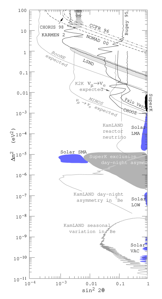
Figure 1: Summary of current experimental results on neutrino oscillations. Filled areas are allowed regions from the evidence of neutrino oscillations. Excluded regions are up and right of curves. Sensitivity curves of future experiments are also shown.

2.2.1 Atmospheric neutrinos

The atmospheric neutrino data are the so-called smoking gun of neutrino oscillations. They offer the strongest evidence of neutrino oscillations to date. The first indication of the “atmospheric neutrino anomaly” was observed in the 1960’s by experiments in South Africa and India and was confirmed during the 1980’s to 1990’s by IMB, Kamiokande, FREJUS, NUSEX, Soudan and MACRO experiments. The data are usually analyzed in terms of the double ratio, namely the observed over expected ratios of muon to electron neutrinos, to reduce the systematic error. Such ratio of ratios is measured to be about $0.60\pm 0.06$ instead of 1 as expected, indicating neutrino oscillations. The breakthrough came in the 1990’s when the Super-Kamiokande experiment went online. With a much larger statistical sample and broad energy range, they observed the following effects specific to neutrino oscillations [3]:

Zenith angle dependence: The down-ward($\theta=0^{\circ}$) and upward($\theta=180^{\circ}$) going neutrinos travel a distance varying from L=20 km to L=13000 km. The observation of zenith angle dependence of muon neutrino events consistent with the expected variation of oscillation probability as a function of L. For electron neutrinos, such variation was not observed and it is consistent with reactor neutrino experiments which found null oscillations of $\bar{\nu}_{e}$  [12, 13]. Such zenith angle dependence of $\nu_{\mu}$ has also been observed later by the Soudan 2 and the MACRO experiments.

Energy and L/E dependence: Muon neutrino events as a function of the neutrino energy and L/E have been observed and they are consistent with expected variation of neutrino oscillation probability. Again, electron neutrinos have no such variation.

East-west anisotropy: The Earth’s magnetic field, which deflects charged particles traveling in the atmosphere, affects the cosmic charge particles moving eastward differently from those moving westward. The neutrino flux model which takes into account the effect of the Earth’s magnetic field, is consistent with observed east-west anisotropy for horizontal going $\mu$-like and e-like event, supporting the neutrino oscillation interpretation[14].

The Super-K data allows for the $\nu_{\mu}\rightarrow\nu_{\tau}$ oscillation in a region shown in Fig. 1 at 90% CL. It is also reported recently [15] that the muon neutrino to a sterile neutrino, $\nu_{\mu}\rightarrow\nu_{s}$, as a dominant oscillation mode is excluded at the 99% confidence level (CL). Another exotic mechanism, i.e., the neutrino decay, although not completely excluded, is not a satisfactory explanation for the atmospheric neutrino data  [16].

2.2.2 Solar neutrinos

The “solar neutrino deficit” was first detected in 1968 [17] by the Homestake experiment and later confirmed by the Kamiokande, GALLEX, SAGE and Super-K experiments. The observed neutrino flux is only 1/3-1/2 of what was expected by the Standard Solar Model (SSM) depending on the neutrino energy. During the last decade, the understanding of the solar structure has been significantly improved, facilitating the analysis and interpretation of the solar neutrino data [18].

The only plausible explanation for this deficit is electron neutrino oscillation. Fig. 1 shows 4 allowed regions for $\nu_{e}$ oscillation into $\nu_{\mu}$ or $\nu_{\tau}$ in the $\Delta{m}^{2}-\sin^{2}(2\theta)$ space from results of all solar neutrino experiments:

Vacuum long wavelength oscillation solution (VAC): This solution assumes no matter effect and is also known as the ”just so” solution. The best fit gives a very small squared mass difference and nearly maximal mixing:

$$\Delta{m}^{2}~{}~{}\sim~{}~{}8\times 10^{-11}~{}{\rm eV}^{2},~{}~{}~{}~{}\sin^{2}(2\theta)~{}~{}\sim~{}~{}0.8.$$ (10)

In this solution the Earth-Sun distance is approximately half of an oscillation length, $L_{osc}=4\pi E_{\nu}/\Delta{m}^{2}$, which implies a significant dependence of the $\nu_{e}$ survival probability on the energy of the neutrino.

Small mixing angle MSW solution (SMA): In this solution the matter effect is included. The best fit of the data prior to the most recent Super-K data gives:

$$\Delta{m}^{2}\approx 5\times 10^{-5}~{}{\rm eV}^{2},~{}~{}~{}~{}\sin^{2}(2\theta)\approx 10^{-3}-10^{-2}.$$ (11)

Large mixing angle MSW solution (LMA): Again the matter effect is included and the allowed parameters are:

$$\Delta{m}^{2}\approx 2\times 10^{-5}~{}{\rm eV^{2}},~{}~{}~{}~{}\sin^{2}(2\theta)\approx 0.8.$$ (12)

Low mass solution (LOW): This is similar to the LMA case but with a much lower squared mass difference. The parameters are:

$$\Delta{m}^{2}\approx 8\times 10^{-8}~{}{\rm eV^{2}},~{}~{}~{}~{}\sin^{2}(2\theta)\approx 1.$$ (13)

For sterile neutrinos, only VAC and SMA solutions are allowed at 99% CL with similar parameters given above. However, recent Super-K results [19] have ruled out both the sterile neutrinos and the VAC and SMA solutions at 95% CL. The LMA and LOW are viable with the LMA being the favorable solution at 90% CL.

It should be remarked that the data do not rule out the oscillation of $\nu_{e}$ into two or more flavors with comparable probabilities. Furthermore, some analysis concluded that the solar neutrino data is still ambiguous and the SMA may still be viable[20]. Future data from SNO and BOREXINO as well as reactor data from KamLAND will be decisive for the determination of the solar neutrino oscillation parameters. Various possibilities of checking the solar neutrino problem can be found in Ref. [21].

2.2.3 Neutrino oscillation searches at nuclear reactors

Nuclear reactors are an intense and stable low energy source of $\bar{\nu}_{e}$, which is complementary to the solar neutrinos($\nu_{e}$). The beam emitted from the reactor is isotropic with an average energy around 3 MeV and an maximum energy of 10 MeV. The $\bar{\nu}_{e}$ flux is known within 2.7% when the reactor parameters are given. (For references, see Ref. [22].)

The two reactor neutrino experiments CHOOZ [12] and Palo Verde [13] both have a baseline of about 1 km and were recently completed. Null oscillation results have been reported and they excluded $\bar{\nu}_{e}\rightarrow\bar{\nu}_{x}$ oscillations in a region as shown in Fig. 1 at 90% CL. An important conclusion from the data of these experimental is that the atmospheric neutrino oscillation is not predominantly caused by the $\bar{\nu}_{\mu}\rightarrow\bar{\nu}_{e}$.

The future long baseline reactor neutrino experiment, KamLAND, may find the smoking gun for the solar neutrino problem. The detector consists of 1 kt of liquid scintillator and can detect $\bar{\nu}_{e}$ from all nuclear reactors in Japan with an event rate of 2/day. The characteristic baseline is 160 km and its sensitivity curve is shown in Fig. 1. If the solution to the solar neutrino deficit turns out to be LMA, KamLAND will be able to see the effect of neutrino oscillations, similar to the solar neutrino deficit.

2.2.4 Short baseline accelerator neutrino oscillation experiments

The accelerator neutrino experiments discussed below are low energy short baseline experiments which search for the oscillation $\nu_{\mu}(\bar{\nu}_{\mu})\rightarrow\nu_{e}(\bar{\nu}_{e})$. The results came from two experiments, LSND and KARMEN. The LSND experiment used a scintillator and Cherenkov detector with $L=29$ m and average neutrino energy $E_{\nu}=110$ MeV. It has the following results [23] before its completion in 1998:

Search for the $\bar{\nu}_{\mu}\rightarrow\bar{\nu}_{e}$ oscillation:

The $\bar{\nu}_{\mu}$ beam of LSND is produced from $\mu^{+}$ decay at rest. A total of 22 $\bar{\nu}_{e}$ events are observed via the reaction $\bar{\nu}_{e}P\rightarrow e^{+}n$, while only $4.6\pm 0.6$ events are expected to come from the background. A fit to the $e^{+}$ energy spectrum yields an excess of $51.8^{+18.7}_{-16.9}\pm 8.0$ events, corresponding to an oscillation probability of $(3.1^{+1.1}_{-1.0}\pm 0.5)\times 10^{-3}$ if interpreted as neutrino oscillations. The allowed region is shown in Fig. 1.

Search for the $\nu_{\mu}\rightarrow\nu_{e}$ oscillation:

In their later data sample, LSND has observed 40 events in $\nu_{\mu}\rightarrow\nu_{e}$ by using $\nu_{\mu}$ from $\pi^{+}$ decay in flight. The $\nu_{e}$ signal is detected via the charged current reaction $\nu_{e}C\rightarrow e^{-}X$. The expected backgrounds consist of $12.3\pm 0.9$ events from cosmic ray and $9.6\pm 1.9$ from other neutrino induced processes. Interpreted as neutrino oscillation, the excess of $18.1\pm 6.6$ events correspond to a $\nu_{\mu}\rightarrow\nu_{e}$ probability of $(2.6\pm 1.0)\times 10^{-3}$ which is consistent with the $\bar{\nu}_{\mu}\rightarrow\bar{\nu}_{e}$ oscillation probability given above. Since this is a $2.6\sigma$ effect, confirmation with higher statistics is necessary.

The KARMEN experiment uses a liquid scintillator detector with $L=17$ m at a comparable neutrino energy. KARMEN has not observed any oscillation signals. Its excluded region is also shown in Fig. 1. The data taking by KARMEN will be finished in 2001. Its sensitivity to $\bar{\nu}_{\mu}\rightarrow\bar{\nu}_{e}$ will be increased by a factor 1.7, but still cannot cover the whole LSND allowed region.

The Fermilab Mini-BooNE experiment which will be online in 2001, can cover the whole LSND allowed region. The Mini-BooNE $\nu_{\mu}$ beam, which has a broad band of 0.3-2 GeV and $\nu_{e}$ contamination of about 0.3%, is produced by the Fermilab 8 GeV, high intensity Booster Synchrotron proton beam. The 445 ton mineral oil detector is located 500 m from the neutrino source. The expected $\nu_{\mu}\rightarrow\nu_{e}$ oscillation suggested by the LSND data will produce 1500 excess events of the electron type which is many $\sigma$’s away from the statistical error of the experiment. The sensitivity curve is reported in Fig. 1.

We summarize in Table 1 the current status on the determination of the $\Delta{m}^{2}$ and $\sin^{2}(2\theta)$ parameters in the various types of experiments. Some of the most recent Super-K data are included. It should be emphasized again that the best values of the oscillation parameters are obtained assuming two-neutrino mixing.

Exp	Sources	Phenomenon	Recent results/remark
Reactor	$\bar{\nu}_{e}$	$\bar{\nu}_{e}$ survival	No oscill observed, rule out regions
			Expected future data from:
			KamLAND
Solar	$\nu_{e}$	$\nu_{e}$ deficit	Regions allowed: LMA & LOW & SMA & VAC
			Expected future data from:
			Super-K, SNO, BOREXINO
Atmospheric	$\nu_{\mu},\nu_{e}$	$\nu_{\mu}$ deficit	Dominant (@99% CL):
smoking gun			$\nu_{\mu}\rightarrow\nu_{\tau}$, $\nu_{\mu}\not\rightarrow\nu_{e},\nu_{s}$
			Regions allowed:
			$\Delta{m}^{2}_{\rm atm}=3.2(1.5-5)\times 10^{-3}$ eV2
			$\sin^{2}(2\theta_{\rm atm})=1(>0.88)$
			Expected future data from:
			Super-K, SNO
Accelerator	$\nu_{\mu},\bar{\nu}_{\mu}$	$\nu_{e},\bar{\nu}_{e}$ appear.	Region allowed by LSND:
SBL			$\Delta{m}^{2}_{\rm LSND}=0.2-1.0~{}{\rm eV^{2}}$
			$\sin^{2}(2\theta_{\rm LSND})=0.003-0.03$
			Controversial: some LSND allowed
			regions ruled out by KARMEN & Bugey
			Expect future data from:
			KARMEN, Mini-BooNE
Accelerator	$\nu_{\mu},\bar{\nu}_{\mu}$	$\nu_{\mu},\bar{\nu}_{\mu}$ survival	Preliminary results from K2K
hadron beam		$\nu_{e},\bar{\nu}_{e}$ appear	Three new exps online $\approx$ 2005
		$\nu_{\tau},\bar{\nu}_{\tau}$ appear	Determine $\nu$ parameters, CP(?)
Accelerator	$\nu_{\mu},\bar{\nu}_{\mu}$	$\nu_{\mu},\bar{\nu}_{\mu}$ survival	New generation of exps & accelerator
$\mu$-storage	$\nu_{e},\bar{\nu}_{e}$	$\nu_{\mu},\bar{\nu}_{\mu}$ appear	Accurate determination of $\nu$ parameters
		$\nu_{e},\bar{\nu}_{e}$ appear	Search for CP/T effect
		$\nu_{\tau},\bar{\nu}_{\tau}$ appear

Table 1: Summary of neutrino oscillation experiments.

2.3 Long baseline accelerator experiments

Below we discuss briefly four accelerator based LBL experiments: the online K2K and the three approved experiments, MINOS, ICARUS and OPERA. We also summarize the newly proposed LBL experiment J2K.

K2K-the online LBL experiment:

The K2K LBL neutrino oscillation experiment uses the meson neutrino beam produced at the KEK 12 GeV proton synchrotron. The average neutrino energy is 1.4 GeV which is below the tau lepton production threshold. It is expected to have $10^{20}$ protons on target (POT) in 5 years. The physics goals of the K2K are: (a) to check the $\nu_{\mu}$ survival probability, (b) to ensure that there is no large $\nu_{e}$ appearance probability, and (c) to determine the oscillation parameters. The far detector is the Super-Kamiokande located 250 km west of KEK. The experiment was commenced in April 1999 and the first neutrino event was observed on June 19, 1999, formally established the feasibility of this new type of high energy physics experiment.

Results from the first year of running corresponding to $2.29\times 10^{19}$ POT, were reported at ICHEP2000 [24]. A total of 27 $\nu_{\mu}$ interactions were observed inside the central detector, while $40.3^{+4.7}_{-4.6}$ were expected from the measurement of the front detector if $\nu_{\mu}$ is not subject to oscillation. The data is consistent with $\nu_{\mu}$ oscillation with $\Delta{m}^{2}$ approximately $1\times 10^{-3}$ eV², in agreement with the atmospheric result of Super-K. However the statistics is not significant enough to draw any firm conclusion. Nevertheless, it can be said that the data disfavor null oscillation at the 2$\sigma$ level. When more data are accumulated, an oscillation analysis of the neutrino energy spectrum can be performed, a stronger conclusion on oscillations can be made and the favorable parameter region may be obtained.

MINOS[25]: The neutrino beam comes from the 120 GeV Fermilab proton synchrotron and the detector is located in Soudan, Minnesota, USA. The distance between the beam source and the detector is 730 km. A brief summary of the experiment is given below:

• Goals: To (1) detect $\nu_{\mu}\rightarrow\nu_{\tau}$, (2) measure $\Delta{m}^{2}_{\rm atm}$ and $\sin^{2}(2\theta_{\rm atm})$ to 10%, and (3) search for the $\nu_{\mu}\rightarrow\nu_{e}$ component of the oscillation.

• Detector: 5 kt Iron-scintillation sandwich calorimeter with toroidal magnetic fields in the thin steel plates.

• Expected number of $\nu_{\mu}$ charge current interactions:
  Beam regime energy(GeV) CC events/kt-yr high 12 30000 medium 6 1450 low 3 450

ICARUS[26] The neutrino beam CNGS (CERN Neutrino Beam to Gran Sasso) is derived from the CERN 450 GeV proton synchrotron and the detector is located in the Gran Sasso underground laboratory. The average energy of the neutrino is less than 30 GeV and the distance traveled by the neutrino is 743 km.

• Goals: To do both LBL and atmospheric neutrino oscillation experiments. It can observe all three channels of neutrinos: $\nu_{e}$, $\nu_{\mu}$ and $\nu_{\tau}$ and is optimized for the observation of $\nu_{\tau}$.

• Detector: The detector is a liquid argon image detector. It involves new detector technology – liquid TPC – with modular structure. The first module of 600 t will be installed soon for solar neutrino and atmospheric neutrino physics.

• Excellent $e$ identification for the $\nu_{e}$ appearance experiment.

• $\nu_{\tau}$ appearance is a key physics goal. ICARUS expects 600 $\nu_{\tau}$ in the liquid target. For 4 years running the experiment sensitivity will be increased to $\Delta{m}^{2}_{\rm atm}=1.3\times 10^{-3}$ eV² and $\sin^{2}(2\theta_{23})=1.2\times 10^{-2}$.

OPERA[27]: The beam profile allows the CERN CNGS neutrino beam to supply neutrinos to both ICARUS and OPERA which is also located in Gran Sasso.

• Physics Goal: Optimized for $\nu_{\mu}\rightarrow\nu_{\tau}$ oscillation and excellent electron identification for the $\nu_{\mu}\rightarrow\nu_{e}$ search.

• Detector: Super module constructed out of individual scalable modules. Emulsion cloud chamber construction: massive dense material (Pb/Fe) plates as target plus thin emulsion sheet to track the $\tau$ decay, target section followed by a muon detector to reduce background to a very low level.

HIPA to Super-K (J2K) [28]: A new proposal has been made to use the proposed nuclear physics facility, the High Intensity Proton Accelerator (HIPA, formerly the JHF), to generate an intense neutrino beam with Super-K as the detector. HIPA, located about 60 km north-east of Tokyo, is a high intensity 50 GeV proton synchrotron accelerator, with an intensity of $1\times 10^{21}$POT/year. It will take 6 yeas to complete starting from 2001. We summarize the physics goals of J2K in the following:

• Observe $\Delta{m}^{2}$ to an accuracy of $2\times 10^{-4}$ eV².

• Assuming the dominant oscillation $\nu_{\mu}\rightarrow\nu_{\tau}$, $\sin^{2}(2\theta_{\mu})=\cos^{4}(\theta_{13})\sin^{2}(2\theta_{23})$ will be measured with an accuracy of 0.04.

• $\nu_{e}$ appearance search: to measure $\sin^{2}(2\theta_{e})=\sin^{2}(\theta_{23})\sin^{2}(2\theta_{13})$ to 0.05.

• $\nu_{\tau}$ appearance search: Very little hope unless $\Delta{m}^{2}_{32}$ is much larger than the current value of $3.5\times 10^{-3}$ eV^-3.

• search for the possible presence of sterile neutrino $\nu_{s}$ by neutral current events can provide a stringent limit on the existence of $\nu_{s}$.

Note that because of the distance, the matter effect is not significant and the oscillation effect is similar to that of the vacuum.

3 Theoretical introduction to neutrino oscillation

The experimental data available to date have provided the information needed for the construction of a generic framework for massive neutrinos. Let us first summarize the relevant experimental data before we embark on describing the possible theoretical scenarios that embody the data. If we accept all data as discussed in the proceeding section we see that there are three distinctive mass scales provided by the three categories of experiments: the LSND, atmospheric, and solar. The mass square difference (MSD) and the mixing angle in each category of experiments are given in Table 2. We list the current best values which are mostly from the Super-K collaboration for the atmospheric and solar neutrinos and the LSND collaboration for the SBL experiments. Coming from a single experiment, the LSND data have to be considered as tentative and require confirmation.

Category of Exp	MSD ($|\Delta{m}^{2}|~{}({\rm eV^{2}}$))	mixing angle $(\sin^{2}(2\theta))$
LSND	0.2-1	0.003-0.03
Atmospheric	$(1.5-5)\times 10^{-3}$	$>0.88$
Solar LMA	$2\times 10^{-5}$	$\approx 0.8$
SMA	$5\times 10^{-5}$	0.001-0.01
LOW	$8\times 10^{-8}$	$\approx 1$
VAC	$8\times 10^{-11}$	$\approx 0.8$

Table 2: Summary of mixing parameters of the three categories of neutrino oscillation experiments

The striking feature of the MSD pattern given in table 2 is that the three category of experiments provide three well-separated mass scales. This hierarchical structure of neutrino masses is similar to that of the quarks. It requires four distinct masses and hence the existence of at least four neutrino flavors. Therefore, accepting the LSND data immediately implies a non-trivial extension of the neutrino sector of the SM. The additional neutrino not contained in the SM is devoid of interactions with the SM electroweak gauge bosons, usually referred to as the sterile neutrino and denoted as $\nu_{s}$. If the LSND data are excluded, the three SM neutrino flavors are sufficient and no extension of the number of neutrinos is necessary. The latter case gives rise to the 3-neutrino scenario and the former the 4-neutrino scenario. Within either scenarios there are several cases which are different from one another by the ordering of the masses of the individual neutrino mass eigenstates. We will illustrate the different mass assignments below.

In view of the uncertainty of the LSND data, the discussion will be focused on the 3-flavor scenario. Comments on the 4-neutrino scenario will be made at the end of this section. For a detailed introductory theoretical review we refer to Ref. [29].

We define the neutrino states and masses by:        Flavor eigenstates: $\nu_{\alpha}$, $\nu_{\beta}$, $\nu_{\gamma}$…
      Mass eigenstates:    $\nu_{1}$, $\nu_{2}$, $\nu_{3}$…
       Masses:                $m_{1}$, $m_{2}$, $m_{3}$…

The column vector of the flavor states will be denoted as $[\nu_{\alpha}]$, and the column of mass eigenstates by $[\nu_{j}]$. The two sets of states are related by a unitary matrix U:

$$[\nu_{\alpha}] = U[\nu_{j}]$$

$$U \equiv \left(U_{\alpha j}\right)$$ (14)

To illustrate the different cases of the mass assignment let us consider the 3-flavor scenario. Because of the order of magnitude difference in their MSD, the solar and atmospheric data imply that two of the mass eigenstates lie closely in their mass values which we will assumed to be $\nu_{1}$ and $\nu_{2}$, with the third, assumed to be $\nu_{3}$, relatively far separated from the first two. Since the existing data give only the values of the MSD’s not their signs, the mass eigenstates cannot be unambiguously identified. Let us denote the mass order $m^{2}_{j}<m^{2}_{k}<m^{2}_{l}$ as the jkl-case, then there are four possible cases of the mass orders: 123, 213, 312 and 321. These four possibilities corresponding to four possible sign assignment to $\Delta{m}^{2}_{21}\equiv m^{2}_{2}-m^{2}_{1}$ and $\Delta{m}^{2}_{32}\equiv m^{2}_{3}-m^{2}_{2}$. Future experiments will have to find out which case is correct. Three of the four possible level assignments,123, 312 and 321 are shown in Fig. 2

Figure 2: Three possible level structures of the 3-neutrino scenario

3.1 Oscillation in vacuum

The formulae given in this subsection are valid for an arbitrary number of neutrino states.

3.1.1 Oscillation probabilities

The oscillation probabilities are functions of the mixing matrix elements $U_{\alpha j}$, the MSD’s $\Delta{m}^{2}_{kj}\equiv m^{2}_{k}-m^{2}_{j}$ with $m^{2}_{k}>m^{2}_{j}$, the neutrino energy $E_{\nu}$, and the oscillation length $L$. The oscillation probability of $\nu_{\alpha}\rightarrow\nu_{\beta}$ is given by

$$P_{\nu_{\alpha}\rightarrow\nu_{\beta}} = \delta_{\alpha\beta}-4\sum_{j<k}Y^{jk}_{\alpha\beta}\sin^{2}(\Delta_{kj})-2\sum_{j<k}J^{jk}_{\alpha\beta}\sin(2\Delta_{kj})$$ (15)

where

$$Y^{jk}_{\alpha\beta} \equiv Re\left(U_{\alpha j}U^{*}_{\alpha k}U^{*}_{\beta j}U_{\beta k}\right)$$

$$J^{jk}_{\alpha\beta} \equiv Im\left(U_{\alpha j}U^{*}_{\alpha k}U^{*}_{\beta j}U_{\beta k}\right)$$ (16)

$$\Delta_{kj} = 1.267\Delta m^{2}_{kj}({\rm eV}^{2}){L({\rm km})\over E_{\nu}({\rm GeV})}.$$

$Y^{jk}_{\alpha\beta}$ is symmetric in $jk$ and $\alpha\beta$, $J^{jk}_{\alpha\beta}$ is anti-symmetric in $jk$ and $\alpha\beta$:

$$Y^{jk}_{\alpha\beta} = Y^{kj}_{\beta\alpha}=Y^{jk}_{\beta\alpha}=Y^{kj}_{\alpha\beta}$$

$$J^{jk}_{\alpha\beta} = J^{kj}_{\beta\alpha}=-J^{jk}_{\beta\alpha}=-J^{kj}_{\alpha\beta}$$ (17)

$CP$ and $T$ violation effects will be exhibited if $J^{jk}_{\alpha\beta}\neq 0$.

The corresponding anti-neutrino oscillation probability can be obtained from the above expression by the replacement $U\rightarrow U^{*}$, giving

$$P_{\bar{\nu}_{\alpha}\rightarrow\bar{\nu}_{\beta}} = \delta_{\alpha\beta}-4\sum_{j<k}Y^{jk}_{\alpha\beta}\sin^{2}(\Delta_{kj})+2\sum_{j<k}J^{jk}_{\alpha\beta}\sin(2\Delta_{kj})$$ (18)

This replacement for the anti-neutrinos together with the symmetry relations of $Y^{jk}_{\alpha\beta}$ and $J^{jk}_{\alpha\beta}$ given above allows us to write down all the probability formulae for a given pair of neutrinos, $\nu_{\alpha}$ and $\nu_{\beta}$.

3.1.2 CP/T and CPT asymmetries

For a given pair of neutrino flavors, the probability $P_{\nu_{\alpha}\rightarrow\nu_{\beta}}$ is related to three other oscillations probabilities by CP, T and CPT transformations:

$$CP:~{}~{} P_{\nu_{\alpha}\rightarrow\nu_{\beta}}\rightarrow P_{\bar{\nu}_{\alpha}\rightarrow\bar{\nu}_{\beta}}$$

$$T:~{}~{}~{}~{} P_{\nu_{\alpha}\rightarrow\nu_{\beta}}\rightarrow P_{\nu_{\beta}\rightarrow\nu_{\alpha}}$$ (19)

$$CPT: P_{\nu_{\alpha}\rightarrow\nu_{\beta}}\rightarrow P_{\bar{\nu}_{\beta}\rightarrow\bar{\nu}_{\alpha}},$$

Effective measurements of symmetry violations can be made by the so-called asymmetries as defined below. For a given pair of flavors of neutrinos and anti-neutrinos, $\nu_{\alpha}$, $\nu_{\beta}$, $\bar{\nu}_{\alpha}$ and $\bar{\nu}_{\beta}$, six asymmetries can be defined for $\nu_{\alpha}\neq\nu_{\beta}$:

CP asymmetries:

$$A^{CP}_{\alpha\beta}={P_{\nu_{\alpha}\rightarrow\nu_{\beta}}-P_{\bar{\nu}_{\alpha}\rightarrow\bar{\nu}_{\beta}}\over P_{\nu_{\alpha}\rightarrow\nu_{\beta}}+P_{\bar{\nu}_{\alpha}\rightarrow\bar{\nu}_{\beta}}}={\sum_{j<k}J^{jk}_{\alpha\beta}\sin(2\Delta_{kj})\over 2\sum_{j<k}Y^{jk}_{\alpha\beta}\sin^{2}(\Delta_{jk})},$$ (20)

T asymmetries

$$A^{T}_{\alpha\beta}={P_{\nu_{\alpha}\rightarrow\nu_{\beta}}-P_{\nu_{\beta}\rightarrow\nu_{\alpha}}\over P_{\nu_{\alpha}\rightarrow\nu_{\beta}}+P_{\nu_{\beta}\rightarrow\nu_{\alpha}}}$$ (21)

CPT asymmetry

$$A^{CPT}_{\alpha\beta}={P_{\nu_{\alpha}\rightarrow\nu_{\beta}}-P_{\bar{\nu}_{\beta}\rightarrow\bar{\nu}_{\alpha}}\over P_{\nu_{\alpha}\rightarrow\nu_{\beta}}+P_{\bar{\nu}_{\beta}\rightarrow\bar{\nu}_{\alpha}}}$$ (22)

Three more asymmetries, one each corresponding to the above asymmetries, are obtained by the interchange of $\nu_{\alpha}$ and $\nu_{\beta}$.

The analytic expression of the oscillation probability assumes necessarily CPT symmetry and therefore gives vanishing CPT asymmetries. Hence given CPT symmetry there is only one independent asymmetry because of the identity,

$$A^{CP}_{\alpha\beta}=-A^{CP}_{\beta\alpha}=A^{T}_{\alpha\beta}=-A^{T}_{\beta\alpha}~{}~{}~{}{\rm with~{}CPT~{}invariance~{}in~{}vacuum}$$ (23)

due to the symmetry properties of $Y^{jk}_{\alpha\beta}$ and $J^{jk}_{\alpha\beta}$. However, the CPT asymmetries given above offer a simple way to check the underline assumptions of the CPT invariance in the neutrino sector and should be made.

In a neutrino factory, all six asymmetries can be measured for the $\nu_{\mu}$ and $\nu_{e}$ channels. But in the case of conventional meson-neutrino beams only the CP-asymmetries $A^{CP}_{\mu e}$ and $A^{CP}_{\bar{\mu}\bar{e}}$ are accessible.

3.2 The three-flavor scenario in vacuum

The three-flavor scenario is the experimentally favorable scenario. Although matter effects are always present in LBL experiments and their inclusion is necessary in order to extract precisely the oscillation parameters, the consideration of the vacuum case is nevertheless useful. It is a good approximation for experiments with shorter baselines. Moreover, it gives relatively simple expressions for the various oscillation probabilities which provides a more transparent picture of the physics. This allows us to look for the optimal experimental conditions to conduct a particular LBL experiment.

3.2.1 Basic formulae

The unitary mixing matrix can be parameterized as:

$$U = \left(\begin{array}[]{ccc}c_{12}c_{13}&c_{13}s_{12}&\hat{s}^{*}_{13}\\ -c_{23}s_{12}-c_{12}\hat{s}_{13}s_{23}&c_{12}c_{23}-s_{12}\hat{s}_{13}s_{23}&c_{13}s_{23}\\ s_{12}s_{23}-c_{12}c_{23}\hat{s}_{13}&-c_{12}s_{23}-c_{23}s_{12}\hat{s}_{13}&c_{13}c_{23}\end{array}\right)$$ (27)

where $s_{jk}=\sin(\theta_{jk})$, $c_{jk}=\cos(\theta_{jk})$, and $\hat{s}_{jk}=\sin(\theta_{jk})e^{i\delta}$. $\theta_{jk}$ defined for $j<k$ is the mixing angle of mass eigenstates $\nu_{j}$ and $\nu_{k}$ and $\delta$ is the CP phase angle. The presence of a non-vanishing $\delta$ will give rise to CP- and T-violation phenomena.

The CP/T-violation effect is given by the Jarlskog invariant [30]. From the unitarity condition it can be shown that there is only one Jarlskog invariant in the three-neutrino scenario. Hence the CP/T-violation part of all the oscillation probabilities are the same except for a possible sign difference. The Jarlskog invariant, denoted as $J(\delta)$ is defined by

$$J^{jk}_{\alpha\beta}=J(\delta)\sum_{\gamma,l}\epsilon_{\alpha\beta\gamma}\epsilon_{jkl}$$ (28)

where $(\alpha\beta\gamma)$ in the $\epsilon$-symbol run over the three neutrino flavors with $\epsilon_{e\mu\tau}\equiv+1$ and other permutations conventionally defined, and

$$J(\delta) = {1\over 8}c_{13}\sin(2\theta_{12})\sin(2\theta_{13})\sin(2\theta_{23})\sin(\delta).$$ (29)

The CP-violation term can be rewritten as

$$-2\sum_{j<k}J_{\alpha\beta}^{jk}\sin(2\Delta_{kj})=-8J(\delta)\sin(\Delta_{21})\sin(\Delta_{32})\sin(\Delta_{31})\sum_{\gamma}\epsilon_{\alpha\beta\gamma}$$ (30)

The explicit oscillation probabilities can be written done straightforwardly, including those for anti-neutrinos with the replacement $U_{\alpha j}\rightarrow U^{*}_{\alpha j}$.

3.2.2 Identification of mixing angles and MSD

In terms of the experimental data, the mixing and MSD parameters can be identified as follows:

$$\Delta{m}^{2}_{21} \equiv \Delta{m}^{2}_{solar}$$

$$\Delta{m}^{2}_{32} \equiv \Delta{m}^{2}_{atm}$$

$$\theta_{12} \equiv \theta_{solar}$$ (31)

$$\theta_{23} \equiv \theta_{atm}.$$

The ranges of values of the above parameters are given in Table 2 summarizing the experimental data given at the beginning of this section. The MSD $\Delta{m}^{2}_{31}$ is not independent,

$$\Delta{m}^{2}_{31}=\Delta{m}^{2}_{32}+\Delta{m}^{2}_{21}.$$ (32)

The third mixing angle, $\theta_{13}$ is not precisely measured. The CHOOZ collaboration gives an upper bound of the angle,

$$\sin^{2}(2\theta_{13})\leq 0.1.$$ (33)

3.2.3 Mass hierarchies, regimes of low and high mass scales

From the hierarchical structure of the MSD

$$|\Delta{m}^{2}_{31}|\approx|\Delta{m}^{2}_{32}|>>|\Delta{m}^{2}_{21}|,$$ (34)

we can classify LBL’s according to the neutrino energy and the baseline length. Let us define the MSD scale as the smallest MSD that gives the maximal oscillation, i.e., $\Delta_{jk}\approx\pi/2$

$$\Delta{m}^{2}_{\bf osc}({\rm eV}^{2})\equiv 1.240{E_{\nu}({\rm GeV})\over L({\rm km})}$$

which suggests that there are two relevant experimental regions: $\Delta{m}^{2}_{\rm osc}\approx\Delta{m}^{2}_{21}$ and $\Delta{m}^{2}_{\rm osc}\approx\Delta{m}^{2}_{31}$.

Low mass scale regime $\Delta{m}^{2}_{\rm osc}\approx\Delta{m}^{2}_{21}$

This region corresponds to the solar neutrino oscillation regime and for low $E_{\nu}$ and long $L$, where $\sin^{2}(\Delta{m}_{31})$ and $\sin^{2}(\Delta_{32})$ oscillate rapidly and can be replaced by ${1\over 2}$. Then the neutrino and anti-neutrino oscillation probabilities can be simplified as

$$P_{\nu_{\alpha}\rightarrow\nu_{\beta}} = \delta_{\alpha\beta}\left(1-2|U_{\alpha 3}|^{2}\right)+2|U_{\alpha 3}|^{2}|U_{\beta 3}|^{2}-4Y^{12}_{\alpha\beta}\sin^{2}(\Delta_{21})-2J^{12}_{\alpha\beta}\sin(2\Delta_{21})$$

$$P_{\bar{\nu}_{\alpha}\rightarrow\bar{\nu}_{\beta}} = \delta_{\alpha\beta}\left(1-2|U_{\alpha 3}|^{2}\right)+2|U_{\alpha 3}|^{2}|U_{\beta 3}|^{2}-4Y^{12}_{\alpha\beta}\sin^{2}(\Delta_{21})+2J^{12}_{\alpha\beta}\sin(2\Delta_{21})$$ (35)

In this mass scale regime, unless the baseline is very long, the neutrino energy will have to be low. The experimentally interesting measurements are the $\nu_{e}$ survival probability as in the solar neutrino oscillation experiment, and the $\nu_{\mu}\rightarrow\nu_{e}$ appearance probability:

$$P_{\nu_{e}\rightarrow\nu_{e}} = 1-{1\over 2}\sin^{2}(2\theta_{13})-c^{4}_{13}\sin^{2}(2\theta_{12})\sin^{2}(\Delta_{21}),$$

$$P_{\nu_{\mu}\rightarrow\nu_{e}} = {1\over 2}s^{2}_{23}\sin^{2}(2\theta_{13})+c^{2}_{13}c^{2}_{23}\sin^{2}(2\theta_{12})+2J(\delta)\sin(2\Delta_{21}).$$ (36)

The $\nu_{e}$ survive probability measures $\sin^{2}(2\theta_{13})$, $\Delta{m}^{2}_{21}$ and $c^{4}_{13}\sin^{2}(2\theta_{12})$ if the ratio $L/E_{\nu}$ can be varied so that the constant term and the oscillating term can be separately measured.

In this vacuum approximation the favorable distance to neutrino energy ratio for the LMA solution of the solar data of $\Delta{m}^{2}_{\rm solar}=2\times 10^{-5}$ eV² is $L/E_{\nu}=6.3\times 10^{4}$ km/GeV. For a neutrino energy of 3 MeV, which is in the average energy of the neutrino generated in a reactor, the distance is 190 km. As discussed in the preceding section, this is in the range of the KamLAND reactor experiment.

Note that the CP-violation term in the $\nu_{\mu}\rightarrow\nu_{e}$ oscillation is generally small as it is proportional to $\sin(2\theta_{13})$.

High mass scale regime $\Delta{m}^{2}_{\rm osc}\approx\Delta{m}^{2}_{31}\approx\Delta{m}^{2}_{32}$

This region is suitable for the terrestrial and accelerator neutrino oscillation experiments. In the leading approximation, the oscillation probabilities can be approximated by dropping the terms proportional to $\Delta{m}^{2}_{21}$. We will also ignore the CP-violation term in this approximation but will consider at the end of this discussion.

$$P_{\nu_{\alpha}\rightarrow\nu_{\beta}} \approx P_{\bar{\nu}_{\alpha}\rightarrow\bar{\nu}_{\beta}}$$ (37)

$$\approx \delta_{\alpha\beta}-4|U_{\alpha 3}|^{2}\left(1-|U_{\nu_{\beta}3}|^{2}\right)\sin^{2}(\Delta_{32}).$$

In more detail we have

$$P_{\nu_{\mu}\rightarrow\nu_{\mu}} \approx P_{\hat{\nu}_{\mu}\rightarrow\hat{\nu}_{\mu}}\approx 1-4c^{2}_{13}s^{2}_{23}(1-c^{2}_{13}s^{2}_{23})\sin^{2}(\Delta_{32}),$$

$$P_{\nu_{e}\rightarrow\nu_{e}} \approx P_{\hat{\nu}_{e}\rightarrow\hat{\nu}_{e}}\approx 1-\sin^{2}(2\theta_{13})\sin^{2}(\Delta_{32}),$$

$$P_{\nu_{\mu}\rightarrow\nu_{e}} \approx P_{\hat{\nu}_{\mu}\rightarrow\hat{\nu}_{e}}\approx s^{2}_{23}\sin^{2}(2\theta_{13})\sin^{2}(\Delta_{32}),$$ (38)

$$P_{\nu_{\mu}\rightarrow\nu_{\tau}} \approx P_{\hat{\nu}_{\mu}\rightarrow\hat{\nu}_{\tau}}\approx c^{4}_{13}\sin^{2}(2\theta_{23})\sin^{2}(\Delta_{32}),$$

$$P_{\nu_{e}\rightarrow\nu_{\tau}} \approx P_{\hat{\nu}_{e}\rightarrow\hat{\nu}_{\tau}}\approx c^{2}_{23}\sin^{2}(2\theta_{13})\sin^{2}(\Delta_{32}).$$

Due to the smallness of $\sin^{2}(2\theta_{13})$, in this experimental regime the appearance probabilities $P_{\nu_{\mu}\rightarrow\nu_{e}}$ and $P_{\nu_{e}\rightarrow\nu_{\tau}}$ are small, probably at a few percent level. However, because the mixing angle $\theta_{23}$ is near maximal, the appearance probability $P_{\nu_{\mu}\rightarrow\nu_{\tau}}$ can vary from close to 1 to zero when $L/E_{\nu}$ varies and it can provide a good measurement for the product $c^{4}_{13}\sin^{2}(2\theta_{23})$. The survival probability for $\nu_{e}$ stays large. But the survival probability for $\nu_{\mu}$ varies from close to 1 to near zero when $L/E_{\nu}$ varies.

Similar to the case of the low mass scale regime, the CP violation term is proportional to $\sin(2\Delta_{21})$ and is neglected in the above approximate expressions. But it can be identified as:

$$\Delta{P}^{CP}_{\nu_{\mu}\rightarrow\nu_{e}} = P_{\nu_{\mu}\rightarrow\nu_{e}}-P_{\bar{\nu}_{\mu}\rightarrow\bar{\nu}_{e}}$$ (39)

$$\approx +4J(\delta)\sin(2\Delta_{21})\sin^{2}(\Delta_{31})$$

and the corresponding CP asymmetry,

$$A^{CP}_{\mu e}\approx{\sin(2\theta_{12})c_{13}c_{23}\sin(2\Delta_{21})\over 2s_{23}\sin(2\theta_{13})}\sin\delta$$ (40)

This indicates that in order to be able to see the CP-violation in the $\nu_{\mu}\rightarrow\nu_{e}$ oscillation in this high mass scale regime, the solar mass scale $\Delta{m}^{2}_{21}$ can not be too small and it is favorable to have a large $L/E_{\nu}$ to maximize the product $\sin(2\Delta_{21})\sin^{2}(\Delta_{31})$.

Identifying $\Delta{m}^{2}_{\rm osc}\approx|\Delta{m}^{2}_{32}|=3.2\times 10^{-3}{\rm eV}^{2}$, then the effective experimental probe for a baseline length of 2100 km gives $E_{\nu}\approx 5.4$ GeV. This shows that the neutrino energy between 1 to 10 GeV from the H2B neutrino beam is in the optimal range for the probe of the atmospheric oscillation mass scale.

3.3 Oscillation in matter

The vacuum oscillation formulae is modified by the presence of matter along the path of the neutrino. When neutrinos propagate through matter, the SM neutrinos can interact with the quarks in the nucleons and electrons in the atoms to undergo both elastic and inelastic scatterings. The inelastic scattering and the elastic scatter off the forward direction will cause attenuation of the neutrino beam. Since the cross sections are extreme small, the attenuation are insignificant. However, the elastic scattering in the forward direction is a different matter. Although it does not change the direction of the neutrinos in the beam, it can modify the vacuum mixing angles and mass eigenvalues of the SM neutrinos. This matter effect is the well-known MSW effect [31], which is not CP symmetric, hence the modifications to the anti-neutrinos are different from those of the neutrinos. The matter effect on the electron neutrino is different from that on the muon or the tau neutrinos. It should also be noted that the matter effect is cumulative, in analogy with the propagation of light in a medium; the effect will be manifested more clearly when the length of propagation increases. Hence a clear detection of the matter effect will require a sufficiently long baseline. This intuitive conclusion is born out by the explicit calculation on the effect of the matter, and the H2B’s 2100 km baseline can provide explicit checks of the matter effect.

For the electron neutrino scattering through the matter, there are both charge and neutral current interactions. The muon and tau neutrinos subject only to neutral current interactions. For a sterile neutrino, since it does not interact with the SM gauge bosons, its propagation will not be affected by the presence of the matter. There are special considerations to simplify the calculation of the matter effect. We give some more details below. In the case of three-neutrino scenario without a sterile, the neutral current interaction is the same for all flavors. The effect of the elastic forward scattering due to neutral current is to give a common phase to all flavors. This has no effect on the oscillation and the neutrino current interaction can be ignored. However, the charge current interaction, which contributes only to the elastic scattering of electron neutrinos with the atomic electrons, has to be considered. Because the $e\nu_{e}$ and $e\hat{\nu}_{e}$ scatterings are different, matter effects on neutrinos and anti-neutrinos are different. Hence, the matter effect has to be carefully removed before the information on CP-violation can be extracted. The effect of T-violation can be investigated more readily, independent of the matter effect.

In a LBL experiment, as the neutrino traverses through the Earth, it encounters the Earth matter which may vary along the neutrino path. The density dependent matter effect is commonly dealt by the Schrödinger equation approach. The time evolution of the neutrino is equivalent to, and can be expressed as a differential equation in the distance of its propagation,

$$i{d\over dL}\nu_{\alpha} = {1\over 2E_{\nu}}\sum_{\beta}\left((\sum_{J}m^{2}_{j}U_{\alpha j}U^{*}_{\beta j})+A\delta_{\alpha e}\delta_{\beta e}\right)\nu_{\beta}$$ (41)

$$A = 2E_{\nu}a_{C}$$

$$a_{C} = \sqrt{2}G_{F}n_{e}=\sqrt{2}G_{F}N_{A}Y_{e}\rho$$

where $a_{C}$ is due to the charge current effect, $G_{F}$ is the Fermi constant, $n_{e}$ the number density of the electron, $N_{A}$ the Avogadro’s number, $\rho$(gm/cm³) the matter density in units of gram per cm³, and $Y_{e}$ the average of number of electrons per nucleon. The matter density $n_{e}$ and hence $\rho$ depend on $L$. For most of the Earth density, $Y_{e}$ can be taken as 1/2.

The above equation can be integrated numerically for the solution. Note that as mentioned before we have dropped the neutral current effect, which is common to all the three SM neutrinos and can be ignored. The expressions for anti-neutrinos can be obtained by the replacement: $U\rightarrow U^{*}$ and $A\rightarrow-A$.

For constant matter density, analytic expressions of the mixing parameters and oscillation probabilities expressed in terms of those of the vacuum quantities exist for the three-neutrino scenario [32, 33]. The explicit expressions for constant matter density are useful in estimating the magnitude of the matter and CP/T effects. Especially the approximate expressions are transparent in their physical meaning. The rest of this subsection is devoted to analytic expressions for the case of constant matter density.

3.3.1 Approximate expressions for constant matter density for high mass scale

In the following we list some relevant approximate expressions in the case of constant matter density in the leading oscillation for $\Delta{m}^{2}_{\rm osc}\approx\Delta{m}^{2}_{31}\approx\Delta{m}^{2}_{32}>>\Delta{m}^{2}_{21}$, which are relevant to terrestrial neutrino oscillation experiments and those for $L/E_{\nu}$ of the order of $(\Delta{m}^{2}_{32})^{-1}$, such as the H2B. Quantities that are subjected to modification by the approximated matter effect will be marked by the superscript “$m$”. The approximate expressions are simple enough that their physical meaning is clear.

A comparison of the approximate expressions with the exact one will be made at the end of the next subsection. The expressions given below, that set both $\Delta{m}^{2}_{21}$ and the CP phase $\delta$ to zero, are taken from Ref. [32]

$$P^{m}_{\nu_{\mu}\rightarrow\nu_{e}} \approx s^{2}_{23}\sin^{2}(2\theta^{m}_{13})\sin^{2}(\Delta^{m}_{32})$$

$$P^{m}_{\nu_{\mu}\rightarrow\nu_{\tau}} \approx \sin^{2}(2\theta_{23})\left(\sin^{2}(\theta^{m}_{13})\sin^{2}(\Delta^{m}_{21})+\cos^{2}(\theta^{m}_{13})\sin^{2}(\Delta^{m}_{31})-{1\over 4}\sin^{2}(2\theta^{m}_{13})\sin^{2}(\Delta^{m}_{23})\right)$$

$$P^{m}_{\nu_{\mu}\rightarrow\nu_{\mu}} = 1-P^{m}_{\nu_{\mu}\rightarrow\nu_{e}}-P^{m}_{\nu_{\mu}\rightarrow\nu_{\tau}}$$ (42)

$$P^{m}_{\nu_{e}\rightarrow\nu_{\tau}} \approx c^{2}_{23}\sin^{2}(2\theta^{m}_{13})\sin^{2}(\Delta^{m}_{32})$$

$$P^{m}_{\nu_{e}\rightarrow\nu_{e}} = 1-\sin^{2}(2\theta^{m}_{13})\sin^{2}(\Delta^{m}_{32})$$

where

$$\sin^{2}(2\theta^{m}_{13}) = {\sin^{2}(2\theta_{13})\over S^{2}}$$ (43)

$$S \equiv \sqrt{\left(\cos(2\theta_{13})-A/\Delta{m}^{2}_{31}\right)^{2}+\sin^{2}(2\theta_{13})}$$ (44)

$$\Delta^{m}_{32}\equiv S\Delta_{0},\hskip 12.91663pt\Delta^{m}_{31}\equiv{1\over 2}\left(1+{A\over\Delta{m}^{2}_{32}}+S\right)\Delta_{0},\hskip 12.91663pt\Delta^{m}_{21}\equiv{1\over 2}\left(1+{A\over\Delta{m}^{2}_{32}}-S\right)\Delta^{m}_{0}$$

with

$$\Delta^{m}_{0}\equiv{\Delta{m}^{2}_{32}L\over 4E_{\nu}}=1.267\Delta{m}^{2}_{32}({\rm eV^{2}}){L({\rm km})\over E_{\nu}({\rm GeV})}$$ (45)

The matter effect can be written explicitly for use in numerical simulation. A brief discussion of the earth density profile can be found in Sec. 4.1.3.

$$A = 0.7634\times 10^{-4}\rho({\rm g/cm^{3}})Y_{e}E_{\nu}({\rm GeV})$$ (46)

where $\mathrm{Y}_{e}=0.5$ is the number of electron per nucleon. Note that the matter resonance enhancement occurs at

$$E_{\nu}\approx 15({\rm GeV})\left(\Delta{m}^{2}_{31}({\rm eV^{2}})\over 3.5\times 10^{-3}({\rm eV^{2}})\right)\left({1.5({\rm g/cm^{3}})\over\rho({\rm g/cm^{3}})Y_{e}}\right)\cos(2\theta_{13})$$ (47)

For the H2B experiment, taking $\rho\approx 3~{}{\rm gm/cm^{3}}$, then the matter resonance occurs at $E_{\nu}\approx 15~{}{\rm GeV}$ which is in the range of the HIPA neutrino beam.

As already stated that the expressions of the corresponding anti-neutrino oscillation is obtained by the replacement $A\rightarrow-A$.

Because of the smallness of $\sin^{2}(2\theta_{13})$ the above probability expressions show that the $\nu_{\mu}\rightarrow\nu_{e}$ and $\nu_{e}\rightarrow\nu_{\tau}$ appearance probabilities are small, similar to the value in the vacuum case as discussed early. But they are enhanced due to the matter resonance effect. The $\nu_{\mu}\rightarrow\nu_{\tau}$ appearance probability as well as the $\nu_{\mu}$ and $\nu_{e}$ survival probabilities are large.

3.3.2 Exact results for constant matter density

In the following we list the exact expressions of 3-flavor mixing for constant matter density [33]. Quantities modified by the exact matter effect will be denoted by a superscript or subscript “$(m)$”. We rewrite the Schrödinger equation as

$$i{d[\nu^{(m)}_{\alpha}]\over dL} = H_{M}[\nu^{(m)}_{\alpha}]$$

$$H_{M} = H_{V}+{1\over 2E_{\nu}}AI_{ee}$$ (48)

$$= {1\over 2E_{\nu}}U(\Delta{M}^{2}+AU^{\dagger}{I_{ee}}U)U^{\dagger}$$

$$I_{ee} = \left(\begin{array}[]{ccc}1&0&0\\ 0&0&0\\ 0&0&0\end{array}\right)$$ (52)

The matter modified mass matrix, denoted by $\Omega$ can be diagonalized by a matrix $V$,

$$\Omega = \Delta{M}^{2}+AU^{\dagger}{I_{ee}}U\dagger$$ (53)

$$= VM^{2}_{(m)}V^{\dagger}$$

where

$$M^{2}_{(m)}=\left(\begin{array}[]{ccc}\lambda_{1}&&\\ &\lambda_{2}&\\ &&\lambda_{3}\end{array}\right)$$ (54)

contains the new mass square eigenvalues with the mass square eigenvalues [33]

$$\lambda_{1} = {1\over 3}\left[x-\sqrt{x^{2}-3y}\left(z+\sqrt{3(1-z^{2})}\right)\right]$$

$$\lambda_{2} = {1\over 3}\left[x-\sqrt{x^{2}-3y}\left(z-\sqrt{3(1-z^{2})}\right)\right]$$ (55)

$$\lambda_{3} = {1\over 3}\left[x+3\sqrt{x^{2}-3y}\right]$$

where

$$x = \Delta{m}^{2}_{21}+\Delta{m}^{2}_{31}+A$$

$$y = \Delta{m}^{2}_{21}\Delta{m}^{2}_{31}+A\left[\Delta{m}^{2}_{21}(1-|U_{e2}|^{2})+\Delta{m}^{2}_{31}(1-|U_{e3}|^{2})\right]$$ (56)

$$z = \cos\left({1\over 3}\cos^{-1}\left({2x^{3}-9xy+27\Delta{m}^{2}_{21}\Delta{m}^{2}_{31}|U_{e1}|^{2}}\over{2(x^{2}-3y)^{3/2}}\right)\right)$$

The elements of the diagonalization matrix $V$ are given by [33]

$$V_{jj}={N_{j}\over D_{j}},\hskip 21.52771ptV_{jk}={A\over D_{k}}(\lambda_{j}-\Delta{m}^{2}_{l1})U^{*}_{ej}U_{ek}$$ (57)

where $j\neq k\neq l$ takes the values 1, 2 and 3 and

$$N_{j} = (\lambda_{j}-\Delta{m}^{2}_{k1})(\lambda_{j}-\Delta{m}^{2}_{l1})-A\left[(\lambda_{j}-\Delta{m}^{2}_{k1})|U_{el}|^{2}+(\lambda_{j}-\Delta{m}^{2}_{l1})|U_{ek}|^{2}\right]$$

$$D^{2}_{j} = N^{2}_{j}+A^{2}|U_{ej}|^{2}\left[(\lambda_{j}-\Delta{m}^{2}_{k1})^{2}|U_{el}|^{2}+(\lambda_{j}-\Delta{m}^{2}_{l1})^{2}|U_{ek}|^{2}\right]$$ (58)

Now the Hamiltonian with the matter effect can be rewritten in the same form as the vacuum case:

$$H_{M} = {1\over 2E_{\nu}}U^{(m)}M^{2}_{(m)}U^{(m)\dagger}$$

$$U^{(m)} = (U^{(m)}_{\alpha j})=UV=\left(\sum_{k}U_{\alpha k}V_{kj}\right)$$ (59)

$$U^{(m)}_{\alpha j} = {(-1)^{j-1}\over D_{j}}\left[N_{j}U_{\alpha j}+AU_{ej}\left((\lambda_{j}-\Delta{m}^{2}_{k1})U^{*}_{el}U_{\alpha l}+(\lambda_{j}-\Delta{m}^{2}_{l1})U^{*}_{ek}U_{\alpha j}\right)\right]$$ (60)

Now the matter case can be written in the same expression as the vacuum case with the matter modified mixing matrix $U^{(m)}$ and the corresponding MSD’s,

$$\Delta^{(m)}{m}^{2}_{21} = {2\over 3}\sqrt{x^{2}-3y}\sqrt{3(1-z^{2})}$$

$$\Delta^{(m)}{m}^{2}_{32} = {1\over 3}\sqrt{x^{2}-3y}\left(3z-\sqrt{3(1-z^{2})}\right)$$ (61)

$$\Delta^{(m)}{m}^{2}_{31} = {1\over 3}\sqrt{x^{2}-3y}\left(3z+\sqrt{3(1-z^{2})}\right)$$

We define the oscillation argument for $j<k$:

$$\Delta^{(m)}_{kj}\equiv 1.267\Delta^{(m)}{m}^{2}_{kj}({\rm eV^{2}}){L({\rm km})\over E_{\nu}({\rm GeV})}$$ (62)

For the anti-neutrino, the corresponding quantities are obtained as in the neutrino case by the replacement:

$$U^{(m)}_{\alpha j} \rightarrow \bar{U}^{(m)}_{\alpha j}=U^{(m)*}_{\alpha j}(A\rightarrow-A),$$ (63)

$$\Delta^{(m)}_{kj} \rightarrow \bar{\Delta}^{(m)}_{kj}=\Delta^{(m)}_{kj}(A\rightarrow-A)$$ (64)

The oscillation probability expressions are similar to the vacuum case,

$$P^{(m)}_{\alpha\rightarrow\beta} = \delta_{\alpha\beta}-4\sum_{j<k}Re\left(U^{(m)}_{\alpha j}U^{(m)*}_{\alpha k}U^{(m)*}_{\beta j}U^{(m)}_{\beta k}\right)\sin^{2}(\Delta^{(m)}_{kj})$$ (65)

$$\hskip 18.51384pt-8J^{(m)}(\delta)\sum_{\gamma}\epsilon_{\alpha\beta\gamma}\prod_{j<k}\sin(\Delta^{(m)}_{kj})$$

$$P^{(m)}_{\bar{\alpha}\rightarrow\bar{\beta}} = \delta_{\bar{\alpha}\bar{\beta}}-4\sum_{j<k}Re\left(\bar{U}^{(m)}_{\alpha j}\bar{U}^{(m)*}_{\alpha k}\bar{U}^{(m)*}_{\beta j}\bar{U}^{(m)}_{\beta k}\right)\sin^{2}(\bar{\Delta}^{(m)}_{kj})$$ (66)

$$\hskip 18.51384pt+8\bar{J}^{(m)}(\delta)\sum_{\gamma}\epsilon_{\alpha\beta\gamma}\prod_{j<k}\sin(\bar{\Delta}^{(m)}_{kj})$$

where

$$J^{(m)}(\delta) = \left(\Delta{m}^{2}_{21}\Delta{m}^{2}_{31}\Delta{m}^{2}_{32}\over\Delta^{(m)}{m}^{2}_{21}\Delta^{(m)}{m}^{2}_{31}\Delta^{(m)}{m}^{2}_{32}\right)J(\delta)$$ (67)

$$\bar{J}^{(m)}(\delta) = J^{(m)}(\delta)(A\rightarrow-A)$$ (68)

$J(\delta)$ is the vacuum expression given before.

Unlike the vacuum case, the difference $P^{(m)}_{\nu_{\alpha}\rightarrow\nu_{\beta}}$ - $P^{(m)}_{\bar{\nu}_{\alpha}\rightarrow\bar{\nu}_{\beta}}$ contains both the CP-violation effect and the matter effect. However to estimate the CP angle we can calculate the T-violation asymmetry in which the matter effect and the CP phase can be separately isolated,

$$P^{(m)}_{\nu_{\alpha}\rightarrow\nu_{\beta}}-P^{(m)}_{\nu_{\beta}\rightarrow{\nu}_{\alpha}}=-16J^{(m)}(\delta)\sin(\Delta^{(m)}_{21})\sin(\Delta^{(m)}_{31})\sin(\Delta^{(m)}_{32})\sum_{\gamma}\epsilon_{\alpha\beta\gamma},$$ (69)

In the approximation of the last subsection, the T-symmetry is then given by

$$A^{(m)T}_{\nu_{\mu}\rightarrow\nu_{e}} = {{P^{(m)}_{\nu_{\mu}\rightarrow\nu_{e}}-P^{(m)}_{\nu_{e}\rightarrow\nu_{\mu}}}\over{P^{(m)}_{\nu_{\mu}\rightarrow\nu_{e}}+P^{(m)}_{\nu_{e}\rightarrow\nu_{\mu}}}}$$ (70)

$$\approx {8J^{(m)}(\delta)\sin(\Delta^{(m)}_{21})\sin(\Delta^{(m)}_{31})\over s^{2}_{23}\sin^{2}(2\theta^{m}_{13})\sin(\Delta^{(m)}_{32})}$$

which can be measured at a neutrino factory but not with a meson-neutrino beam.

Let us comment briefly on the validity of the approximate expressions given in the preceding subsection. In the H2B region, i.e., $L=2100$ km and $E_{\nu}$ in the range of 1-10 GeV, the approximate expressions are good to within a few percent for the various oscillation probabilities. In the energy regime of a few hundred MeV and lower, the term proportional to $\sin^{2}(\Delta_{21})$ is no longer negligible and it becomes eventually the dominant contribution. Then the approximate expressions are no longer valid.

3.4 Comment on the four-neutrino scheme

Although the current results disfavor strongly the dominance of the oscillation of $\nu_{e}\rightarrow\nu_{s}$ as the mechanism for the solar neutrino deficit and $\nu_{\mu}\rightarrow\nu_{s}$ for the atmospheric neutrino anomaly, a sizable contribution of the sterile neutrino to these oscillations is allowed [34]. For a summary of the 4-neutrino fit of the various data, see Ref. [35]. Because of the far reaching implications of such a scenario, it is worthwhile to maintain an interest in the scenario. If the LSND result is accepted, there are clear three different MSD’s squared mass differences of the order of magnitude:

$\Delta{m}^{2}_{\rm solar}\leq 10^{-5}~{}{\rm eV}^{2}$

$\Delta{m}^{2}_{\rm atm}\approx 10^{-3}{\rm eV}^{2}$

$\Delta{m}^{2}_{\rm LSND}\approx 1{\rm eV}^{2}$ which calls for at least four different neutrino masses. This has the implication that a right-handed or sterile neutrino exists. The existing data favors the so-called 2+2 scheme. However, another possibility, i.e., the so-called 3+1 scheme is not completely ruled out [34]. In the 2+2 scheme the 4 neutrino mass eigenstate states are divided into 2 groups each containing 2 levels. Within each group the mass separation is relatively small in comparison with separation between the groups. Therefore, one group gives the solar energy scale and the other the atmospheric scale. The scale between the groups gives the LSND oscillation. In the 3+1 scheme, the 4 states also divided into two groups. One group contains 3 mass eigenstates and the other group one state. The 3-eigenstate group provides the solar and atmospheric oscillation scales similar to the 3-flavor scenario. The MSD between the groups is the LSND scale. Let us label the mass eigenstates as $\nu_{0}$, $\nu_{1}$, $\nu_{2}$ and $\nu_{3}$. Three possible level structures for the 2+2 scheme are given in Fig. 3

Figure 3: Three possible level structures of the 4-neutrino scenario

The three squared mass difference are identified as:

$\Delta{m}^{2}_{\rm solar}=|\Delta{m}_{01}|$

$\Delta{m}^{2}_{\rm atm}=|\Delta{m}^{2}_{32}|$

$\Delta{m}^{2}_{\rm LSND}=|\Delta{m}^{2}_{31}|\approx|\Delta{m}^{2}_{21}|$, etc.

Again the different level structures have different signs for $\Delta{m}^{2}_{kj}$, $j<k$. In a complete determination of the neutrino parameters, the signs of $\Delta{m}^{2}_{kj}$ have to be determined.

The four-neutrino scheme is generally treated numerically with the Schrödinger equation. In this case there are six mixing angles and six CP phases. Three of the CP phases can give rise to measurable CP-violation effects in oscillation experiments. For an explicit parameterization of the mixing matrix we refer to Ref. [5]. The matter effect is more complicated than in the three-neutrino scenario because neutral current interactions have to be included since they are no longer common to all neutrino flavors. The CP effect can be sizable and may be easier to detect.

4 Fundamentals of LBL experiments and physics of H2B

The neutrino oscillation is a system with a limited number of degrees of freedom, it yet exhibits a multitude of interesting phenomena. In the 3-flavor scenario, the system consists of 2 MSD, three mixing angles and one CP phase that determine the different survival and appearance probabilities. The numerous neutrino experiments, solar, atmospheric, reactor, and short baseline, are mostly looking at the survival probabilities and often use neutrino beams that exist in nature. In most cases there is no way to tune the neutrino beams for more desirable experimental results. Hence it is difficult to obtain all of the oscillation parameters for the entire mixing matrix, either because the statistics are too low, or the energy is not suitable. In long baseline experiments, the neutrino beams are produced in the accelerator according to certain physics criteria so that the experiment can be conducted in a controlled fashion. Ideally, the distance between the neutrino source and the detector can be chosen to maximize the physics output. The distance can be hundreds or thousand kilometers to allow high energy neutrino beams to be used and still offer suitable $L/E_{\nu}$ values. The LBL experiments promise to allow for detailed analysis of the oscillation parameters so as to provide a complete picture of the neutrino oscillations.

We will first briefly summarize some of the fundamentals of the LBL experiment and then the possible physics that can be investigated at H2B. More pertinent simulation studies will be carried out with a specific detector later.

4.1 Fundamentals of LBL experiments

Long baseline neutrino oscillation experiments are not conventional high energy physics experiments. Due to the extremely weak interaction cross section of neutrinos and the long baseline between the neutrino source and the detector, both the neutrino beam intensity and the detector mass must be maximized in order to have the desired statistics. New technologies for both accelerators and detectors may be required. In the following we discuss briefly some of the fundamentals of the LBL experiment before we start to discuss the specific neutrino beam that may be available and the detectors that are necessary to achieve the physics goals.

4.1.1 Neutrino beams

There are two kinds of accelerator neutrino beams: the so-called neutrino factory from muon decays and the conventional neutrino beam from meson decays. While meson-neutrino beams have been built by many laboratories and the remaining technological challenge is to increase the total power of the primary proton beam, the neutrino factory is a completely new concept and there are still a host of technical issues to be worked out.

Neutrino factory: The neutrino factory delivers a neutrino beam which contains comparable amount of $\nu_{\mu}$ ($\bar{\nu}_{\mu}$) and $\bar{\nu}_{e}$ ($\nu_{e}$) obtained from the $\mu^{-}(\mu^{+})$ decay in a $\mu$-storage ring.

$$\mu^{-}(\mu^{+})\rightarrow\nu_{\mu}(\bar{\nu}_{\mu})+\bar{\nu}_{e}(\nu_{e})+e^{-}(e^{+})$$ (71)

Note that the presence of both the muon and electron neutrinos is not a problem because they have opposite chiralities and therefore will not be a background to each other if the detector can distinguish between positive and negative electric charges. A description of the neutrino factory can be found in [36].

The neutrino flux at baseline L from a neutrino factory of unpolarized muon of energy $E_{\mu}$ is given by

$${d\Phi\over dE_{\nu}}=\left\{\begin{array}[]{lll}2x^{2}_{f}(3-2x_{f}){n_{0}\gamma^{2}\over\pi L^{2}E_{\mu}}&for&\nu_{\mu}\\ 12x^{2}_{f}(1-x_{f}){n_{0}\gamma^{2}\over\pi L^{2}E_{\mu}}&for&\nu_{e}\end{array}\right.$$ (72)

where $x_{f}=E_{\nu}/E_{\mu}$, $n_{0}$ is the number of useful decaying muon, and $\gamma=E_{\mu}/m_{\mu}$ with $m_{\mu}$ being the mass of the muon. The average neutrino energies are given by

$$\langle E_{\nu_{\mu}}\rangle = 0.7E_{\mu}$$

$$\langle E_{\nu_{e}}\rangle = 0.6E_{\mu}$$ (73)

Two scenarios of the number of neutrinos in a beam have been considered: $n_{0}=6\times 10^{19}/$year for an entry level factory and $n_{0}=6\times 10^{20}/$year for a high performance factory. For a discussion of the neutrino beam spread in a neutrino factor together with some sample plots, see Ref. [37]

Meson-neutrino beam: Neutrinos from a meson source are obtained from decays of pions and kaons produced by collisions of primary protons with nuclear target. The secondary meson beam produced by the collision is sign selected and then focused by a magnetic field. Mesons are then transported to a vacuum decay pipe, whose length depends on the desired energy of the neutrino, and finally striking a hadron absorber further downstream. The primary neutrino or anti-neutrino beam consists mostly of the muon flavor from $\pi^{\pm}$ and $K^{\pm}$ decays in the decay pipe but some impurities of electron neutrinos are expected due to a finite branching ratio of $\pi^{\pm}$, $K^{\pm}$ and $\mu^{\pm}$ decaying into electrons and positrons plus their associated neutrinos. For example, the NuMI muon neutrino beam at Fermilab contains 0.6% electron neutrinos. As for the energy spectrum of the beam, it can be a wide-band beam covering a broad range of energies, or narrow band beam with a selected, well-defined energy range.

The neutrino flux at the detector site is determined by the baseline L, the number of primary protons on target (POT), the proton energy $E_{p}$ and the neutrino energy $E_{\nu}$. The following empirical formula [38] describes the meson production from a proton beam on a nuclear target:

$$x_{M}{d\sigma\over dx_{M}} = 2\pi\int x_{M}E_{p}{d^{3}\sigma\over dp^{3}}P_{t}dP_{t}$$ (74)

$$= 2\pi\int{B(1-x_{M})^{A}{1+5e^{-Dx_{M}}\over(1+P^{2}_{t}/C)^{4}}}P_{t}dP_{t}$$

$$= (1-x_{M})^{A}(1+5e^{-Dx_{M}})$$

where $E_{p}$ is the proton beam energy, $p$ the proton 3-momentum, $x_{M}$ is the Feynman x-variable defined as the momentum of the secondary meson divided by the momentum of proton. A, B, C, and D are numerical parameters which are different for different secondary particles. Table 3 gives their fitted values for $\pi^{+},\pi^{-},K^{+}$, and $K^{-}$, taken from Ref.[38]. For a wide band beam, we can take Eq.(72), i.e., the $\mathrm{E}_{\nu}^{2}/L^{2}$ behavior, to account for the transverse momentum spread due to pion decays. The neutrino flux can then be written as

$$\Phi(E_{\nu},L)\propto{E_{\nu}(1-x_{\nu})^{A}(1+5e^{-x_{\nu}D})\over L^{2}}$$ (75)

where we take $x_{M}\simeq x_{\nu}\equiv 2E_{\nu}/E_{p}$. It is interesting to note that this simple formula can account for the beam design of MINOS at various energies as discussed in Sec. 2.3. We should remark that there is a more complete treatment [39] for the energy spectrum for the meson-neutrino beam. However the difference with the above express for $E_{\nu}>1$ GeV is very small. Owing to its simpler form, we continue to use the above expression in the following calculations.

	A	B	C	D
$\pi^{+}$	2.4769	5.6817E-2	0.57840	3.0894
$\pi^{-}$	3.5648	5.0673E-2	0.68725	5.0359
$K^{+}$	1.7573	6.3674E-3	0.81771	5.6915
$K^{-}$	5.4924	4.1712E-3	0.89038	2.2524

Table 3: Numerical parameters for meson-neutrino energy spectrum

4.1.2 Dip angle

To deliver the neutrino beam to the detector that is $L$ (direct) distance away, the beam has to point downward at a dip angle $\theta_{\rm dip}$ from the horizontal plane given by

$$\theta_{\rm dip}=\sin^{-1}\left(L\over 2r_{\rm E}\right),$$ (76)

where $r_{\rm E}=6371$ km is the average earth radius. This is the same dip angle of the hadron decay pipe in the case of meson-neutrino beam. The dip angle is 1.1^∘ for K2K, 3.3^∘ For MINOS, ICARUS and OPERA. H2B has an oscillation length of 2143 km and the dip angle is 9.6^∘.

4.1.3 The Earth matter density profile

The solid earth is made of three major parts, the crust, mantle and core. The density increases with increasing depth $D$ from the Earth surface. However, there are local variations of the earth density. A widely used model for the earth is the Preliminary Reference Earth Model (PREM) provided by Dziewonski and Anderson [40]. We list in Table 4 the earth densities versus the radius and the depth from the Earth surface, where $x\equiv r/r_{E}$, r is the radius at a given depth. The density is in units of g/cm³ and the radius and depth in km. The densities given are of course the average densities. The extrapolation formulas are valid in the sublayers where the mass densities vary. The actual densities at a given depth is given in the square bracket. The earth density profile [41] is also plotted as a function of the distance along a diameter from one end on the earth surface to the opposite end as given by the solid curve in Fig. 4 [42].

region	radius r(km)	depth D(km)	extrapolation[density] (g/cm3)
ocean	6371	0	[1.0200] ([2.6000])
(continent)	6368	3	[1.0200] ([2.6000])
crust	6368	3	[2.6000]
	6356	15	[2.6000]
	6356	15	[2.9000]
	6346.6	24.4	[2.9000]
LID	6346.6	24.4	+0.6914x [3.808]
	6291	80	2.6910 [3.3747]
low velocity zone	6291	80	+0.6914x [3.3747]
	6151	220	2.6910 [3.3595]
transition zone	6151	220	-3.8045x [3.4358]
	5971	400	7.1089 [3.5433]
	5971	400	-8.0298x [3.7238]
	5771	600	11.2494 [3.9758]
	5771	600	-1.4836x [3.9758]
	5701	670	5.3197 [3.9921]
lower mantle	5701	670	-6.4761x+5.6283x2-3.0807x3 [4.3807]
	5600	771	7.9565 [4.4432]
	5600	771	-6.4761x+5.6283x2-3.0807x3 [4.4432]
	3630	2741	7.9565 [5.4915]
	3630	2741	-6.4761x+5.5283x2-3.0807x3 [5.4915]
	3480	2891	7.9565 [5.5665]
outer core	3480	2891	-1.2638x-3.6426x2-5.5281x3 [9.9035]
	1221.5	4260.5	12.5815 [12.1582]
inner core	1221.5	4260.5	-8.8381x2 [12.764]
	0	6371	13.0885 [13.0885]

Table 4: Earth density versus the radius; $x\equiv r/r_{E},D\equiv r_{E}-r$.

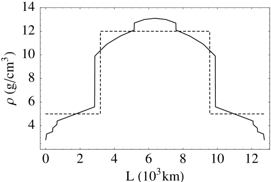
Figure 4: Earth density profile.

For very long baseline experiment with high energy neutrino beams, such as H2B, the matter effect will be important. The deepest reach of a neutrino beam is given by

$$D=r_{E}(1-\sqrt{1-{L^{2}\over 4r^{2}_{E}}})$$ (77)

which is 80 km in the case of H2B. The neutrino beam will go through mostly the earth crust but also part of the upper mantle. On the average the earth density along the path of H2B varies from 2.6 g/cm³ at the initial beam entry into the earth to 3.8 g/cm³ in the middle point of the beam and back to 2.6 g/cm³ when the beam exits into the detector. Local variation along the beam path has to be carefully modeled in order to investigate the CP effect.

4.1.4 Interaction cross sections

The detection of the neutrino flavor is through the charge current interaction. For the neutrino energy which is small compared to the mass of the W-boson, the charge current cross sections for the electron and muon neutrino are given by

$$\sigma^{(e,\mu)}_{\nu N} = 0.67\times 10^{-38}{\rm cm}^{2}E_{\nu}(\rm GeV)$$ (78)

$$\sigma^{(e,\mu)}_{\bar{\nu}N} = 0.34\times 10^{-38}{\rm cm}^{2}E_{\nu}(\rm GeV)$$ (79)

For the tau neutrino, the above expression is subject to a threshold suppression. The threshold for the production of the tau is

$$E_{T}=m_{\tau}+{m_{\tau}^{2}\over 2m_{N}}=3.46~{}{\rm GeV}$$ (80)

The charge current production cross section of the $\tau$ is usually given numerically as a function of the neutrino energy. We fit the numerical cross sections from the threshold to 100 GeV and obtained the following expression

$$\sigma^{(\tau)}_{\nu N}/\sigma^{(\mu)}_{\nu N}={(E_{\nu}-E_{T})^{2}\over c_{0}+c_{1}E_{\nu}+c_{2}E^{2}_{\nu}}\theta(E_{\nu}-E_{T}),$$ (81)

where $c_{0}=-84.988$, $c_{1}=18.317$, and $c_{2}=1.194$. As shown in Fig. 5, the fit is good to within 3%. The difference occurs mostly in the neutrino energy region of 20-40 GeV. The fit is valid for $E_{\nu}\geq 4.0$ GeV.

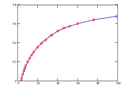
Figure 5: A fit of the numerical ratio of the $\tau$ to $\mu$ charge current production cross section from the threshold to 100 GeV. The boxes are the data and the dotted curve is the fit. The horizontal axis is the neutrino energy in GeV and the vertical axis is the ratio of $\tau$ to $\mu$ production cross sections.

4.1.5 Neutrino Statistics

The number of neutrino events of $E_{\nu}$ and flavor $\beta$, from a neutrino beam of energy $E_{\nu}$ and flavor $\alpha$, to be observed at a baseline L is given by

$$N_{\nu_{\beta}}=\Phi(E_{\nu},L)\sigma(E_{\nu})P_{\alpha\rightarrow\beta}(E_{\nu},L),$$ (82)

where $\Phi(E_{\nu},L)$ is the neutrino flux including the detector size, $P_{\alpha\rightarrow\beta}(E_{\nu},L)$ is the oscillation probability and $\sigma(E_{\nu})$ the neutrino charge current cross section. Without committing to an accelerator and a detector design we can not specify the absolute neutrino statistics precisely. In the simulation presented in the next subsection, we will take an arbitrary normalization. From the discussion of Subsection 4.1.1, we see that the relative energy spectrum of the neutrino beam is specified. For the neutrino factory we will not specify the parent muon energy, hence each neutrino energy is taken to be the average energy of the neutrino beam energy as also discussed in Subsection 4.1.1. Then we have

$$N_{\nu_{\beta}} \propto \left\{\begin{array}[]{ll}{E^{3}_{\nu}\over L^{2}}P_{\alpha\rightarrow\beta}(E_{\nu},L)&{\rm neutrino-factory}\\ (1-x_{\nu})^{A}(1+5e^{-x_{\nu}D}){E^{2}_{\nu}\over L^{2}}P_{\alpha\rightarrow\beta}(E_{\nu},L)&{\rm meson-neutrino}\end{array}\right.$$ (85)

The dependence of $N_{\nu_{\beta}}$ on $L$ and $E_{\nu}$ depends on the behavior of the oscillation probability on these variables. The general behavior of oscillation probability is complicated because it is a function of two MSD’s which appear in oscillating functions. However, for LBL with neutrino energy of order GeV and varying within a relatively small range, the contribution of the solar MSD, $\Delta{m}^{2}_{21}$, is small and proportional to $(L/E_{\nu})^{2}$. The leading contribution comes from the atmospheric MSD scale, $\Delta{m}^{2}_{32}$. Hence for $L/E_{\nu}<<(\Delta{m}^{2}_{32})^{-1}$, $P_{\alpha\rightarrow\beta}(E_{\nu},L)\propto L^{2}/E^{2}_{\nu}$. For $L/E_{\nu}\approx(\Delta{m}^{2}_{32})^{-1}$, $P_{\alpha\rightarrow\beta}(E_{\nu},L)$ is not subject to the $(L/E_{\nu})^{2}$ suppression except for the energy dependence entering the matter effect which modifies the mixing angles. Therefore, we have

$$N_{\nu_{\beta}} \propto \left\{\begin{array}[]{ll}E&{\rm for~{}}L/E_{\nu}<<(\Delta{m}^{2}_{32})^{-1}\\ {E^{3}\over L^{2}}&{\rm for~{}}L/E_{\nu}\approx(\Delta{m}^{2}_{32})^{-1}\end{array}\right.$$ (88)

for neutrino factories and

$$N_{\nu_{\beta}} \propto \left\{\begin{array}[]{ll}(1-x_{\nu})^{A}(1+5e^{-x_{\nu}D})&{\rm for~{}}L/E_{\nu}<<(\Delta{m}^{2}_{32})^{-1}\\ (1-x_{\nu})^{A}(1+5e^{-x_{\nu}D}){E^{2}_{\nu}\over L^{2}}&{\rm for~{}}L/E_{\nu}\approx(\Delta{m}^{2}_{32})^{-1}\end{array}\right.$$ (91)

for conventional neutrino beams by using Eqs.(72,75,78,79). Naively from the above, we expect to have better results at higher energy for neutrino factories while at lower energy for conventional beams. In the following, we will discuss in detail where are the best place to do measurements for some of the most important quantities.

4.2 Physics of H2B

In this subsection we will summarize in general terms the physics goals of H2B and compare its capability with those of different distances [43]. A preliminary study of the sensitivity of BAND on the measurements of the physics goals, with a specific detector as an example, will be discussed in the next section. We assume that in 5 to 8 years the solar neutrino mixing parameters will be more accurately determined. Also the parameters of the atmospheric neutrinos will be narrowed down. A broad range of physics goals can be defined for H2B, depending on the neutrino beam either from a meson source or from a $\nu$-factory. We emphasize the advantages of an experiment at a very long baseline, such as 2100 km, and the neutrino energy in the GeV range. To limit the scope of the analysis, we will only discuss the scenario of three neutrinos with MSW-LMA as the solution to the solar neutrino problem. Some of the following results will appear in Ref. [44]. The earth density has been chosen to be a constant of $\mathrm{\rho}=3~{}g/cm^{3}$, other mixing parameters are set as follows: $\Delta m^{2}_{32}=\Delta m^{2}_{31}=3\times 10^{-3}eV^{2}$, $\Delta m^{2}_{21}=5\times 10^{-5}eV^{2}$, $\theta_{12}=\theta_{23}=45^{0}$, and $\theta_{13}=7^{0}$. The leptonic CP phase $\delta$ is set to be $90^{\circ}$ and the matter effect constant $A/E_{\nu}$ is $2.3\times 10^{-4}eV^{2}/GeV$.

4.2.1 Mixing probability $\sin^{2}2\theta_{13}$

The oscillation probability $P(\nu_{\mu}\rightarrow\nu_{e})$ is a direct measurement of $\sin^{2}2\theta_{13}$ since $P(\nu_{\mu}\rightarrow\nu_{e})\propto\sin^{2}2\theta_{13}$. Of course $\sin^{2}2\theta_{13}$ also appears in $\nu_{e}\rightarrow\nu_{\tau}$ channel, but experimentally it is much more difficult. The statistical significance of $P(\nu_{\mu}\rightarrow\nu_{e})$ can be measured by the figure of merit defined by $P(\nu_{\mu}\rightarrow\nu_{e})/\delta P(\nu_{\mu}\rightarrow\nu_{e})$, where the error $\delta P(\nu_{\mu}\rightarrow\nu_{e})$ can be written as

$$\delta P=\delta N_{s}/\Phi\sigma=\delta(N-N_{b})/\Phi\sigma=\sqrt{\delta^{2}N+\delta^{2}N_{b}}/\Phi\sigma=\sqrt{N+r^{2}N^{2}_{b}}/\Phi\sigma.$$ (92)

Here N is the total candidate event, $N_{s}$ the signal event and $N_{b}$ the background event. The uncertainty in estimating the background is represented by a parameter $\mathrm{r}$, which is typically a few percent. In this report, we will use $r=0.1$. If we express $N_{b}=f\Phi\sigma$, where $\mathrm{f}$ is the background fraction in terms of neutrino events of the original flavor, we have

$$\delta N_{s}=\sqrt{P\Phi\sigma+f\Phi\sigma+r^{2}f^{2}\Phi^{2}\sigma^{2}}.$$ (93)

It is clear that if $P~{}<<~{}f$, there will be no sensitivity for the given measurement of the signal. Generally speaking, at shorter baseline when P is small, the effect of backgrounds is larger. Typical values of $f$ for water Čerenkov detectors are a few percent. Contributions to $f$ from the beam are at the level of 0.6% for meson-neutrino beams. We conservatively choose $f=0.03$ for conventional beams and $f=0.02$ for neutrino factories.

The figure of merit $P/\delta P$ can then be written as

$${P\over\delta P}={P\over{\delta N_{s}/\Phi\sigma}}={P\over\sqrt{{P+f\over\Phi\sigma}+r^{2}f^{2}}}.$$ (94)

Using the analytical formula for oscillations in Sec. 3.3.2 and Eqs.(72) and (78-79), this quantity can be plotted as a function of the neutrino energy E at different baselines.

To see the role played by the background let us first consider the figure of merit by ignoring the background, i.e., setting $f=0$. The results are given in Fig. 6a and b. As shown in Fig. 6a there is no $E_{opt}$ for a given L where the figure of merit is a maximum for $E_{\nu}\leq 20$ GeV for a neutrino factory. It would be more advantageous to work at higher neutrino energies and shorter baselines. For a conventional neutrino beam, there is an $E_{opt}$ associated to each L, and the smaller baseline seemed to have higher figure of merit as shown in Fig. 6b.

Figure 6: Figure of merit for $\sin^{2}2\theta_{13}$ measurement at a) neutrino factories without backgrounds, b) meson-neutrino beams without backgrounds, c) neutrino factories with f=0.02 and r=0.1, and d) meson-neutrino beams with f=0.03 and r=0.1.

The above picture is changed when the effect of the background is taken into account. As shown in Figs. 6c and 6d, an $E_{opt}$ exists for each distance with the figure of merit increasing with the oscillation distance for both the conventional neutrino beams and neutrino factories. For the neutrino factory, the figure of merit of the longer baselines such as 2100 km and 3000 km are much higher than the shorter baselines of 700 km and 300 km. For the meson-neutrino beam the longer baseline is also better although the difference is not so prominent in comparison with the case of neutrino factory. This comparison of Figs 6c and 6d with Figs 6a and 6b demonstrates the importance of the effect of the background in deciding the relative merits at different baselines.

Since neutrino beams generally have a broad energy distribution, the correct figure of merit should integrate over the expected energy spectrum. While at neutrino factories, the neutrino energy spectrum is well represented by Eq.(72), it is more complicated for meson-neutrino beams since specific beam design can alter significantly the energy spectrum. As a general rule of thumb, it is always better to have a larger width of the figure of merit curve. To this respect, it is advantageous at longer baselines as shown in Fig. 6. A simple trial effort using Eq.(72) for neutrino factories and Eq.(75) for meson-neutrino beams shows that L=2100 km is preferred.

4.2.2 Leptonic CP phase $\delta$

As discussed in the Introduction, the leptonic CP phase for neutrinos may be large as the neutrino mixing angles are large. The CP phase $\delta$ can be measured by looking at the difference of the oscillation probability between $P(\nu_{\mu}\rightarrow\nu_{e})$ and $P(\bar{\nu}_{\mu}\rightarrow\bar{\nu}_{e})$ or between $P(\nu_{e}\rightarrow\nu_{\mu})$ and $P(\nu_{\mu}\rightarrow\nu_{e})$. While the former has to have the matter effect removed in order to obtain the CP effect, the later, under the assumption of CPT conservation, allows the isolation of the matter from the CP effect, but it can only be done at a neutrino factory.

We define

$$\Delta P=P(\nu_{\mu}\rightarrow\nu_{e})-P(\bar{\nu}_{\mu}\rightarrow\bar{\nu}_{e})\equiv P-\bar{P}$$ (95)

and the pure CP phase can be obtained by subtracting the matter effect $\Delta P(\delta)-\Delta P(\delta=0)$. The error of $\Delta P$ can be written as

$$\delta(\Delta P)=\sqrt{\delta^{2}P+\delta^{2}\bar{P}}=\sqrt{{\delta^{2}N_{s}\over\Phi^{2}_{\nu}\sigma^{2}_{\nu}}+{\delta^{2}\bar{N}_{s}\over\Phi^{2}_{\bar{\nu}}\sigma^{2}_{\bar{\nu}}}}$$ (96)

and the figure of merit for the leptonic CP phase measurement can be written as

$${\Delta P(\delta)-\Delta P(\delta=0)\over\delta(\Delta P)} = {\Delta P(\delta)-\Delta P(\delta=0)\over\sqrt{{P+f\over\Phi_{\nu}\sigma_{\nu}}+r^{2}f^{2}+{\bar{P}+f\over\Phi_{\bar{\nu}}\sigma_{\bar{\nu}}}+r^{2}f^{2}}}$$ (97)

using Eq.(93). Fig. 7a shows the figure of merit for neutrino factories with backgrounds as discussed above. It is clear from the figure that, for every L, there is an optimum energy for CP phase $\delta$ measurement. Once L/E is fixed at the optimum energy, the sensitivity to CP phase $\delta$ is a factor of 2 better at L=2100 km than that at L=300 km. The sensitivity to CP for conventional neutrino beams is shown in Fig. 7b by using Eq.(75) and (78-79). A similar optimum energy also exists, but the sensitivity at L=2100 km is about 20% lower than that at L=300 km at their respective peak values due to unfavorable beam divergence at long distance. The integrated figure merit, however, still favors the longer baseline.

Figure 7: Figure of merit for CP phase measurement at a) neutrino factories with f=0.02 and r=0.1, and b) meson-neutrino beams with f=0.03 and r=0.1.

Similar conclusions can be obtained by using other quantities, such as $\Delta P/(P+\bar{P})$, $P/\bar{P}$, $P(\nu_{e}\rightarrow\nu_{\mu})-P(\nu_{\mu}\rightarrow\nu_{e})$, etc.

¿From Eq.(97), we can see that the figure of merit is roughly proportional to $1/\sqrt{P}$. This means that it is much better to measure the CP phase when P is small, i.e., in the $\nu_{e}-\nu_{\mu}$ or $\nu_{e}-\nu_{\tau}$ channel, but not the $\nu_{\mu}-\nu_{\tau}$ channel, thanks to the small term $\sin^{2}2\theta_{13}$ in $P(\nu_{e}-\nu_{\mu})$ and $P(\nu_{e}-\nu_{\tau})$. In reality, we can only use the $\nu_{e}-\nu_{\mu}$ channel due to higher experimental efficiencies.

4.2.3 Sign of $\Delta m^{2}_{32}$

Since the vacuum oscillation probability is an even function of $\Delta{m}^{2}_{kj}$, the presence of the matter effect is necessary in order to measure the sign of $\Delta m^{2}_{32}$. The simplest way is to compare the measured probability $P(\nu_{\mu}\rightarrow\nu_{e})$ with expected $P^{+}(\nu_{\mu}\rightarrow\nu_{e})$ and $P^{-}(\nu_{\mu}\rightarrow\nu_{e})$ where, $P^{+}$ assumes $\Delta m^{2}_{32}>0$ and $P^{-}$ for $\Delta m^{2}_{32}<0$. The channel $\bar{\nu}_{\mu}\rightarrow\bar{\nu}_{e}$ may be more advantageous to use if $\Delta m^{2}_{32}<0$. This measurement can only be done if $\sin^{2}2\theta_{13}$ is sizable and the $\nu_{e}$ or $\bar{\nu}_{e}$ appearance signal is statistically significant. Other channels, such as the $\nu_{\mu}\rightarrow\nu_{\mu}$ survival channel, are less sensitive due to the very small matter dependent terms. It has been suggested [45] that total muons from all channels at neutrino factories, e.g. the $\nu_{e}(\bar{\nu}_{e})\rightarrow\nu_{\mu}(\bar{\nu}_{\mu})$ appearance and $\nu_{\mu}(\bar{\nu}_{\mu})\rightarrow\nu_{\mu}(\bar{\nu}_{\mu})$ survival channels, be used to reduce systematic errors. Here we confine ourselves only to relatively simple approaches to illustrate the statistical importance at different baselines. The figure of merit in the present case can be written as

$${P^{+}-P^{-}\over\delta P}={P^{+}-P^{-}\over\delta N_{s}/\Phi\sigma}={P^{+}-P^{-}\over\sqrt{{P^{+}f\over\Phi\sigma}+r^{2}f^{2}}}.$$ (98)

Figure 8: Figure of merit for the sign of $\Delta m^{2}_{32}$ at a) neutrino factories with f=0.02 and r=0.1, and b) meson-neutrino beams with f=0.03 and r=0.1.

Fig. 8 shows this figure of merit as a function of energy at different baselines for a) neutrino factory and b) conventional neutrino beams. It is clear from the plots that in both cases, it is much better to have an experiment at L=2100 than at L=300 km.

4.2.4 Matter effect

The matter effect can be measured by looking at the difference between $\nu_{\mu}\rightarrow\nu_{e}$ and $\bar{\nu}_{\mu}\rightarrow\bar{\nu}_{e}$, although non-zero CP phase $\delta$ can alter the result by as much as 20%. The survival channels $\nu_{\mu}\rightarrow\nu_{\mu}$ and $\bar{\nu}_{\mu}\rightarrow\bar{\nu}_{\mu}$ are not very effective for the present consideration since matter effects in these channels appear only in the non-leading terms. It is better to use the channels that involve $\nu_{e}$ or $\bar{\nu}_{e}$.

Denote $P_{1}=P(\nu_{\mu}\rightarrow\nu_{e})$ and $P_{2}=P(\bar{\nu}_{\mu}\rightarrow\bar{\nu}_{e})$, the relevant figure of merit can be written as

$${P_{1}-P_{2}\over\delta(P_{1}-P_{2})} = {P_{1}-P_{2}\over\sqrt{\delta^{2}P_{1}+\delta^{2}P_{2}}}={P_{1}-P_{2}\over\sqrt{{{\delta^{2}N_{\mu}\over\Phi^{2}_{\nu}\sigma^{2}_{\nu}}+{\delta^{2}N_{\bar{\mu}}\over\Phi^{2}_{\bar{\nu}}\sigma^{2}_{\bar{\nu}}}}}}={P_{1}-P_{2}\over\sqrt{{P_{1}+f\over\Phi_{\nu}\sigma_{\nu}}+r^{2}f^{2}+{P_{2}+f\over\Phi_{\bar{\nu}}\sigma_{\bar{\nu}}}+r^{2}f^{2}}}.$$ (99)

Fig. 9 shows this figure of merit as a function of energy at different baselines for a) neutrino factory and b) conventional neutrino beams. It is clear from the plots that in both cases, it is much better to have an experiment at L=2100 than at L=300 km.

Figure 9: Figure of merit for the matter effect at a) neutrino factories with f=0.02 and r=0.1, and b) meson-neutrino beams with f=0.03 and r=0.1.

4.2.5 Precision measurement of $\Delta m^{2}_{32}$ and $\sin^{2}2\theta_{23}$

Although $\Delta m^{2}_{32}$ and $\sin^{2}2\theta_{23}$ have been measured at super-K and hopefully will be confirmed by K2K, MINOS, OPERA and ICARUS, it is still interesting to measure them at different baselines and possibly improve the precision. $\Delta m^{2}_{32}$ and $\sin^{2}2\theta_{23}$ can be directly related to the survival probability $P(\nu_{\mu}\rightarrow\nu_{\mu})$. The figure of merit can be written as

$${1-P\over\delta P}={1-P\over{\delta N_{s}/\Phi\sigma}}={1-P\over\sqrt{{P+f\over\Phi\sigma}+r^{2}f^{2}}}.$$ (100)

Fig. 10 shows the figure of merit at different baseline for a) neutrino factories and b) conventional neutrino beams. Since the background for muon identification is generally much smaller than in the case of the electron, we use f=0.01 for both neutrino factories and conventional beams. A nice peak corresponding to $\Delta m^{2}_{32}L$ where the oscillation is at a maximum can be found and its position is a good measure of $\Delta m^{2}_{32}$. It is clear that for neutrino factories it is better at 2100 km and for conventional beams, it is better at 300 km. The integrated figure of merit at $L=2100$ km is much higher than that at $L=300$ km for a neutrino factory. For the meson-neutrino beam the longer baseline is also higher.

Figure 10: Figure of merit for $\Delta m^{2}_{32}$ and $\sin^{2}2\theta_{23}$ at a) neutrino factories with f=0.01 and r=0.1, and b) meson-neutrino beams with f=0.01 and r=0.1.

4.2.6 $\nu_{\mu}\rightarrow\nu_{\tau}$ Appearance

The appearance of $\nu_{\tau}$ from a $\nu_{\mu}$ beam is an unambiguous proof of the $\nu_{\mu}\rightarrow\nu_{\tau}$ oscillation. Precision measurement of this oscillation probability is crucial in establishing the oscillation patterns and in determining whether or not $\nu_{\mu}\rightarrow\nu_{\tau}$ is the only dominant oscillation mode or there are still rooms for the $\nu_{\mu}\rightarrow\nu_{s}$ oscillation. Although we expect that in the next few years, K2K and/or OPERA will observe the production of $\tau$ because of the large $\nu_{\mu}\rightarrow\nu_{\tau}$ probability, it is desirable that BAND possesses a good $\tau$ identification capability. We assume that our detector can identify the $\tau$ based on statistics methods, namely event selection via signature on kinematics. The figure of merit can be written as

$${P(\nu_{\mu}\rightarrow\nu_{\tau})\over\delta P(\nu_{\mu}\rightarrow\nu_{\tau})}={P\over{\delta N_{s}/\Phi\sigma}}={P\over\sqrt{{P+f\over\Phi\sigma}+r^{2}f^{2}}}.$$ (101)

Fig. 11 shows this figure of merit as a function of energy at different baselines for a) neutrino factories and b) conventional neutrino beams. Although the neutrino beam does not contribute to the background, it is expected to be high after event selection. Hence we set f=0.03 for both neutrino factories and meson-neutrino beams. Due to the threshold of tau production, the experiment has to be done at $\mathrm{E}_{\nu_{\mu}}>4GeV$. That is different from what is needed for CP phase measurements at $\mathrm{L}<2000$ km. While shorter baseline seems better at a given energy, it is generally better to run only one energy for all measurements to accumulate enough statistics. To this end, L=2100 km is much better than that at L=300 km.

Figure 11: Figure of merit for tau appearance at a) neutrino factories with f=0.03 and r=0.1, and b) meson-neutrino beams with f=0.03 and r=0.1.

4.2.7 Exotic scenarios

• Sterile neutrinos Although the Super-K collaboration has demonstrated that the sterile neutrino is excluded at the 99% CL to be the dominant oscillation partner of $\nu_{\mu}$, it has not ruled out a sizable oscillation probability for $\nu_{\mu}\rightarrow\nu_{s}$ [46]. The presence of $\nu_{\mu}\rightarrow\nu_{s}$ oscillation will lead to a suppressed survival probability $\nu_{\mu}\rightarrow\nu_{\mu}$ at $E\sim 15$ GeV due to matter effects. Then very long baseline experiments, such as H2B, will have the advantages to search for the suppression.

• Neutrino decay The possibility of neutrino decay as an explanation of Super-K’s atmospheric neutrino observations has not been completely excluded [16]. However, it has been predicted that there is a significant difference on the $\nu_{\mu}$ survival probability $P(\nu_{\mu}\rightarrow\nu_{\mu})$ between the oscillation and decay scenarios at $L/E_{\nu}({\rm km/GeV})\sim 400$. Therefore the figure of merit to make the discrimination of the two scenarios is equivalent to that given in Fig. 10. Hence we expect that K2K and MINOS will be able to answer the neutrino decay question in the near future before we are online.

4.2.8 Summary

In summary, we found that by including the effect of backgrounds, the figure of merit for the very long baseline of $L=2100$ km is higher than that at $L=300$ km for all the measurements that we have considered for a neutrino factory. For the meson-neutrino beam $L=2100$ km is still higher in most of the measurement. Hence according to the figures of merit, it is clearly advantageous to do experiments at a longer baseline such as $L=2100$ km. In Table 5 we list all the figures of merit obtained from the maxima of the various curves given in Figs. 7-11.

	neutrino factory		meson-neutrino beam
	300 km	2100 km	300 km	2100 km
$\sin^{2}2\theta_{13}$	3.5	10.5	6.0	8.0
CP phase $\delta$	0.5	0.95	0.62	0.5
sign of $\Delta m^{2}_{32}$	1.0	10.	2.5	8.0
matter effects	0.2	8.	0.5	6.0
$\Delta m^{2}_{32}$ and $\sin^{2}2\theta_{23}$	180	450	500	350
$\tau$ appearance	10	50	9.5	13.5

Table 5: Summary of relative figure of merits for various measurement at baselines L=300 and 2100 km.

To put things in perspective, a few remarks are due. A 3$\sigma$ statistical significance corresponds to value 3 in this table but unfortunately, the values of the figures of merit as given in Table 5 are only relative. Eventually the absolute statistics should be used to obtain the absolute figure of merit. There are two absolute normalization factors which we treat as free parameters in the present discussion: one for neutrino factory and the other for conventional neutrino beams. These parameters depend on the beam intensity, the detector mass, efficiency, etc… In addition, we also need to know accurately the oscillation parameters such as $\sin^{2}(2\theta_{13})$, $\delta$, $\Delta m^{2}_{12}$, etc. However independent of these parameters it is clear from the table that at neutrino factories, L=2100 km is always better than L=300 km. For the meson-neutrino beams, it is better at L=2100 km for $sin^{2}2\theta_{13}$, the sign of $\Delta m^{2}_{32}$, the matter effects and tau appearance. For CP phase measurement, it is comparable at all different baselines while for $\Delta{m}^{2}_{32}$ and $\sin^{2}(2\theta_{23})$, L=300 km has a higher figure of merit. However, when the integrated figures of merit are considered the $L=2100$ is always preferred.

5 Far detector

As we discussed before, our main physics objectives include the measurements of $\sin\theta_{13}$, $\Delta m^{2}_{31}$, the leptonic CP phase $\delta$ and the sign of $\Delta m^{2}_{32}$. All of these quantities can be obtained through the survival probability $\mathrm{P}(\nu_{\mu}\rightarrow\nu_{\mu})$ and the appearance probability $\mathrm{P}(\nu_{\mu}(\nu_{e})\rightarrow\nu_{e}(\nu_{\mu}))$ and $\mathrm{P}(\bar{\nu}_{\mu}(\bar{\nu}_{e})\rightarrow\bar{\nu}_{e}(\bar{\nu}_{\mu}))$. To measure these quantities, a detector should: 1) be able to identify charge leptons: e, $\mu$ and $\tau$; 2) have good pattern recognition capabilities for background rejection; 3) have good energy resolution for event selection and for determining $\mathrm{P}_{\alpha\rightarrow\beta}(E)$ as a function of the neutrino energy; 4) be able to measure the charge for $\mu^{\pm}$ in the case of $\nu$ factories; and 5) has a large mass (100-1000 kt) at an affordable price.

	Iron	Liquid	Water Ring	Under Water/Ice
	Calorimeter	Ar TPC	Imaging	Čerenkov counter
Mass	5-50 kt	1-10 kt	50-1000 kt	100 Mt
Charge ID	Yes	Yes	?	No
E resolution	good	very good	very good	poor
Examples	Minos	ICARUS	Super-K, Uno	Amanda, Icecube
	Monolith		Aqua-rich	Nestor,Antares
Price ($)	10M/kt	30M/kt	2M/kt	1K/kt

Table 6: Currently proposed detector for $\nu$ factories and conventional $\nu$ beams.

Currently there are four types of detectors proposed[47, 48], as listed in table 6, for large LBL experiments. As seen from the table, they are generally expensive and some of them are difficult to have magnet in order to measure the sign of the electric charge of the muon. However, much cheaper detectors, say at a price target of 0.2 M/kt, are not impossible. They are very attractive since they allow us to build a detector of 100 - 1000 kt without much difficulties. Here we describe one such option which was first proposed in ref. [49]. Of course a significant amount of R& D are needed for this option and we are open to other detector designs.

5.1 Water Cerenkov Calorimeter

Water Čerenkov ring image detectors have been successfully employed in large scale, for obvious economic reasons, by the IMB and the Super-Kamiokande collaborations. However a substantial growth in size beyond these detectors appears problematic because of the cost of excavation and photon detection. To overcome these problems, we propose here a water Čerenkov calorimeter with a modular structure, as shown in Fig. 12.

Figure 12: Schematic of water Čerenkov calorimeter

Figure 13: Schematic of a water tank.

Each tank has dimensions $\mathrm{1}\times 1\times 10m^{3}$, holding a total of 10 t of water. The exact segmentation of water tanks is to be optimized based on the neutrino beam energy, the experimental hall configuration, the cost, etc. For simplicity, we discuss in the following a module of 1 m in thickness, corresponding to 2.77 X₀ and 1.5 $\lambda_{0}$. The water tank is made of PVC with aluminum lining. Čerenkov light is reflected by the aluminum lining and transported towards the two ends of the tank, which are covered by wavelength shifter(WLS) plates. Light from the WLS is guided to a 5” photon-multiplier tube(PMT), as shown in Fig. 13. The modular structure of such a detector allows it to be placed at a shallow depth in a cavern of any shape(or possibly even at surface), therefore reducing the excavation cost, in particular for the presently planned H2B site where a hall is available and a large scale excavation is unnecessary. The photon collection area is also reduced dramatically, making it possible to build a large detector at a moderate cost, which is targeted at $0.2M/kt.

A through-going charged particle emits about 20,000 Čerenkov photons per meter. Assuming a light attenuation length in water of 20m and a reflection coefficient of the Aluminum lining of 90%, we obtain a light collection efficiency of about 20%. Combined with the quantum efficiency of the PMT(20%), the WLS collection efficiency(25%) and an additional safety factor of 50%, the total light collection efficiency is about 0.5%. This corresponds to 100 photoelectrons per meter, which can be translated to a resolution of $\mathrm{4}.5\%/\sqrt{E}$. This is slightly worse than the Super-Kamiokande detector and liquid Argon TPC but much better than iron calorimeters[47].

If this detector is built for a $\nu$ factory, a tracking device, such as Resistive Plate Chambers (RPC)[50] will be needed between water tanks to identify the sign of charge. RPCs can also be helpful for pattern recognition, to determine precisely muon directions, and to identify cosmic-muons for either veto or calibration. The RPC strips will run in both X- and Y-directions with a width of 4 cm. A total of $\sim 10^{5}~{}m^{2}$ is needed for a 100 kt detector, which is more than an order of magnitude larger than the current scale[50]. R&D efforts would be needed to reduce costs.

The magnet system for such a detector can be segmented in order to minimize dead materials between water tanks. If the desired minimum muon momentum is 5 GeV/c, the magnet must be segmented every 20 m. Detailed magnet design still needs to be worked out; here we just present a preliminary idea to initiate the discussion. A toroid magnet similar to that of Minos, as shown in Fig. 14, can produce a magnetic field $\mathrm{B}>1.5~{}\mathrm{T}$, for a current $\mathrm{I}>10^{4}$ A. The thickness of the magnet needed is determined by the error from the multiple scattering: $\mathrm{\Delta}P/P=0.0136\sqrt{X/X_{0}}/0.3BL$, where L is the thickness of magnet. For L=50 cm, we obtain an error of 32%. The measurement error is given by $\mathrm{\Delta}P/P\simeq\delta\alpha/\alpha=\sigma P/0.3rBL$, where r is the track length before or after the magnet and $\sigma$ is the pitch size of the RPC. For P=5 GeV/c, $\sigma=4$ cm and r=10 m, the measurement error is 9%, much smaller than that from multiple scattering. It should be noted that $\mathrm{P}_{\mu}$ is also measured from the range. By requiring that both $\mathrm{P}_{\mu}$ measurements are consistent, we can eliminate most of the fake wrong sign muons. The iron needed for such a magnet is about 20% of the total mass of the water.

Figure 14: Schematic of a toroid magnet

The cost of such a detector is moderate compared to other types of detectors, enabling us to build a detector as large as 100 - 1000 kt. The combination of size, excellent energy resolution and pattern recognition capabilities makes this detector very attractive.

5.2 Performance of Water Cerenkov Calorimeter

A full GEANT Monte Carlo simulation program and the Minos neutrino event generator have been used to study the performance of such a detector. Fig. 15 shows a typical $\nu_{\mu}$ charge current (CC) event in our detector.

Figure 15: A typical $\nu_{\mu}$ CC events in the detector.

A CC $\nu$ signal event is identified by its accompanying lepton, reconstructed as a jet. Fig. 16 shows the jet energy normalized by the energy of the lepton. It can be seen from the plot that leptons from CC events can indeed be identified and the jet reconstruction algorithm works properly. It is also shown in the figure that the energy resolution of the neutrino CC events is about 10% in both cases.

Figure 16: The reconstructed jet energy and total visible energy. The fact that $\mathrm{E}_{jet}/\mathrm{E}_{lepton}$ peaks around one shows that the jet reconstruction algorithm finds the lepton from CC events. The fraction of total visible energy to the neutrino energy indicates that we have an energy resolution better than 10% for all neutrinos. The bias is due to invisible neutral hadrons and charged particles below Čerenkov thresholds.

The meson-neutrino beam profile from HIPA has been discussed in Sec. 4 and the energy spectra of visible $\nu_{\mu}$ CC events are shown in Fig. 17. A total of at least 30 event/kt per year is expected at BAND. For the present report we will not discuss the detector performance at the neutrino factory.

Figure 17: Beam profile of HIPA-Beijing

The neutrino CC events are identified by the following 5 variables: $\mathrm{E}_{max}/\mathrm{E}_{jet}$, $\mathrm{L}_{shower}/\mathrm{E}_{jet}$, $\mathrm{N}_{tank}/\mathrm{E}_{jet}$, $\mathrm{R}_{xy}/\mathrm{E}_{tot}$, and $\mathrm{R}^{max}_{xy}/\mathrm{E}_{tot}$, where $\mathrm{E}_{jet}$ is the jet energy, $\mathrm{E}_{tot}$ the total visible energy, $\mathrm{E}_{max}$ the maximum energy in a cell, $\mathrm{L}_{shower}$ the longitudinal length of the jet, $\mathrm{N}_{tank}$ the number of cells with energy more than 10 MeV, $\mathrm{R}_{xy}$ the transverse event size and $\mathrm{R}^{max}_{xy}$ the transverse event size at the shower maxima. Fig. 18-22 shows these variables for all different neutrino flavors. It can be seen that $\nu_{e}$ CC events can be selected with reasonable efficiency and moderate backgrounds.

Figure 18: The maximum energy deposit in a cell normalized to the jet energy, $\mathrm{E}_{max}/\mathrm{E}_{jet}$, for various type of neutrino events.

Figure 19: The longitudinal length of a jet normalized to the jet energy, $\mathrm{L}_{shower}/\mathrm{E}_{jet}$, for various type of neutrino events.

Figure 20: The number of cells fired normalized to the jet energy, $\mathrm{N}_{tank}/\mathrm{E}_{jet}$, for various type of neutrino events

Figure 21: The transverse event size normalized to the total visible energy in the detector, $\mathrm{R}_{xy}/\mathrm{E}_{tot}$, for various type of neutrino events.

Figure 22: The transverse event size at the shower maxima normalized to the total visible energy in the detector, $\mathrm{R}^{max}_{xy}/\mathrm{E}_{tot}$ for various type of neutrino events. The distribution of $\nu_{e}$ is different from all the others.

Table 7 shows the final results from this pilot Monte Carlo study. For $\nu_{e}$ and $\nu_{\mu}$ events, $\nu_{\tau}$ CC events are dominant backgrounds, while for $\nu_{\tau}$, the main background is $\nu_{e}$. It is interesting to see that this detector can identify $\nu_{\tau}$ in a statistical way. Similar results are obtained for a detector with 0.5m water tanks without RPCs. These results are similar to or better than those from water Čerenkov image detectors[28] and iron calorimeters[51]. we would like to point out that using sophisticated jet reconstruction algorithm, shower shape analysis and neural network, better results are expected.

	$\nu_{e}$	$\nu_{\mu}$	$\nu_{\tau}$
CC Eff.	30%	53%	9.3%
$\nu_{e}$ CC	-	$>$1300:1	3:1
$\nu_{e}$ NC	166:1	665:1	60:1
$\nu_{\mu}$ CC	700:1	-	270:1
$\nu_{\mu}$ NC	92:1	$>$6000:1	39:1
$\nu_{\tau}$ CC	20:1	12:1	-
$\nu_{\tau}$ NC	205:1	1100:1	61:1

Table 7: Results from Monte Carlo simulation: Efficiency vs background rejection power for different flavors.

Using Table 7, we can explore the sensitivity of our detector to various quantities, such as $\sin^{2}2\theta_{13}$, CP phase term, etc. Fig. 23 shows the sensitivity to $\sin^{2}2\theta_{13}$ for 2 years running of a 100 kt detector. If systematic errors can be controlled so that it does not dominate, we can reach $\sin^{2}2\theta_{13}\sim 0.006$, corresponding to $\theta_{13}\sim 2.2^{\circ}$.

Figure 23: Sensitivity to $\sin^{2}2\theta_{13}$ at H2B.

5.3 Other physics opportunities

The detector we proposed above has an extreamly large mass, very good energy and angular resolution, hence a rich physics programs other than long baseline neutrino oscillation experiments can be studied. We discuss briefly other physics opportunities in the following, obviously more detailed studies are needed. Depending on the over burden of the detector, some or all of the following incomplete list of physics topics can be explored:

• atmospheric neutrinos A large data sample of atmospheric neutrinos with very good energy and angular resolution can be collected. We expect to improve the results obtained by Super-K.

• Neutral current cross section The charge current interaction cross section is well-know, but there is very little data on neutral current cross sections. The BAND detector can contribute this area.

• supernova If we can push the detection threshold down to about 10-15 MeV, this detector can observe supernovae at distances from us up to hundreds of kpc.

• primary cosmic-ray composition By measuring multiple muons, the primary cosmic-ray composition, dominated either by heavy nuclei or light nuclei, can be determined.

• UHE cosmic rays With an over burden of a few hundreds meters of water equivalent, muons with energy above 50 GeV can be detected. This is an ideal region for studying the composition of primary cosmic rays beyond the ”knee” and the details of hadronic interactions in the fragmentation region.

• searches for dark matter WIMP’s as cold dark matter can annihilate in the core of the sun and the earth. By looking at excess of muons from the core of the sun and the earth, we can search for signs of dark matter. For a few 100 kt detector, the allowed region from the DAMA experiment can be accessed.

• searches for monopoles Monopoles are predicted by many theories beyond the Standard Model. It can be searched for by looking at slow moving particles with high dE/dx in our detector. A few orders of magnitude improvement over results from MACRO are expected.

• searches for point sources High energy neutrinos and muons from point sources other than galaxies can provide important information about the evolution of the universe and the acceleration mechanism of cosmic-rays. Our detector can contribute significantly in this respect.

• searches for exotic particles The history of physics is full of consummated surprises. “Unexpected” and “exotic” particles may be detected in our detector, such as fractionally charged particles.

References

- [1] B. Pontecorvo, JETP, 6 429 (1958).
- [2] Z. Maki, Nagakawa and S. Sakata, Prog. Theor. Phys., 28, 870 (1962).
- [3] Y. Fukuda et al., Phys. Rev. Lett. B 81 (1998) 1562.
- [4] ALEPH Collaboration, R. Barate et al., Phys. Lett. B495 (2000)1; L3 Collaboration, M. Acciarri et al., Phys. Lett. B495 (2000) 18.
- [5] For a detail discussion of the parameter counting, see V. Barger, Y.-B. Dai, K. Whisnant, Bing-Lin Young, Phys. Rev. D59, 113010 (1999).
- [6] A multi-purpose high intensity proton synchrotron at both 50 GeV and 3 GeV to be constructed at the Jaeri Tokai Campus, Japan has been approved in December, 2000 by the Japanese funding agency. The long baseline neutrino oscillation experiment is one of the projects of the particle physics program of the facility. More about HIPA can be found at the website: ”http://jkj.tokai.jaeri.go.jp”
- [7] A. Alavi-Harati, et. al. (kTeV Collaboration), Phys. Rev. Lett. 83, 22 (1999).
- [8] Proc. of the Workshop on non-accelarator physics development in China, May 2000.
- [9] M.Aoki, K.Hagiwara, Y.Hayato, T.Kobayashi, T.Nakaya, K. Nishikawa and N.Okamura, ”Prospects of Very Long Base-Line Neutrino Oscillation Experiments with the JAERI-KEK High Intensity Proton Accelerator”, Talk given by N.Okamura at BCP4, Ise Japan, Feb.19–23, 2001, to be published in the proceedings, hep-ph/0104220.
-
[10]
J.M. Conrad, Recent Results on Neutrino
Oscillation (arXiv: hep-ex/9811009);
L. Di Llela, Accelerator and Reactor Neutrino Experiments (arXiv:hep-ex/9912010);
W.A. Mann, Atmospheric Neutrino and Oscillation Bonanza (arXiv:hep-ex/9912007);
E.K. Akhmedov, News about ’s (arXiv:hep-eph/0011353). - [11] The ”Neutrino Industry” website: http://www.hep.anl.gov/ndk/hypertext/nuindustry.html
- [12] M. Apollonio et al., Phys. Lett. B 466 (1999) 415.
- [13] F. Boehm et al., Phys. Rev. D 62(2000) 072002.
- [14] T. Futagami et al., Phys. Rev. Lett. 82, 5194 (1999).
- [15] Y. Fukuda et al., Phys. Rev. Lett. 85 (2000) 3999.
- [16] V. Barger et al., Phys. Lett. B 462 (1999) 109.
- [17] R. Davis, D.S. Harmer and K.C.Hoffman, Phys. Rev. Lett. 20, 1205 (1968).
- [18] The details of the solar neutrino and related material can be found on the following website: “http//www.hep.sns.ias.edu/jnb”.
- [19] Y. Takeuchi, talk given at the XXX International Conference on High Energy Physics, July 27-August 2, 2000, Osaka, Japan.
- [20] A. Smirnov, Solar Neutrino Problem: Solution, talk given the Europhysics Neutrino Oscillation Workshop, Otranto, Italy, Sept 9-16, 2000
- [21] P. Langacker, Implications of Solar and Atmospheric Neutrino, hep-ph/9811460.
- [22] Y.F. Wang, Proc. of “23rd Johns Hopkins Workshop on Current problems in Particle theory – Neutrinos in the Next Millenium”, Baltimore, USA, June 10-12, 1999, World Scintific.
- [23] G. Mills, Results from LSND, talk at the XXXIV Rencontres de Moriond on Electroweak Interactions and Unified Theories, Les Arcs, France, 13-20 March 1999.
- [24] M. Sakuda, Results from K2K. talk given at the XXX International Conference on High Energy Physics, July 27-August 2, 2000, Osaka, Japan.
- [25] MINOS: P. Adamson, et al., The MINOS Detector Technical Design Report, October 1998, Fermilab Report NuMI-L-337.
- [26] ICARUS: J.P. Revol, et al., A search program for explicit neutrino oscillations at long and medium baselines with ICARUS detectors, ICARUS-TM-97/01 (5 March 1997); A. Bettini, et al., Nucl. Instr. Methods, A332, 395 (1993).
- [27] OPERA: A long baseline appearance experiment in the CNGS beam from CERN to Gran Sasso, Progress Report, CERN/SPSC 99-20, SPSC/M635, LNBS-LOI 19/99, August 27, 1999
- [28] J2K: Y. Ito, et. al., Letter of Intent: A Long Baseline Neutrino Oscillation Experiment using the JHF 50 GeV Proton-Synchrotron and the Super-Kamiokande Detector, JHF Neutrino Working Group, Feb. 3, 2000. The JHF is renamed as HIPA.
- [29] Bing-Lin Young, Neutrino Oscillations lectures given at the Beijing Summer School in Particle Physics, 2000.
- [30] C. Jarlskog, Phys. Rev. Lett. 55, 1039 (1985).
- [31] L. Wolfenstein, Phys. Rev. D17, 2367 (1978); D20, 2634 (1979); S.P. Mikheyev and A. Yu. Smirnov, Yad. Fiz. 42, 1441 (1986); Nov. Cim. 9C, 17 (1986).
- [32] V. Barger, S. Geer, R. Raja, and K. Whisnant, (arXiv:hep-ph/9911524); V. Barger, K. Whisnant, S. Pakvasa and R.J. Phillips, Phys. Rev. 22, 2718 (1980).
- [33] Zhi-zhong Xing, Phys. Lett. B. 487, 327 (2000) (arXiv:hep-ph/0002246); P.F. Harrison and W.G. Scott, Phys. Lett. B. 476, 349 (2000) (arXiv:hep-ph/9912435).
- [34] V. Barger, B. Kayser, J. Learned, T. Weiler, and K. Whisnant, Phys. Lett. B489, 345 (2000) (arXiv:hep-ph/0008019).
- [35] C. Giunt, Four-neutrino scenarios, talk given at Europhysics Neutrino Oscillation Workshop (NOW 2000), Conca Specchiulla, Otranto, It, 9-16, Sept 2000 (arxiv:hep-ph/0012236).
- [36] S. Geer, Phys. Rev. D57, 6989 (1999); “Neutrino beams from muon storage rings: characteristics and physics potential” FERMILAB-PUB-97-389, 1997.
- [37] V. Barger, S. Geer, K. Whisnant, Phys. Rev. D61, 053004 (2000) (arXiv:hep-ph/9906487).
- [38] A. Malensek, Fermilab note FN-341, 1981; J.E. McDonald and D. Naples, Minos Note NuMI-B-570, 1999.
- [39] M. Bonesini, A. Marchionni, F. Pietropaolo, and T. Tabarelli de Fatis, On particle production for high energy neutrino beams (arXiv:hep-ph/0101163).
- [40] A.M. Dziewonski and D.L. Anderson, Preliminary Reference Earth Model, Phys. Earth Planet. Inter., Vol 25, 1981, pp. 297-356.
- [41] F.D. Staecy, Physics of the Earth (John Wiley & Sons, 1977); D.J. Anderson, Theory of the Earth (Blackwelll Scientific Pub., 1989)
- [42] W. Freund and T. Ohlsson, Modern Phys. Lett. A5 (2000) 867 (ArXiv: hep-ph/9909501); A similar plot of the density versus radius from the earth surface to the center can be found in W. Lovie, Fundamentals of Geophysics, Cambridge University Press, 1997; P155.
- [43] A different approach of looking at the physics of the 2100 km oscillation length in comparison with other distances can be found in Ref. [9].
- [44] Yifang Wang, Kerry Whisnant and Bing-Lin Young, in preparation.
- [45] M. Freund et al., hep-ph/0004085.
- [46] R. Foot, hep-ph/0007065.
- [47] See for example, C. Albright et al., hep-ph/0008064.
- [48] K. Dick et al, hep-ph/0008016.
- [49] Y.F. Wang, hep-ex/0010081, talk given at “New Initiatives in Lepton Flavor Violation and Neutrino Oscillations with Very Intense Muon and Neutrino Sources”, Oct. 2-6, 2000, Hawaii, USA
- [50] C. Bacci et al., Nucl. Phys. Proc. Suppl. 78 (1999) 38
- [51] L. Wai, private communication.