TU-619

hep-ph/0104263

April, 2001

CP Violation in Kaon System in Supersymmetric SU(5) Model with Seesaw-Induced Neutrino Masses

Naoyuki Akama, Yuichiro Kiyo, Shinji Komine and Takeo Moroi

Department of Physics, Tohoku University, Sendai 980-8578, JAPAN

CP violations in the kaon system are studied in supersymmetric SU(5) model with right-handed neutrinos. We pay a special attention to the renormalization group effect on the off-diagonal elements of the squark mass matrices. In particular, if the Yukawa couplings and mixings in the neutrino sector are sizable, off-diagonal elements of the right-handed down-type squark mass matrix are generated, which affect CP and flavor violations in decay processes of the kaon. We calculate supersymmetric contributions to $\epsilon$ (as well as $\Delta m_{K}$), $Br(K_{L}\rightarrow\pi^{0}\nu\bar{\nu})$, and $\epsilon^{\prime}/\epsilon$ in this framework. We will see that the supersymmetric contribution to the $\epsilon$ parameter can be as large as (and in some case, larger than) the experimentally measured value. We also discuss its implication to future tests of the unitarity triangle of the Kobayashi-Maskawa matrix.

1 Introduction

One of the most important issues in particle physics today is to understand the origin of CP violations. Indeed, many efforts have been made to measure CP violations in various processes. So far, for the $K$ system, non-vanishing values of the $\epsilon$ and $\epsilon^{\prime}$ parameters have been observed. In addition, CP violation in the $B^{0}\rightarrow\psi K^{0}$ process, i.e., the angle $\phi_{1}$, is now being measured by the on-going $B$-factories, and even at the present stage non-vanishing CP violation in this process is reported [1, 2].

In the framework of standard model (SM), the most well-known mechanism to explain these CP violations is to introduce the Kobayashi-Maskawa (KM) matrix [3] which contains one physical complex phase for the three family case. That is, using the Wolfenstein parameterization [4]:

$$V_{\rm KM}\simeq\left(\begin{array}[]{ccc}1-\lambda^{2}/2&\lambda&A\lambda^{3}(\rho-i\eta)\\ -\lambda&1-\lambda^{2}/2&A\lambda^{2}\\ A\lambda^{3}(1-\rho-i\eta)&-A\lambda^{2}&1\end{array}\right),$$ (1.4)

the parameter $\eta$ parameterizes the size of the CP violation.

Importantly, the measurements of $\epsilon$ and $\phi_{1}$ are used to constrain the parameters in the KM matrix. Currently, all the measurements of the CP violations more or less suggest the same region on the $\rho$ vs. $\eta$ plane, and hence the observed CP violations are well explained in the framework proposed by Kobayashi and Maskawa. In the near future, some of the measurements of the CP violations will become more precise [5, 6]. In addition, there will be other constraints on the $\rho$ vs. $\eta$ plane from various new processes like $K_{L}\rightarrow\pi^{0}\nu\bar{\nu}$ and decay processes of $B_{d}$ and $B_{s}$ mesons. These processes will provide important tests of the unitariry of the KM matrix and the origin of the CP violations. In particular, if some new physics exists, it may provide a new source of the CP violation which may be seen as a deviation from the SM prediction on the $\rho$ vs. $\eta$ plane.

Of course, possible deviations depend on featrures of new physics beyond the standard model. Among various models, in this paper, we consider one of the most well-motivated ones, that is, supersymmetric (SUSY) unified model with right-handed neutrinos. Such a model can solve some of the theoretical and experimental problems which cannot be solved in the framework of SM. First, in the supersymmetric theories, the serious naturalness problem can be avoided because of the cancellation of the quadratic divergences between bosonic and fermionic loops. In addition, in the minimal SUSY SM (MSSM), successful gauge coupling unification can be realized contrary to the standard-model case where three gauge couplings do not meet at any high energy scale. Furthermore, in this framework, solar and atmospheric neutrino problems [7, 8] may be solved by small neutrino masses generated by the seesaw mechanism [9]. Thus, supersymmetric unified theories with right-handed neutrinos are theoretically and experimentally well-motivated, and it is worth studying its phenomenological consequences. In this context there have been some phenomenological studies [10, 11] which obatained interesting results in some processes.

In this paper, we study the CP violating processes in the kaon system in the framework of supersymmetrics grand unified theories (GUTs) with right-handed neutrinos. Indeed, in such models, there are many possible new physical phases in the soft SUSY breaking parameters, which may affect various CP violating processes.

This paper is orgenized as follows. In Section 2, we introduce the model we consider. Then, in Section 3, rates of the various CP violations in the $K$-system is numerically evaluated. Section 4 is devoted for the conslusions and discussion. Relevant formulae are collected in the Appendices.

2 Model

In this paper we consider the minimal SU(5) GUT with singlet right-handed neutrinos. Let us denote 10, $\bar{\textrm{{\bf 5}}}$, and the right-handed neutino chiral multiplets in $i$-th generation as $\Psi_{i}$, $\Phi_{i}$ and $N_{i}$, respectively. The superpotential is given as follows;

$$W_{\rm{GUT}}=\frac{1}{8}\Psi_{i}[Y_{U}]_{ij}\Psi_{j}H+\Psi_{i}[Y_{D}]_{ij}\Phi_{j}\bar{H}+N_{i}[Y_{N}]_{ij}\Phi_{j}H+\frac{1}{2}N_{i}[M_{N}]_{ij}N_{j},$$ (2.1)

where $H$ and $\bar{H}$ are $\rm{{\bf 5}}$ and $\bar{\rm{{\bf 5}}}$ representation Higgs fields, respectively. Here $i,j$ are generation indices. $M_{N}$ is Majorana mass matrix of the right-handed neutrinos. Throughout the paper we adopt the universal structure of $M_{N}$ for simplicity,

$$[M_{N}]_{ij}=M_{\nu_{R}}\delta_{ij}.$$ (2.2)

For our discussion it is convenient to choose basis of $\Psi_{i}$, $\Phi_{i}$ and $N_{i}$ such that the down-type Yukawa matrix is diagonal and mixing matrices appear in the up-type and neutrino Yukawa couplings. The mixing matrix of the up-type Yukawa coupling corresponds to the KM matrix $V_{\rm KM}$. In general the mixing matrix of the neutrino Yukawa coupling is given by a combination of two unitary matrices that are mixing matrices of left-handed neutrinos and right-handed Majorana neutrinos. In our case the mixing matrix of the neutrino Yukawa coupling becomes the Maki-Nakagawa-Sakata matrix $V_{\rm MNS}$ [16] because of the universal structure given in Eq. (2.2). Hence in this basis Yukawa matrices are decomposed as

$$Y_{U}(M_{{\rm GUT}})=V_{{\rm KM}}^{T}\hat{\Theta}_{Q}\hat{Y}_{U}V_{{\rm KM}},\quad Y_{D}(M_{{\rm GUT}})=\hat{Y}_{D},\quad Y_{N}(M_{{\rm GUT}})=\hat{Y}_{N}V_{{\rm MNS}}^{T}\hat{\Theta}_{L},$$ (2.3)

where $\hat{Y}$’s are diagonal matrices;

$$\hat{Y}_{U}={\rm diag}({y_{u}}_{1},{y_{u}}_{2},{y_{u}}_{3}),\quad\hat{Y}_{D}={\rm diag}({y_{d}}_{1},{y_{d}}_{2},{y_{d}}_{3}),\quad\hat{Y}_{N}={\rm diag}({y_{n}}_{1},{y_{n}}_{2},{y_{n}}_{3}),$$ (2.4)

and $\hat{\Theta}$’s are diagonal phase matrices;

$$\hat{\Theta}_{Q}={\rm diag}(e^{i\varphi^{(Q)}_{1}},e^{i\varphi^{(Q)}_{2}},e^{i\varphi^{(Q)}_{3}}),\quad\hat{\Theta}_{L}={\rm diag}(e^{i\varphi^{(L)}_{1}},e^{i\varphi^{(L)}_{2}},e^{i\varphi^{(L)}_{3}}).$$ (2.5)

Since physics does not change under redefinition of overall phases of $\hat{\Theta}_{Q}$ and $\hat{\Theta}_{L}$, we fix $\varphi^{(Q)}_{1}+\varphi^{(Q)}_{2}+\varphi^{(Q)}_{3}=0$ and $\varphi^{(L)}_{1}+\varphi^{(L)}_{2}+\varphi^{(L)}_{3}=0$. $V_{\rm KM}$ and $V_{\rm MNS}$ are parameterized by four parameters, i.e., three mixing angles and one phase as follows [17];

$$V_{\rm KM}=\left(\begin{array}[]{@{\,}cccc@{\,}}c^{(Q)}_{12}c^{(Q)}_{13}&s^{(Q)}_{12}c^{(Q)}_{13}&s^{(Q)}_{13}e^{-i\delta^{(Q)}_{13}}\\ -s^{(Q)}_{12}c^{(Q)}_{23}-c^{(Q)}_{12}s^{(Q)}_{23}s^{(Q)}_{13}e^{i\delta^{(Q)}_{13}}&c^{(Q)}_{12}c^{(Q)}_{23}-s^{(Q)}_{12}s^{(Q)}_{23}s^{(Q)}_{13}e^{i\delta^{(Q)}_{13}}&s^{(Q)}_{23}c^{(Q)}_{13}\\ s^{(Q)}_{12}s^{(Q)}_{23}-c^{(Q)}_{12}c^{(Q)}_{23}s^{(Q)}_{13}e^{i\delta^{(Q)}_{13}}&-c^{(Q)}_{12}s^{(Q)}_{23}-s^{(Q)}_{12}c^{(Q)}_{23}s^{(Q)}_{13}e^{i\delta^{(Q)}_{13}}&c^{(Q)}_{23}c^{(Q)}_{13}\end{array}\right),\quad$$ (2.9)

where $c^{(Q)}_{ij}=\cos\theta^{(Q)}_{ij}$ and $s^{(Q)}_{ij}=\sin\theta^{(Q)}_{ij}$, and $V_{\rm MNS}$ is obtained by exchanging $Q\leftrightarrow L$.

Let us decompose $W_{{\rm GUT}}$ by using the standard model fields. We embed the standard model fields into the GUT fields as

$$\Psi_{i}^{AB}=\left(\begin{array}[]{@{\,}cccc@{\,}}V_{{\rm KM}}^{\dagger}\hat{\Theta}_{Q}^{\dagger}\epsilon^{\alpha\beta\gamma}\bar{U}_{\gamma}\par&-Q^{\alpha a}\\ Q^{\alpha a}&-\hat{\Theta}_{L}\epsilon^{ab}\bar{E}\\ \end{array}\right),\quad\Phi_{iA}=\left(\begin{array}[]{@{\,}cccc@{\,}}\bar{D}_{\alpha}\\ \hat{\Theta}_{L}^{\dagger}\epsilon_{ab}L^{b}\end{array}\right),$$ (2.14)

where $Q_{i}({\bf 3},{\bf 2})_{1/6}$, $\bar{U}_{i}({\bf\bar{3}},{\bf 1})_{-2/3}$, $\bar{D}_{i}({\bf\bar{3}},{\bf 1})_{1/3}$, $L_{i}({\bf 1},{\bf 2})_{-1/2}$ and $\bar{E}_{i}({\bf 1},{\bf 1})_{1}$ are quark and lepton fields in $i$-th generation with ${\rm SU(3)}_{C}\times{\rm SU(2)}_{L}\times{\rm U(1)}_{Y}$ quantum numbers as indicated. Here $\alpha,\beta,\gamma$ represent ${\rm SU(3)}_{C}$ indices and $a,b$ are ${\rm SU(2)}_{L}$ indices. With this embedding, $W_{{\rm GUT}}$ at the GUT scale becomes

$$W_{{\rm GUT}} = W_{{\rm SSM}}-\frac{1}{2}Q_{i}[V_{{\rm KM}}^{T}\hat{\Theta}_{Q}\hat{Y}_{U}V_{{\rm KM}}]_{ij}Q_{j}H_{C}-\bar{E}_{i}[\hat{\Theta}_{L}\hat{Y}_{U}]_{ij}\bar{U}_{j}H_{C}+\bar{U}_{i}[\hat{\Theta}_{Q}^{\dagger}V_{{\rm KM}}^{*}\hat{Y}_{D}]_{ij}\bar{D}_{j}\bar{H}_{C}$$ (2.15)

$$-Q_{i}[\hat{Y}_{D}\hat{\Theta}_{L}]_{ij}L_{j}\bar{H}_{C}+N_{i}[\hat{Y}_{N}V_{{\rm MNS}}^{T}\hat{\Theta}_{L}]_{ij}\bar{D}_{j}H_{C},$$

where $H_{C}$ and $\bar{H}_{C}$ are colored Higgs fields, and low energy superpotential is given as

$$W_{{\rm SSM}} = H_{u}\bar{U}_{i}[\hat{Y}_{U}V_{\rm KM}]_{ij}Q_{j}+H_{d}\bar{D}_{i}[\hat{Y}_{D}]_{ij}Q_{j}+H_{d}\bar{E}_{i}[\hat{Y}_{E}]_{ij}L_{j}$$ (2.16)

$$+N_{i}[\hat{Y}_{N}V_{{\rm MNS}}^{T}]_{ij}L_{j}H_{u}+\frac{1}{2}M_{\nu_{R}}N_{i}N_{i}.$$

Notice that the phase matrices $\hat{\Theta}_{Q,L}$ do not appear in Eq.(2.16). Hence these phases $\varphi^{(Q,L)}_{i}$ are independent of the CP phase in the KM matrix. As we will show later, GUT phases $\varphi^{(L)}_{i}$ can have important implications to CP violations in the kaon system. Although simple SU(5) GUT predicts $\hat{Y}_{D}=\hat{Y}_{E}$ at the GUT scale, this relation is unrealistic for the first and second generations. In order to explain realistic fermion mass pattern, some new flavor physics are necessary. Although these new physics can provide extra source of flavor and CP violations [18, 19, 20], we do not consider these effects in this paper.

With the superpotential given in Eq.(2.16), the left-handed neutrino mass matrix is generated by the seesaw mechanism,

$$[m_{\nu_{L}}]_{ij}=\frac{\langle H_{u}\rangle^{2}}{M_{\nu_{R}}}[V_{{\rm MNS}}\hat{Y}_{N}^{2}V_{{\rm MNS}}^{T}]_{ij}=\frac{v^{2}\sin^{2}\beta}{2M_{\nu_{R}}}[V_{{\rm MNS}}\hat{Y}_{N}^{2}V_{{\rm MNS}}^{T}]_{ij},$$ (2.17)

where $v\simeq 246$ GeV and $\tan\beta$ is the ratio of two Higgs vacuum expectation values. In our analysis, we use the masses and mixing angles of neutrinos suggested by solar and atmospheric neutrino data. Atmospheric neutrino data [7] at Super-Kamiokande implies that $\nu_{\mu}-\nu_{\tau}$ mixing is almost maximal, hence we set $s^{(L)}_{23}\simeq 1/\sqrt{2}$. As for $\nu_{e}-\nu_{\mu}$ mixing, we consider large and small angle MSW solutions to the solar neutrino problem[21]. For large angle MSW solution, we use

$$m_{\nu}\simeq(0,~{}0.004{\rm eV},~{}0.03{\rm eV}),\quad V_{{\rm MNS}}\simeq\left(\begin{array}[]{@{\,}cccc@{\,}}0.91&-0.42&\ll 1\\ -0.30&0.64&0.71\\ 0.30&-0.64&0.70\end{array}\right),$$ (2.21)

and for small angle MSW solution,

$$m_{\nu}\simeq(0,~{}0.003{\rm eV},~{}0.03{\rm eV}),\quad V_{{\rm MNS}}\simeq\left(\begin{array}[]{@{\,}cccc@{\,}}1.0&0.040&\ll 1\\ -0.028&0.70&0.71\\ 0.028&-0.71&0.70\end{array}\right).$$ (2.25)

$[V_{\rm MNS}]_{13}$ is small as indicated by CHOOZ experiment [22]. In our analysis we set $[V_{\rm MNS}]_{13}=0$ unless otherwise stated. Nonzero value of $[V_{\rm MNS}]_{13}$ can affect our result, especially for the small angle MSW case as we will discuss later.

In our basis, Yukawa matrices for down-type quarks and charged leptons are diagonal at the GUT scale. Their diagonalities do not hold at the weak scale because of renormalization group (RG) effects. However these effects are minor for our discussion and $\bar{D}_{i}$ and $L_{i}$ fields in Eq.(2.16) are mass eigenstates with good accuracy. Hence it is very useful to use this basis to see the flavor violations in $K$ and $B$ meson system caused by the right-handed neutrinos.

Although mass matrices of down-type quarks and charged leptons are diagonal in our basis, down-type squark mass matrix may have flavor violating off-diagonal elements. The soft SUSY breaking terms for scalar fields are given by

$$V_{\rm GUT} = \frac{1}{2}\tilde{\psi}_{i}[m_{10}^{2}]_{ij}\tilde{\psi}^{\dagger}_{j}+\tilde{\phi}^{\dagger}_{i}[m_{5}^{2}]_{ij}\tilde{\phi}_{j}+\tilde{n}_{i}[m_{N}^{2}]_{ij}\tilde{n}^{\dagger}_{j}+m_{H}^{2}h^{\dagger}h+m_{\bar{H}}^{2}\bar{h}^{\dagger}\bar{h}$$ (2.26)

$$+\frac{1}{8}\tilde{\psi}_{i}[A_{U}]_{ij}\tilde{\psi}_{j}h+\tilde{\psi}_{i}[A_{D}]_{ij}\tilde{\phi}_{j}\bar{h}+\tilde{n}_{i}[A_{N}]_{ij}\tilde{\phi}_{j}h,$$

where $\tilde{\psi}_{i}$, $\tilde{\phi}_{i}$, $\tilde{n}_{i}$, $h$ and $\bar{h}$ are scalar components of the superfields $\Psi_{i}$, $\Phi_{i}$, $N_{i}$, $H$ and $\bar{H}$, respectively. Soft SUSY breaking terms for the low energy effective theory below the GUT scale are given by

$$V_{\rm SSM} = \tilde{q}^{\dagger}_{i}[m_{Q}^{2}]_{ij}\tilde{q}_{j}+\tilde{\bar{d}}_{i}[m_{D}^{2}]_{ij}\tilde{\bar{d}}_{j}^{\dagger}+\tilde{\bar{u}}_{i}[m_{U}^{2}]_{ij}\tilde{\bar{u}}_{j}^{\dagger}+\tilde{l}^{\dagger}[m_{L}^{2}]_{ij}\tilde{l}_{j}+\tilde{\bar{e}}_{i}[m_{E}^{2}]_{ij}\tilde{\bar{e}}_{j}^{\dagger}+\tilde{n}[m_{N}^{2}]\tilde{n}_{j}^{\dagger}$$ (2.27)

$$+h_{u}\tilde{\bar{u}}_{i}[A_{u}]_{ij}\tilde{q}_{j}+h_{d}\tilde{\bar{d}}_{i}[A_{d}]_{ij}\tilde{q}_{j}+h_{d}\tilde{\bar{e}}_{i}[A_{e}]_{ij}\tilde{l}_{j}+h_{u}\tilde{n}_{i}[A_{n}]_{ij}\tilde{l}_{j},$$

where $\tilde{q}_{i}$, $\tilde{\bar{u}}_{i}$, $\tilde{\bar{d}}_{i}$, $\tilde{l}_{i}$, $\tilde{\bar{e}}_{i}$, $\tilde{n}_{i}$ $h_{u}$ and $h_{d}$ are scalar components of the superfields $Q_{i}$, $\bar{U}_{i}$, $\bar{D}_{i}$, $L_{i}$, $\bar{E}_{i}$, $N_{i}$, $H_{u}$ and $H_{d}$, respectively. With the embedding Eq.(2.14) the above scalar mass matrices at the GUT scale are given by

$$m_{Q}^{2}={m_{10}^{2}}^{T},\quad m_{U}^{2}=\hat{\Theta}_{Q}^{\dagger}V_{{\rm KM}}^{*}m_{10}^{2}V_{{\rm KM}}^{T}\hat{\Theta}_{Q},\quad m_{D}^{2}={m_{5}^{2}}^{T},$$

$$m_{L}^{2}=\hat{\Theta}_{L}m_{5}^{2}{\hat{\Theta}_{L}}^{\dagger},\quad m_{E}^{2}=\hat{\Theta}_{L}m_{10}^{2}{\hat{\Theta}_{L}}^{\dagger}.$$ (2.28)

We are particularly interested in the RG effect on the off-diagonal elements of the sfermion mass matrices. Thus, in our analysis, we use the boundary condition of the minimal supergravity model. Then, the SUSY breaking parameters at the reduced Planck scale $M_{*}\simeq 2.4\times 10^{18}{\rm GeV}$ are give by

$$m_{10}^{2}(M_{*})=m_{5}^{2}(M_{*})=m_{N}^{2}(M_{*})=m_{0}^{2}{\bf 1},$$

$$A_{U}(M_{*})=a_{0}Y_{U}(M_{*}),\quad A_{D}(M_{*})=a_{0}Y_{D}(M_{*}),\quad A_{N}(M_{*})=a_{0}Y_{N}(M_{*}),$$

$$M_{1}(M_{*})=M_{2}(M_{*})=M_{3}(M_{*})=M_{1/2},$$ (2.29)

where $M_{1}$, $M_{2}$ and $M_{3}$ are SUSY breaking masses of U(1)_Y, SU(2)_L and SU(3)_C gauginos, respectively. Importantly, sfermion masses are universal at the reduced Planck scale. Below the Planck scale $M_{*}$, however, off-diagonal elements of scalar mass matrices are generated by the RG effect and sizable CP and flavor violations may be possible. Of course, if there are tree-level off-diagonal elements of the sfermion mass matrices at the scale $M_{*}$, they may affect the rates of the CP and flavor violating processes. However, it is fairly unnatural to assume cancellations between the tree-level and RG contributions to the off-diagonal elements. Thus, we believe our approach will give us a conservative estimation of the rate of the CP and flavor violating processes unless some accidental cancellation happens.

First we see lepton flavor violation. In the presence of the right-handed neutrinos, $H_{u}-N-L$ interaction, the fourth term in Eq.(2.16), violates lepton flavor. Although the right-handed neutrinos are very heavy, this interaction affects the RG evolution of slepton mass matrix and generates off-diagonal elements of $m_{L}^{2}$ at the weak scale. Such an effect can be probed by $\mu\to e\gamma$, $\tau\to\mu\gamma$, $\mu-e$ conversion, and so on [23, 24, 25].

Since down-type quarks and charged leptons belong to the same representation of SU(5), flavor of down-type quarks is also violated via the right-handed neutrino Yukawa interaction [28, 10, 11]. Indeed interaction among $N$, $\bar{D}$ and $H_{C}$ (the last term of Eq.(2.15)) induces off-diagonal elements of the right-handed down-type squark mass matrix, which are evaluated with the one iteration approximation as

$$[m_{D}^{2}]_{ij}\simeq\frac{1}{8\pi^{2}}(3m_{0}^{2}+a_{0}^{2})e^{i(\varphi^{(L)}_{i}-\varphi^{(L)}_{j})}\sum_{k}{y_{n}}_{k}^{2}[V_{{\rm MNS}}]_{ik}[V_{{\rm MNS}}^{*}]_{jk}\log\frac{M_{{\rm GUT}}}{M_{*}}\quad(i\neq j).$$ (2.30)

Notice that the size of the off-diagonal elements is determined by the parameters in the neutrino sector, i.e., neutrino Yukawa coupling and $V_{{\rm MNS}}$. In addition these elements depend on phase $\varphi^{(L)}_{i}-\varphi^{(L)}_{j}$. Hence flavor violation and new phases caused by the right-handed neutrino affect flavor and CP violations in the quark sector. In this paper we focus on kaon system to investigate such effects.

In order to discuss flavor violation, it is useful to introduce the following variable which is off-diagonal elements of $m_{D}^{2}$ normalized by squark mass scale $m_{\tilde{q}}$,

$$\Delta^{(R)}_{ij}\equiv\frac{[m_{D}^{2}]_{ij}}{m_{\tilde{q}}^{2}}=\frac{[m_{D}^{2}]_{ij}}{[m_{D}^{2}]_{11}}.$$ (2.31)

Here we choose the first generation down-type squark mass as squark mass scale, which is approximately estimated as $[m_{D}^{2}]_{11}\simeq m_{0}^{2}+7.1M_{1/2}^{2}$ in our model. Using $s^{(L)}_{23}\simeq 1/\sqrt{2}$ and $(s^{(L)}_{13})^{2}\ll 1$, $\Delta^{(R)}_{12}$ is approximately estimated as

$$\Delta^{(R)}_{12} \simeq 5.5\times 10^{-4}$$ (2.32)

$$\times\left(\frac{M_{\nu_{R}}}{10^{14}{\rm GeV}}\right)\left(\frac{m_{\nu_{2}}}{0.004{\rm eV}}\right)\frac{e^{i(\varphi^{(L)}_{1}-\varphi^{(L)}_{2})}}{\sin^{2}\beta}\frac{3m_{0}^{2}+a_{0}^{2}}{m_{\tilde{q}}^{2}}\left(s^{(L)}_{12}c^{(L)}_{12}+\frac{m_{\nu_{3}}}{m_{\nu_{2}}}s^{(L)}_{13}\right).$$

From the equation, we find that the flavor violation is enhanced for larger $M_{\nu_{R}}$. It reflects one characteristic feature of the seesaw mechanism, $y_{n_{i}}\propto\sqrt{M_{\nu_{R}}}$ with fixed left-handed neutrino mass.

$\Delta^{(R)}_{12}$ is sensitive to the neutrino mixing angles. First we discuss $s^{(L)}_{13}=0$ case. For the large angle MSW solution, $\Delta^{(R)}_{12}$ is not suppressed by mixing angle because $s^{(L)}_{12}c^{(L)}_{12}\sim 1/2$. On the other hand, $\Delta^{(R)}_{12}$ is suppressed by the factor $s^{(L)}_{12}c^{(L)}_{12}\sim 0.04$ for the small angle MSW case. Hence, for fixed $M_{\nu_{R}}$, amplitudes for flavor violating processes in the large angle MSW case are larger than those in the small angle case by one order of magnitude. Next we consider an effect of finite $s^{(L)}_{13}$. Since $m_{\nu_{3}}/m_{\nu_{2}}\sim 10$, the effect becomes important when $s^{(L)}_{13}\mathop{}_{\textstyle\sim}^{\textstyle>}0.04$ for the large angle MSW case, and $s^{(L)}_{13}\mathop{}_{\textstyle\sim}^{\textstyle>}0.004$ for the small angle MSW case. Therefore improvement of the upper bound on $s^{(L)}_{13}$ can have impact on the quark sector flavor and CP violations, especially for the small angle MSW case, in our model.

Off-diagonal elements of the left-handed squark mass matrix are generated by quark flavor mixing via $V_{\rm KM}$,

$$[m_{Q}^{2}]_{ij}=\frac{1}{8\pi^{2}}(3m_{0}^{2}+a_{0}^{2})y_{t}^{2}[V_{{\rm KM}}]_{3i}^{*}[V_{{\rm KM}}]_{3j}\left(3\log\frac{M_{{\rm GUT}}}{M_{*}}+\log\frac{{M_{{\rm weak}}}}{M_{{\rm GUT}}}\right)\quad(i\neq j).$$ (2.33)

As in the $\tilde{d}_{R}$ sector, we introduce the following variable

$$\Delta^{(L)}_{ij}\equiv\frac{[m_{Q}^{2}]_{ij}}{m_{\tilde{q}}^{2}}.$$ (2.34)

$\Delta^{(L)}_{12}$ is approximately given by

$$\Delta^{(L)}_{12}\simeq 1.6\times 10^{-4}\frac{1}{\sin^{2}\beta}\frac{3m_{0}^{2}+a_{0}^{2}}{m_{\tilde{q}}}e^{i\phi_{1}}.$$ (2.35)

Comparing the above expression to Eq.(2.32), we find that $\Delta^{(R)}_{12}$ dominates over $\Delta^{(L)}_{12}$ when $M_{\nu_{R}}\mathop{}_{\textstyle\sim}^{\textstyle>}10^{14}$ GeV.

3 Numerical Results

3.1 $\epsilon$ and $\Delta m_{K}$

In this subsection we discuss effects of the right-handed neutrinos on the $\Delta S=2$ processes.

The effective Hamiltonian for the $\Delta S=2$ processes is given by

$${\mathcal{H}}_{\rm eff}=\sum_{i=1}^{3}[C_{L,i}(\mu){\mathcal{Q}}_{L,i}(\mu)+C_{R,i}(\mu){\mathcal{Q}}_{R,i}(\mu)]+\sum_{i=4}^{5}C_{i}(\mu){\mathcal{Q}}_{i}(\mu),$$ (3.1)

where operators are

$${\mathcal{Q}}_{L,1} = 4(\bar{d}_{\alpha}\gamma_{\mu}P_{L}s_{\alpha})(\bar{d}_{\beta}\gamma^{\mu}P_{L}s_{\beta}),$$

$${\mathcal{Q}}_{L,2} = 4(\bar{d}_{\alpha}P_{L}s_{\alpha})(\bar{d}_{\beta}P_{L}s_{\beta}),$$

$${\mathcal{Q}}_{L,3} = 4(\bar{d}_{\alpha}P_{L}s_{\beta})(\bar{d}_{\beta}P_{L}s_{\alpha}),$$

$${\mathcal{Q}}_{4} = 4(\bar{d}_{\alpha}P_{L}s_{\alpha})(\bar{d}_{\beta}P_{R}s_{\beta}),$$

$${\mathcal{Q}}_{5} = 4(\bar{d}_{\alpha}P_{L}s_{\beta})(\bar{d}_{\beta}P_{R}s_{\alpha}),$$ (3.2)

and the operators ${\mathcal{Q}}_{R,i}$ ($i=1-3$) are obtained from ${\mathcal{Q}}_{L,i}$ by exchanging $L\leftrightarrow R$. Here $\alpha$ and $\beta$ are color indices. In order to calculate $\Delta m_{K}$ and $\epsilon$, we take account of QCD correction to the Wilson coefficients, and using formulae for the leading-order QCD correction given in [29], the matrix element of the effective Hamiltonian at $\mu_{c}=1.3$ GeV is given as

$$\langle K^{0}|{\mathcal{H}}_{\rm eff}|\bar{K}^{0}\rangle = \eta_{1}\left[C_{1,L}+C_{1,R}\right]\frac{2}{3}m_{K}^{2}f_{K}^{2}$$ (3.3)

$$+\left[\eta_{4}C_{4}+\frac{1}{3}(\eta_{4}-\eta_{5})C_{5}\right]\left[\frac{1}{12}+\frac{1}{2}\left(\frac{m_{K}}{m_{s}+m_{d}}\right)^{2}\right]m_{K}^{2}f_{K}^{2}$$

$$+\eta_{5}C_{5}\left[\frac{1}{4}+\frac{1}{6}\left(\frac{m_{K}}{m_{s}+m_{d}}\right)^{2}\right]m_{K}^{2}f_{K}^{2},$$

where we used vacuum saturation approximation to calculate matrix elements, and the QCD correction factors are:

$$\eta_{1}=\left(\frac{\alpha_{s}(m_{b})}{\alpha_{s}(m_{c})}\right)^{6/25}\left(\frac{\alpha_{s}(m_{W})}{\alpha_{s}(m_{b})}\right)^{6/23}\simeq 0.77,$$ (3.4)

and $\eta_{4}=\eta_{1}^{-4}\simeq 2.8$ and $\eta_{5}=\eta_{1}^{1/2}\simeq 0.88$.

With this matrix element, $\epsilon$ and $\Delta m_{K}$ are given by

$$\epsilon = \frac{e^{i\pi/4}{\rm Im}\langle K^{0}|{\mathcal{H}}_{\rm eff}|\bar{K}^{0}\rangle}{2\sqrt{2}m_{K}\Delta m_{K}},$$ (3.5)

$$\Delta m_{K} = \frac{1}{m_{K}}|\langle K^{0}|{\mathcal{H}}_{\rm eff}|\bar{K}^{0}\rangle|.$$ (3.6)

There are four kinds of the SUSY contributions to the effective Hamiltonian, 1) gluino mediated, 2) chargino mediated, 3) gluino-neutralino mediated and 4) neutralino mediated. Among them, gluino mediated $O(\alpha_{s}^{2})$ contribution dominates over the others in our model. Hence for a while we concentrate on the gluino contribution for an intuitive discussion. At the scale where SUSY particles are integrated out, Wilson coefficients are given in terms of mass insertion (MI) parameters as follows [30]:

$$\tilde{C}_{L,1}|^{\tilde{G}}_{\rm MI} = \frac{4\pi^{2}}{9}\alpha_{s}^{2}\left(\Delta^{(L)}_{12}\right)^{2}m_{\tilde{q}}^{4}[4m_{\tilde{G}}^{2}I^{0}_{6}(m_{\tilde{G}}^{2},m_{\tilde{G}}^{2},m_{\tilde{q}}^{2},m_{\tilde{q}}^{2},m_{\tilde{q}}^{2},m_{\tilde{q}}^{2})$$ (3.7)

$$+11I^{1}_{6}(m_{\tilde{G}}^{2},m_{\tilde{G}}^{2},m_{\tilde{q}}^{2},m_{\tilde{q}}^{2},m_{\tilde{q}}^{2},m_{\tilde{q}}^{2})],$$

$$\tilde{C}_{R,1}|^{\tilde{G}}_{\rm MI} = \frac{4\pi^{2}}{9}\alpha_{s}^{2}\left(\Delta^{(R)}_{12}\right)^{2}m_{\tilde{q}}^{4}[4m_{\tilde{G}}^{2}I^{0}_{6}(m_{\tilde{G}}^{2},m_{\tilde{G}}^{2},m_{\tilde{q}}^{2},m_{\tilde{q}}^{2},m_{\tilde{q}}^{2},m_{\tilde{q}}^{2})$$ (3.8)

$$+11I^{1}_{6}(m_{\tilde{G}}^{2},m_{\tilde{G}}^{2},m_{\tilde{q}}^{2},m_{\tilde{q}}^{2},m_{\tilde{q}}^{2},m_{\tilde{q}}^{2})],$$

$$\tilde{C}_{4}|^{\tilde{G}}_{\rm MI} = \frac{16\pi^{2}}{3}\alpha_{s}^{2}\left(\Delta^{(L)}_{12}\right)\left(\Delta^{(R)}_{12}\right)m_{\tilde{q}}^{4}[7m_{\tilde{G}}^{2}I^{0}_{6}(m_{\tilde{G}}^{2},m_{\tilde{G}}^{2},m_{\tilde{q}}^{2},m_{\tilde{q}}^{2},m_{\tilde{q}}^{2},m_{\tilde{q}}^{2})$$ (3.9)

$$-I^{1}_{6}(m_{\tilde{G}}^{2},m_{\tilde{G}}^{2},m_{\tilde{q}}^{2},m_{\tilde{q}}^{2},m_{\tilde{q}}^{2},m_{\tilde{q}}^{2})],$$

$$\tilde{C}_{5}|^{\tilde{G}}_{\rm MI} = \frac{16\pi^{2}}{9}\alpha_{s}^{2}\left(\Delta^{(L)}_{12}\right)\left(\Delta^{(R)}_{12}\right)m_{\tilde{q}}^{4}[m_{\tilde{G}}^{2}I^{0}_{6}(m_{\tilde{G}}^{2},m_{\tilde{G}}^{2},m_{\tilde{q}}^{2},m_{\tilde{q}}^{2},m_{\tilde{q}}^{2},m_{\tilde{q}}^{2})$$ (3.10)

$$+5I^{1}_{6}(m_{\tilde{G}}^{2},m_{\tilde{G}}^{2},m_{\tilde{q}}^{2},m_{\tilde{q}}^{2},m_{\tilde{q}}^{2},m_{\tilde{q}}^{2})],$$

where the function $I^{N}_{D}$ is defined in the Appendix D. Since flavor violating left-right mixing is very small, so are $\tilde{C}_{L,2}|^{\tilde{G}}_{\rm MI}$, $\tilde{C}_{R,2}|^{\tilde{G}}_{\rm MI}$, $\tilde{C}_{L,3}|^{\tilde{G}}_{\rm MI}$, $\tilde{C}_{R,3}|^{\tilde{G}}_{\rm MI}$. Therefore we neglect them in the following rough estimation. Although these coefficients are suppressed by $1/m_{\tilde{q}}^{2}$, they can be comparable to the SM contributions since they are $O(\alpha_{s}^{2})$ while the SM contributions are $O(\alpha_{2}^{2})$. Notice that contributions from operators ${\mathcal{Q}}_{R,1}$, ${\mathcal{Q}}_{4}$ and ${\mathcal{Q}}_{5}$ are sizable only when flavor in $\tilde{d}_{R}$ sector is violated.

The flavor and CP violations in $\tilde{d}_{R}$ sector have important implication to $\Delta m_{K}$ and $\epsilon$ because the matrix elements of the $LR$ type operators ${\mathcal{Q}}_{4}$ and ${\mathcal{Q}}_{5}$ are enhanced by the factor $(m_{K}/m_{s})^{2}\sim 10$. In addition the Wilson coefficient of the operator ${\mathcal{Q}}_{4}$ at $\mu_{c}$ is enhanced by the QCD correction factor $\eta_{4}$. Hence contribution from the operator ${\mathcal{Q}}_{4}$ dominates over the other SUSY contributions when $\Delta^{(L)}_{12}$ and $\Delta^{(R)}_{12}$ are comparable. This is the case for the minimal SU(5) GUT with the right-handed neutrinos, and we shall see that SUSY contribution to $\epsilon$ can be as large as the experimental value. In the absence of the right-handed neutrinos, the $LR$ type operators do not exit, and SUSY contribution to $\epsilon$ and $\Delta m_{K}$ is more suppressed.

Before showing numerical results, let us discuss how $\epsilon$ and $\Delta m_{K}$ depend on model parameters. To obtain approximate formula, we consider only the contribution from ${\mathcal{Q}}_{4}$ since this operator has the most important effect. In addition, for simplicity, we consider the case where the gluino is as heavy as squarks, Then SUSY contributions to $\epsilon$ and $\Delta m_{K}$ are estimated as

$$\epsilon^{\rm SUSY} \simeq 3\times 10^{-3}e^{i\pi/4}\left(\frac{1{\rm TeV}}{m_{\tilde{q}}}\right)^{2}\left(\frac{M_{\nu_{R}}}{10^{14}{\rm GeV}}\right)\left(\frac{m_{\nu_{2}}}{0.004{\rm eV}}\right)\left(s^{(L)}_{12}c^{(L)}_{12}+\frac{m_{\nu_{3}}}{m_{\nu_{2}}}s^{(L)}_{13}\right)$$ (3.11)

$$\times\frac{\sin\left(\varphi^{(L)}_{1}-\varphi^{(L)}_{2}+\phi_{1}\right)}{\sin^{4}\beta},$$

$$\Delta m_{K}^{\rm SUSY} \simeq 2\times 10^{-14}{\rm MeV}\left(\frac{1{\rm TeV}}{m_{\tilde{q}}}\right)^{2}\left(\frac{M_{\nu_{R}}}{10^{14}{\rm GeV}}\right)\left(\frac{m_{\nu_{2}}}{0.004{\rm eV}}\right)$$ (3.12)

$$\times\frac{1}{\sin^{4}\beta}\left(s^{(L)}_{12}c^{(L)}_{12}+\frac{m_{\nu_{3}}}{m_{\nu_{2}}}s^{(L)}_{13}\right).$$

From the above estimation, we find that $\epsilon^{\rm SUSY}$ can be as large as experimental value $\epsilon^{\rm exp}=(2.271\pm 0.017)\times 10^{-3}$ [17] if $M_{\nu_{R}}\mathop{}_{\textstyle\sim}^{\textstyle>}10^{14}{\rm GeV}$, for $m_{\tilde{q}}\simeq 1{\rm TeV}$. On the other hand $\Delta m_{K}^{{\rm SUSY}}$ is much smaller than the experimental value $\Delta m_{K}^{{\rm exp}}=(3.489\pm 0.008)\times 10^{-12}{\rm MeV}$ [17] unless $M_{\nu_{R}}$ is larger than about $10^{15}$ GeV. We do not consider such a large right-handed neutrino scale since the neutrino Yukawa coupling $[Y_{N}]_{33}$ blows up below the Planck scale for $M_{\nu_{R}}\mathop{}_{\textstyle\sim}^{\textstyle>}2\times 10^{15}{\rm GeV}$. Hence the CP violation in $\tilde{d}_{R}$ sector can affect $\epsilon$ and does not contradict to $\Delta m_{K}$ measurement.

Now we show our numerical results. In the numerical calculation not only the gluino contribution, but also other contributions with chargino and neutralino propagators are included. Furthermore contributions from all eight operators shown in Eq.(3.1) are taken into account. Numerically we checked that the gluino contribution through the operator ${\mathcal{Q}}_{4}$ is dominant SUSY contribution.

In Fig. 1, we show $\epsilon^{{\rm SUSY}}$ on $m_{\tilde{q}}$ vs. $\varphi^{(L)}_{1}-\varphi^{(L)}_{2}+\phi_{1}$ plane for large angle MSW solution with $M_{\nu_{R}}=3\times 10^{14}{\rm GeV}$, $\tan\beta=3$, $M_{2}=150{\rm GeV}$ and $a_{0}=0$. From the figure, we find that $\epsilon^{{\rm SUSY}}$ is maximized at $\varphi^{(L)}_{1}-\varphi^{(L)}_{2}+\phi_{1}\simeq\pi/2$, as suggested by the approximation Eq.(3.11). Notice that heavy Majorana neutrino mass and large mixing angle induce large lepton flavor violation in $e$ and $\mu$ sector as well in our model. Since such lepton flavor violation is most severely constrained by $\mu\to e\gamma$, we also calculate $Br(\mu\to e\gamma)$ assuming $\hat{Y}_{D}=\hat{Y}_{E}$ at the GUT scale as the simple SU(5) model predicts. For the above parameters, $Br(\mu\to e\gamma)$ is larger than the experimental upper limit $1.2\times 10^{-11}$ unless $m_{\tilde{q}}\mathop{}_{\textstyle\sim}^{\textstyle>}980{\rm GeV}$ as shown in Fig. 1. $\epsilon^{\rm SUSY}$ does not depend on $\tan\beta$ so much. On the other hand, the constraint gets severer for larger $\tan\beta$ since the amplitude for $\mu\to e\gamma$ is almost proportional to $\tan\beta$. Notice that, even with relatively heavy squark mass of $m_{\tilde{q}}\mathop{}_{\textstyle\sim}^{\textstyle>}980\ {\rm GeV}$ which is consistent with the $\mu\rightarrow e\gamma$ constraint, the SUSY contribution may be as large as (or even larger than) the experimentally measured value. In addition, the $\mu\rightarrow e\gamma$ constraint here is based on the relation $\hat{Y}_{D}=\hat{Y}_{E}$ at the GUT scale, this relation may be violated by some new flavor physics which gives realistic fermion mass pattern for the first and second generations. Such a mechanism can change the prediction for $\mu\to e\gamma$ branching ratio from that in the simple SU(5) case [19, 18, 20]. Hence we should keep in mind that this constraint have uncertainty stemming from nontrivial texture of the fermion mass matrices.

Figure 1: Contour of $|\epsilon^{\rm SUSY}|$ (in units of $10^{-3}$) on $m_{\tilde{q}}$ vs. $(\varphi^{(L)}_{1}-\varphi^{(L)}_{2}-\phi_{1})/\pi$ plane for the large angle MSW case (solid lines). We take $M_{2}=150{\rm GeV}$, $M_{\nu_{R}}=3\times 10^{14}{\rm GeV}$, $a_{0}=0$ and $\tan\beta=3$. In the left side of the dashed line, $Br(\mu\to e\gamma)$ is larger than experimental limit $1.2\times 10^{-11}$, provided that $\hat{Y}_{D}=\hat{Y}_{E}$ at the GUT scale.

In Fig. 2 we show the dependence of $\epsilon^{{\rm SUSY}}$ on squark mass $m_{\tilde{q}}$ in the large angle MSW case, for $M_{\nu_{R}}=5\times 10^{13}$, $1\times 10^{14}$, $2\times 10^{14}$ and $3\times 10^{14}$ GeV. As one can see from Eq.(3.11), the higher the right-handed neutrino mass scale is, the larger $\epsilon^{{\rm SUSY}}$ becomes. If $M_{\nu_{R}}\mathop{}_{\textstyle\sim}^{\textstyle>}10^{14}$ GeV, $\epsilon^{{\rm SUSY}}$ is comparable to the experimental value as estimated before. It is easy to understand the dependence on $m_{\tilde{q}}$. When $m_{0}$ is large, $\Delta^{(R)}$ is also enhanced. On the other hand when squarks become much heavier, they decouple from low energy physics and $\epsilon^{{\rm SUSY}}$ gets smaller. Hence, for $M_{2}=150\ {\rm GeV}$ corresponding to $M_{3}\simeq 450\ {\rm GeV}$, $\epsilon^{{\rm SUSY}}$ takes the maximum value at $m_{\tilde{q}}\simeq 800$ GeV and monotonously decreases for $m_{\tilde{q}}\mathop{}_{\textstyle\sim}^{\textstyle>}800$ GeV.

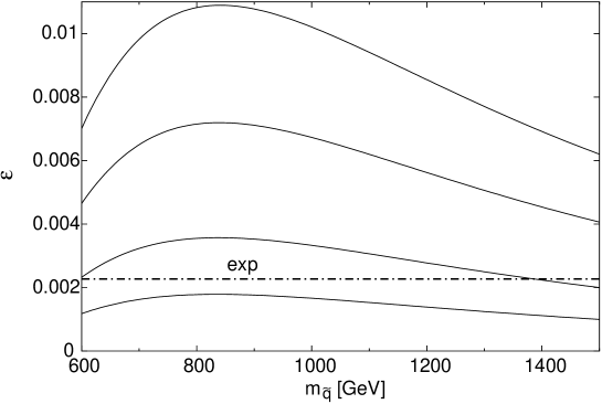
Figure 2: $\epsilon^{\rm SUSY}$ in the large angle MSW case for $M_{\nu_{R}}=5\times 10^{13}$, $1\times 10^{14}$, $2\times 10^{14}$ and $3\times 10^{14}\rm{GeV}$ from the below. We take $M_{2}=150~{}{\rm GeV}$, $a_{0}=0$, $\tan\beta=3$. The horizontal dash-dotted line corresponds to experimental value $\epsilon^{\rm exp}=2.271\times 10^{-3}$.

The same dependence in small angle MSW solution is shown in Fig 3, for $M_{\nu_{R}}=1\times 10^{14}$, $2\times 10^{14}$ and $3\times 10^{14}~{}{\rm GeV}$. Solid lines correspond to $s^{(L)}_{13}=0$ case. In this case $\epsilon^{\rm SUSY}$ is much smaller than that in large angle solution since $s^{(L)}_{12}$ is very small. However if $s^{(L)}_{13}$ is nonzero, the situation changes drastically. Dashed lines show results with $s^{(L)}_{13}=0.02$. In this case $\epsilon^{\rm SUSY}$ is enhanced and can be comparable to $\epsilon^{\rm exp}$ since $m_{\nu_{3}}$ is larger than $m_{\nu_{2}}$ by one order of magnitude and $s^{(L)}_{32}$ is also large. As $s^{(L)}_{13}$ gets close to the current upper limit of about 0.15, $\epsilon^{\rm SUSY}$ becomes much larger. Hence improvement of the limit on $s^{(L)}_{13}$ obtained by reactor experiments is very important to discuss CP violation in the kaon system in our model, especially for small angle case.

Figure 3: $\epsilon^{\rm SUSY}$ in the small angle MSW case, for $s^{(L)}_{13}=0$ (solid line) and $s^{(L)}_{13}=0.02$ (dashed line). In both cases, we choose $M_{\nu_{R}}=1\times 10^{14}$, $2\times 10^{14}$ and $3\times 10^{14}~{}{\rm GeV}$ from the below. We take $M_{2}=150~{}{\rm GeV}$, $a_{0}=0$ and $\tan\beta=3$. The horizontal dash-dotted line corresponds to experimental value $\epsilon^{\rm exp}=2.271\times 10^{-3}$.

It is important to consider the implication of the SUSY contribution to $\epsilon$ to the KM matrix since in the standard model, the $\epsilon$ parameter provides an important constraint on the $\rho$ vs. $\eta$ plane. In the standard model, the $\epsilon$ parameter is given as (see, for example, [31])

$$\epsilon^{\rm SM}\simeq C_{\epsilon}B_{K}A^{2}\lambda^{6}\eta\left[-\eta_{1}S_{0}(x_{c})+\eta_{3}S_{0}(x_{c},x_{t})+A^{2}\lambda^{4}(1-\rho)\eta_{2}S_{0}(x_{t})\right]e^{i\pi/4},$$ (3.13)

where $C_{\epsilon}=3.78\times 10^{4}$, $\eta_{1}$ $-$ $\eta_{3}$ are parameters for the QCD factors given by $\eta_{1}=1.38\pm 0.20$, $\eta_{2}=0.57\pm 0.01$, and $\eta_{3}=0.47\pm 0.04$, and Inami-Lim functions [32] $S_{0}(x_{c,t})$ and $S_{0}(x_{c},x_{t})$ are given by

$$S_{0}(x_{c,t}) = \frac{4x_{c,t}-11x_{c,t}^{2}+x_{c,t}^{3}}{4(1-x_{c,t})^{2}}-\frac{3x_{c,t}^{3}\log x_{c,t}}{2(1-x_{c,t})^{3}},$$ (3.14)

$$S_{0}(x_{c},x_{t}) = x_{c}\left[\log\left(\frac{x_{t}}{x_{c}}\right)-\frac{3x_{t}}{4(1-x_{t})}-\frac{3x_{t}^{2}\log x_{t}}{4(1-x_{t})^{2}}\right],$$ (3.15)

with $x_{c,t}=m_{c,t}^{2}/m_{W}^{2}$. In addition, we use $B_{K}=0.75-1.10$ [17]. Comparing Eq. (3.13) with the experimentally measured value of $\epsilon$, a constraint on the $\rho$ vs. $\eta$ plane is derived in the standard model.

If SUSY contribution to $\epsilon$ exists, such a constraint should be reconsidered. In particular, as we have seen, $\epsilon^{\rm SUSY}$ may be as large as the experimetally measured value of $\epsilon$, and hence the observed value of $\epsilon$ may have a significant amount of a contamination of $\epsilon^{\rm SUSY}$. Since the size of $\epsilon^{\rm SUSY}$ is model dependent and hence is unknown, we should disregard the constraint from the $\epsilon$ parameter. Of course, the $\rho$ vs. $\eta$ plane is still constrained by other quantities like $|[V_{\rm KM}]_{ub}/[V_{\rm KM}]_{cb}|$ and $\Delta m_{B_{d}}$, which are related to the parameters in the KM matrix as $|[V_{\rm KM}]_{ub}/[V_{\rm KM}]_{cb}|\simeq\lambda(\rho^{2}+\eta^{2})^{1/2}$, and

$$\Delta m_{B_{d}}\simeq\frac{G_{\rm F}^{2}}{6\pi^{2}}\eta_{B}m_{B_{d}}(F_{B_{d}}^{2}B_{B_{d}})m_{W}^{2}S_{0}(x_{t})A^{6}\lambda^{2}\left[(1-\rho)^{2}+\eta^{2}\right],$$ (3.16)

where $F_{B_{d}}\sqrt{B_{B_{d}}}=(200\pm 40)\ {\rm MeV}$, and $\eta_{B}=0.55\pm 0.01$ [31].

Importantly, the allowed region on the $\rho$ vs. $\eta$ plane changes as we exclude the constraint from $\epsilon$. Accordingly, possible size of the CP violation in the KM matrix, i.e., the $\eta$-parameter, changes.

To make a more quiantitative discussion, we derived constraints on the $\rho$ vs. $\eta$ plane comparing the standard model predictions on $\epsilon$, $|[V_{\rm KM}]_{ub}/[V_{\rm KM}]_{cb}|$ and $\Delta m_{B_{d}}$ with their experimental values. With and without the constraint from $\epsilon$, we found the upper and lower bounds on the $\eta$ parameter become

$$0.26\leq\eta\leq 0.48 : \mbox{with $\epsilon$},$$ (3.17)

$$0.17\leq\eta\leq 0.53 : \mbox{without $\epsilon$},$$ (3.18)

where we assumed flat distributions of the uncertainties in various parameters given above, and we adopted $A=0.834\pm 0.039$ [17]. As one can see, the upper and lower bounds on $\eta$ changes by about 10 % and 35 %, respectively, if the constraint from $\epsilon$ is not taken into account. This fact has important implications to future studies of CP violations using rare processes like $K_{L}\rightarrow\pi^{0}\nu\bar{\nu}$, as will be discussed in the following subsection.

3.2 $K_{L}\rightarrow\pi^{0}\nu\bar{\nu}$

In the future, we may have another interesting information of the CP violation via the rare process $K_{L}\rightarrow\pi^{0}\nu\bar{\nu}$. In the standard model, this process is mostly a signal of direct CP violation, and the amplitude for this mode is proportional to $\eta$. Most importantly, hadronic contribution to $K_{L}\rightarrow\pi^{0}\nu\bar{\nu}$ is small, and short distance effects of QCD are well under control [33]. Therefore, this mode is theoretically very clean. Although the branching ratio for this process is very small, we may have substantial number of $K_{L}\rightarrow\pi^{0}\nu\bar{\nu}$ event in future experiments [6], which may provide important test of the unitarity of the KM matrix. Due to Ref. [6], the $\eta$ parameter may be determined at 10 % accuracy.

This fact has an important implication to the search for the new physics. In the standard model, the $\eta$ parameter determined by $K_{L}\rightarrow\pi^{0}\nu\bar{\nu}$ should be consistent with that from other constraints, in particular, that from $\epsilon$. If the SUSY contribution to $\epsilon$ is sizable, however, this may not be realized. Indeed, as discussed in the previous subsection, the upper and lower bounds on $\eta$ may vary by about 10 % and 35 %, respectively, if the constraint from $\epsilon$ is not taken into account. Given the fact that $\eta$ may be determined with the accuracy of 10 % [6], measurement of $\eta$ in the experiment of $K_{L}\rightarrow\pi^{0}\nu\bar{\nu}$ gives an important constraint on $\rho$ vs. $\eta$ plane independetly with the measurement of $\epsilon$.

Of course, the Wilson coefficients for $K_{L}\rightarrow\pi^{0}\nu\bar{\nu}$ may be directly affected by the SUSY loops. Thus, we also calculated the SUSY correction to the $K_{L}\rightarrow\pi^{0}\nu\bar{\nu}$ process in our framework.

There are penguin and box diagrams in SUSY loop corrections which induce $K_{L}\rightarrow\pi^{0}\nu\bar{\nu}$. Effective operators are ${\cal Q}_{LL}^{\nu}\equiv(\bar{d}_{L}\gamma^{\mu}s_{L})(\bar{\nu}_{L}\gamma_{\nu}\nu_{L})$ and ${\cal Q}_{RL}^{\nu}\equiv(\bar{d}_{R}\gamma^{\mu}s_{R})(\bar{\nu}_{L}\gamma_{\nu}\nu_{L})$ with corresponding Wilson coefficients $C_{LL}^{\nu}$ and $C_{RL}^{\nu}$. SUSY contributions to Wilson coefficients are summarized in the Appendix B. For the process $K_{L}\rightarrow\pi^{0}\nu\bar{\nu}$, we found that the total SUSY contribution to the Wilson coefficients is a few % of the SM contribution, and that the SUSY contribution has distractive interference with the SM one in our model. As a result, it is challenging to see this deviation in the experiments.

For reasonable choices of parameters, the dominant SUSY contributions are from chargino and charged higgs penguin diagrams. Thus, the CP violating phase is controled by the phase in the KM matrix since the SUSY contribution is approximatelhy proportional to the 1-2 element of the left-handed squark mass matrix. On the contrary, effects of the GUT phases are tiny in $K_{L}\rightarrow\pi^{0}\nu\bar{\nu}$ because of the smalless of neutralino contribution which is, we found, mostly 0.1 % level. Since the SUSY contributions to this mode are quite small to be observed, useful information about the parameter $\eta$ is expected from $Br(K_{L}\rightarrow\pi^{0}\nu\bar{\nu})$ in our model.

3.3 $\epsilon^{\prime}/\epsilon$

In supersymmetric models, the parameter $\epsilon^{\prime}$ can be also modified due to the supersymmetric loop effects. In particular, in Ref. [34], it was pointed out that the SUSY contribution to $\epsilon^{\prime}/\epsilon$ may become much larger than the experimental value, $(\epsilon^{\prime}/\epsilon)^{\rm exp}=(19.3\pm 2.4)\times 10^{-4}$ [35], because of the significant modification of the $\Delta I=\frac{3}{2}$ amplitude contributing to $\epsilon^{\prime}/\epsilon$. As a result, in some parameter space, $\epsilon^{\prime}/\epsilon$ provides severer constraint on CP and flavor violations in the soft SUSY breaking parameters than the $\epsilon$ does, and hence one might worry if the SUSY contribution to $\epsilon^{\prime}/\epsilon$ is in a reasonable range in our framework. In this subsection, we discuss the SUSY contribution to $\epsilon^{\prime}/\epsilon$.

Before discussing the supersymmetric effect on $\epsilon^{\prime}/\epsilon$, let us first introduce several formulae necessary to evaluate $\epsilon^{\prime}/\epsilon$. The $\epsilon^{\prime}/\epsilon$ parameter is calculated once the Wilson coefficients for the $\Delta S=1$ effective Hamiltonian are given. The $\Delta S=1$ effective Hamiltonian is denoted as

$${\cal H}_{\rm eff}^{(\Delta S=1)} = \sum_{i}\left(C_{L,i}^{(\Delta S=1)}{\cal Q}_{L,i}^{(\Delta S=1)}+C_{R,i}^{(\Delta S=1)}{\cal Q}_{R,i}^{(\Delta S=1)}\right),$$ (3.19)

where $C_{i}$ are Wilson coefficients, and

$${\cal Q}_{L,3}^{(\Delta S=1)} = 4(\bar{s}_{\alpha}\gamma_{\mu}P_{L}d_{\alpha})\sum_{q}(\bar{q}_{\beta}\gamma_{\mu}P_{L}q_{\beta}),$$ (3.20)

$${\cal Q}_{L,4}^{(\Delta S=1)} = 4(\bar{s}_{\alpha}\gamma_{\mu}P_{L}d_{\beta})\sum_{q}(\bar{q}_{\beta}\gamma_{\mu}P_{L}q_{\alpha}),$$ (3.21)

$${\cal Q}_{L,5}^{(\Delta S=1)} = 4(\bar{s}_{\alpha}\gamma_{\mu}P_{L}d_{\alpha})\sum_{q}(\bar{q}_{\beta}\gamma_{\mu}P_{R}q_{\beta}),$$ (3.22)

$${\cal Q}_{L,6}^{(\Delta S=1)} = 4(\bar{s}_{\alpha}\gamma_{\mu}P_{L}d_{\beta})\sum_{q}(\bar{q}_{\beta}\gamma_{\mu}P_{R}q_{\alpha}),$$ (3.23)

$${\cal Q}_{L,7}^{(\Delta S=1)} = 4(\bar{s}_{\alpha}\gamma_{\mu}P_{L}d_{\alpha})\sum_{q}e_{q}(\bar{q}_{\beta}\gamma_{\mu}P_{R}q_{\beta}),$$ (3.24)

$${\cal Q}_{L,8}^{(\Delta S=1)} = 4(\bar{s}_{\alpha}\gamma_{\mu}P_{L}d_{\beta})\sum_{q}e_{q}(\bar{q}_{\beta}\gamma_{\mu}P_{R}q_{\beta}),$$ (3.25)

$${\cal Q}_{L,9}^{(\Delta S=1)} = 4(\bar{s}_{\alpha}\gamma_{\mu}P_{L}d_{\alpha})\sum_{q}e_{q}(\bar{q}_{\beta}\gamma_{\mu}P_{L}q_{\beta}),$$ (3.26)

$${\cal Q}_{L,10}^{(\Delta S=1)} = 4(\bar{s}_{\alpha}\gamma_{\mu}P_{L}d_{\beta})\sum_{q}e_{q}(\bar{q}_{\beta}\gamma_{\mu}P_{L}q_{\alpha}),$$ (3.27)

with $P_{L/R}=\frac{1}{2}(1\mp\gamma_{5})$, $\alpha$ and $\beta$ being the color indices, $e_{q}$ denoting the quark electric charge, and ${\cal Q}_{R,i}^{(\Delta S=1)}\equiv{\cal Q}_{L,i}^{(\Delta S=1)}|_{L\leftrightarrow R}$. Based on the structure of the operators, we call ${\cal Q}_{L,i}^{(\Delta S=1)}$ with $i=3$, 4, 9 and 10 (${\cal Q}_{R,i}^{(\Delta S=1)}$ with $i=3$, 4, 9 and 10) as $LL$-type ($RR$-type) operators while others as $LR$- or $RL$-type operators.

In the standard model, the gluon-penguin diagram generates the operators ${\cal Q}_{L,i}^{(\Delta S=1)}$ with $i=3-6$, and hence their Wilson coefficients are of $O(\alpha_{\rm W}\alpha_{\rm s})$ where $\alpha_{\rm W}$ indicates the coupling constants for the electroweak interaction. On the contrary, the operators ${\cal Q}_{L,i}^{(\Delta S=1)}$ with $i=7-10$ are only from the electroweak processes and the corresponding Wilson coefficients are of $O(\alpha_{\rm W}^{2})$. Although the Wilson coefficients contributing to the $\Delta I=\frac{3}{2}$ amplitude are smaller than those contributing to the $\Delta I=\frac{1}{2}$ one, both amplitudes are significant since the $\Delta I=\frac{3}{2}$ contribution has extra enhancement factor.

From the effective Hamiltonian given in Eq. (3.19), $\epsilon^{\prime}/\epsilon$ is given by (see, for example, [31])

$$\frac{\epsilon^{\prime}}{\epsilon} = \frac{G_{\rm F}\omega}{2|\epsilon|{\rm Re}A_{0}}\sum_{i}{\rm Im}C_{L,i}^{(\Delta S=1)}\left[(1-\Omega_{\eta\eta^{\prime}})\langle(\pi\pi)_{I=0}|{\cal Q}_{L,i}^{(\Delta S=1)}|K\rangle-\frac{1}{\omega}\langle(\pi\pi)_{I=2}|{\cal Q}_{L,i}^{(\Delta S=1)}|K\rangle\right]$$ (3.28)

$$+(L\rightarrow R),$$

where $|(\pi\pi)_{I}\rangle$ denotes the two-pion state with isospin $I$, and

$$\omega\equiv\frac{{\rm Re}A_{2}}{{\rm Re}A_{0}},$$ (3.29)

with

$$A_{0}\equiv\langle(\pi\pi)_{I=0}|{\cal H}_{\rm eff}|K\rangle,~{}~{}~{}A_{2}\equiv\langle(\pi\pi)_{I=2}|{\cal H}_{\rm eff}|K\rangle.$$ (3.30)

Numerically, $\omega\simeq 0.045$. In addition, $\Omega_{\eta\eta^{\prime}}$ is from the isospin breaking in the quark masses, and numerically we use $\Omega_{\eta\eta^{\prime}}=0.25$ [31]. Since $\omega$ is a small number, the $\Delta I=\frac{3}{2}$ contribution in Eq. (3.28), which is proportional to $\omega^{-1}$, is enhanced relative to the $\Delta I=\frac{1}{2}$ contribution.

Now, let us consider the supersymmetric contribution to $\epsilon^{\prime}/\epsilon$. In MSSM, the Wilson coefficients for the $\Delta S=1$ effective Lagrangian are modified by integrating out supersymmetric particles. (Formulae for the SUSY contribution to the Wilson coefficients are given in Appendix C.) With the SUSY contribution to the Wilson Coefficients given at the electroweak scale, we can calculate $\epsilon^{\prime}/\epsilon$ using the same prescription as the SM case.

One important observation is that, in MSSM, $\Delta I=\frac{3}{2}$ contribution can be largely enhanced relative to the standard model case [34]. This is because the $\Delta I=\frac{3}{2}$ contribution is, as mentioned before, of $O(\alpha_{\rm W}^{2})$ in the standard model while it can be of $O(\alpha_{\rm s}^{2})$ in MSSM if the mass matrix of the down-type squarks has non-vanishing 1-2 element. Combining the fact that $\Delta I=\frac{3}{2}$ contribution is enhanced by the factor $\omega^{-1}\simeq 22$, the SUSY contribution to the $\epsilon^{\prime}/\epsilon$ parameter can be order of magnitude larger than the experimental value. Thus, in some case, constraint on the CP and flavor violating parameters in MSSM from $\epsilon^{\prime}/\epsilon$ becomes severer than that from $\epsilon$.

As we will see below, the SUSY contribution to $\epsilon^{\prime}/\epsilon$ is relatively small in our framework. Before showing the numerical results, let us explain how the the smallness of $\epsilon^{\prime}/\epsilon$ is understood in our framework compared to the result given in Ref. [34].

As a first step, let us briefly review how the large SUSY contribution is realized in Ref. [34]. The most important enhancement is for the the $LR$-type $\Delta I=\frac{3}{2}$ amplitude by the factor of $\sim\alpha_{\rm s}^{2}/\alpha_{\rm W}^{2}$ relative to the SM contributions. The same enhancement also exists for the $LL$- and $RR$-type operators. However, in taking the relevant matrix elements of the $LR$-type operators, there is a chirality-enhancement factor proportional to $m_{K}^{2}/m_{s}^{2}\sim 10$, and hence the $LR$-type operators are more important than the $LL$- and $RR$ ones.

Since the $\Delta I=\frac{3}{2}$ amplitude is an isospin-breaking effect, a mass difference between the up- and down-squark masses is necessary. For the right-handed up- and down-squarks, significant mass splitting is realized if the SUSY breaking mass parameters for them take different values. On the contrary, the left-handed ones are both from the SU(2)_L-doublet. As a result, their mass splitting is only from the electroweak symmetry breaking effect (i.e., vacuum expectation values of the Higgs bosons), and the mass splitting between left-handed squarks is too small to generate significant contribution to the isospin-breaking amplitude. Thus, in order to generate $LR$-type operators, sizable 1-2 element of the left-handed down-type squark mass matrix is necessary. In summary, the condition for the large SUSY contribution to $\epsilon^{\prime}/\epsilon$ is (i) mass splitting of between $\tilde{u}_{R}$ and $\tilde{d}_{R}$, and (ii) non-vanishing imaginary part of $[m_{\tilde{d}_{L}}^{2}]_{12}$. Combining all of these effects, the SUSY contribution to $\epsilon^{\prime}/\epsilon$ can be as large as $10^{-2}$ when ${\rm Im}([m_{\tilde{d}_{L}}^{2}]_{12}/m^{2}_{\tilde{d}})\sim 10^{-2}$.

Now, we turn to our case. In our framework, large off-diagonal elements are generated for the right-handed down-type squark mass matrix since they are related to the neutrino Yukawa interactions. Since sizable mass splitting between up- and down-type squarks is possible only for the right-handed sector, only the $RR$-type contribution is modified for the $\Delta I=\frac{3}{2}$ process, and hence the chirality enhancement is not significant for $\Delta I=\frac{3}{2}$ process. In addition, if we take the universal boundary condition for the squark masses, mass splitting between $\tilde{u}_{R}$ and $\tilde{d}_{R}$ is fairly small. As a result, correction to the $\Delta I=\frac{3}{2}$ amplitude becomes small.

To make more quantitative discussion, we calculate the SUSY contributions to the $\Delta I=\frac{1}{2}$ and $\Delta I=\frac{3}{2}$ part of $\epsilon^{\prime}/\epsilon$. In our analysis, we followed the prescription given in Ref. [31] to calculate the SUSY contribution to $\epsilon^{\prime}/\epsilon$. We first calculate the SUSY contribution to the Wilson coefficients at the electroweak scale. Then, we run them down to the charm quark mass scale using the relevant RGEs and took the matrix elements. The resultant SUSY contribution is linear in the Wilson coefficients, and numerically we found

$$(\epsilon^{\prime}/\epsilon)^{\rm SUSY}=\sum_{i}N_{i}{\rm Im}\left[\tilde{C}_{L,i}^{(\Delta S=1)}(\mu=m_{W})+\tilde{C}_{R,i}^{(\Delta S=1)}(\mu=m_{W})\right],$$ (3.31)

where $\tilde{C}_{L,i}^{(\Delta S=1)}$ and $\tilde{C}_{R,i}^{(\Delta S=1)}$ are SUSY contribution to the corresponding Wilson coefficients, and the numerical values for $N_{i}$ are given in Table 1.

$m_{s}$	0.11 GeV	0.13 GeV	0.15 GeV
$N_{3}$	$6.64\times 10^{4}$	$8.92\times 10^{5}$	$1.42\times 10^{6}$
$N_{4}$	$-9.98\times 10^{6}$	$-9.01\times 10^{6}$	$-8.39\times 10^{6}$
$N_{5}$	$1.44\times 10^{7}$	$1.07\times 10^{7}$	$8.29\times 10^{6}$
$N_{6}$	$4.30\times 10^{7}$	$3.22\times 10^{7}$	$2.52\times 10^{7}$
$N_{7}$	$8.28\times 10^{8}$	$5.97\times 10^{8}$	$4.49\times 10^{8}$
$N_{8}$	$2.60\times 10^{9}$	$1.89\times 10^{9}$	$1.43\times 10^{9}$
$N_{9}$	$9.08\times 10^{6}$	$1.10\times 10^{7}$	$1.23\times 10^{7}$
$N_{10}$	$2.32\times 10^{6}$	$3.46\times 10^{6}$	$4.19\times 10^{6}$

Table 1: Coefficients $N_{i}$ in units of GeV² for the fitting formula of the $\epsilon^{\prime}/\epsilon$ parameter. We use the bag parameters given in Ref. [31], and $m_{s}=0.11$, 0.13, and 0.15 GeV.

Figure 4: Contours of constant $R_{1/2}$ in units of $10^{-2}$, which is $(\epsilon^{\prime}/\epsilon)^{\rm SUSY}_{\Delta I=1/2}$ normalized by the standard model contribution. Here, we consider the large angle MSW case and take $M_{\nu_{R}}=3\times 10^{14}\ {\rm GeV}$, $\tan\beta=3$, and $m_{s}=0.13$ GeV.

Figure 5: Contours of constant $R_{3/2}$ in units of $10^{-2}$, which is $(\epsilon^{\prime}/\epsilon)^{\rm SUSY}_{\Delta I=3/2}$ normalized by the standard model contribution. Here, we consider the large angle MSW case and take $M_{\nu_{R}}=3\times 10^{14}\ {\rm GeV}$, $\tan\beta=3$, and $m_{s}=0.13$ GeV.

First, we present the SUSY contribution to the $\Delta I=\frac{1}{2}$ and $\Delta I=\frac{3}{2}$ part of $\epsilon^{\prime}/\epsilon$ normalized by the standard model ones:

$$R_{1/2}\equiv\frac{(\epsilon^{\prime}/\epsilon)^{\rm SUSY}_{\Delta I=1/2}}{(\epsilon^{\prime}/\epsilon)^{\rm SM}_{\Delta I=1/2}},~{}~{}~{}R_{3/2}\equiv\frac{(\epsilon^{\prime}/\epsilon)^{\rm SUSY}_{\Delta I=3/2}}{(\epsilon^{\prime}/\epsilon)^{\rm SM}_{\Delta I=3/2}}.$$ (3.32)

In Figs. 5 and 5, we plot contours of constant $R_{1/2}$ and $R_{3/2}$ on $m_{\tilde{q}}$ vs. $\varphi^{(L)}_{1}-\varphi^{(L)}_{2}$ plane for the case of the large angle MSW. Here, we take $M_{\nu_{R}}=3\times 10^{14}\ {\rm GeV}$, and $\tan\beta=3$. As one can see, the SUSY contribution is at most a few % of the standard model contribution for the $\Delta I=\frac{1}{2}$ part, and $\sim 10\ \%$ for the $\Delta I=\frac{3}{2}$ one. It is notable that, in our simple analysis, universal scalar mass is assumed as a boundary condition. Consequently, mass splitting between the right-handed up- and down-type squarks becomes small since the masses of these squarks are mostly determined by the boundary condition and the RG effect due to the gluino loop below the GUT scale which are universal in this case. As a result, masses of the right-handed up- and down-type squarks are quite degenerate, and this fact gives another suppression factor for the $\Delta I=\frac{3}{2}$ contribution. Since the contributions to the $\Delta I=\frac{1}{2}$ and $\Delta I=\frac{3}{2}$ amplitudes are both small, the SUSY contribution to the $\epsilon^{\prime}/\epsilon$ parameter is also at most a few % level in our framework.

4 Conclusions and Discussion

In this paper, we discussed CP violations in the supersymmetric SU(5) model with right-handed neutrinos. In this class of model, off-diagonal elements of the right-handed down-type squarks are generated via the RG effect even if they vanish at the cut-off scale (i.e., in our case, the reduced Planck scale). In general, such off-diagonal elements contain CP violating phases and they can be extra sources of the CP violations in the low-energy processes. In particular, it was emphasized that such phases can be related to phases in the unified theories, which are not related to the parameters in the standard model.

We paid particular attentions to the CP violations in the kaon system. Most importantly, we have seen that the $\epsilon$ parameter can be severely affected by the SUSY contribution; even with a relatively heavy squark mass of $\sim 1\ {\rm TeV}$, the SUSY contribution to $\epsilon$ can be as large as the experimentally measured value if the Majorana mass for the right-handed neutrinos is as large as $\sim 10^{14}\ {\rm GeV}$. Of course, the SUSY contribution to $\epsilon$ strongly depends on the phases in the off-diagonal elements of the squark mass matrix. As we have seen, the phases in these parameters can be naturally large due to the phases in the GUT model.

We have also calculated the SUSY contribution to $Br(K_{L}\rightarrow\pi^{0}\nu\bar{\nu})$ and $\epsilon^{\prime}/\epsilon$. Unfortunately, however, the SUSY contributions to these quantities are relatively small. In our framework, SUSY contribution to $Br(K_{L}\rightarrow\pi^{0}\nu\bar{\nu})$ is a few %, and the SUSY contribution to $\epsilon^{\prime}/\epsilon$ is also a few % level of the standard model one.

Thus, in our framework, the SUSY contribution is the most important for the $\epsilon$ parameter. This fact has an important implication to the future test of the unitarity of the KM matrix, since $\epsilon$ provides one of the important information of the magnitude of the CP violation in the KM matrix in the standard model. In the standard model, the so-called $\rho$ vs. $\eta$ plane was constrained so that the standard-model prediction of the $\epsilon$ parameter agrees with observed one. If the SUSY contribution to $\epsilon$ is sizable, however, $\epsilon$ cannot be used to constrain the $\rho$ vs. $\eta$ plane, which may change the bounds on $\rho$ and $\eta$. We have seen that the upper and lower bounds on the $\eta$ parameter changes by about 10 % and 35 %, respectively, if we discard the constraint from $\eta$. The deviation from the standard-model prediction on $\eta$ may be tested by future experiments. In particular, the measurements of $\phi_{1}$ and $Br(K_{L}\rightarrow\pi^{0}\nu\bar{\nu})$ will provide an interesting test of the value of $\eta$. Notice that there are still sizable uncertainties in the theoretical calculation of the $\epsilon$ parameter, in particular from the bag parameter in taking the hadronic matrix elements and from the Wolfenstein’s $A$-parameter in the KM matrix. Thus, reduction of the uncertainties in these quantities will be very important to find a signal of the SUSY loop using the $\epsilon$ parameter.

Note Added: In finalizing this paper, we found a paper by S. Baek et al. [37] which has some overlap with our analysis. In particular, in [37], authors paid special attention to non-minimal contribution to the Yukawa matrices at the GUT scale in order to realize a realistic unification of the down-type and charged-lepton Yukawa matrices.

Acknowledgment: One of the authors (TM) would like to thank H. Murayama for useful conversations. The work of Y.K. is supported by the Japan Society for the Promotion of Science. The work of T.M. is supported by the Grant-in-aid from the Ministry of Education, Culture, Sports, Science and Technology, Japan, No.12047201.

Appendix A Interaction Lagrangian

In this section, we show the interaction Lagrangian used in this paper. Relevant terms in our calculation are the vertices for charginos, neutralinos and gluinos with squarks and quarks. At first, we begin relation between gauge and mass eigenstates and mixing matrix, which make mass matrix diagonalized.

The mass and gauge eigenstates for squarks are denoted with $\tilde{q_{A}}$ ($A=1,\cdots,6$), $\tilde{q_{i}}_{L/R}$ ($i=1,2,3$, label for generation), respectively. Then the relations between gauge and mass eigenstates are given by:

$$\tilde{q}_{iL}=[U(\tilde{q})]_{iA}\tilde{q}_{A},~{}~{}~{}\tilde{q}_{iR} = [U(\tilde{q})]_{(i+3)A}\tilde{q}_{A},$$ (A.1)

where $U(\tilde{q})$ is a $6\times 6$ unitary matrix which diagonalize squark mass matrix ${\cal M}^{2}_{\tilde{q}}$,

$$[U^{\dagger}(\tilde{q}){\cal M}^{2}_{\tilde{q}}U(\tilde{q})]_{AB}=m_{\tilde{q}_{A}}^{2}\delta_{AB}.$$ (A.2)

Relation between gauge and mass eigenstate for charginos and neutralinos are given by

$$\left[\begin{array}[]{c}\tilde{W}_{L}^{-}\\ \tilde{H}_{1L}^{-}\end{array}\right]_{i} = [U(\tilde{\chi}^{-}_{L})]_{iX}\tilde{\chi}^{-}_{X\,L},$$ (A.5)

$$\left[\begin{array}[]{c}\tilde{W}_{R}^{-}\\ \tilde{H}_{2R}^{-}\end{array}\right]_{i} = [U(\tilde{\chi}^{-}_{R})]_{iX}\tilde{\chi}^{-}_{X\,R},$$ (A.8)

$$\left[\begin{array}[]{c}\tilde{B}_{L}\\ \tilde{W}_{L}^{3}\\ \tilde{H}_{1L}^{0}\\ \tilde{H}_{2L}^{0}\\ \end{array}\right]_{i} = [U(\tilde{\chi}^{0})]_{iX}\tilde{\chi}^{0}_{X\,L},$$ (A.13)

where $U(\tilde{\chi}^{-}_{L/R})$ and $U(\tilde{\chi}^{0})$ are $2\times 2$ and $4\times 4$ unitary matrices which diagonalize mass matrix for charginos and neutralinos, respectively. Diagonalization of mass matrices gives masses of charginos $m_{\tilde{\chi}^{-}_{X}}$ and neutralinos $m_{\tilde{\chi}^{0}_{X}}$ ,

$$[U^{\dagger}(\tilde{\chi}^{-}_{R}){\cal M}_{\tilde{\chi}^{-}}U(\tilde{\chi}^{-}_{L})]_{XY}=m_{\tilde{\chi}^{-}_{X}}\delta_{XY},~{}~{}~{}[U^{\dagger}(\tilde{\chi}^{0}){\cal M}_{\tilde{\chi}^{0}}U(\tilde{\chi}^{0})]_{XY}=m_{\tilde{\chi}^{0}_{X}}\delta_{XY},$$ (A.14)

For quarks, we chose the basis in which the mass eigenstates $(u,d)$ and gauge eigenstates $(u^{\prime},d^{\prime})$ are related as $d^{\prime}_{L}=d_{L}$, $u^{\prime}_{L}=V_{\rm{KM}}~{}u_{L}$, $u^{\prime}_{R}=u_{R}$ and $d^{\prime}_{R}=d_{R}$.

The interaction Lagrangian for chargino-quark-squark couplings are given by

$$L_{{\tilde{\chi}^{-}}d\tilde{u}} = \bar{\tilde{\chi}}^{-}_{X}\left(C_{dAX}^{L}P_{L}+C_{dAX}^{R}P_{R}\right)d\tilde{u}_{A}^{\ast}$$ (A.15)

$$+u^{T}(-C^{\dagger})\left(C_{uAX}^{L}P_{L}+C_{uAX}^{R}P_{R}\right)\tilde{\chi}^{-}_{X}\tilde{d}_{A}^{\ast}+h.c.,$$

where $C$ is the charge conjugation matrix, $P_{L/R}=\frac{1}{2}\left(1\mp\gamma_{5}\right)$, and $u$ and $d$ denote up-type ($u,c,t$) and down-type ($d,s,b$) quarks, respectively. $C_{qAX}^{L,R}$ are given by

$$C_{dAX}^{L} = -g_{2}[U^{\ast}(\tilde{\chi}^{-}_{R})]_{1X}[U^{\ast}(\tilde{u})]_{dA}+[U^{\ast}(\tilde{\chi}^{-}_{R})]_{2X}\sum_{j=1}^{3}[U^{\ast}(\tilde{u})]_{(3+j)A}[\hat{Y}_{U}V_{\rm KM}]_{jd},$$ (A.16)

$$C_{dAX}^{R} = -[U^{\ast}(\tilde{\chi}^{-}_{L})]_{2X}[U^{\ast}(\tilde{u})]_{dA}[\hat{Y}_{D}]_{d},$$ (A.17)

$$C_{uAX}^{L} = -g_{2}[U(\tilde{\chi}^{-}_{L})]_{1X}\sum_{j=1}^{3}[U^{\ast}(\tilde{d})]_{jA}[V_{\rm KM}^{\ast}]_{uj}$$ (A.18)

$$-[U(\tilde{\chi}^{-}_{L})]_{2X}\sum_{j=1}^{3}[U^{\ast}(\tilde{d})]_{(3+j)A}[\hat{Y}_{D}\,V_{KM}^{\dagger}]_{ju},$$

$$C_{uAX}^{R} = [U(\tilde{\chi}^{-}_{R})]_{2X}\sum_{j=1}^{3}[U^{\ast}(\tilde{d})]_{jA}[V_{\rm KM}^{\dagger}\,\hat{Y}_{U}^{\dagger}]_{ju},$$ (A.19)

where $g_{2}$ is the gauge coupling constant of SU(2)_L, and $u,d=(1,2,3)$ for $(u,c,t)$ and $(d,s,b)$, respectively.

Neutralino-quark-squark coupling couplings are given by

$${\cal L}_{{\tilde{\chi}^{0}}d\tilde{d}} = \bar{\tilde{\chi}}^{0}_{X}\left(N_{dAX}^{L}P_{L}+N_{iAX}^{R}P_{R}\right)d\tilde{d}_{A}^{\ast}$$ (A.20)

$$+\bar{\tilde{\chi}}^{0}_{X}\left(N_{uAX}^{L}P_{L}+N_{uAX}^{R}P_{R}\right)u\tilde{u}_{A}^{\ast}+h.c.,$$

where

$$N_{dAX}^{L} = \left(-\frac{\sqrt{2}g_{1}}{6}[U(\tilde{\chi}^{0})]_{1X}+\frac{\sqrt{2}g_{2}}{2}[U(\tilde{\chi}^{0})]_{2X}\right)[U^{\ast}(\tilde{d})]_{dA}$$ (A.21)

$$+[U(\tilde{\chi}^{0})]_{3X}[U^{\ast}(\tilde{d})]_{(d+3)A}[\hat{Y}_{D}]_{d},$$

$$N_{dAX}^{R} = -\frac{\sqrt{2}g_{1}}{3}[U^{\ast}(\tilde{\chi}^{0})]_{1X}[U^{\ast}(\tilde{d})]_{(d+3)A}+[U^{\ast}(\tilde{\chi}^{0})]_{3X}[U^{\ast}(\tilde{d})]_{dA}[\hat{Y}_{D}^{\dagger}]_{d},$$ (A.22)

$$N_{uAX}^{L} = \left(-\frac{\sqrt{2}g_{1}}{6}[U(\tilde{\chi}^{0})]_{1X}-\frac{\sqrt{2}g_{2}}{2}[U(\tilde{\chi}^{0})]_{2X}\right)[U^{\ast}(\tilde{u})]_{uA}$$ (A.23)

$$-[U(\tilde{\chi}^{0})]_{4X}\sum_{j=1}^{3}[U^{\ast}(\tilde{u})]_{(j+3)A}[\hat{Y}_{U}V_{\rm KM}]_{ju},$$

$$N_{uAX}^{R} = \frac{2\sqrt{2}g_{1}}{3}[U^{\ast}(\tilde{\chi}^{0})]_{1X}[U^{\ast}(\tilde{u})]_{(u+3)A}$$ (A.24)

$$-[U^{\ast}(\tilde{\chi}^{0})]_{4X}\sum_{j=1}^{3}[U^{\ast}(\tilde{u})]_{jA}[V_{\rm KM}^{\dagger}\hat{Y}_{U}^{\dagger}]_{ju},$$

with $g_{1}$ being the gauge coupling constant of U(1)_Y.

The interaction Lagrangian for gluino-quark-squark coupling is given by

$$L_{\tilde{G}q\tilde{q}} = \tilde{d}_{A}^{\ast}\bar{\tilde{G}^{a}}T^{a}\left(G_{dA}^{L}P_{L}+G_{dA}^{R}P_{R}\right)d$$ (A.25)

$$+\tilde{u}_{A}^{\ast}\bar{\tilde{G}^{a}}T^{a}\left(G_{uA}^{L}P_{L}+G_{uA}^{R}P_{R}\right)u+h.c.,$$

where

$$G_{dA}^{L} = -\sqrt{2}g_{s}[U^{\ast}(\tilde{d})]_{iA},$$ (A.26)

$$G_{dA}^{R} = \sqrt{2}g_{s}[U^{\ast}(\tilde{d})]_{(i+3)A},$$ (A.27)

$$G_{uA}^{L} = -\sqrt{2}g_{s}\sum_{j=1}^{3}[U^{\ast}(\tilde{u})]_{jA}[V_{\rm KM}^{\ast}]_{ju},$$ (A.28)

$$G_{uA}^{R} = \sqrt{2}g_{s}[U^{\ast}(\tilde{u})]_{(u+3)A},$$ (A.29)

with $g_{s}$ being the gauge coupling constant of SU(3)_C. Here we take soft-breaking mass parameter of gauginos as real positive.

Appendix B SUSY Contribution to $K_{L}\rightarrow\pi^{0}\nu\bar{\nu}$

In this appendix, we show the SUSY contribution to the Wilson coefficient of effective operators for $K_{L}\rightarrow\pi^{0}\nu\bar{\nu}$.

There are sets of SUSY loop diagrams in which charged-Higgs, charginos and neutralinos are exchanged, which induce effective operators

$${\cal Q}_{LL}^{\nu}\equiv(\bar{d}\gamma^{\mu}P_{L}s)(\bar{\nu}\gamma^{\mu}P_{L}\nu),~{}~{}~{}{\cal Q}_{RL}^{\nu}\equiv(\bar{d}\gamma^{\mu}P_{R}s)(\bar{\nu}\gamma^{\mu}P_{L}\nu).$$ (B.1)

The Wilson coefficients of corresponding operators are referred to $C_{LL}^{\nu}$ and $C_{RL}^{\nu}$, respectively. The effective Hamiltonian is given by ${\cal H}_{\rm eff}=(C_{LL}^{ZP,\nu}+C_{LL}^{{\rm Box},\nu}){\cal Q}_{LL}^{\nu}+(C_{RL}^{ZP,\nu}+C_{RL}^{{\rm Box},\nu}){\cal Q}_{RL}^{\nu}$.

In the following, each SUSY contribution of charged-Higgs, charginos and neutralinos are separately shown for $Z$-penguin diagrams,

$$\tilde{C}_{LL}^{ZP,\nu}|^{H^{-}} = \frac{g_{Z}^{2}}{2M_{Z}^{2}}m_{u}^{2}\left(T^{3}_{u_{R}}-T^{3}_{u_{L}}\right){H^{L}_{ud}}^{\ast}H^{L}_{us}I^{0}_{3}\left(m_{u}^{2},m_{u}^{2},m_{H^{-}}^{2}\right)$$ (B.2)

$$\tilde{C}_{LL}^{ZP,\nu}|^{\tilde{\chi}^{-}} = \frac{g_{Z}^{2}}{8M_{Z}^{2}}C^{L\ast}_{dAX}C^{L}_{sBY}$$ (B.3)

$$\times\Bigg{\{}\delta_{XY}\left[\sum_{j=1}^{3}[U^{\ast}(\tilde{u})]_{jA}[U(\tilde{u})]_{jB}-\delta_{AB}\left(1+2T^{3}_{d_{L}}\right)\right]\,I^{1}_{3}(m_{\tilde{\chi}_{X}^{-}}^{2},m_{\tilde{u}_{A}}^{2},m_{\tilde{u}_{B}}^{2})$$

$$+\delta_{AB}\Bigg{[}\,2m_{\tilde{\chi}_{X}^{-}}m_{\tilde{\chi}_{Y}^{-}}[U^{\ast}(\tilde{\chi}^{-}_{L})]_{1X}[U(\tilde{\chi}^{-}_{L})]_{1Y}\,I^{0}_{3}(m_{\tilde{\chi}_{X}^{-}}^{2},m_{\tilde{\chi}_{Y}^{-}}^{2},m_{\tilde{u}_{A}}^{2})$$

$$-[U^{\ast}(\tilde{\chi}^{-}_{R})]_{1X}[U(\tilde{\chi}^{-}_{R})]_{1Y}\,I^{1}_{3}(m_{\tilde{\chi}_{X}^{-}}^{2},m_{\tilde{\chi}_{Y}^{-}}^{2},m_{\tilde{u}_{A}}^{2})\Bigg{]}\Bigg{\}},$$

$$\tilde{C}_{LL}^{ZP,\nu}|^{\tilde{\chi}^{0}} = \frac{g_{Z}^{2}}{8M_{Z}^{2}}N^{L\ast}_{dAX}N^{L}_{sBY}$$

$$\times\Bigg{\{}\delta_{XY}\left[-\sum_{j=1}^{3}[U^{\ast}(\tilde{u})]_{jA}[U(\tilde{u})]_{jB}-2T^{3}_{d_{L}}\delta_{AB}\right]\,I^{1}_{3}(m_{\tilde{\chi}_{X}^{0}}^{2},m_{\tilde{d}_{A}}^{2},m_{\tilde{d}_{B}}^{2})$$

$$+\delta_{AB}\left[\,-2m_{\tilde{\chi}_{X}^{0}}m_{\tilde{\chi}_{Y}^{0}}O_{L}^{XY}\,I^{0}_{3}(m_{\tilde{\chi}_{X}^{-}}^{2},m_{\tilde{\chi}_{Y}^{-}}^{2},m_{\tilde{d}_{A}}^{2})+O_{R}^{XY}\,I^{1}_{3}(m_{\tilde{\chi}_{X}^{0}}^{2},m_{\tilde{\chi}_{Y}^{0}}^{2},m_{\tilde{d}_{A}}^{2})\right]\Bigg{\}},$$

with $g_{Z}=\sqrt{g_{1}^{2}+g_{2}^{2}}$ and

$${H^{L}_{ud}} = \frac{g_{2}\cot\beta\,m_{u}}{\sqrt{2}M_{W}}\left[V_{\rm KM}\right]_{ud},$$ (B.5)

$${H^{R}_{ud}} = \frac{g_{2}\tan\beta\,m_{d}}{\sqrt{2}M_{W}}[V_{\rm KM}]_{ud},$$ (B.6)

$$O_{L}^{XY} = [U^{\ast}(\tilde{\chi}^{0})]_{3X}[U(\tilde{\chi}^{0})]_{3Y}-[U^{\ast}(\tilde{\chi}^{0})]_{4X}[U(\tilde{\chi}^{0})]_{4Y},$$ (B.7)

$$O_{R}^{XY} = -O_{L}^{\ast XY}.$$ (B.8)

Here $T^{3}_{u_{R}}=T^{3}_{d_{R}}=0,\ T^{3}_{u_{L}}=-T^{3}_{d_{L}}=1/2$. $\tilde{C}_{RL}^{ZP,\nu}$ is obtained by interchanging $R$ with $L$, $\tilde{C}_{RL}^{ZP,\nu}=\tilde{C}_{LL}^{ZP,\nu}|_{L\leftrightarrow R}$.

The contributions from box-diagrams are given by

$$\tilde{C}_{LL}^{{\rm Box},\nu}|^{\tilde{\chi}^{-}} = -\frac{1}{2}m_{\tilde{\chi}_{X}^{-}}m_{\tilde{\chi}_{Y}^{-}}C^{L\ast}_{dAX}C^{L}_{sAY}C^{L\ast}_{\nu BX}C^{L}_{\nu BY}I^{0}_{4}(m_{\tilde{\chi}_{X}^{-}}^{2},m_{\tilde{\chi}_{Y}^{-}}^{2},m_{\tilde{u}_{A}}^{2},m_{\tilde{l}_{B}}^{2}),$$ (B.9)

$$\tilde{C}_{RL}^{{\rm Box},\nu}|^{\tilde{\chi}^{-}} = \frac{1}{4}C^{R\ast}_{dAX}C^{R}_{sAY}C^{L\ast}_{\nu BX}C^{L}_{\nu BY}I^{1}_{4}(m_{\tilde{\chi}_{X}^{-}}^{2},m_{\tilde{\chi}_{Y}^{-}}^{2},m_{\tilde{u}_{A}}^{2},m_{\tilde{l}_{B}}^{2}),$$ (B.10)

$$\tilde{C}_{LL}^{{\rm Box},\nu}|^{\tilde{\chi}^{0}} = -\frac{1}{4}N^{L\ast}_{\nu BX}N^{L}_{\nu BY}\left[\,2N^{L\ast}_{dAX}N^{L}_{sAY}m_{\tilde{\chi}_{X}^{0}}m_{\tilde{\chi}_{Y}^{0}}I^{0}_{4}(m_{\tilde{\chi}_{X}^{0}}^{2},m_{\tilde{\chi}_{Y}^{0}}^{2},m_{\tilde{u}_{A}}^{2},m_{\tilde{\nu}_{B}}^{2})\right.$$ (B.11)

$$\left.+N^{L\ast}_{dAY}N^{L}_{sAX}I^{1}_{4}(m_{\tilde{\chi}_{X}^{0}}^{2},m_{\tilde{\chi}_{Y}^{0}}^{2},m_{\tilde{u}_{A}}^{2},m_{\tilde{\nu}_{B}}^{2})\right],$$

$$\tilde{C}_{RL}^{{\rm Box},\nu}|^{\tilde{\chi}^{0}} = \frac{1}{4}N^{L\ast}_{\nu BX}N^{L}_{\nu BY}\left[\,2N^{R\ast}_{dAY}N^{R}_{sAX}m_{\tilde{\chi}_{X}^{0}}m_{\tilde{\chi}_{Y}^{0}}I^{0}_{4}(m_{\tilde{\chi}_{X}^{0}}^{2},m_{\tilde{\chi}_{Y}^{0}}^{2},m_{\tilde{u}_{A}}^{2},m_{\tilde{\nu}_{B}}^{2})\right.$$ (B.12)

$$\left.+N^{R\ast}_{dAX}N^{R}_{sAY}I^{1}_{4}(m_{\tilde{\chi}_{X}^{0}}^{2},m_{\tilde{\chi}_{Y}^{0}}^{2},m_{\tilde{u}_{A}}^{2},m_{\tilde{\nu}_{B}}^{2})\right],$$

where $C^{L}_{\nu AX},\ N^{L}_{\nu AX}$ are vertices for $\tilde{\chi}^{-}-\nu-\tilde{l}$, $\tilde{\chi}^{0}-\nu-\tilde{\nu}$, respectively, that are analogue to those in the quark sector.

Appendix C SUSY Contribution to the $\Delta S=1$ Wilson Coefficients

In this Appendix, we present the formulae for the SUSY contribution to the Wilson coefficients of $\Delta S=1$ operators which are used for the calculation of $\epsilon^{\prime}/\epsilon$. To make the notation simpler, we first give the formulae for the Wilson coefficients for the following operator basis:

$${\cal H}_{\rm eff}^{(\Delta S=1)} = (\bar{s}_{\alpha}\gamma_{\mu}P_{L}d_{\alpha})\sum_{q}\left[C_{LL}^{q({\rm S})}(\bar{q}_{\beta}\gamma_{\mu}P_{L}q_{\beta})+C_{LR}^{q({\rm S})}(\bar{q}_{\beta}\gamma_{\mu}P_{R}q_{\beta})\right]$$ (C.1)

$$+(\bar{s}_{\alpha}\gamma_{\mu}P_{L}d_{\beta})\sum_{q}\left[C_{LL}^{q({\rm T})}(\bar{q}_{\beta}\gamma_{\mu}P_{L}q_{\alpha})+C_{LR}^{q({\rm T})}(\bar{q}_{\beta}\gamma_{\mu}P_{R}q_{\alpha})\right]$$

$$+(L\leftrightarrow R).$$

The Wilson coefficients in the basis given in Eq. (C.1) is converted to the Wilson coefficients for the operators ${\cal Q}_{3}^{(\Delta S=1)}$ $-$ ${\cal Q}_{10}^{(\Delta S=1)}$ as

$$C_{L,3}^{(\Delta S=1)} = \frac{1}{12}C_{LL}^{u({\rm S})}+\frac{1}{6}C_{LL}^{d({\rm S})},$$ (C.2)

$$C_{L,4}^{(\Delta S=1)} = \frac{1}{12}C_{LL}^{u({\rm T})}+\frac{1}{6}C_{LL}^{d({\rm T})},$$ (C.3)

$$C_{L,5}^{(\Delta S=1)} = \frac{1}{12}C_{LR}^{u({\rm S})}+\frac{1}{6}C_{LR}^{d({\rm S})},$$ (C.4)

$$C_{L,6}^{(\Delta S=1)} = \frac{1}{12}C_{LR}^{u({\rm T})}+\frac{1}{6}C_{LR}^{d({\rm T})},$$ (C.5)

$$C_{L,7}^{(\Delta S=1)} = \frac{1}{6}C_{LR}^{u({\rm S})}-\frac{1}{6}C_{LR}^{d({\rm S})},$$ (C.6)

$$C_{L,8}^{(\Delta S=1)} = \frac{1}{6}C_{LR}^{u({\rm T})}-\frac{1}{6}C_{LR}^{d({\rm T})},$$ (C.7)

$$C_{L,9}^{(\Delta S=1)} = \frac{1}{6}C_{LL}^{u({\rm S})}-\frac{1}{6}C_{LL}^{d({\rm S})},$$ (C.8)

$$C_{L,10}^{(\Delta S=1)} = \frac{1}{6}C_{LL}^{u({\rm T})}-\frac{1}{6}C_{LL}^{d({\rm T})},$$ (C.9)

and $C_{R,i}^{(\Delta S=1)}=C_{L,i}^{(\Delta S=1)}|_{L\leftrightarrow R}$.

Let us first consider the effect of gluon-penguin operator which contributes only to the $\Delta I=\frac{1}{2}$ amplitude. Denoting

$$\tilde{C}^{\rm GP}_{L} = g_{3}G^{L*}_{sA}G^{L}_{dA}\Bigg{[}\frac{1}{12N_{c}}I^{2}_{5}(m_{\tilde{G}}^{2},m_{\tilde{d}_{A}}^{2},m_{\tilde{d}_{A}}^{2},m_{\tilde{d}_{A}}^{2},m_{\tilde{d}_{A}}^{2})$$ (C.10)

$$-\frac{N_{c}}{6}I^{2}_{5}(m_{\tilde{G}}^{2},m_{\tilde{G}}^{2},m_{\tilde{G}}^{2},m_{\tilde{G}}^{2},m_{\tilde{d}_{A}}^{2})+\frac{N_{c}}{4}m_{\tilde{G}}^{2}I^{1}_{5}(m_{\tilde{G}}^{2},m_{\tilde{G}}^{2},m_{\tilde{G}}^{2},m_{\tilde{G}}^{2},m_{\tilde{d}_{A}}^{2})\Bigg{]}$$

$$-\frac{1}{6}g_{3}C^{L*}_{sAX}C^{L}_{dAX}I^{2}_{5}(m_{\tilde{\chi}^{\pm}_{X}}^{2},m_{\tilde{u}_{A}}^{2},m_{\tilde{u}_{A}}^{2},m_{\tilde{u}_{A}}^{2},m_{\tilde{u}_{A}}^{2})$$

$$-\frac{1}{6}g_{3}N^{L*}_{sAX}N^{L}_{dAX}I^{2}_{5}(m_{\tilde{\chi}^{0}_{X}}^{2},m_{\tilde{d}_{A}}^{2},m_{\tilde{d}_{A}}^{2},m_{\tilde{d}_{A}}^{2},m_{\tilde{d}_{A}}^{2}),$$

we obtain

$$\left.\tilde{C}_{LL}^{q({\rm S})}\right|_{\rm GP}=\left.\tilde{C}_{LR}^{q({\rm S})}\right|_{\rm GP}=\frac{1}{2N_{c}}g_{3}\tilde{C}^{\rm GP}_{L},~{}~{}~{}\left.\tilde{C}_{LL}^{q({\rm T})}\right|_{\rm GP}=\left.\tilde{C}_{LR}^{q({\rm T})}\right|_{\rm GP}=-\frac{1}{2}g_{3}\tilde{C}^{\rm GP}_{L}.$$ (C.11)

Notice that, in Eq. (C.10) and hereafter, summation over the dummy indices ($A$, $X$, and so on) is implied.

Contribution of the photon-penguin diagrams is parameterized by

$$\tilde{C}^{\rm PP}_{L} = \frac{N_{c}^{2}-1}{36N_{c}}eG^{L*}_{sA}G^{L}_{dA}I^{2}_{5}(m_{\tilde{G}}^{2},m_{\tilde{d}_{A}}^{2},m_{\tilde{d}_{A}}^{2},m_{\tilde{d}_{A}}^{2},m_{\tilde{d}_{A}}^{2})$$ (C.12)

$$+eC^{L*}_{sAX}C^{L}_{dAX}\Bigg{[}-\frac{1}{9}I^{2}_{5}(m_{\tilde{\chi}^{\pm}_{X}}^{2},m_{\tilde{u}_{A}}^{2},m_{\tilde{u}_{A}}^{2},m_{\tilde{u}_{A}}^{2},m_{\tilde{u}_{A}}^{2})$$

$$+\frac{1}{3}I^{2}_{5}(m_{\tilde{\chi}^{\pm}_{X}}^{2},m_{\tilde{\chi}^{\pm}_{X}}^{2},m_{\tilde{\chi}^{\pm}_{X}}^{2},m_{\tilde{\chi}^{\pm}_{X}}^{2},m_{\tilde{u}_{A}}^{2})$$

$$-\frac{1}{2}m_{\tilde{\chi}^{\pm}_{X}}^{2}I^{1}_{5}(m_{\tilde{\chi}^{\pm}_{X}}^{2},m_{\tilde{\chi}^{\pm}_{X}}^{2},m_{\tilde{\chi}^{\pm}_{X}}^{2},m_{\tilde{\chi}^{\pm}_{X}}^{2},m_{\tilde{u}_{A}}^{2})\Bigg{]}$$

$$+\frac{1}{18}eN^{L*}_{sAX}N^{L}_{dAX}I^{2}_{5}(m_{\tilde{\chi}^{0}_{X}}^{2},m_{\tilde{d}_{A}}^{2},m_{\tilde{d}_{A}}^{2},m_{\tilde{d}_{A}}^{2},m_{\tilde{d}_{A}}^{2}).$$

With $\tilde{C}^{\rm PP}_{L}$, the photon-penguin contributions to the Wilson coefficients are given by

$$\left.\tilde{C}_{LL}^{q({\rm S})}\right|_{\rm PP}=\left.\tilde{C}_{LR}^{q({\rm S})}\right|_{\rm PP}=-ee_{q}\tilde{C}^{\rm PP}_{L},~{}~{}~{}\left.\tilde{C}_{LL}^{q({\rm T})}\right|_{\rm PP}=\left.\tilde{C}_{LR}^{q({\rm T})}\right|_{\rm PP}=0.$$ (C.13)

Finally, we present the box contributions. First, the box contributions with internal gluino and/or neutralino lines are given by

$$\left.\tilde{C}_{LL}^{q({\rm S})}\right|_{\rm Box}^{(\tilde{G},\tilde{\chi}^{0})} = -G^{L*}_{sB}G^{L}_{dB}G^{L*}_{qB}G^{L}_{qB}\Bigg{[}\frac{1}{16N_{c}^{2}}I^{1}_{4}(m_{\tilde{G}}^{2},m_{\tilde{G}}^{2},m_{\tilde{d}_{A}}^{2},m_{\tilde{q}_{B}}^{2})$$ (C.14)

$$+\frac{N_{c}^{2}+1}{8N_{c}^{2}}m_{\tilde{G}}^{2}I^{0}_{4}(m_{\tilde{G}}^{2},m_{\tilde{G}}^{2},m_{\tilde{d}_{A}}^{2},m_{\tilde{q}_{B}}^{2})\Bigg{]}$$

$$+\frac{1}{8N_{c}}(G^{L*}_{sA}N^{L}_{dAX}N^{L*}_{qBX}G^{L}_{qB}+N^{L*}_{sAX}G^{L}_{dA}G^{L*}_{qB}N^{L}_{qBX})I^{1}_{4}(m_{\tilde{G}}^{2},m_{\tilde{\chi}^{0}_{X}}^{2},m_{\tilde{d}_{A}}^{2},m_{\tilde{q}_{B}}^{2})$$

$$+\frac{1}{4N_{c}}(G^{L*}_{sA}N^{L}_{dAX}G^{L*}_{qB}N^{L}_{qBX}+N^{L*}_{sAX}G^{L}_{dA}N^{L*}_{qBX}G^{L}_{qB})$$

$$\times m_{\tilde{G}}m_{\tilde{\chi}^{0}_{X}}I^{0}_{4}(m_{\tilde{G}}^{2},m_{\tilde{\chi}^{0}_{X}}^{2},m_{\tilde{d}_{A}}^{2},m_{\tilde{q}_{B}}^{2})$$

$$-\frac{1}{4}N^{L*}_{sAX}N^{L}_{dAY}N^{L*}_{qBY}N^{L}_{qBX}I^{1}_{4}(m_{\tilde{\chi}^{0}_{X}}^{2},m_{\tilde{\chi}^{0}_{Y}}^{2},m_{\tilde{d}_{A}}^{2},m_{\tilde{q}_{B}}^{2})$$

$$-\frac{1}{2}N^{L*}_{sAX}N^{L}_{dAY}N^{L*}_{qBX}N^{L}_{qBY}m_{\tilde{\chi}^{0}_{X}}m_{\tilde{\chi}^{0}_{Y}}I^{0}_{4}(m_{\tilde{\chi}^{0}_{X}}^{2},m_{\tilde{\chi}^{0}_{Y}}^{2},m_{\tilde{d}_{A}}^{2},m_{\tilde{q}_{B}}^{2}),$$

$$\left.\tilde{C}_{LL}^{q({\rm T})}\right|_{\rm Box}^{(\tilde{G},\tilde{\chi}^{0})} = -G^{L*}_{sA}G^{L}_{dA}G^{L*}_{qB}G^{L}_{qB}\Bigg{[}\frac{N_{c}^{2}-2}{16N_{c}}I^{1}_{4}(m_{\tilde{G}}^{2},m_{\tilde{G}}^{2},m_{\tilde{d}_{A}}^{2},m_{\tilde{q}_{B}}^{2})$$ (C.15)

$$-\frac{1}{4N_{c}}m_{\tilde{G}}^{2}I^{0}_{4}(m_{\tilde{G}}^{2},m_{\tilde{G}}^{2},m_{\tilde{d}_{A}}^{2},m_{\tilde{q}_{B}}^{2})\Bigg{]}$$

$$-\frac{1}{8}(G^{L*}_{sA}N^{L}_{dAX}N^{L*}_{qBX}G^{L}_{qB}+N^{L*}_{sAX}G^{L}_{dA}G^{L*}_{qB}N^{L}_{qBX})I^{1}_{4}(m_{\tilde{G}}^{2},m_{\tilde{\chi}^{0}_{X}}^{2},m_{\tilde{d}_{A}}^{2},m_{\tilde{d}_{B}}^{2})$$

$$-\frac{1}{4}(G^{L*}_{sA}N^{L}_{dAX}G^{L*}_{qB}N^{L}_{qBX}+N^{L*}_{sAX}G^{L}_{dA}N^{L*}_{qBX}G^{L}_{qB})$$

$$\times m_{\tilde{G}}m_{\tilde{\chi}^{0}_{X}}I^{0}_{4}(m_{\tilde{G}}^{2},m_{\tilde{\chi}^{0}_{X}}^{2},m_{\tilde{d}_{A}}^{2},m_{\tilde{q}_{B}}^{2}),$$

$$\left.\tilde{C}_{LR}^{q({\rm S})}\right|_{\rm Box}^{(\tilde{G},\tilde{\chi}^{0})} = -G^{L*}_{sA}G^{L}_{dA}G^{R*}_{qB}G^{R}_{qB}\Bigg{[}-\frac{N_{c}^{2}+1}{16N_{c}}I^{1}_{4}(m_{\tilde{G}}^{2},m_{\tilde{G}}^{2},m_{\tilde{d}_{A}}^{2},m_{\tilde{q}_{B}}^{2})$$ (C.16)

$$-\frac{1}{8N_{c}^{2}}m_{\tilde{G}}^{2}I^{0}_{4}(m_{\tilde{G}}^{2},m_{\tilde{G}}^{2},m_{\tilde{d}_{A}}^{2},m_{\tilde{q}_{B}}^{2})\Bigg{]}$$

$$-\frac{1}{8N_{c}}(G^{L*}_{sA}N^{L}_{dAX}G^{R*}_{qB}N^{R}_{qBX}+N^{L*}_{sAX}G^{L}_{dA}N^{R*}_{qBX}G^{R}_{qB})I^{1}_{4}(m_{\tilde{G}}^{2},m_{\tilde{\chi}^{0}_{X}}^{2},m_{\tilde{d}_{A}}^{2},m_{\tilde{d}_{B}}^{2})$$

$$-\frac{1}{4N_{c}}(G^{L*}_{sA}N^{L}_{dAX}N^{R*}_{qBX}G^{R}_{qB}+N^{L*}_{sAX}G^{L}_{dA}G^{R*}_{qB}N^{R}_{qBX})$$

$$\times m_{\tilde{G}}m_{\tilde{\chi}^{0}_{X}}I^{0}_{4}(m_{\tilde{G}}^{2},m_{\tilde{\chi}^{0}_{X}}^{2},m_{\tilde{d}_{A}}^{2},m_{\tilde{q}_{B}}^{2})$$

$$+\frac{1}{4}N^{L*}_{sAX}N^{L}_{dAY}N^{R*}_{qBX}N^{R}_{qBY}I^{1}_{4}(m_{\tilde{\chi}^{0}_{X}}^{2},m_{\tilde{\chi}^{0}_{Y}}^{2},m_{\tilde{d}_{A}}^{2},m_{\tilde{q}_{B}}^{2})$$

$$+\frac{1}{2}N^{L*}_{sAX}N^{L}_{dAY}N^{R*}_{qBY}N^{R}_{qBX}m_{\tilde{\chi}^{0}_{X}}m_{\tilde{\chi}^{0}_{Y}}I^{0}_{4}(m_{\tilde{\chi}^{0}_{X}}^{2},m_{\tilde{\chi}^{0}_{Y}}^{2},m_{\tilde{d}_{A}}^{2},m_{\tilde{q}_{B}}^{2}),$$

$$\left.\tilde{C}_{LR}^{q({\rm T})}\right|_{\rm Box}^{(\tilde{G},\tilde{\chi}^{0})} = -G^{L*}_{sA}G^{L}_{dA}G^{L*}_{qB}G^{L}_{qB}\Bigg{[}\frac{1}{8N_{c}}I^{1}_{4}(m_{\tilde{G}}^{2},m_{\tilde{G}}^{2},m_{\tilde{d}_{A}}^{2},m_{\tilde{d}_{B}}^{2})$$ (C.17)

$$-\frac{N_{c}^{2}-2}{8N_{c}}m_{\tilde{G}}^{2}I^{0}_{4}(m_{\tilde{G}}^{2},m_{\tilde{G}}^{2},m_{\tilde{d}_{A}}^{2},m_{\tilde{d}_{B}}^{2})\Bigg{]}$$

$$+\frac{1}{8}(G^{L*}_{sA}N^{L}_{dAX}G^{R*}_{qB}N^{R}_{qBX}+N^{L*}_{sAX}G^{L}_{dA}N^{R*}_{qBX}G^{R}_{qB})I^{1}_{4}(m_{\tilde{G}}^{2},m_{\tilde{\chi}^{0}_{X}}^{2},m_{\tilde{d}_{A}}^{2},m_{\tilde{d}_{B}}^{2})$$

$$+\frac{1}{4}(N^{L*}_{sAX}G^{L}_{dA}G^{R*}_{qB}N^{R}_{qBX}+G^{L*}_{sA}N^{L}_{dAX}N^{R*}_{qBX}G^{R}_{qB})$$

$$\times m_{\tilde{G}}m_{\tilde{\chi}^{0}_{X}}I^{0}_{4}(m_{\tilde{G}}^{2},m_{\tilde{\chi}^{0}_{X}}^{2},m_{\tilde{d}_{A}}^{2},m_{\tilde{q}_{B}}^{2}).$$

In addition, contributions with internal chargino lines exist, which are given by

$$\left.\tilde{C}_{LL}^{u({\rm S})}\right|_{\rm Box}^{(\tilde{\chi}^{\pm})} = -\frac{1}{2}C^{L*}_{sBX}C^{L}_{dBY}C^{L*}_{uBX}C^{L}_{uBY}m_{\tilde{\chi}^{\pm}_{X}}m_{\tilde{\chi}^{\pm}_{Y}}I^{0}_{4}(m_{\tilde{\chi}^{\pm}_{X}},m_{\tilde{\chi}^{\pm}_{Y}},m_{\tilde{d}_{A}}^{2},m_{\tilde{q}_{B}}^{2}),$$ (C.18)

$$\left.\tilde{C}_{LR}^{u({\rm S})}\right|_{\rm Box}^{(\tilde{\chi}^{\pm})} = \frac{1}{4}C^{L*}_{sBX}C^{L}_{dBY}C^{R*}_{uBX}C^{R}_{uBY}I^{1}_{4}(m_{\tilde{\chi}^{\pm}_{X}},m_{\tilde{\chi}^{\pm}_{Y}},m_{\tilde{d}_{A}}^{2},m_{\tilde{d}_{B}}^{2}),$$ (C.19)

$$\left.\tilde{C}_{LL}^{d({\rm S})}\right|_{\rm Box}^{(\tilde{\chi}^{\pm})} = -\frac{1}{4}C^{L*}_{sBX}C^{L}_{dBY}C^{R*}_{dBY}C^{R}_{dBX}I^{1}_{4}(m_{\tilde{\chi}^{\pm}_{X}},m_{\tilde{\chi}^{\pm}_{Y}},m_{\tilde{u}_{A}}^{2},m_{\tilde{u}_{B}}^{2}),$$ (C.20)

$$\left.\tilde{C}_{LR}^{d({\rm S})}\right|_{\rm Box}^{(\tilde{\chi}^{\pm})} = \frac{1}{2}C^{L*}_{sBX}C^{L}_{dBY}C^{L*}_{dBY}C^{L}_{dBX}m_{\tilde{\chi}^{\pm}_{X}}m_{\tilde{\chi}^{\pm}_{Y}}I^{0}_{4}(m_{\tilde{\chi}^{\pm}_{X}},m_{\tilde{\chi}^{\pm}_{Y}},m_{\tilde{u}_{A}}^{2},m_{\tilde{u}_{B}}^{2}),$$ (C.21)

while $\left.\tilde{C}_{LL}^{q({\rm T})}\right|_{\rm Box}^{(\tilde{\chi}^{\pm})}$ and $\left.\tilde{C}_{LR}^{q({\rm T})}\right|_{\rm Box}^{(\tilde{\chi}^{\pm})}$ vanish.

The Wilson coefficients $\tilde{C}^{q}_{RR}$ and $\tilde{C}^{q}_{RL}$ are obtained from $\tilde{C}^{q}_{LL}$ and $\tilde{C}^{q}_{LR}$ by interchanging the indices $L$ and $R$.

Appendix D Master Integrals

In this Appendix, we present the master integrals used in the calculations of the loop diagrams.

The function $I^{N}_{D}$ is defined as

$$I^{N}_{D}(m_{1}^{2},m_{2}^{2},\cdots,m_{D}^{2})\equiv\int\frac{d^{4-2\epsilon}k}{(2\pi)^{4-2\epsilon}i}\frac{(k^{2})^{N}}{(k^{2}-m_{1}^{2})(k^{2}-m_{2}^{2})\cdots(k^{2}-m_{D}^{2})}.$$ (D.1)

Explicit formulae of $I^{n}_{d}$ used in our calculations are as follows:

$$I^{1}_{6}(M_{X}^{2},M_{X}^{2},M_{X}^{2},M_{X}^{2},m_{A}^{2},m_{A}^{2})={\frac{1+9\,x-9\,{x^{2}}-{x^{3}}+6\,x\,\left(1+x\right)\,\log x}{48\,{{\pi}^{2}}\,{{M_{X}}^{6}}\,{{\left(x-1\right)}^{5}}}},\hskip 56.9055pt$$ (D.2)

$$I^{0}_{6}(M_{X}^{2},M_{X}^{2},M_{X}^{2},M_{X}^{2},m_{A}^{2},m_{A}^{2})={\frac{17-9\,x-9\,{x^{2}}+{x^{3}}+6\,\left(1+3\,x\right)\,\log x}{96\,{{\pi}^{2}}\,{{M_{X}}^{8}}\,{{\left(x-1\right)}^{5}}}},$$ (D.3)

$$I^{2}_{5}(M_{X}^{2},m_{A}^{2},m_{A}^{2},m_{A}^{2},m_{A}^{2})={\frac{11-18\,x+9\,{x^{2}}-2\,{x^{3}}+6\,\log x}{96\,{{\pi}^{2}}\,{{M_{X}}^{2}}\,{{\left(x-1\right)}^{4}}}},$$ (D.4)

$$I^{1}_{5}(M_{X}^{2},m_{A}^{2},m_{A}^{2},m_{A}^{2},m_{A}^{2})={\frac{2+3\,x-6\,{x^{2}}+{x^{3}}+6\,x\,\log x}{96\,{{\pi}^{2}}\,{{M_{X}}^{4}}\,{{\left(x-1\right)}^{4}}\,x}},$$ (D.5)

$$I^{1}_{4}(M_{X}^{2},M_{X}^{2},m_{A}^{2},m_{A}^{2})={\frac{1-{x^{2}}+2\,x\,\log x}{16\,{{\pi}^{2}\,{M_{X}^{2}}}\,{{\left(x-1\right)}^{3}}}},$$ (D.6)

$$I^{0}_{4}(M_{X}^{2},M_{X}^{2},m_{A}^{2},m_{A}^{2})={\frac{2-2\,x+\left(1+x\right)\,\log x}{16\,{{\pi}^{2}\,{{{M_{X}}}^{4}}}\,{{\left(x-1\right)}^{3}}}},$$ (D.7)

$$I^{1}_{3}(M_{X}^{2},M_{X}^{2},m_{A}^{2})=\frac{x(-1+x-x\,\log x)}{16\,\pi^{2}(x-1)}+I_{\rm Div},$$ (D.8)

$$I^{0}_{3}(M_{X}^{2},m_{A}^{2},m_{A}^{2})={\frac{1-x+\log x}{16\,{{\pi}^{2}\,{{{M_{X}}}^{2}}}\,{{\left(x-1\right)}^{2}}}},$$ (D.9)

$$I^{0}_{2}(M_{X}^{2},m_{A}^{2})={\frac{-1+x-x\,\log x}{16\,{{\pi}^{2}}\,\left(x-1\right)}}+I_{\rm Div},$$ (D.10)

$$I^{1}_{4}(M_{X}^{2},M_{X}^{2},m_{A}^{2},m_{B}^{2})={\frac{1}{16\,{{\pi}^{2}\,{{{M_{X}}}^{2}}}\,\left(x-y\right)}}\left[{\frac{-1+x-{x^{2}}\,\log x}{{{\left(x-1\right)}^{2}}}}-(x\rightarrow y)\right],\hskip 42.67912pt$$ (D.11)

$$I^{0}_{4}(M_{X}^{2},M_{X}^{2},m_{A}^{2},m_{B}^{2})=\frac{1}{16\,{{\pi}^{2}\,{M_{X}^{4}}}\,(x-y)}\left[\frac{-1+x-{x}\,\log x}{\left(x-1\right)^{2}}-(x\rightarrow y)\right],$$ (D.12)

$$I^{1}_{3}(M_{X}^{2},m_{A}^{2},m_{B}^{2})=\frac{1}{16\,\pi^{2}(x-y)}\left[\frac{-x+x^{2}-x^{2}\,\log x}{x-1}-(x\rightarrow y)\right]+I_{\rm Div},$$ (D.13)

$$I^{0}_{3}(M_{X}^{2},m_{A}^{2},m_{B}^{2})=\frac{1}{16\,\pi^{2}\,{M_{X}}^{2}\,\left(x-y\right)}\left[\frac{-x\,\log x}{x-1}-(x\rightarrow y)\right],$$ (D.14)

$$I^{1}_{4}(M_{X}^{2},m_{A}^{2},m_{B}^{2},m_{C}^{2})=\frac{1}{16\,{{\pi}^{2}}\,{M_{X}^{2}}\,(x-y)}\left\{\frac{1}{x-z}\left[\frac{-{x^{2}}\,\log x}{\left(x-1\right)}-(x\rightarrow z)\right]-(x\rightarrow y)\right\},$$

(D.15)

$$I^{0}_{4}(M_{X}^{2},m_{A}^{2},m_{B}^{2},m_{C}^{2})=\frac{1}{16\,{{\pi}^{2}\,{M_{X}^{4}}}\,(x-y)}\left\{\frac{1}{x-z}\left[\frac{-{x}\,\log x}{\left(x-1\right)}-(x\rightarrow z)\right]-(x\rightarrow y)\right\},$$

where $x=m_{A}^{2}/M_{X}^{2},\,y=m_{B}^{2}/M_{X}^{2},\,z=m_{C}^{2}/M_{X}^{2}$, and $I_{\rm Div}$ contains divergence of $1/\epsilon$ in dimensional regularization:

$$I_{\rm Div}=\frac{1}{16\,\pi^{2}}\left[\frac{1}{\epsilon}-\gamma_{E}+\log\left(\frac{4\pi}{M_{X}^{2}}\right)\right].$$ (D.17)

References

• [1] BELLE Collaboration (A. Abashian et al.), Phys. Rev. Lett. 86 (2001) 2509.
• [2] BABAR Collaboration (B. Aubert et al.), Phys. Rev. Lett. 86 (2001) 2515.
• [3] M. Kobayashi and T. Maskawa, Prog. Theor. Phys. 49 (1973) 652.
• [4] L. Wolfenstein, Phys. Rev. Lett. 51 (1983) 1945.
• [5] F. Muheim (LHCb Collaboration), hep-ex/0012059.
• [6] KOPIO Collaboration, http://pubweb.bnl.gov/people/rsvp/proporsal.ps.
• [7] Super-Kamiokande Collaboration (Y. Fukuda et al.), Phys. Rev. Lett. 81 (1998) 1562.
• [8] Super-Kamiokande Collaboration (S. Fukuda et al.), hep-ex/0103033.
• [9] T. Yanagida, in Proceedings of the Workshop on Unified Theory and Baryon Number of the Universe, eds. O. Sawada and A. Sugamoto (KEK, 1979) p.95;
M. Gell-Mann, P. Ramond and R. Slansky, in Supergravity, eds. P. van Niewwenhuizen and D. Freedman (North Holland, Amsterdam, 1979).
• [10] T. Moroi JHEP 0003 (2000) 019;
T. Moroi Phys. Lett. B 493 (2000) 366.
• [11] S. Baek, T. Goto, Y. Okada, K.-I. Okumura, Phys. Rev. D63 (2001) 051701.
• [12] L.J. Hall, V.A. Kostelecky and S. Raby, Nucl. Phys. B267 (1986) 415.
• [13] T. Kurimoto, Phys. Rev. D39 (1989) 3447.
• [14] S. Bertolini, F. Borzumati, A. Masiero and G. Ridolfi, Nucl. Phys. B353 (1991) 591.
• [15] T. Goto, Y. Okada and T. Nihei, Phys. Rev. D53 (1996) 5233, Erratum ibid. D54 (1996) 5904;
T. Goto, Y. Okada and Y. Shimizu, hep-ph/9908449;
T. Goto, Y. Okada and Y. Shimizu, Rhys. Rev. D58 (1998) 094006.
• [16] Z. Maki, M. Nakagawa, S. Sakata, Prog. Theor. Phys. 28 (1962) 870.
• [17] D.E. Groom et al, Eur. Phys. J. C15 (2000) 1.
• [18] N. Arkani-Hamed, H.C. Cheng and L.J. Hall, Phys. Rev. D53 (1996) 413.
• [19] P. Ciafaloni, A. Romanino and A. Strumia, Nucl. Phys. B458 (1996) 3.
• [20] J. Hisano, D. Nomura, Y. Okada, Y. Shimizu and M. Tanaka, Phys. Rev. D58 (1998) 116010.
• [21] S.M. Bilenky and C. Giunti, hep-ph/9802201.
• [22] CHOOZ Collaboration (M. Apollonio et al.), Phys. Lett. B466 (1999) 415.
• [23] F. Borzumati and A. Masiero, Phys. Rev. Lett. 57 (1986) 961.
• [24] J. Hisano, T. Moroi, K. Tobe, M. Yamaguchi and T. Yanagida, Phys. Lett. B357 (1995) 579;
J. Hisano, T. Moroi, K. Tobe and M. Yamaguchi, Phys. Rev. D53 (1996) 2442.
• [25] J. Hisano and D. Nomura, Phys. Rev. D59 (1999) 116005.
• [26] R. Barbieri and L.J. Hall, Phys. Lett. B338 (1994) 212;
R. Barbieri, L.J. Hall and A. Strumia, Nucl. Phys. B445 (1995) 219.
• [27] J. Hisano, T. Moroi, K. Tobe and M. Yamaguchi, Phys. Lett. B391 (1997) 341
• [28] R. Barbieri, L.J. Hall and A. Strumia, Nucl. Phys. B449 (1995) 437.
• [29] J. A. Bagger, K. T. Mathcv and R.-J. Zhang, Phys. Lett. B412 (1997) 77.
• [30] J.S. Hagelin, S. Kelley and T. Tanaka, Nucl. Phys. B415 (1994) 293;
F. Gabbiani, E. Gabrielli, A. Masiero and L. Silvestrini, Nucl. Phys. B477 (1996) 321.
• [31] A.J. Buras and R. Fleischer, hep-ph/9704376.
• [32] T. Inami and C.S. Lim, Prog. Theor. Phys. 65 (1981) 297.
• [33] G. Buchalla, A.J. Buras and M.E. Lautenbacher Rev. Mod. Phys. 68 (1996) 1125
• [34] A.L. Kagan and M. Neubert, Phys. Rev. Lett. 83 (1999) 4929.
• [35] KTeV Collaboration, Phys. Rev. Lett. 83 (1999) 22;
NA48 Collaboration, Phys. Lett. B465 (1999) 335; http://www.cern.ch/NA48/Welcome.html.
• [36] A. Masiero and H. Murayama, Phys. Rev. Lett. 83 (1999) 907.
• [37] S. Baek, T. Goto, Y. Okada and K.-I. Okamura, hep-ph/0104146.