A Connection Between The Perturbative QCD Potential
and Phenomenological Potentials

When the cancellation of the leading renormalon contributions is incorporated, the total energy of a $b\bar{b}$ system, $E_{{\rm tot},b\bar{b}}(r)\equiv 2\,m_{{\rm pole},b}+V_{\rm QCD}(r)$, agrees well with the potentials used in phenomenological models for heavy quarkonia in the range $0.5~{}{\rm GeV}^{-1}\hbox{ \raise 3.0pt\hbox to0.0pt{$<$}\raise-3.0pt\hbox{$\sim$} }r\hbox{ \raise 3.0pt\hbox to0.0pt{$<$}\raise-3.0pt\hbox{$\sim$} }3~{}{\rm GeV}^{-1}$. We provide a connection between the conventional potential-model approaches to the quarkonium spectroscopy and the recent computation based on perturbative QCD.

1 Introduction

For over 20 years, most successful theoretical approaches for describing the charmonium and bottomonium systems (including the excited states) have been those based on various phenomenological potential models. These phenomenological-model approaches have elucidated nature of the heavy quarkonium systems, such as their leptonic widths and transitions among different levels, besides reproducing the energy levels. The phenomenological potentials determined and used in these studies have more or less similar slopes in the range $0.5~{}{\rm GeV}^{-1}\hbox{ \raise 3.0pt\hbox to0.0pt{$<$}\raise-3.0pt\hbox{$\sim$} }r\hbox{ \raise 3.0pt\hbox to0.0pt{$<$}\raise-3.0pt\hbox{$\sim$} }$ $5~{}{\rm GeV}^{-1}$, which may be represented by a logarithmic potential $\propto\log r+{\rm const}$. See e.g. Ref.[1] for a recent analysis based on the potential models. An apparent deficit of these approaches is, however, a difficulty in relating phenomenological parameters to the fundamental parameters of QCD.

The reason why people have been using phenomenological models is because the theory of non-relativistic boundstates based on perturbative QCD failed to reproduce the charmonium and bottomonium spectra. This is in contrast to the corresponding theory based on perturbative QED, which has been successful in describing the spectra of the QED boundstates. The main problem has been poor convergence of the perturbative expansions when the energy levels of the heavy quarkonia are computed in series expansions in the strong coupling constant. Since the coupling constant is quite large at relevant scales, approximating order one, it has been considered as an indication of large non-perturbative effects inherent in these quarkonium systems. In fact the difference between a typical phenomenological potential and the Coulomb potential tends to be a linearly rising potential at distances $r\hbox{ \raise 3.0pt\hbox to0.0pt{$>$}\raise-3.0pt\hbox{$\sim$} }1~{}{\rm GeV}^{-1}$, suggesting confinement of quarks. Within perturbative QCD, the origin of the poor convergence has been understood in terms of the renormalon contributions [2].

More recently, theoretical frameworks based on QCD have been developed for describing these quarkonium systems systematically. Within effective theories based on appropriate expansions in small parameters, various potentials are defined such that the leading-order potential plays a role close to that of the potentials introduced in the above phenomenological approaches. The order countings of terms in organizing the expansions depend crucially on the relative sizes of the dynamically generated scales (soft scale $\sim mv$, ultrasoft scale $\sim mv^{2}$, where $m$ and $v$ are the quark mass and velocity, respectively) and the hadronization scale $\sim\Lambda_{\rm QCD}$. This aspect contrasts with the fact that the expansion parameter in the non-relativistic boundstate theory based on perturbative QCD is simply $1/c$ (inverse of the speed of light). In the formalism developed in [3, 4, 5, 6, 7], or in the potential-Non-relativistic QCD (pNRQCD) formalism [8, 9] formulated more systematically, potentials are defined in a way suited for practical computations by lattice simulations (or by using models). On the basis of these formalisms, lattice calculations have shown from first principles that the leading-order potential has a shape consistent with the phenomenological potentials in the relevant range, although the accuracy of the computations needs further improvements [10, 11].

Very recently, a new computation of the charmonium and bottomonium spectra has been reported in the framework of non-relativistic boundstate theory based on perturbative QCD [12]. It incorporated recent significant developments in the field: (1) the full computations of the quarkonium energy levels up to order $1/c^{2}$ [13, 14, 15, 16]; (2) the cancellation of the leading renormalons contained in the quark pole mass and the static QCD potential [17, 18]. As a result, convergence property of the series expansions of the energy levels improved drastically, which enabled stable perturbative predictions for the levels up to some of the $n=3$ bottomonium states and the $n=1$ charmonium states ($n$ is the principal quantum number). Furthermore, the computed spectrum, when averaged over spins, reproduced the gross structure of the observed energy levels of the bottomonium states, within moderate theoretical uncertainties estimated from the next-to-leading renormalon contributions. It indicates that non-perturbative contributions to the bottomonium spectrum, in the scheme free from the leading renormalons, would absorb the next-to-leading renormalon uncertainties of the perturbative predictions and may be of the size comparable to them.

It is then natural to ask whether there is a connection between the above phenomenological potential-model approaches (supplemented by the more systematic frameworks and lattice calculations) and the recent computation based on perturbative QCD. Once this connection is established, we may merge these approaches and further develop understandings of the charmonium and bottomonium systems. For instance, in the perturbative computation, the level splittings between the $S$-wave and $P$-wave states as well as the fine splittings among the $nP_{j}$ states turn out to be smaller than the corresponding experimental values. Although the discrepancy is still smaller than the estimated theoretical uncertainties of the perturbative predictions, it should certainly be clarified whether they are explained by higher-order perturbative corrections, or, we need specific non-perturbative effects for describing them. On the other hand, the potential approaches have been successful also in explaining the $S$-$P$ splittings and the fine splittings. Hence, we expect that a connection between these theoretical approaches would help to clarify origins of the differences of the present perturbative predictions and the experimental data.

In this paper we focus on the perturbative static QCD potential up to ${\cal O}(\alpha_{S}^{3})$, since it dictates the major structures of the quarkonium spectra in the perturbative computation up to ${\cal O}(1/c^{2})$ [12]. Taking into account the above key ingredient (2), we subtract the leading renormalon contribution from the QCD potential. Then we compare it with the phenomenologically determined potentials. Our comparison also elucidates to which extent the perturbative computation of the QCD potential [up to ${\cal O}(\alpha_{S}^{3})$, and after subtracting the leading renormalon] reproduces the results of the non-perturbative computations. (We will regard typical phenomenological potentials as representatives of the lattice results, taking into account consistency of the potentials determined in both approaches.)

In Sec. 2 we review the theoretical uncertainties from the renormalon contributions within the context of the large-$\beta_{0}$ approximation. In Sec. 3 we analyze the total energy of a quark-antiquark system up to ${\cal O}(\alpha_{S}^{3})$. Also the interquark force is analyzed in Sec. 4. We draw conclusions in Sec. 5.

2 Renormalons in the Large-$\beta_{0}$ Approximation

The static QCD potential, defined from an expectation value of the Wilson loop, represents the potential energy of a static quark-antiquark pair:

$$V_{\rm QCD}(r) = -\lim_{T\to\infty}\frac{1}{i\,T}\,\,\log\frac{\left<{0}\,\right|{\rm Tr}\,{\rm P}\,\exp\Bigl{[}ig_{S}\oint_{\Gamma}dx^{\mu}A_{\mu}(x)\Bigr{]}\left|\,{0}\,\right>}{\left<{0}\,\right|{\rm Tr}\,{\bf 1}\left|\,{0}\,\right>}$$ (1)

$$= -C_{F}\frac{\alpha_{V}(1/r)}{r},$$ (2)

where $\Gamma$ is a rectangular loop of spatial extent $r$ and time extent $T$. The second line defines the $V$-scheme coupling constant, $\alpha_{V}(1/r)$, where $C_{F}=4/3$. In perturbative QCD, the $V$-scheme coupling constant is calculable in a series expansion in the coupling constant as

$$\alpha_{V}(1/r)=\alpha_{S}(\mu)\sum_{n=0}^{\infty}P_{n}(\log(\mu r))\left(\frac{\alpha_{S}(\mu)}{4\pi}\right)^{n}.$$ (3)

Throughout this paper, $\alpha_{S}(\mu)$ denotes the strong coupling constant in the $\overline{\rm MS}$ scheme with $n_{l}$ active flavors; $\mu$ is the renormalization scale; $P_{n}(L)$ denotes an $n$-th-degree polynomial of $L$. Although the exact QCD potential $V_{\rm QCD}(r)$ is independent of the scale $\mu$, at each order of the perturbative expansion $\mu$-dependences remain. We keep $\mu$ as a free parameter in this section. From an analysis of higher-order terms, it has been known [2] that the perturbative expansion of $V_{\rm QCD}(r)$ has an uncertainty of order $\Lambda_{\rm QCD}$, which is referred to as the renormalon problem. We first review this property and estimate uncertainties of the perturbative prediction for the QCD potential. (See e.g. [20, 21] for introductory reviews.)

The “large-$\beta_{0}$ approximation” [22] is an empirically successful method for analyzing large-order behaviors of physical quantities in perturbative QCD and renormalon ambiguities inherent in them. Let us denote by $V_{\beta_{0}}(r)$ the QCD potential within this approximation and by $V^{(n)}_{\beta_{0}}(r)$ its ${\cal O}(\alpha_{s}^{n+1})$ term:

$$V_{\beta_{0}}(r)=\sum_{n=0}^{\infty}V^{(n)}_{\beta_{0}}(r).$$ (4)

From the Taylor expansion of the Borel transform of $V_{\beta_{0}}(r)$, we can easily compute $V^{(n)}_{\beta_{0}}(r)$ one by one from the lowest order. Also the asymptotic form for $n\gg 1$ is determined as

$$V^{(n)}_{\beta_{0}}(r)\sim-C_{F}\,4\pi\alpha_{S}(\mu)\times\frac{\mu\,e^{5/6}}{2\pi^{2}}\times\biggl{\{}\frac{\beta_{0}\alpha_{S}(\mu)}{2\pi}\biggr{\}}^{n}\,\,n!,$$ (5)

where $\beta_{0}=11-2n_{l}/3$ is the coefficient of the QCD one-loop beta function. The above asymptotic behavior is independent of $r$. It means that, although each term of the potential is a function of $r$, its dominant part for $n\gg 1$ is only a constant potential which mimics the role of the quark mass in the determination of the total energy of a quark-antiquark system. As we raise $n$, first $|V^{(n)}_{\beta_{0}}(r)|$ decreases due to powers of the small $\alpha_{S}$; for very large $n$ it increases due to the factorial $n!$. Around $n_{0}=2\pi/(\beta_{0}\alpha_{S}(\mu))$, $|V^{(n)}_{\beta_{0}}(r)|$ becomes smallest. The size of the term scarcely changes within the range $n\in(n_{0}-\sqrt{n_{0}},n_{0}+\sqrt{n_{0}})$. We may consider the uncertainty of this asymptotic series as the sum of the terms within this range, since one may equally well truncate the series at order $n_{0}-\sqrt{n_{0}}$ or at order $n_{0}+\sqrt{n_{0}}$ in estimating the “true value” of the potential:

$$\delta V_{\beta_{0}}(r)\sim\left|\sum_{n=n_{0}-\sqrt{n_{0}}}^{n_{0}+\sqrt{n_{0}}}\,V^{(n)}_{\beta_{0}}(r)\right|\sim\Lambda\equiv\mu\,\exp\biggl{[}-\,\frac{2\pi}{\beta_{0}\alpha_{S}(\mu)}\biggr{]}.$$ (6)

The $\mu$-dependence vanishes in this sum, and this leads to the claimed uncertainty.

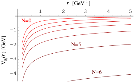
(a)

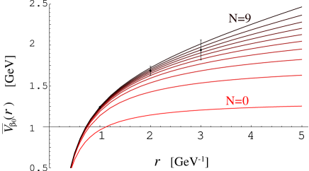
(b)

Figure 1: The QCD potential in the large-$\beta_{0}$ approximation truncated at $O(\alpha_{S}^{N+1})$ term. We set $\mu=2.49$ GeV, $n_{l}=4$ and $\alpha_{S}(\mu)=0.273$ [corresponding to $\alpha_{S}^{(5)}(M_{Z})=0.1181$]. (a) Before subtraction of the leading renormalon. (b) After subtraction of the leading renormalon.

In Fig. 1(a) we show the QCD potential in the large-$\beta_{0}$ approximation truncated at the $(N\!+\!1)$-th term, $\sum_{n=0}^{N}V^{(n)}_{\beta_{0}}(r)$, for $N=0,1,2,\dots$ and $n_{l}=4$. We see that the higher order corrections are indeed large and almost constant (independent of $r$).

It was found [17, 18] that the leading renormalon contained in the QCD potential gets cancelled in the total energy of a static quark-antiquark pair,

$$E_{\rm tot}(r)\equiv 2m_{\rm pole}+V_{\rm QCD}(r),$$ (7)

if the pole mass $m_{\rm pole}$ is expressed in terms of the $\overline{\rm MS}$ mass. Namely, when expressed in terms of the $\overline{\rm MS}$ mass and in a series expansion in $\alpha_{S}(\mu)$, the pole mass contains the leading renormalon [23] which is one half in size and opposite in sign of the leading renormalon of $V_{\rm QCD}(r)$. Thus, the total energy $E_{\rm tot}(r)$ is free from the leading renormalon uncertainties. $E_{\rm tot}(r)$ possesses a residual uncertainty originating from the next-to-leading renormalon [2],

$$\delta E_{\rm tot}(r)\sim\Lambda\times(\Lambda r)^{2},$$ (8)

which is smaller than the leading renormalon uncertainty in the range $r\hbox{ \raise 3.0pt\hbox to0.0pt{$<$}\raise-3.0pt\hbox{$\sim$} }\Lambda^{-1}$. Shown in Fig. 1(b) is the QCD potential in the large-$\beta_{0}$ approximation [truncated at the $(N\!+\!1)$-th term] after the leading renormalon is subtracted at each order of $\alpha_{S}(\mu)$:

$$\overline{V}_{\beta_{0}}(r)=\sum_{n=0}^{\infty}\left[V^{(n)}_{\beta_{0}}(r)+C_{F}\,4\pi\alpha_{S}(\mu)\cdot\frac{\mu\,e^{5/6}}{2\pi^{2}}\cdot\biggl{\{}\frac{\beta_{0}\alpha_{S}(\mu)}{2\pi}\biggr{\}}^{n}\,\,n!\,\right].$$ (9)

One sees that the series expansion of the potential has become much more convergent as compared to Fig. 1(a). For a particular choice of the scale $\mu=2.49$ GeV, the term on the right-hand-side of Eq. (9) becomes smallest at around $n=7$ in the range $1~{}{\rm GeV}^{-1}<r<5~{}{\rm GeV}^{-1}$. Hence, the error bars corresponding to the next-to-leading renormalon uncertainty $\pm{\frac{1}{2}}\Lambda\cdot(\Lambda r)^{2}$ (taking $\Lambda=300$ MeV) are attached to the potential for $N=7$ in the same figure. We may consider that the line for $N=7$ together with the error bars indicate a typical accuracy of the perturbative prediction for the QCD potential, when the leading renormalon is cancelled. We see that the potential is bent upwards at long distances as compared to the leading Coulomb potential ($N=0$). If we choose a smaller scale for $\mu$, the term becomes smallest at a smaller $n$. In this case, convergence properties become better at larger $r$, where we obtain a value of $\overline{V}_{\beta_{0}}(r)$ consistent with $N=7$ of Fig. 1(b) with less terms (smaller $N$). Similarly to the leading renormalon case, the uncertainty is $\mu$-independent, nonetheless.

3 The Total Energy of a $q\bar{q}$ System

Now we examine the total energy of a quark-antiquark pair, defined in Eq. (7), exactly up to ${\cal O}(\alpha_{S}^{3})$. This quantity is free from the leading renormalon uncertainty; in fact the cancellation of the leading renormalons occurs at a deeper level than what can be seen in the large-$\beta_{0}$ approximation [18]. We also note that the cancellation at each order of perturbative expansion is realized only when we use the same coupling constant in expanding $m_{\rm pole}$ and $V_{\rm QCD}(r)$.

The QCD potential of the theory with $n_{l}$ massless flavors only is given, up to ${\cal O}(\alpha_{S}^{3})$, by

$$V_{\rm QCD}(r) = -\,C_{F}\frac{\alpha_{S}(\mu)}{r}\Biggl{[}\,1+\biggl{(}\frac{\alpha_{S}(\mu)}{4\pi}\biggr{)}(2\beta_{0}\ell+a_{1})$$ (10)

$$~{}~{}~{}~{}~{}~{}~{}~{}~{}~{}~{}~{}~{}~{}+\biggl{(}\frac{\alpha_{S}(\mu)}{4\pi}\biggr{)}^{2}\left\{\beta_{0}^{2}\Bigl{(}4\ell^{2}+\frac{\pi^{2}}{3}\Bigr{)}+2(\beta_{1}+2\beta_{0}a_{1})\ell+a_{2}\right\}\Biggr{]},$$

where [24]

$$\ell=\log(\mu r)+\gamma_{E},$$ (11)

$$\beta_{0}=11-\frac{2}{3}n_{l},~{}~{}~{}~{}~{}~{}\beta_{1}=102-\frac{38}{3}n_{l},$$ (12)

$$a_{1}=\frac{31}{3}-\frac{10}{9}n_{l},~{}~{}~{}~{}~{}a_{2}={\frac{4343}{18}}+36\,{{\pi}^{2}}+66\,{\zeta_{3}}-{\frac{9\,{{\pi}^{4}}}{4}}-{n_{l}}\,\left({\frac{1229}{27}}+{\frac{52\,{\zeta_{3}}}{3}}\right)+{\frac{100}{81}}\,{n_{l}^{2}}.$$

The relation between the pole mass and the $\overline{\rm MS}$ mass has been computed up to three loops in a full theory, which contains $n_{h}$ heavy flavors and $n_{l}$ massless flavors [25]. (The same relation was obtained numerically in [26] in a certain approximation.) Rewriting the relation in terms of the coupling of the theory with $n_{l}$ massless flavors only, we find

$$m_{{\rm pole}}=\overline{m}\left\{1+{4\over 3}\,{\alpha_{S}(\overline{m})\over\pi}+\left({\alpha_{S}(\overline{m})\over\pi}\right)^{2}d_{1}+\left({\alpha_{S}(\overline{m})\over\pi}\right)^{3}d_{2}\right\},$$ (14)

where $\overline{m}\equiv m_{\overline{\rm MS}}(m_{\overline{\rm MS}})$ denotes the renormalization-group-invariant $\overline{\rm MS}$ mass, and

$$d_{1} = {\frac{3049}{288}}+{\frac{2\,{{\pi}^{2}}}{9}}+{\frac{{{\pi}^{2}}\,\log 2}{9}}-{\frac{{\zeta_{3}}}{6}}+{n_{l}}\,\left(-{\frac{71}{144}}-{\frac{{{\pi}^{2}}}{18}}\right)+{n_{h}}\,\left(-{\frac{143}{144}}+{\frac{{{\pi}^{2}}}{9}}\right),$$ (15)

$$d_{2} = {\frac{1145453}{10368}}+{\frac{25379\,{{\pi}^{2}}}{2592}}+{\frac{235\,{{\pi}^{2}}\,\log 2}{54}}-{\frac{9\,\zeta_{3}}{8}}-{\frac{341\,{{\pi}^{4}}}{2592}}-{\frac{7\,{{\pi}^{2}}\,{\log^{2}2}}{27}}$$ (16)

$$-{\frac{19\,{\log^{4}2}}{54}}-{\frac{76\,a_{4}}{9}}-{\frac{1331\,{{\pi}^{2}}\,\zeta_{3}}{432}}+{\frac{1705\,\zeta_{5}}{216}}$$

$$+n_{l}\Biggl{(}-{\frac{81227}{7776}}-{\frac{965\,{{\pi}^{2}}}{648}}-{\frac{11\,{{\pi}^{2}}\,\log 2}{81}}-{\frac{707\,\zeta_{3}}{216}+{\frac{61\,{{\pi}^{4}}}{1944}}+{\frac{2\,{{\pi}^{2}}\,{\log^{2}2}}{81}}+{\frac{{\log^{4}2}}{81}}+{\frac{8\,a_{4}}{27}}}\Biggr{)}$$

$$+n_{h}\Biggl{(}-{\frac{157007}{7776}}+{\frac{13627\,{{\pi}^{2}}}{1944}}-{\frac{640\,{{\pi}^{2}}\,\log 2}{81}}+{\frac{751\,\zeta_{3}}{216}}+{\frac{41\,{{\pi}^{4}}}{972}}-{\frac{{{\pi}^{2}}\,{\log^{2}2}}{81}}+{\frac{{\log^{4}2}}{81}}$$

$$~{}~{}~{}~{}~{}~{}~{}~{}+{\frac{8\,a_{4}}{27}}-{\frac{{{\pi}^{2}}\,\zeta_{3}}{4}}+{\frac{5\,\zeta_{5}}{4}}\Biggr{)}$$

$$+n_{l}^{2}\Biggl{(}{\frac{2353}{23328}}+{\frac{13\,{{\pi}^{2}}}{324}}+{\frac{7\,\zeta_{3}}{54}}\Biggr{)}+n_{l}\,n_{h}\Biggl{(}{\frac{5917}{11664}}-{\frac{13\,{{\pi}^{2}}}{324}}-{\frac{2\,\zeta_{3}}{27}}\Biggr{)}$$

$$+n_{h}^{2}\Biggl{(}{\frac{9481}{23328}}-{\frac{4\,{{\pi}^{2}}}{405}}-{\frac{11\,\zeta_{3}}{54}}\Biggr{)},$$

with $a_{4}={\rm Li}_{4}(\frac{1}{2})$. Furthermore, we rewrite $\alpha_{S}(\overline{m})$ in terms of $\alpha_{S}(\mu)$ using the renormalization-group evolution of the coupling constant. Thus, we examine the series expansion of $E_{\rm tot}(r;\overline{m},\alpha_{S}(\mu))$ in $\alpha_{S}(\mu)$ up to ${\cal O}(\alpha_{S}^{3})$. Qualitatively the series shows a convergence property very similar to $\overline{V}_{\beta_{0}}(r)$ for $N=0,1,2$; cf. Fig. 1(b).

The obtained total energy depends on the scale $\mu$ due to truncation of the series at a finite order. One finds that, when $r$ is small, the series converges better and the value of $E_{\rm tot}(r)$ is less $\mu$-dependent if we choose a large scale for $\mu$, whereas when $r$ is larger, the series converges better and the value of $E_{\rm tot}(r)$ is less $\mu$-dependent if we choose a smaller scale for $\mu$. Taking into account this property, we will fix the scale $\mu$ in two different ways below:

1. We fix the scale $\mu=\mu_{1}(r)$ by demanding stability against variation of the scale:

   $$\left.\mu\frac{d}{d\mu}E_{\rm tot}(r;\overline{m},\alpha_{S}(\mu))\right|_{\mu=\mu_{1}(r)}=0.$$ (17)

2. We fix the scale $\mu=\mu_{2}(r)$ on the minimum of the absolute value of the last known term [${\cal O}(\alpha_{S}^{3})$ term] of $E_{\rm tot}(r)$:

   $$\left.\mu\frac{d}{d\mu}\Bigl{[}E^{(3)}_{\rm tot}(r;\overline{m},\alpha_{S}(\mu))\Bigr{]}^{2}\,\right|_{\mu=\mu_{2}(r)}=0.$$ (18)

In this analysis we examine the total energy of a $b\bar{b}$ system. We set $\overline{m}_{b}\equiv m_{b}^{\overline{\rm MS}}(m_{b}^{\overline{\rm MS}})=4.203$ GeV, which is taken from [12]. (Its error is estimated to be about $\pm 30$ MeV.) For simplicity we analyze $E_{\rm tot}(r)$ in two hypothetical cases: (i) when $m_{c}=0$ ($n_{l}=4$ and $n_{h}=1$), and (ii) in the limit $m_{c}\to m_{b}$ ($n_{l}=3$ and $n_{h}=2$). The real world lies somewhere in between the two cases: the charm quark decouples in the excited states of bottomonium but not in the ground state [27]. A more precise analysis requires inclusion of nonzero $m_{c}$ effects into $E_{\rm tot}(r)$, which will be reported elsewhere [28]. The input value of the strong coupling constant is $\alpha_{S}^{(5)}(M_{Z})=0.1181$ [29]. We evolve the coupling and match it to the couplings of the theory with $n_{l}=4$ and 3 successively by solving the renormalization-group equation numerically with the 3-loop beta function and by using the 3-loop matching condition [31] (3-loop running).

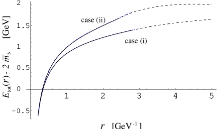
(a)

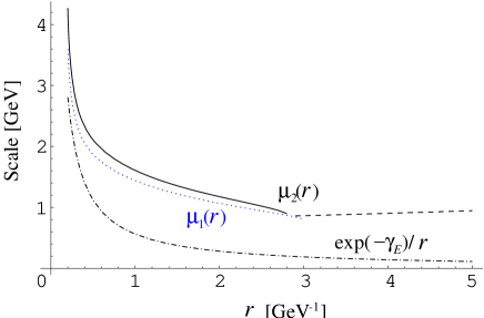
(b)

Figure 2: (a) The total energy of a $b\bar{b}$ system measured from $2\overline{m}_{b}$ in two hypothetical cases. In each case, the scale is fixed by $\mu=\mu_{1}(r)$ (dotted lines) or $\mu=\mu_{2}(r)$ (solid lines if $E_{\rm tot}^{(3)}(r)=0$; dashed lines if $|E_{\rm tot}^{(3)}(r)|>0$). (b) The scales chosen by the scale-fixing prescriptions (17) and (18) in case (i). The notations are same as in (a). A conventional scale choice $\mu=\exp(-\gamma_{E})/r$ is also shown (dotdashed line).

Fig. 2(a) shows $E_{\rm tot}(r)$ (measured from $2\overline{m}_{b}$) for the two cases (i) and (ii). In each case $E_{\rm tot}(r)$ are plotted with the two different scale-fixing prescriptions; the total energy hardly changes whether we choose $\mu=\mu_{1}(r)$ or $\mu=\mu_{2}(r)$. In case (i), the minimal sensitivity scale $\mu_{1}(r)$ exists only in the range $r\hbox{ \raise 3.0pt\hbox to0.0pt{$<$}\raise-3.0pt\hbox{$\sim$} }3$ GeV^-1; for the choice $\mu=\mu_{2}(r)$, the minimum value of $|E^{(3)}_{\rm tot}(r)|$ is zero in the range $r\hbox{ \raise 3.0pt\hbox to0.0pt{$<$}\raise-3.0pt\hbox{$\sim$} }3$ GeV^-1, whereas $|E^{(3)}_{\rm tot}(r)|>0$ in the range $r\hbox{ \raise 3.0pt\hbox to0.0pt{$>$}\raise-3.0pt\hbox{$\sim$} }3$ GeV^-1. These features indicate an instability of the perturbative prediction for $E_{\rm tot}(r)$ at $r\hbox{ \raise 3.0pt\hbox to0.0pt{$>$}\raise-3.0pt\hbox{$\sim$} }3$ GeV^-1. The scales $\mu_{1}(r)$ and $\mu_{2}(r)$ are shown as functions of $r$ in Fig. 2(b). For comparison, we also show $\mu=\exp(-\gamma_{E})/r$, which has been considered as a natural scale of the QCD potential, $V_{\rm QCD}(r)$, conventionally. One sees that $\mu_{1}(r)$ and $\mu_{2}(r)$ are considerably larger than $\exp(-\gamma_{E})/r$. The scales chosen in case (ii) are similar.

	case (i)
	$\mu=\mu_{1}(r)$			$\mu=\mu_{2}(r)$
	$E_{\rm tot}^{(1)}(r)$	$E_{\rm tot}^{(2)}(r)$	$E_{\rm tot}^{(3)}(r)$	$E_{\rm tot}^{(1)}(r)$	$E_{\rm tot}^{(2)}(r)$	$E_{\rm tot}^{(3)}(r)$
$r=1~{}{\rm GeV}^{-1}$	797	69	$-17$	750	98	0
$r=2~{}{\rm GeV}^{-1}$	1255	$-14$	$-17$	1173	48	0
$r=3~{}{\rm GeV}^{-1}$	1709	$-290$	$13$	1606	$-185$	9
	case (ii)
	$\mu=\mu_{1}(r)$			$\mu=\mu_{2}(r)$
	$E_{\rm tot}^{(1)}(r)$	$E_{\rm tot}^{(2)}(r)$	$E_{\rm tot}^{(3)}(r)$	$E_{\rm tot}^{(1)}(r)$	$E_{\rm tot}^{(2)}(r)$	$E_{\rm tot}^{(3)}(r)$
$r=1~{}{\rm GeV}^{-1}$	962	70	$-32$	879	117	0
$r=2~{}{\rm GeV}^{-1}$	1659	$-116$	$-31$	1502	4	0
$r=3~{}{\rm GeV}^{-1}$	–	–	–	1994	$-197$	70

Table 1: Series expansion of the total energy in $\alpha_{S}(\mu)$ with the two scale choices Eqs. (17) and (18). $E_{\rm tot}^{(n)}(r)$ denotes the ${\cal O}(\alpha_{S}^{n})$ term of $E_{\rm tot}(r)$. All numbers are in MeV unit. The minimal sensitivity scale $\mu_{1}(r)$ exists only at $r<2.8~{}{\rm GeV}^{-1}$ in case (ii).

In Table 1 we show each term of the series expansion of $E_{\rm tot}(r)$. The series shows healthy convergent behavior at $r\hbox{ \raise 3.0pt\hbox to0.0pt{$<$}\raise-3.0pt\hbox{$\sim$} }3~{}{\rm GeV}^{-1}$.

At this stage, let us discuss why the scales $\mu_{1}(r)$ and $\mu_{2}(r)$ are considerably larger than $\exp(-\gamma_{E})/r$. For this purpose we use an approximate expression for the pole mass, which follows from the fact that the dominant contribution to the pole-$\overline{\rm MS}$ mass relation can be read from the infrared region, loop momenta $q\ll\overline{m}$, of the QCD static potential [18]:

$$2m_{\rm pole}\approx 2\overline{m}+{\hbox to18.0pt{ \hbox to-5.0pt{$\displaystyle\int$} \raise-19.0pt\hbox{$\scriptstyle|\vec{q}|<\overline{m}$} }}\frac{d^{3}\vec{q}}{(2\pi)^{3}}\,|V_{\rm QCD}(q)|=2\overline{m}+\frac{2C_{F}}{\pi}\int_{0}^{\overline{m}}dq\,\tilde{\alpha}_{V}(q).$$ (19)

Here, $V_{\rm QCD}(q)=-C_{F}4\pi\tilde{\alpha}_{V}(q)/q^{2}$ is the QCD static potential in momentum space. Then the total energy can be written approximately as

$$E_{\rm tot}(r) \approx 2\overline{m}+\int\frac{d^{3}\vec{q}}{(2\pi)^{3}}\,|V_{\rm QCD}(q)|\,\Bigl{[}\,\theta(\overline{m}-q)-\exp(i\vec{q}\cdot\vec{r})\,\Bigr{]}$$ (20)

$$= 2\overline{m}+\frac{2C_{F}}{\pi}\int_{0}^{\infty}dq\,\tilde{\alpha}_{V}(q)\,\left[\theta(\overline{m}-q)-\frac{\sin(qr)}{qr}\right].$$ (21)

In the integrands, the factors in the brackets $[\cdots]$ are appreciable only in the range $1/r\hbox{ \raise 3.0pt\hbox to0.0pt{$<$}\raise-3.0pt\hbox{$\sim$} }q<\overline{m}$. So, roughly speaking, $E_{\rm tot}(r)$ is determined from an average $\left<\tilde{\alpha}_{V}\right>$ of the $V$-scheme coupling $\tilde{\alpha}_{V}(q)$ over the range $1/r\hbox{ \raise 3.0pt\hbox to0.0pt{$<$}\raise-3.0pt\hbox{$\sim$} }q<\overline{m}$. When evaluating this quantity in fixed-order perturbation theory, a scale $\mu(r)$ which represents this average coupling, i.e. $\tilde{\alpha}_{V}(\mu(r))\approx\left<\tilde{\alpha}_{V}\right>$, would be a most natural scale. Such a scale should lie between $1/r$ and $\overline{m}$. This argument is in contrast with the conventional principle for the scale choice for the QCD potential $V_{\rm QCD}(r)$. Apart from $\Lambda_{\rm QCD}$, the QCD potential contains only one scale $1/r$, so that the choice of scale has been almost automatic, $\mu\sim 1/r$. The potential alone, however, has a large uncertainty due to the leading renormalon. It stems from the contribution of $\tilde{\alpha}_{V}(q)$ at $q\sim\Lambda_{\rm QCD}$. On the other hand, the total energy is free from the leading renormalons by cutting out large contributions from $\Lambda_{\rm QCD}\sim q<1/r$ as seen in Eq. (21). Consequently the relevant scale is shifted to higher momentum region in comparison to that of $V_{\rm QCD}(r)$.

It would also be instructive to compare the above scale choices with the Brodsky-Lepage-Mackenzie (BLM) scale-fixing prescription [30] applied to $V_{\rm QCD}(r)$ and $E_{\rm tot}(r)$, respectively. In this prescription (at the lowest order), the part of higher-order corrections to $V_{\rm QCD}(r)$ or to $E_{\rm tot}(r)$ given by the large-$\beta_{0}$ approximation is absorbed into the scale choice. For the QCD potential, at the lowest order the BLM scale is fixed as $\mu=\exp(-\frac{5}{6}-\gamma_{E})/r\approx 0.43\,\exp(-\gamma_{E})/r$. For the total energy, the BLM scale at the lowest order is given by $\mu=f(\overline{m}r)/r$, where

$$f(x)=\exp\left[\Bigl{(}\log x-\frac{\pi^{2}}{8}+\gamma_{E}-\frac{53}{192}\Bigr{)}\frac{x}{x-\frac{\pi}{2}}-\frac{5}{6}-\gamma_{E}\right].$$ (22)

Due to the singularity of $f(x)$ at $x=\pi/2$, the BLM scale turns out to be unstable around $r=\pi/(2\overline{m})$. This is because the coefficient of $\beta_{0}\log\mu$ in $E_{\rm tot}(r;\overline{m},\alpha_{S}(\mu))$ becomes small by a cancellation between $V_{\rm QCD}(r)$ and $2m_{\rm pole}$. In this region of $r$, the BLM prescription for $E_{\rm tot}(r)$ would be unreliable. For $r>\pi/(2\overline{m})$, the function $f(\overline{m}r)$ increases monotonically. Setting $\overline{m}=4.203$ GeV, we find that at $r\hbox{ \raise 3.0pt\hbox to0.0pt{$>$}\raise-3.0pt\hbox{$\sim$} }0.6~{}{\rm GeV}^{-1}$ the scale $\mu=f(\overline{m}r)/r$ exceeds the BLM scale of the QCD potential; at $r\hbox{ \raise 3.0pt\hbox to0.0pt{$>$}\raise-3.0pt\hbox{$\sim$} }1~{}{\rm GeV}^{-1}$, $\mu=f(\overline{m}r)/r$ becomes almost independent of $r$, $\mu\approx 0.5$ GeV, converging towards the BLM scale of the pole mass. These features in the region $r\hbox{ \raise 3.0pt\hbox to0.0pt{$>$}\raise-3.0pt\hbox{$\sim$} }0.6~{}{\rm GeV}^{-1}$ are consistent with the results of the analysis given in Sec. 2. Since the higher-order corrections are large for $V_{\beta_{0}}(r)$, the BLM scale of $V_{\rm QCD}(r)$ tends to be small. On the other hand, since the higher-order corrections are smaller for $\overline{V}_{\beta_{0}}(r)$, the BLM scale of $E_{\rm tot}(r)$ is larger. Intuitively the BLM scale of a quantity sensitive to renormalons is attracted towards the $\Lambda_{\rm QCD}$ scale, whereas that of a renormalon-free quantity is determined by a short-distance scale. Thus, the qualitative features of the BLM scales agree with those of the scales shown in Fig. 2(b) in the range $1~{}{\rm GeV}^{-1}\hbox{ \raise 3.0pt\hbox to0.0pt{$<$}\raise-3.0pt\hbox{$\sim$} }r\hbox{ \raise 3.0pt\hbox to0.0pt{$<$}\raise-3.0pt\hbox{$\sim$} }5~{}{\rm GeV}^{-1}$, although the level of agreement is not very accurate. At shorter distances $r\approx\pi/(2\overline{m})$, validity of the BLM prescription for the total energy seems doubtful on account of the large cancellation.

We return to the discussion of $E_{\rm tot}(r)$.

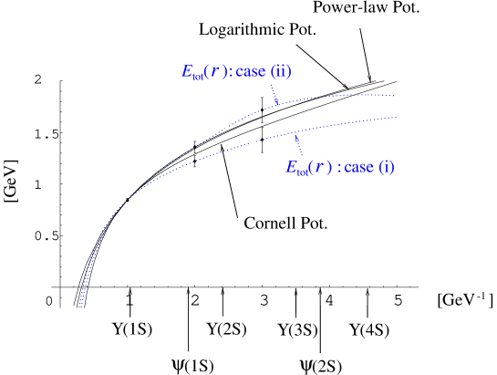
Figure 3: A comparison of the total energy of a $b\bar{b}$ system in the two hypothetical cases (dotted lines) and typical phenomenological potentials (solid lines). For a reference, we show typical sizes of the bottomonium and charmonium $S$ states as determined from the r.m.s. interquark distances with respect to the Cornell potential: $\sqrt{\left<r^{2}\right>}_{\rm Cornell}$.

In Fig. 3 we compare the total energies in case (i) and (ii) with typical phenomenological potentials used in phenomenological approaches. We take:

• A Coulomb-plus-linear potential (Cornell potential) [32]:

  $$V(r)=-\frac{\kappa}{r}+\frac{r}{a^{2}}$$ (23)

  with $\kappa=0.52$ and $a=2.34$ GeV^-1.

• A power-law potential [33]:

  $$V(r)=-8.064~{}{\rm GeV}+(6.898~{}{\rm GeV})(r\times 1~{}{\rm GeV})^{0.1}.$$ (24)

• A logarithmic potential [34]:

  $$V(r)=-0.6635~{}{\rm GeV}+(0.733~{}{\rm GeV})\log(r\times 1~{}{\rm GeV}).$$ (25)

We may consider the differences of these potentials in the range $0.5~{}{\rm GeV}^{-1}\hbox{ \raise 3.0pt\hbox to0.0pt{$<$}\raise-3.0pt\hbox{$\sim$} }r\hbox{ \raise 3.0pt\hbox to0.0pt{$<$}\raise-3.0pt\hbox{$\sim$} }5~{}{\rm GeV}^{-1}$ as uncertainties of the phenomenologically determined potentials. In order to make a clear comparison, arbitrary constants have been added to all the potentials and $E_{\rm tot}(r)$ such that their values coincide at $r=1$ GeV^-1. As stated, we expect the perturbative prediction for a realistic $E_{\rm tot}(r)$ to lie between those for the cases (i) and (ii). It appears to be in good agreement with the phenomenological potentials in the above range. The level of agreement is consistent with the uncertainties expected from the next-to-leading renormalon contributions (indicated by the error bars).

4 The Interquark Force

Instead of the total energy, we may also consider the interquark force defined by

$$F(r) \equiv -\frac{d}{dr}E_{\rm tot}(r)=-\frac{d}{dr}V_{\rm QCD}(r)$$ (26)

$$\equiv -C_{F}\frac{\alpha_{F}(1/r)}{r^{2}}.$$ (27)

The last line defines the “$F$-scheme” coupling constant $\alpha_{F}(\mu)$. The interquark force is also free from the leading renormalon. In fact it has been noted [35] that the perturbative expansion of $F(r)$ is more convergent than that of the potential $V_{\rm QCD}(r)$. Since in the zero quark mass limit $F(r)$ is dependent only on $r$, we may determine its $r$-dependence using the renormalization-group equation:

$$\mu^{2}\frac{d}{d\mu^{2}}\alpha_{F}(\mu)=\beta_{F}(\alpha_{F}).$$ (28)

It is instructive to compare the beta functions for the couplings defined in the three different schemes. For $n_{l}=4$, we find

$$\begin{array}[]{lcclclclclcl}\beta_{V}(\alpha_{V})&=&-&0.6631\,{\alpha_{V}^{2}}&-&0.3251\,{\alpha_{V}^{3}}&-&1.7527\,{\alpha_{V}^{4}}&+&{\cal O}(\alpha_{V}^{5})&{}{}{}{}\hfil&\mbox{($V$-scheme)}\\ \beta_{F}(\alpha_{F})&=&-&0.6631\,{\alpha_{F}^{2}}&-&0.3251\,{\alpha_{F}^{3}}&-&0.5861\,{\alpha_{F}^{4}}&+&{\cal O}(\alpha_{F}^{5})&{}{}{}{}\hfil&\mbox{($F$-scheme)}\\ \beta_{\overline{\rm MS}}(\alpha_{S})&=&-&0.6631\,{\alpha_{S}^{2}}&-&0.3251\,{\alpha_{S}^{3}}&-&0.2048\,{\alpha_{S}^{4}}&+&{\cal O}(\alpha_{S}^{5})&{}{}{}{}\hfil&\mbox{($\overline{\rm MS}$-scheme)}\end{array}$$ (32)

The first two coefficients of the beta functions are scheme-independent (when we neglect the quark masses). The third coefficient of the $V$-scheme beta function is quite large, reflecting poor convergence of $V_{\rm QCD}(r)$ due to the leading renormalons. The third coefficient of the $F$-scheme beta function is smaller by factor 3 due to cancellation of the leading renormalon. The third coefficient of the $\overline{\rm MS}$-scheme beta function is even smaller by factor 3. This may be due to the fact that the $F$-scheme coupling still contains the next-to-leading renormalon contributions. From this comparison, we may conclude that it is better to analyze $F(r)$ rather than $V_{\rm QCD}(r)$ as a physical quantity, in perturbative analyses.

The observed bottomonium spectrum is qualitatively very different from the Coulomb spectrum. The largest difference is that, the level spacings between consecutive bottomonium $nS$ states are almost constant, whereas in the Coulomb spectrum the level spacings decrease as $1/n^{2}$. When we consider effects of the QCD radiative corrections on the lowest-order Coulomb potential, one may interpret that in the QCD potential, $-C_{F}\alpha_{V}(1/r)/r$, the $V$-scheme coupling increases at long distances, so that the potential will be bent downwards. This is obviously a bad interpretation, because in such a case, the level spacings among the excited states become even smaller than those of the Coulomb spectrum. We should rather consider the interquark force. A better interpretation is that in $F(r)=-C_{F}\alpha_{F}(1/r)/r^{2}$, the $F$-scheme coupling increases at long distances, and $|F(r)|$ grows correspondingly. This means that the slope of the potential becomes steeper at long distances. (Its effect resembles an addition of a linearly rising potential to the Coulomb potential.) Accordingly the level spacings among the excited states increase. Thus, the effects of the radiative corrections on the level spacings are even qualitatively reversed, whether we consider $V_{\rm QCD}(r)$ or $F(r)$ as the physically relevant quantity.

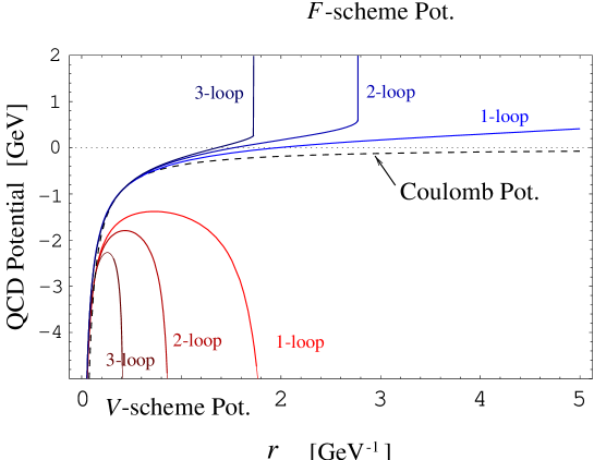
Figure 4: A comparison of the QCD potentials calculated in $V$-scheme and in $F$-scheme as well as the Coulomb potential. The Coulomb potential is given by $-C_{F}\alpha/r$ with $\alpha=0.279$. The $V$-scheme and $F$-scheme potentials correspond to $\alpha_{S}^{(5)}(M_{Z})=0.1181$.

One may verify these features in Fig. 4, in which the Coulomb potential, the $V$-scheme potentials and the $F$-scheme potentials are displayed. The $V$-scheme potentials are calculated by solving the renormalization-group equation for $\alpha_{V}$ numerically, using $\beta_{V}$ in Eq. (32) up to order $\alpha_{V}^{2}$ (1-loop), order $\alpha_{V}^{3}$ (2-loop) and order $\alpha_{V}^{4}$ (3-loop). The $F$-scheme potentials are calculated by first solving the renormalization-group equation for $\alpha_{F}$ numerically via $\beta_{F}$ in Eq. (32) and then by integrating $-F(r)$ over $r$ numerically; arbitrary constants are added such that the $F$-scheme potentials coincide the Coulomb potential at $r=0.4$ GeV^-1. The initial values for $\alpha_{V}$ and $\alpha_{F}$ are given at $r=\exp(-\gamma_{E})/\overline{m}_{b}$ by matching to the fixed-order results. As can be seen, the $V$-scheme potentials become singular at fairly short distances, $r\sim 2$ GeV^-1 (1-loop), 0.9 GeV^-1 (2-loop), and 0.4 GeV^-1 (3-loop), respectively. As expected, the $F$-scheme potentials have wider ranges of validity: they become singular at $r\sim 6.9$ GeV^-1 (1-loop), 2.8 GeV^-1 (2-loop), and 1.7 GeV^-1 (3-loop), respectively. The situation is puzzling, however, in that the predictable range reduces as we include more terms of $\beta_{F}(\alpha_{F})$. The 2-loop and 3-loop $F$-scheme potentials are consistent with the phenomenological potentials within the uncertainty expected from the next-to-leading renormalon contributions, in the range $0.5~{}{\rm GeV}^{-1}\hbox{ \raise 3.0pt\hbox to0.0pt{$<$}\raise-3.0pt\hbox{$\sim$} }r\hbox{ \raise 3.0pt\hbox to0.0pt{$<$}\raise-3.0pt\hbox{$\sim$} }2.8~{}{\rm GeV}^{-1}$ and $0.5~{}{\rm GeV}^{-1}\hbox{ \raise 3.0pt\hbox to0.0pt{$<$}\raise-3.0pt\hbox{$\sim$} }r\hbox{ \raise 3.0pt\hbox to0.0pt{$<$}\raise-3.0pt\hbox{$\sim$} }1.7~{}{\rm GeV}^{-1}$, respectively. On the other hand, the 1-loop $F$-scheme potential does not satisfy this criterion.

If we take a larger input value for $\alpha_{S}^{(5)}(M_{Z})$, the slopes of the $F$-scheme potentials get steeper, since $\alpha_{F}$ increases. Also, it explains why $E_{\rm tot}(r)$ for case (ii) is steeper than that for case (i) in Fig. 2(a): $\alpha_{F}$ for $n_{l}=3$ is larger than that for $n_{l}=4$ at $r\hbox{ \raise 3.0pt\hbox to0.0pt{$>$}\raise-3.0pt\hbox{$\sim$} }1/\overline{m}_{b}$.

5 Conclusions

When we incorporate the cancellation of the leading renormalon contributions, the perturbative expansion of the total energy $E_{\rm tot}(r)$ of a $b\bar{b}$ system, up to ${\cal O}(\alpha_{S}^{3})$ and supplemented by the scale-fixing prescription (17) or (18), converges well at $r\hbox{ \raise 3.0pt\hbox to0.0pt{$<$}\raise-3.0pt\hbox{$\sim$} }3~{}{\rm GeV}^{-1}$. Moreover, it agrees with the phenomenologically determined potentials in the range $0.5~{}{\rm GeV}^{-1}\hbox{ \raise 3.0pt\hbox to0.0pt{$<$}\raise-3.0pt\hbox{$\sim$} }r\hbox{ \raise 3.0pt\hbox to0.0pt{$<$}\raise-3.0pt\hbox{$\sim$} }3~{}{\rm GeV}^{-1}$ within the uncertainty expected from the next-to-leading renormalon contributions. Even at $r\hbox{ \raise 3.0pt\hbox to0.0pt{$>$}\raise-3.0pt\hbox{$\sim$} }3~{}{\rm GeV}^{-1}$, the scale-fixing prescription (18) gives a reasonable prediction for $E_{\rm tot}(r)$; it appears that the perturbative prediction does not break down suddenly but rather the uncertainty grows gradually as $r$ increases. The agreement is unlikely to be accidental, since as soon as we take the input $\alpha_{S}^{(5)}(M_{Z})$ outside of the present world average values $0.1181\pm 0.0020$ [29], the agreement is lost quickly.

A non-relativistic Hamiltonian

$$H=2m_{\rm pole}+\vec{p}\,^{2}/m_{\rm pole}+V_{\rm QCD}(r)=\vec{p}\,^{2}/m_{\rm pole}+E_{\rm tot}(r)$$ (33)

constitutes a part of the full Hamiltonian (up to the order $1/c^{2}$) analyzed in [12]. It detetermines the bulk of the quarkonium level structure computed therein. At the same time, the above Hamiltonian is exactly the ones analyzed in the conventional phenomenological potential-model approaches (at the leading order) if $E_{\rm tot}(r)$ is identified with the phenomenological potentials. Also, it is the leading-order Hamiltonian of the more systematic frameworks discussed in Sec. 1. Thus, we find that the agreement of $E_{\rm tot}(r)$ and the phenomenologically determined potentials is the reason why the gross structure of the bottomonium spectrum is reproduced well by the computation based on perturbative QCD. Our observation confirms the conclusion of [12], that once the leading renormalon contributions are cancelled, there remain no large non-perturbative effects, which essentially deteriorate perturbative treatment of some of the bottomonium and charmoninum states, but only moderate contributions comparable in size with the next-to-leading renormalons.

Similarly, if we analyze the interquark force $F(r)$ instead of $V_{\rm QCD}(r)$, the range of perturbative predictability becomes significantly wider, as known from the previous study [35]. We confirm this observation using a renormalization-group analysis. We find that the 2-loop and 3-loop renormalization-group-improved potentials, obtained by integrating $-F(r)$, are consistent with the phenomenological potentials up to $r\sim 2.8~{}{\rm GeV}^{-1}$ and $r\sim 1.7~{}{\rm GeV}^{-1}$, respectively.

We expect that the connection elucidated in this work will be useful for developing deeper theoretical understandings of the bottomonium and charmonium systems. For more detailed comparisons, in general it would be more secure to compute the quarkonium spectra directly rather than $E_{\rm tot}(r)$ or $F(r)$. Indeed, the series expansions of the quarkonium energy levels turn out to be more convergent when we include the full corrections ($\vec{p}\,^{4}$-term, Darwin potential, spin-dependent potentials, etc.) to the ${\cal O}(1/c^{2})$ Hamiltonian, as compared to the expansions of the energy levels of the simplified Hamiltonian (33) (even after the leading renormalons are cancelled).

References

- [1] E. Eichten and C. Quigg, Phys. Rev. D49, 5845 (1994).
- [2] U. Aglietti and Z. Ligeti, Phys. Lett. B364, 75 (1995).
- [3] L. Brown and W. Weisberger, Phys. Rev. D20, 3239 (1979).
- [4] E. Eichten and F. Feinberg, Phys. Rev. Lett. 43, 1205 (1979); Phys. Rev. D23, 2724 (1981).
- [5] D. Gromes, Z. Phys. C22, 265 (1984).
- [6] A. Barchielli, E. Montaldi and G. Prosperi, Nucl. Phys. B296, 625 (1988), erratum, B303, 752;
- [7] A. Barchielli, N. Brambilla and G. Prosperi, Nuovo Cim. 103A, 59 (1990).
- [8] A. Pineda and J. Soto, Nucl. Phys. Proc. Suppl. 64, 428 (1998).
- [9] N. Brambilla, A. Pineda, J. Soto and A. Vairo, Nucl. Phys. B566, 275 (2000).
- [10] G. Bali, K. Schilling and A. Wachter, Phys. Rev. D56, 2566 (1997).
- [11] UKQCD Collaboration, C. Allton, et al., Phys. Rev. D60, 034507 (1999).
- [12] N. Brambilla, Y. Sumino and A. Vairo, Phys. Lett. B513, 381 (2001).
- [13] S. Titard and F. Yndurain, Phys. Rev. D49, 6007 (1994); Phys. Rev. D51, 6348 (1995).
- [14] A. Pineda and F. Ynduráin, Phys. Rev. D58, 094022 (1998); D61, 077505 (2000).
- [15] K. Melnikov and A. Yelkhovsky, Phys. Rev. D59, 114009 (1999).
- [16] N. Brambilla and A. Vairo, Phys. Rev. D62, 094019 (2000).
- [17] A. Hoang, M. Smith, T. Stelzer and S. Willenbrock, Phys. Rev. D59, 114014 (1999).
- [18] M. Beneke, Phys. Lett. B434, 115 (1998).
- [19] T. Appelquist, M. Dine and I. Muzinich, Phys. Rev. D17, 2074 (1978).
- [20] M. Beneke, hep-ph/9911490.
- [21] Y. Sumino, hep-ph/0004087.
- [22] M. Beneke and V. Braun, Phys. Lett. B348, 513 (1995).
- [23] M. Beneke and V. Braun, Nucl. Phys. B426, 301 (1994); I. Bigi, M. Shifman, N. Uraltsev and A. Vainshtein, Phys. Rev. D50, 2234 (1994).
- [24] M. Peter, Phys. Rev. Lett. 78, 602 (1997); Nucl. Phys. B501 471 (1997); Y. Schröder, Phys. Lett. B447, 321 (1999).
- [25] K. Melnikov and T. v. Ritbergen, Phys. Lett. B482, 99 (2000).
- [26] K. Chetyrkin and M. Steinhauser, Phys. Rev. Lett. 83, 4001 (1999); Nucl. Phys. B573, 617 (2000).
- [27] N. Brambilla, Y. Sumino and A. Vairo, hep-ph/0108084.
- [28] S. Recksiegel and Y. Sumino, hep-ph/0109122.
- [29] D. E. Groom et al., Eur. Phys. Jour. C15, 1 (2000).
- [30] S. Brodsky, G. Lepage and P. Mackenzie, Phys. Rev. D28, 228 (1983).
- [31] S. Larin, T. v. Ritbergen and J. Vermaseren, Nucl. Phys. B438, 278 (1995).
- [32] E. Eichten, K. Gottfried, T. Kinoshita, K. Lane and T. Yan, Phys. Rev. D17, 3090 (1978); D21, 313(E) (1980); D21, 203 (1980).
- [33] A. Martin, Phys. Lett. 93B, 338 (1980).
- [34] C. Quigg and J. Rosner, Phys. Lett. 71B, 153 (1977).
- [35] M. Melles, Phys. Rev. D62, 074019 (2000).
- [36] G. Bali, Phys. Rept. 343, 1 (2001).
- [37] V. Kiselev, A. Kovalsky and A. Onishchenko, Phys. Rev. D64, 054009 (2001).
- [38] G. Grunberg, Phys. Rev. D40, 680 (1989).