Coherence Phenomena
in Charmonium Production off Nuclei
at the Energies of RHIC and LHC

Abstract

In the energy range of RHIC and LHC the mechanisms of nuclear suppression of charmonia are expected to be strikingly different from what is known for the energy of the SPS. One cannot think any more of charmonium produced on a bound nucleon which then attenuates as it passes through the rest of the nucleus. The coherence length of charmonium production substantially exceeds the nuclear radius in the new energy range. Therefore the production amplitudes on different nucleons, rather than the cross sections, add up and interfere, i.e. shadowing is at work. So far no theoretical tool has been available to calculate nuclear effects for charmonium production in this energy regime. We develop a light-cone Green function formalism which incorporates the effects of the coherence of the production amplitudes and of charmonium wave function formation, and is the central result of this paper. We found a substantial deviation from QCD factorization, namely, gluon shadowing is much stronger for charmonium production than it is in DIS. We predict for nuclear effects $x_{2}$ scaling which is violated at lower energies by initial state energy loss which must be also included in order to compare with available data. In this paper only the indirect $J/\Psi$s originating from decay of $P$-wave charmonia are considered. The calculated $x_{F}$-dependence of $J/\Psi$ nuclear suppression is in a good accord with data. We predict a dramatic variation of nuclear suppression with $x_{F}$ in pA and a peculiar peak at $x_{F}=0$ in AA collisions at RHIC.

1 Introduction

Charmonium production off nuclei has drawn much attention during the last two decades since the NA3 experiment at CERN [1] has found a steep increase of nuclear suppression with rising Feynman $x_{F}$. This effect has been confirmed later in the same energy range [2], and at higher energy recently by the most precise experiment E866 at Fermilab [3]. No unambiguous explanation for these observations has been provided yet. With the advent of RHIC new data are expected soon in the unexplored energy range. Lacking a satisfactory understanding of nuclear effects for charmonium production in proton-nucleus collisions it is very difficult to provide a convincing interpretation of data from heavy ion collisions experiments [4, 5] which are aimed to detect the creation of a quark-gluon plasma using charmonium as a sensitive probe. Many of existing analyses rely on an oversimplified dynamics of charmonium production which fails to explain even data for $pA$ collisions, in particular the observed $x_{F}$ dependence of $J/\Psi$ suppression. Moreover, sometimes even predictions for RHIC employ those simple models. It is the purpose of present paper to demonstrate that the dynamics of charmonium suppression strikingly changes between the SPS and RHIC energies. We perform full QCD calculations of nuclear effects within framework of the light-cone Green function approach aiming to explain observed nuclear effects without adjusting any parameters, and to provide realistic predictions for RHIC.

To avoid a confusion, we should make it clear that we will skip discussion of any mechanisms of charmonium suppression caused by the interaction with the produced comoving matter, although it should be an important effect in central heavy ion collisions. Instead, we consider suppression which originates from the production process and propagation of the $\bar{c}c$ pair through the nucleus. It serves as a baseline for search for new physics in heavy ion collisions.

The present paper is focused on coherence phenomena which are still a rather small correction for charmonium production at the SPS, but whose onset is already observed at Fermilab and which are expected to become a dominant effect at the energies of the RHIC and LHC. One realizes the importance of the coherence effects treating charmonium production in an intuitive way as a hard $\bar{c}c$ fluctuation which lose coherence with the projectile ensemble of partons via interaction with the target, and is thus liberated. In spite of the hardness of the fluctuation, its lifetime in the target rest frame increases with energy and eventually exceeds the nucleus size. Apparently, in this case the $\bar{c}c$ pair is freed via interaction with the whole nucleus, rather than with an individual bound nucleon as it happens at low energies. Correspondingly, nuclear effects become stronger at high energies since the fluctuation propagates through the whole nucleus, and different nucleons compete with each other in freeing the $\bar{c}c$. In terms of the conventional Glauber approach it leads to shadowing. In terms of the parton model it is analogous to shadowing of $c$-quarks in the nuclear structure function. It turns out (see Sect. 4) that the fluctuations containing gluons in addition to the $\bar{c}c$ pair are subject to especially strong shadowing. Since at high energies the weight of such fluctuations rises, as well the the fluctuation lifetime, it becomes the main source of nuclear suppression of open and hidden charm at high energies, in particular at RHIC. In terms of the parton model shadowing for such fluctuations containing gluons correspond to gluon shadowing.

The parton model interpretation of charmonium production contains no explicit coherence effects, but they are hidden in the gluon distribution function of the nucleus which is supposed to be subject to QCD factorization. There are, however, a few pitfalls on this way. First of all, factorization is exact only in the limit of a very hard scale. That means that one should neglect the effects of the order of the inverse $c$-quark mass, in particular the transverse $\bar{c}c$ separation $\langle r_{T}^{2}\rangle\sim 1/m_{c}^{2}$. However, shadowing and absorption of $\bar{c}c$ fluctuations is a source of a strong suppression which is nearly factor of $0.5$ for heavy nuclei (see Fig. 4). QCD factorization misses this effect. Second of all, according to factorization gluon shadowing is supposed to be universal, i.e. one can borrow it from another process (although we still have no experimental information about gluons shadowing, it only can be calculated) and use to predict nuclear suppression of open or hidden charm. Again, factorization turns out to be dramatically violated at the scale of charm and gluon shadowing for charmonium production is much stronger than it is for open charm or deep-inelastic scattering (DIS) (compare gluon shadowing exposed in Fig. 7 with one calculated in [6] for DIS). All these important, sometimes dominant effects are missed by QCD factorization. This fact once again emphasizes the advantage of the light-cone dipole approach which does reproduce QCD factorization in situations where that is expected to be at work, and it is also able to calculate the deviations from factorization in a parameter free way.

Unfortunately, none of the existing models for $J/\Psi$ or $\Psi^{\prime}$ production in $NN$ collisions is fully successful in describing all the features observed experimentally. In particular, the $J/\Psi$, $\Psi^{\prime}$ and $\chi_{1}$ production cross sections in $NN$ collisions come out too small by at least an order of magnitude [7]. Only data for production of $\chi_{2}$ whose mechanism is rather simple seems to be in good accord with the theoretical expectation based on the color singlet mechanism (CSM) [8, 9] treating $\chi_{2}$ production via glue-glue fusion. The contribution of the color-octet mechanism is an order of magnitude less that of CSM [9], and is even more suppressed according to [10]. The simplicity of the production mechanism of $\chi_{2}$ suggests to use this process as a basis for the study of nuclear effects. Besides, about $40\%$ of the $J/\Psi$s have their origin in $\chi$ decays. We drop the subscript of $\chi_{2}$ in what follows unless it is important.

1.1 What has been understood already

A lot of work has been done already and considerable progress has been achieved in the understanding of many phenomena related to the dynamics of the charmonium production and nuclear suppression. We would like to start with reviewing some of these phenomena which are employed in present paper.

$\bullet$ Relative nuclear suppression of $J/\Psi$ and $\Psi^{\prime}$ has attracted much attention. The $\Psi^{\prime}$ has twice as large radius as the $J/\Psi$, therefore should attenuate in nuclear matter much stronger. However, formation of the wave function of the charmonia takes time, one cannot instantaneously distinguish between these two levels. This time interval or so called formation time (length) is enlarged at high energy $E_{\Psi}$ by Lorentz time dilation,

$$t_{f}=\frac{2\,E_{\Psi}}{M_{\Psi^{\prime}}^{2}-M_{J/\Psi}^{2}}\ ,$$ (1)

and may become comparable to or even longer than the nuclear radius. In this case neither $J/\Psi$, nor $\Psi^{\prime}$ propagates through the nuclear medium, but a pre-formed $\bar{c}c$ wave packet [11]. Intuitively, one might even expect an universal nuclear suppression, indeed supported by data [12, 4, 3]. However, a deeper insight shows that such a point of view is oversimplified, namely, the mean transverse size of the $\bar{c}c$ wave packet propagating through the nucleus varies depending on the wave function of the final meson which the $\bar{c}c$ is projected to. In particular, the nodal structure of the $2S$ state substantially enhances the yield of $\Psi^{\prime}$ [13, 14] (see in [15, 16] a complementary interpretation in the hadronic basis).

$\bullet$ Next phenomenon is related to the so called coherence time. Production of a heavy $\bar{c}c$ is associated with a longitudinal momentum transfer $q_{c}$ which decreases with energy. Therefore the production amplitudes on different nucleons add up coherently and interfere if the production points are within the interval $l_{c}=1/q_{c}$ called coherence length or time,

$$t_{c}=\frac{2\,E_{\Psi}}{M_{J/\Psi}^{2}}\ .$$ (2)

This time interval is much shorter than the formation time Eq, (1). One can also interpret it in terms of the uncertainty principle as the mean lifetime of a $\bar{c}c$ fluctuation. If the coherence time is long compared to the nuclear radius, $t_{c}\mathrel{\hbox to0.0pt{\lower 4.0pt\hbox{\hskip 1.0pt$\sim$}\hss}\raise 1.0pt\hbox{$>$}}R_{A}$, different nucleons compete with each other in producing the charmonium. Therefore, the amplitudes interfere destructively leading to an additional suppression called shadowing. Predicted in [13] this effect was confirmed by the NMC measurements of exclusive $J/\Psi$ photoproduction off nuclei [17] (see also [14]). The recent precise data from the HERMES experiment [18] for electroproduction of $\rho$ mesons also confirms the strong effect of coherence time [19].

Note that the coherence time Eq. (2) is relevant only for the lightest fluctuations $|\bar{c}c\rangle$. Heavier ones which contain additional gluons have shorter lifetime. However, at high energies they are also at work and become an important source of an extra suppression (see in [6] and Sect. 4). They correspond to shadowing of gluons in terms of parton model. In terms of the dual parton model the higher Fock states contain additional $\bar{q}q$ pairs instead of gluons. Their contribution enhances on a nuclear target lead to softening of the $x_{F}$ distribution of the produced charmonium. This mechanism has been used in [20] to explain $x_{F}$ dependence of charmonium suppression. However the approach was phenomenological and data were fitted.

The first attempt to implement the coherence time effects into the dynamics of charmonium production off nuclei has been done in [21]. However, the approach still was phenomenological and data also were fitted. Besides, gluon shadowing (see Sect. 4) has been missed.

$\bullet$ The total $J/\Psi$-nucleon cross section steeply rises with energy, approximately as $s^{0.2}$. This behavior is suggested by the observation of a steep energy dependence of the cross section of $J/\Psi$ photoproduction at HERA. This fact goes well along with observation of the strong correlation between $x_{Bj}$ dependence of the proton structure function at small $x_{Bj}$ and the photon virtuality $Q^{2}$: the larger $Q^{2}$ is (the smaller is its $\bar{q}q$ fluctuation), the steeper the $F_{2}(x_{Bj},Q^{2})$ rises with $1/x_{Bj}$. Apparently, the cross section of a small size charmonium must rise with energy faster than what is known for light hadrons. The $J/\Psi$-nucleon cross section has been calculated recently in [22] employing the light-cone dipole phenomenology, realistic charmonium wave functions and phenomenological dipole cross section fitted to data for $F_{2}(x,Q^{2})$ from HERA. The results are in a good accord with data for the electroproduction cross sections of $J/\Psi$ and $\Psi^{\prime}$ and also confirm the steep energy dependence of the charmonium-nucleon cross sections. Knowledge of these cross sections is very important for understanding of nuclear effects in the production of charmonia. A new important observation made in [22] is a strong effect of spin rotation associated with boosting the $\bar{c}c$ system from its rest frame to the light cone. It substantially increases the $J/\Psi$ and especially $\Psi^{\prime}$ photoproduction cross sections. The effect of spin rotation is also implemented in our calculations below and it is crucial for restoration of the Landau-Yang theorem (see Appendix C).

$\bullet$ Initial state energy loss by partons traveling through the nucleus affects the $x_{F}$ distribution of produced charmonia [23] especially at medium high energies. A shift in the effective value of $x_{1}$, which is the fraction of the incident momentum carried by the produced charmonium, and the steep $x_{1}$-dependence of the cross section of charmonium production off a nucleon lead to a dramatic nuclear suppression at large $x_{1}$ (or $x_{F}$) in a good agreement with data [1, 2]. The recent analyses [24, 25] of data from the E772 experiment for Drell-Yan process on nuclei reveals for the first time a nonzero and rather large energy loss.

1.2 Outline of the paper

The paper is organized as follows. The light-cone (LC) formalism for gluon-nucleon collision formulated in the rest frame of the target nucleon is introduced in Sect. 2. As usual, the amplitude is represented as a convolution in the impact parameter space of the LC wave functions of the incident gluon and the final charmonium, and the dipole transition cross section. The latter corresponds to the interaction with the target which causes a transition between $|\bar{c}c\rangle_{G}$ and $|\bar{c}c\rangle_{\chi}$, which are the charm-anticharm pairs with quantum numbers of a gluon and a $\chi$ respectively. The transition amplitude $\Sigma^{tr}$ can be expressed in terms of the ordinary flavor independent dipole cross section $\sigma_{\bar{q}q}$ of interaction of a colorless $\bar{q}q$ dipole with a nucleon which is rather well known from phenomenology.

While the perturbative gluon wave function, an analog to the photon one, is known, the LC wave function of a charmonium needs to be constructed. Even if the wave function in the rest frame of the charmonium is known, it is not a straightforward procedure to boost it to the infinite momentum frame. We apply the widely accepted prescription for the Lorentz boost, which is rather successful in describing data for exclusive photoproduction of charmonia [22]. It is presented in Appendix A for the case of the $\chi$ wave function. One may not expect important relativistic effects for such a heavy system as a charmonium. Indeed, it is demonstrated in Appendix B that the distribution over fraction of the $\chi$ momentum carried by the quarks peaks at $1/2$ with a tiny width. However, the Melosh spin rotation effect is still very important. It is demonstrated in [22] how much it affects the photoproduction cross section of $J/\Psi$ and especially $\Psi^{\prime}$. In the case of $\chi$ gluoproduction inclusion of the spin rotation restores the Landau-Yang theorem which forbids production of $|\chi_{1}\rangle$ by an on-mass-shell gluon. Otherwise, it would be badly violated even in the nonrelativistic limit where one might expect the spin rotation effects to vanish. What is rather obvious in the parton model, still needs special efforts to be proven within the LC approach. The fine tuning leading to cancelation of different parts of the $\chi_{1}$ production amplitude is demonstrated in Appendix C. This can be considered as another strong support for the Lorentz boost procedure we are using.

The production of charmonia off nuclei is controlled by few length scales as is discussed above and in Sect. 3. Once a colorless $\bar{c}c$ wave packet is produced, it is evolving during propagation through the nucleus due to absorption and transverse motion of the quarks. The result should be projected to the charmonium wave function. The length scale of the evolution is controlled by the formation time Eq. (1).

Another much shorter length scale is controlled by the coherence time Eq. (2). At high energy it becomes long leading to shadowing which enhances the suppression of charmonia. This is the new phenomenon which is not yet at work at the SPS, but is expected to nearly saturate at RHIC.

We start with the effects of quantum coherence for simple limiting situations. In Sect. 3.1 we study the case of a very long $l_{f}\gg l_{c}\gg R_{A}$ when the transverse quark separation is frozen by the Lorentz time dilation for the time of propagation through the nucleus. While the final state absorption occurs with the conventional dipole cross section $\sigma_{\bar{q}q}(r_{T})$, it is not obvious which cross section controls shadowing. It is the key observation of Sect. 3.1 that this is the dipole cross section $\sigma_{3}$ of interaction of a colorless system consisting of three partons, $|\bar{q}qG\rangle$. The combined effect of shadowing and absorption is given by Eq. (43) - (44).

The case of a not too long coherence time $l_{c}\sim R_{A}$ is considered in Sect. 3.2. Since $l_{f}\gg l_{c}$, the time taken by the produced $\bar{c}c$ for its further development can be rather long, $l_{f}\gg R_{A}$ and the transverse size of the $\bar{c}c$ pair can be treated as frozen. Eq. (45) interpolating between the regimes of very short and long coherence lengths is governed by the longitudinal momentum transfer $q_{c}=1/l_{c}$.

In the general case considered in Sect. 3.3 any of $l_{c}$ and $l_{f}$ can be either short or long and one must take care of the transverse size fluctuations of a color dipole propagating through the nucleus. The appropriate approach is the path integral technique summing up all possible paths of the partons [13]. Evolution of a $\bar{c}c$ wave packet in nuclear medium is described by the LC Green functions satisfying the two dimensional Schrödinger equations (52), which are different for colorless and colored dipoles. The central result of this paper, the amplitude of the process $G\,A\to\chi\,X$ is described by Eq. (49) which is illustrated pictorially in Fig. 3.

Evaluation of the effects of coherence and formation is performed in Sect. 3.4 and the results are demonstrated in Fig. 4. The nuclear transparency first rises with energy due to the formation length effects (color transparency), but then, falls down at higher energies due to growing coherence length.

In Sect. 4 a third scale governing the nuclear effects is introduced. It is related to the higher Fock components in the projectile gluon, $|\bar{c}c\,G\rangle$, $|\bar{c}c\,2G\rangle$ etc. Since the gluons usually carry a small fraction of the total momentum, these fluctuations are rather heavy compared to $|\bar{c}c\rangle$, hence they have a coherence time shorter than in Eq. (2). Therefore, the contribution of these fluctuation to nuclear shadowing which must be associated with gluon shadowing, is delayed down to smaller values of $x_{2}$.

First of all one must develop an impact parameter approach for fluctuations containing gluons. It is quite a difficult task, but it pays off when one needs to calculate shadowing which is given by a simple eikonalization, or by employing the Green function technique if $x_{2}$ is not small enough. This is done in Appendix D and the results are summarized in Sect. 4.1. It turns out that the twelve Feynman graphs for the LC wave function of the $|\bar{c}cG\rangle$ depicted in Fig. 12 and calculated in Appendix D are reduced to the main contribution which corresponds to the production of $\chi$ directly from the projectile gluon prior or after the interaction with the target, as is illustrated in Fig. 6. Therefore the dipole formalism appropriate for gluon shadowing is pretty similar (up to color factors) to that for Drell-Yan reaction [26, 27, 28, 29]. The LC wave function of the $|\bar{c}cG\rangle$ state where the $\bar{c}c$ pair is colorless, turns out to be very different from that for the $|\bar{q}qG\rangle$ fluctuations in DIS where the strong nonperturbative interaction between the color-octet $\bar{q}q$ and the gluon substantially diminishes the $\bar{q}q$ – glue separation and reduces shadowing of gluons. Indeed, gluon shadowing for $\chi$ production depicted in Fig. 4.2 is much stronger than calculated for DIS in [6].

There are some indications that gluons in nuclei may be enhanced at at $x_{2}\sim 0.1$. This effect increasing the production rate of charmonia at small$x_{F}$ is discussed and estimated in Sect. 4.3

More effects are to be included in order to compare with data. In Sect. 5 the corrections for energy loss by the projectile partons which are due to initial state interactions are evaluated according to the prescription of [23, 24, 25]. This effect dramatically violates $x_{2}$ scaling. While it is the main mechanism shaping the $x_{F}$ dependence of charmonium suppression at medium high energies (the SPS energy range), its influence is essentially reduced at Fermilab, and no visible energy loss corrections are expected at RHIC.

Eventually, in order to compare with available data for $J/\Psi$ production off nuclei one has to make corrections for decay $\chi\to J/\Psi\,\gamma$. This is done in Sect. 6 and the corrections are found to be rather small. Indeed, they are basically the same in pN and pA collisions and essentially cancel out in the ratio.

Incorporating all these effects in our calculations in Sect. 7 we arrive at quite a good agreement with available data. While energy loss is the dominant effect at $200\,GeV$ (Fig. 10), the steep $x_{F}$ dependence of nuclear suppression at $800\,GeV$ (Fig. 5) is a combined effect of quark and gluon shadowing and energy loss. This is the first manifestation of the onset of gluon shadowing, but it is expected to to become the main source of charmonium suppression at RHIC. Our predictions depicted in Fig. 11 demonstrate a dramatic variation of nuclear suppression versus small $x_{F}$ for $pA$ collisions. Translated into suppression in $AA$ collisions the same effects form a peculiar narrow peak at $x_{F}=0$.

Our conclusions and outlook are presented in Sect. 8. This is the first full QCD calculation of coherence effects in charmonium production off nuclei demonstrating that coherence is the dominant phenomenon which governs nuclear suppression of charmonia at the energies of RHIC and LHC.

2 The light-cone dipole formalism for charmonium production off a nucleon

The important advantage of the light-cone (LC) dipole approach is its simplicity in the calculations of nuclear effects. It has been suggested two decades ago [30] that quark configurations (dipoles) with fixed transverse separations are the eigenstates of interaction in QCD. Therefore the amplitude of interaction with a nucleon is subject to eikonalization in the case of a nuclear target. In this way one effectively sums the Gribov’s inelastic corrections in all orders.

Assuming that the produced $\bar{c}c$ pair is sufficiently small so that multigluon vertices can be neglected we can write the cross section for $G\,N\to\chi\,X)$ as (see Fig. 1),

$$\sigma(GN\to\chi X)=\frac{\pi}{2(N_{c}^{2}-1)}\,\sum\limits_{a,b}\int\frac{d^{2}k_{T}}{k_{T}^{4}}\,\alpha_{s}(k_{T}^{2})\,{\cal F}(x,k_{T}^{2})\,\Bigl{|}M_{ab}(\vec{k}_{T})\Bigr{|}^{2}\ ,$$ (3)

where ${\cal F}(x,k_{T}^{2})=\partial G(x,k_{T}^{2})/\partial(\ln k_{T}^{2})$ is the unintegrated gluon density, $G(x,k_{T}^{2})=x\,g(x,k_{T}^{2})$ ($x=M_{\chi}^{2}/\hat{s}$); $M_{ab}(\vec{k}_{T})$ is the fusion amplitude $G\,G\to\chi$ with $a,\ b$ being the gluonic indexes.

Figure 1: Perturbative QCD mechanism of production of the $\chi$ states in a gluon-nucleon collision.

In the rest frame of the nucleon the amplitude can be represented in terms of the $\bar{c}c$ LC wave functions of the projectile gluon and ejectile charmonium,

$$M_{ab}(\vec{k}_{T})=\frac{\delta_{ab}}{\sqrt{6}}\,\int\limits_{0}^{1}d\alpha\,\int d^{2}r_{T}\,\sum\limits_{\bar{\mu}\mu}\,\Bigl{(}\Phi_{\chi}^{\bar{\mu}\mu}(\vec{r}_{T},\alpha)\Bigr{)}^{*}\,\left[e^{i\vec{k}_{T}\cdot\vec{r}_{1}}-e^{i\vec{k}_{T}\cdot\vec{r}_{2}}\right]\,\Phi_{G}^{\bar{\mu}\mu}(\vec{r}_{T},\alpha)\ ,$$ (4)

where

$$\vec{r}_{1}=(1-\alpha)\,\vec{r}_{T},\ \ \ \ \ \ \vec{r}_{2}=-\vec{\alpha}\,\vec{r}_{T}\ .$$ (5)

For the sake of simplicity we separate the normalization color factors $\Bigl{\langle}\bar{c}c,{\{8\}_{a}}\Bigr{|}$ and $\langle\bar{c}c,\{1\}|$ from the LC wave function of the gluon and charmonium respectively, and calculate the matrix element,

$$\Bigl{\langle}\bar{c}c,{\{8\}_{a}}\Bigr{|}{1\over 2}\,\lambda_{b}\Bigl{|}\bar{c}c,\{1\}\Bigr{\rangle}=\frac{\delta_{ab}}{\sqrt{6}}\ ,$$ (6)

which is shown explicitly in (4). Thus, the functions $\Phi_{G(\chi)}^{\bar{\mu}\mu}(\vec{r}_{T},\alpha)$ in (4) represent only the spin- and coordinate dependent parts of the corresponding full wave functions.

The gluon wave function differs only by a factor from the photon one,

$$\Phi_{G}^{\bar{\mu}\mu}(\vec{r}_{T},\alpha)=\frac{\sqrt{2\,\alpha_{s}}}{4\pi}\,\Bigl{(}\xi^{\mu}_{c}\Bigr{)}^{\dagger}\,\hat{O}\,\tilde{\xi}^{\bar{\mu}}_{\bar{c}}\,K_{0}(\epsilon\,r_{T})\ ,$$ (7)

where $\xi^{\mu}_{c}$ is the $c$-quark spinor, and

$$\tilde{\xi}^{\bar{\mu}}_{\bar{c}} = i\,\sigma_{y}\,\xi^{\bar{\mu}}_{\bar{c}}\Bigr{.}^{*}\ ,$$ (8)

$$\hat{O} = m_{c}\,\vec{\sigma}\cdot\vec{e}+i(1-2\alpha)\,(\vec{\sigma}\cdot\vec{n})\,(\vec{e}\cdot\vec{\nabla})+(\vec{e}\times\vec{n})\vec{\nabla}\ ,$$ (9)

$$\epsilon^{2} = Q^{2}\alpha(1-\alpha)+m_{c}^{2}\ ,$$ (10)

$$\vec{\nabla} = \frac{d}{d\,\vec{r}_{T}}\ .$$

The gluon has virtuality $Q^{2}$ and polarization vector $\vec{e}$ and is moving along the unit vector $\vec{n}$ (in what follows we consider only transversely polarized gluons, $\vec{e}\cdot\vec{n}=0$).

The expression for the LC wave function of a charmonium related by the Lorentz boost from the charmonium rest frame is rather complicated and is moved to Appendix A. This complexity is a consequence of the nonlocal relation between the LC variables ($\vec{r}_{T}$, $\alpha$) and the components of the 3-dimensional relative $\bar{c}c$ radius-vector $\vec{r}$ in the rest frame of the charmonium. Also the Melosh spin rotation leads to a nontrivial relations between the two wave functions (see e.g. in [22]). This is a relativistic effect, it vanishes in the limit of small velocity $v\to 0$ of the quarks in the charmonium rest frame.

A word of caution is in order. In some cases the Melosh spin rotation is important even in the limit of vanishing quark velocity $v\to 0$. An example is the Landau-Yang theorem [31] which forbids production of the $\chi_{1}$ state by two massless gluons. However, the LC approach leads to creation of the $\chi_{1}$ even in the limit $v\to 0$ if the effect of spin rotation is neglected. It is demonstrated in Appendix B that the Landau-Yang theorem is restored only if the Melosh spin rotation is included. Such a cancelation of large values is a kind of fine tuning and is a good support for the procedure of Lorentz boosting which we apply to the charmonium wave functions.

Since the gluon LC wave function smoothly depends on $\alpha$ while the charmonium wave function peaks at $\alpha=1/2$ with a tiny width estimated in Appendix B, $\langle(\alpha-1/2)^{2}\rangle=0.01$, we can replace the charmonium wave function in the matrix element in (4) with

$$\Phi^{\bar{\mu}\mu}_{\chi}(r_{T},\alpha)\approx\delta\left(\alpha-{1\over 2}\right)\,\int d\alpha\,\Phi^{\bar{\mu}\mu}_{\chi}(r_{T},\alpha)\ .$$ (11)

It is convenient to expand the LC charmonium wave function in powers of $v$. The result depends on the total momentum $J$ and its projection $J_{z}$ on the direction $\vec{n}$. The charmonium wave function integrated over $\alpha$ has the form,

$$\int d\alpha\,\Phi^{\bar{\mu}\mu}_{\chi}(r_{T},\alpha)=\Bigl{(}\xi^{\mu}\Bigr{)}^{\dagger}\,\left[\vec{\sigma}\cdot\vec{e}_{\pm}+{1\over m}\,(\vec{e}_{\pm}\times\vec{n})\cdot\vec{\nabla}-\frac{1}{2\,m_{c}^{2}}\,(\vec{e}_{\pm}\cdot\vec{\nabla})\,(\vec{\sigma}\cdot\vec{\nabla})\right]\,\tilde{\xi}^{\bar{\mu}}\,W+O(v^{4})\ ,$$ (12)

where

$$W=\frac{\vec{e}_{\pm}\cdot\vec{r}_{T}}{r_{T}}\,\left[R(r_{T})+\frac{3}{4\,m_{c}^{2}}\,R^{\prime\prime}(r_{T})+O(v^{4})\right]\ ,$$ (13)

and $R(r)$ is the radial part of the P-wave charmonium in its rest frame (see derivation in Appendix A). The new notations for the polarization vectors are,

$$\vec{e}_{+} = -\frac{\vec{e}_{x}+i\vec{e}_{y}}{\sqrt{2}}\ ,$$

$$\vec{e}_{-} = \frac{\vec{e}_{x}-i\vec{e}_{y}}{\sqrt{2}}\ .$$ (14)

In what follows we use the LC wave functions of gluons and charmonium in order to calculate matrix elements of operators which depend only on the LC variables $r_{T}$ and $\alpha$. Therefore, for the sake of simplicity we can drop off the indexes $\mu,\bar{\mu}$ and summation over them, i.e. replace

$$\sum\limits_{\mu\bar{\mu}}\Bigl{(}\Phi^{\mu\bar{\mu}}_{\chi}(\vec{r}_{T},\alpha)\Bigr{)}^{*}\,\Phi^{\mu\bar{\mu}}_{G}(\vec{r}_{T},\alpha)\Rightarrow\Phi^{*}_{\chi}(\vec{r}_{T},\alpha)\,\Phi_{G}(\vec{r}_{T},\alpha)$$ (15)

With this convention we can rewrite the cross section Eq. (4) as,

$$\sigma(GN\to\chi X)=\int\limits_{0}^{1}d\alpha\int\limits_{0}^{1}d\alpha^{\prime}\int d^{2}r_{T}\,d^{2}r_{T}^{\prime}$$ (16)

$$\times \Bigl{\{}\Phi_{\chi}^{*}(\vec{r}_{T},\alpha)\,\Phi_{\chi}(\vec{r}_{T}^{\,\prime},\alpha^{\prime})\,\Sigma^{tr}(\vec{r}_{T},\vec{r}_{T}^{\prime},\alpha,\alpha^{\prime})\,\Phi_{G}(\vec{r}_{T},\alpha)\,\Phi_{G}^{*}(\vec{r}_{T}^{\,\prime},\alpha^{\prime})\Bigr{\}}\ ,$$

where the transition cross section $\Sigma^{tr}$ is a combination of dipole cross sections,

$$\Sigma^{tr}(\vec{r}_{T},\vec{r}_{T}^{\,\prime},\alpha,\alpha^{\prime})={1\over 16}\,\Bigl{[}\sigma_{\bar{q}q}(\vec{r}_{1}-\vec{r}_{2}^{\,\prime})+\sigma_{\bar{q}q}(\vec{r}_{2}-\vec{r}_{1}^{\,\prime})-\sigma_{\bar{q}q}(\vec{r}_{1}-\vec{r}_{1}^{\,\prime})-\sigma_{\bar{q}q}(\vec{r}_{2}-\vec{r}_{2}^{\,\prime})\Bigr{]}\ ,$$ (17)

and $\vec{r}_{1},\ \vec{r}_{2}^{\prime}\ \vec{r}_{1}^{\prime}$ and $\vec{r}_{2}^{\prime}$ are defined like in Eq. (5). The dipole cross section [30],

$$\sigma_{\bar{q}q}(r_{T},s)=\frac{4\pi}{3}\int\frac{d^{2}k_{T}}{k_{T}^{4}}\,\alpha_{s}(k_{T}^{2})\,{\cal F}(x,k_{T}^{2})\,\left(1-e^{i\vec{k}_{T}\cdot\vec{r}_{T}}\right)\ ,$$ (18)

corresponds to interaction of a colorless $\bar{q}q$ pair of transverse separation $r_{T}$ with a nucleon at the squared c.m. energy $s$ and $x=4k_{T}^{2}/s$. The explicit $s$-dependence of the cross sections is dropped in Eqs. (16), (17).

Since small distances $r_{T}\sim r_{T}^{\,\prime}\sim 1/m_{c}$ dominate in the integral in Eq. (16) one can make use of the approximation

$$\sigma_{\bar{q}q}(r_{T})\Bigr{|}_{r_{T}\to 0}=C(s)\,r_{T}^{2}\ ,$$ (19)

then $\Sigma^{tr}$ reduces to the very simple form,

$$\Sigma^{tr}(\vec{r}_{T},\vec{r}_{T}^{\,\prime},\alpha,\alpha^{\prime})={C(s)\over 8}\,(\vec{r}_{T}\cdot\vec{r}_{T}^{\,\prime})=\sum\limits_{\lambda=1,2}(\vec{e}^{\,\lambda}_{t}\cdot\vec{d})\,(\vec{e}^{\,\lambda}_{t}\cdot\vec{d}^{\,\prime})^{*}\ ,$$ (20)

where

$$\vec{d}=\sqrt{C(s)\over 8}\,\vec{r}_{T}\ ,\ \ \ \ \vec{d}^{\,\prime}=\sqrt{C(s)\over 8}\,\vec{r}_{T}^{\,\prime}\ .$$ (21)

The vectors $\vec{e}^{\,\lambda}_{t}$ can be interpreted as a polarization vector of the Weizsäcker-Williams gluon of the target.

Within this approximation the cross section (16) can be represented in the form,

$$\sigma(GN\to\chi X)=\sum\limits_{\lambda}\,\Bigl{|}A^{(\lambda)}\Bigr{|}^{2}\ ,$$ (22)

where

$$A^{(\lambda)}=\int\limits_{0}^{1}d\alpha\int d^{2}r_{T}\,\Phi^{*}_{\chi}(\vec{r}_{T},\alpha)\,(\vec{e}^{\lambda}_{T}\cdot\vec{d})\,\Phi_{G}(\vec{r}_{T},\alpha)\ .$$ (23)

3 Production of charmonia off nuclei: shadowing of $c$-quarks

Nuclear effects in the production of a $\chi$ are controlled by the coherence and formation lengths which are defined in (1), (2). One can identify two limiting cases. The first one corresponds to the situation where both $l_{c}$ and $l_{f}$ are shorter that the mean spacing between bound nucleons. In this case one can treat the process classically, the charmonium is produced on one nucleon inside the nucleus and attenuates exponentially with an absorptive cross section which is the inelastic $\chi-N$ one. This simplest case is described in [23, 32].

In the limit of a very long coherence length $l_{c}\gg R_{A}$ one can think about a $\bar{c}c$ fluctuation which emerges inside the incident hadron long before the interaction with the nucleus. Different bound nucleons compete and shadow each other in the process of liberation of this fluctuation. This causes an additional attenuation in addition to inelastic collisions of the produced color-singlet $\bar{c}c$ pair on its way out of the nucleus. Since $l_{c}\ll l_{f}$ an intermediate case is also possible where $l_{c}$ is shorter than the mean internucleon separation, while $l_{f}$ is of the order or longer than the nuclear radius.

3.1 The high energy limit, $l_{c}\gg R_{A}$

We start with the case of very long coherence and formation lengths, $l_{c},l_{f}\gg R_{A}$. In this case the incident gluon converts into a color-octet $\bar{c}c$ fluctuation with a lifetime much longer than the nuclear radius. Therefore one can consider this fluctuation as produced long in advance and propagating through the whole nucleus as is illustrated in Fig. 2.

Figure 2: The incident gluon converts onto a $\bar{c}c$ pair long in advance of the nucleus. The pair propagates and attenuates with the absorption cross section $\sigma_{3}(r_{T})$ (see the text) up to the point where it converts into a colorless $\bar{c}c$ pair with quantum numbers of $\chi$. Then it continues propagating through the nucleus, and is attenuated with the cross section $\sigma_{\bar{q}q}(r_{T})$.

Then we can employ the results of Ref. [33] for the evolution of the density matrix a $\bar{q}q$ ($\bar{c}c$ in our case) wave packet propagating through the nuclear medium,

$$R(\vec{r}_{T},\vec{r}_{T}^{\,\prime},\alpha,\alpha^{\prime}|z)=R^{(1)}(\vec{r}_{T},\vec{r}_{T}^{\,\prime},\alpha,\alpha^{\prime}|z)\,\hat{P}_{1}+{1\over 8}\,R^{(8)}(\vec{r}_{T},\vec{r}_{T}^{\,\prime},\alpha,\alpha^{\prime}|z)\,\hat{P}_{8}\ ,$$ (24)

where $R(\vec{r}_{T},\vec{r}_{T}^{\,\prime},\alpha,\alpha^{\prime}|z)$ is the density matrix of the $\bar{c}c$ propagating through nuclear medium which depends on the transverse separation $\vec{r}_{T}$, fraction $\alpha$ of the LC momentum, and on the longitudinal coordinate $z$; $\hat{P}_{1}$ and $\hat{P}_{8}$ are the projection operators on the singlet and octet states of the $\bar{q}q$, respectively, and satisfy the relations,

$$\hat{P}_{1}+\hat{P}_{8}=1\ ;$$

$$Tr\,\hat{P}_{1}=1\ ;\ \ \ \ Tr\,\hat{P}_{8}=8\ .$$ (25)

The matrices $R^{(1)}$ and $R^{(8)}$ are the solutions of the evolution equations,

$$\frac{d\,R^{(1)}(\vec{r}_{T},\vec{r}_{T}^{\,\prime},\alpha,\alpha^{\prime}|z)}{d\,z} = \rho_{A}(z)\Bigl{[}-{1\over 2}\,\Sigma^{(1)}\,R^{(1)}(\vec{r}_{T},\vec{r}_{T}^{\,\prime},\alpha,\alpha^{\prime}|z)$$ (26)

$$+ \Sigma^{(tr)}\,R^{(8)}(\vec{r}_{T},\vec{r}_{T}^{\,\prime},\alpha,\alpha^{\prime}|z)\Bigr{]}\ ,$$

$$\frac{d\,R^{(8)}(\vec{r}_{T},\vec{r}_{T}^{\,\prime},\alpha,\alpha^{\prime}|z)}{d\,z} = \rho_{A}(z)\Bigl{[}8\,\Sigma^{(tr)}\,R^{(1)}(\vec{r}_{T},\vec{r}_{T}^{\,\prime},\alpha,\alpha^{\prime}|z)$$ (27)

$$- \Sigma^{(8)}\,R^{(8)}(\vec{r}_{T},\vec{r}_{T}^{\,\prime},\alpha,\alpha^{\prime}|z)\Bigr{]}\ ,$$

where the nuclear density $\rho_{A}(z)$ depends on the longitudinal coordinate $z$ and (implicitly) the impact parameter $b$. The transition cross section $\Sigma^{tr}$ is defined in (17).

The function

$$\Sigma^{(1)}\equiv\Sigma^{(1)}(\vec{r}_{T},\vec{r}_{T}^{\,\prime},\alpha,\alpha^{\prime})=\sigma_{\bar{q}q}(\vec{r}_{T})+\sigma_{\bar{q}q}(\vec{r}_{T}^{\,\prime})$$ (28)

is the total cross section for the interaction of a 4-quark ensemble, two color-singlet $\bar{c}c$ pairs, with a nucleon. Correspondingly,

$$\Sigma^{(8)} \equiv \Sigma^{(8)}(\vec{r}_{T},\vec{r}_{T}^{\,\prime},\alpha,\alpha^{\prime})={1\over 8}\,\Bigl{[}2\,\sigma_{\bar{q}q}(\vec{r}_{1}-\vec{r}_{2}^{\,\prime})+2\,\sigma_{\bar{q}q}(\vec{r}_{2}-\vec{r}_{1}^{\,\prime})$$ (29)

$$+ 7\,\sigma_{\bar{q}q}(\vec{r}_{1}-\vec{r}_{1}^{\,\prime})+7\,\sigma_{\bar{q}q}(\vec{r}_{2}-\vec{r}_{2}^{\,\prime})-\sigma_{\bar{q}q}(\vec{r}_{1}-\vec{r}_{2})-\sigma_{\bar{q}q}(\vec{r}_{1}^{\,\prime}-\vec{r}_{2}^{\,\prime})\Bigr{]}\ ,$$

is the total cross section, where a 4-quark system consisting of two color-octet $\bar{c}c$ pairs whose centers of gravity coincide, interact with a nucleon.

The initial conditions for a $\bar{c}c$ pair originating from the projectile gluon are,

$$R^{(1)}(\vec{r}_{T},\vec{r}_{T}^{\,\prime},\alpha,\alpha^{\prime}|z)\Bigr{|}_{z\to-\infty} = 0\ ,$$ (30)

$$R^{(8)}(\vec{r}_{T},\vec{r}_{T}^{\,\prime},\alpha,\alpha^{\prime}|z)\Bigr{|}_{z\to-\infty} = \Phi_{G}(\vec{r}_{T},\alpha)\,\Phi^{*}_{G}(\vec{r}_{T}^{\,\prime},\alpha^{\prime})\ .$$ (31)

With the evolution equations (26), (27) we are in position to extend Eq. (16) to the case of a nuclear target,

$$\sigma(GA\to\chi X) = \int d^{2}b\int\limits_{0}^{1}d\alpha\int\limits_{0}^{1}d\alpha^{\prime}\int d^{2}r_{T}\,d^{2}r_{T}^{\prime}\,\Phi_{\chi}^{*}(\vec{r}_{T},\alpha)\,\Phi_{\chi}(\vec{r}_{T}^{\,\prime},\alpha^{\prime})\,$$ (32)

$$\times R^{(1)}(\vec{r}_{T},\vec{r}_{T}^{\prime},\alpha,\alpha^{\prime}|z_{+})\ ,$$

where $z_{+}\to\infty$, and $R^{(1)}$ implicitly depends on the impact parameter $b$. This expression includes all the multiple color exchanges between the projectile $\bar{c}c$ pair and bound nucleons in the target which eventually convert the initial color octet $\bar{c}c$ into the final colorless state we are interested in.

Color exchanges on different nucleons add up incoherently, and the cross section is rather small due to smallness of the mean transverse separation for the heavy $\bar{c}c$ pair. Therefore, we keep only the lowest (first) order in $\Sigma^{tr}$, but all higher orders in $\Sigma^{8}$ and $\Sigma^{1}$. Then, the cross section of the process $G\,A\to\chi\,X$ reads,

$$\sigma(GA\to\chi X)=\int d^{2}b\,\int\limits_{0}^{1}d\alpha\int\limits_{0}^{1}d\alpha^{\prime}\int d^{2}r_{T}\,d^{2}r_{T}^{\prime}$$ (33)

$$\times \Bigl{\{}\Phi_{\chi}^{*}(\vec{r}_{T},\alpha)\,\Phi_{\chi}(\vec{r}_{T}^{\,\prime},\alpha^{\prime})\,\widetilde{\Sigma}(\vec{r}_{T},\vec{r}_{T}^{\prime},\alpha,\alpha^{\prime})\,\Phi_{G}(\vec{r}_{T},\alpha)\,\Phi_{G}^{*}(\vec{r}_{T}^{\,\prime},\alpha^{\prime})\Bigr{\}}\ ,$$

where

$$\widetilde{\Sigma}(\vec{r}_{T},\vec{r}_{T}^{\,\prime},\alpha,\alpha^{\prime})=\frac{2\,\Sigma^{(tr)}(\vec{r}_{T},\vec{r}_{T}^{\,\prime},\alpha,\alpha^{\prime})}{\Sigma^{(1)}(\vec{r}_{T},\vec{r}_{T}^{\,\prime},\alpha,\alpha^{\prime})-\Sigma^{(8)}(\vec{r}_{T},\vec{r}_{T}^{\,\prime},\alpha,\alpha^{\prime})}$$ (34)

$$\times \left\{\exp\left[-{1\over 2}\,\Sigma^{(8)}(\vec{r}_{T},\vec{r}_{T}^{\,\prime},\alpha,\alpha^{\prime})\,T(b)\right]-\exp\left[-{1\over 2}\,\Sigma^{(1)}(\vec{r}_{T},\vec{r}_{T}^{\,\prime},\alpha,\alpha^{\prime})\,T(b)\right]\right\}\ .$$

Here

$$T(b)=\int\limits_{-\infty}^{\infty}dz\,\rho_{A}(b,z)\ ,$$ (35)

is the nuclear thickness function.

Eq. (34) can be modified to a form which makes its physical meaning more transparent (for the sake of brevity we drop the variables $\vec{r}_{T},\ \vec{r}_{T}^{\,\prime},\ \alpha,\ \alpha^{\prime}$ in functions $\Sigma^{tr},\ \Sigma^{(1)}$ and $\Sigma^{(8)}$),

$$\widetilde{\Sigma}(\vec{r}_{T},\vec{r}_{T}^{\,\prime},\alpha,\alpha^{\prime}) = \int d^{2}b\int\limits_{-\infty}^{\infty}dz\ \rho_{A}(b,z)\,\exp\left[-{1\over 2}\,\Sigma^{(1)}\,T_{+}(b,z)\right]$$ (36)

$$\times \Sigma^{(tr)}\,\exp\left[-{1\over 2}\,\Sigma^{(8)}\,T_{-}(b,z)\right]\ ,$$

where

$$T_{+}(b,z)=\int\limits_{z}^{\infty}dz^{\prime}\rho_{A}(b,z^{\prime})$$

$$T_{-}(b,z)=\int\limits_{-\infty}^{z}dz^{\prime}\rho_{A}(b,z^{\prime})$$

(37)

Furthermore, we introduce the following notations,

$$\sigma_{3}(r_{T},\alpha)=\Sigma^{(8)}(\vec{r}_{T},\vec{r}_{T}^{\,\prime},\alpha,\alpha^{\prime})\Bigl{|}_{r_{T}^{\prime}=0}={9\over 8}\,\Bigl{[}\sigma_{\bar{q}q}(\alpha r_{T})+\sigma_{\bar{q}q}[(1-\alpha)r_{T}]\Bigr{]}-{1\over 8}\,\sigma_{\bar{q}q}(r_{T})\ ;$$ (38)

$$\Delta\Sigma^{(8)}(\vec{r}_{T},\vec{r}_{T}^{\,\prime},\alpha,\alpha^{\prime})=\Sigma^{(8)}(\vec{r}_{T},\vec{r}_{T}^{\,\prime},\alpha,\alpha^{\prime})-\sigma_{3}(\vec{r}_{T},\alpha)-\sigma_{3}(\vec{r}_{T}^{\,\prime},\alpha^{\prime})$$ (39)

Since heavy quarks are expected to be produced with a small separation, we can employ the approximation (19),

$$\Delta\Sigma^{(8)}(\vec{r}_{T},\vec{r}_{T}^{\,\prime},\alpha,\alpha^{\prime})=-{1\over 4}\,\Bigl{[}7-9(\alpha+\alpha^{\prime})+18\,\alpha\,\alpha^{\prime}\Bigr{]}\ \vec{r}_{T}\cdot\vec{r}_{T}^{\,\prime}\ .$$ (40)

This amplitude describes the diffractive transitions of the $\bar{c}c$ octet accompanied with change of the orbital momentum and parity of the $\bar{c}c$ pair. Since the color-exchange amplitude also has this property the product of these two amplitudes corresponds to creation of direct $J/\Psi$ ($\Psi^{\prime}$…) on a nuclear target without radiation of any extra gluons. In this paper, however, we concentrate on the production of $\chi$s and neglect this effect, i.e. replace

$$\Sigma^{(8)}(\vec{r}_{T},\vec{r}_{T}^{\,\prime},\alpha,\alpha^{\prime})\Rightarrow\sigma_{3}(\vec{r}_{T},\alpha)+\sigma_{3}(\vec{r}_{T}^{\,\prime},\alpha^{\prime})\ .$$ (41)

If one uses the small-$r_{T}$ approximation (19) also for $\Sigma^{(tr)}$, then the cross section Eq. (1.19) can be represented in the form,

$$\sigma(G\,A\to\chi\,X)=\int d^{2}b\int\limits_{-\infty}^{\infty}dz\,\rho_{A}(b,z)\,\sum\limits_{\lambda}\Bigl{|}A^{(\lambda)}(\vec{b},z)\Bigr{|}^{2}\ ,$$ (42)

where

$$A^{(\lambda)}(\vec{b},z)=\int\limits_{0}^{1}d\alpha\int d^{2}r_{T}\,\Phi_{\chi}^{*}(\vec{r}_{T},\alpha)\,\hat{A}^{(\lambda)}(\vec{b},z;\vec{r}_{T},\alpha)\,\Phi_{G}(\vec{r}_{T},\alpha)\ ,$$ (43)

and

$$\hat{A}^{(\lambda)}(\vec{b},z;\vec{r}_{T},\alpha)=\exp\left[-{1\over 2}\,\sigma_{\bar{q}q}(r_{T})\,T_{+}(b,z)\right]\ \vec{e}_{T}^{\,(\lambda)}\cdot\vec{d}\ \exp\left[-{1\over 2}\,\sigma_{3}(r_{T},\alpha)\,T_{-}(b,z)\right]\ .$$ (44)

The vector $\vec{d}$ is defined in (21).

In Eq. (44) the first exponential factor corresponds to the nuclear attenuation of the $\chi$ produced in the color-exchange rescattering of the projectile $\bar{c}c$. The second exponential should be interpreted as nuclear shadowing for the diffractive transition $G\to\bar{c}c$ which preserves the initial quantum numbers and color (see in [34]). The factor $\vec{e}_{T}^{\,(\lambda)}\cdot\vec{d}$ corresponds to the amplitude of dipole radiation (or absorption) of a gluon by the color-octet $\bar{c}c$ pair at the point $z$ of the color-exchange interaction.

3.2 Medium high energies, $l_{c}\sim R_{A}$, but $l_{f}\gg R_{A}$

Such an energy range is possible only for heavy flavor production due to the relation $l_{f}\gg l_{c}$ [13]. In this case we can still treat the final state colorless $\bar{c}c$ pair propagating through the nucleus as having a frozen transverse separation, while corrections for finiteness of $l_{c}$ must be done. Correspondingly, the operator $\hat{A}^{(\lambda)}(\vec{b},z;\vec{r}_{T},\alpha)$ has to be modified and can be represented as a sum of two terms,

$$\hat{A}^{(\lambda)}(\vec{b},z;\vec{r}_{T},\alpha)=\hat{A}_{1}^{(\lambda)}(\vec{b},z;\vec{r}_{T},\alpha)+\hat{A}_{2}^{(\lambda)}(\vec{b},z;\vec{r}_{T},\alpha)\ ,$$ (45)

where

$$\hat{A}_{1}^{(\lambda)}(\vec{b},z;\vec{r}_{T},\alpha)=\exp\left[i\,q_{L}\,z-{1\over 2}\,\sigma_{\bar{q}q}(r_{T})\,T_{+}(b,z)\right]\,\vec{e}^{(\lambda)}\cdot\vec{d}\ ;$$ (46)

$$\hat{A}_{2}^{(\lambda)}(\vec{b},z;\vec{r}_{T},\alpha)=-{1\over 2}\,\exp\left[i\,q_{L}\,z-{1\over 2}\,\sigma_{\bar{q}q}(r_{T})\,T_{+}(b,z)\right]\,\vec{e}^{(\lambda)}_{T}\cdot\vec{d}$$ (47)

$$\times \int\limits_{-\infty}^{z}dz_{1}\,\exp\left[i\,q_{L}\,z_{1}-{1\over 2}\,\sigma_{3}(r_{T}\alpha)\,T_{-}(b,z_{1})\right]\,\sigma_{3}(\vec{r}_{T},\alpha)\,\rho_{A}(b,z_{1})\ ,$$

where $q_{L}=1/l_{c}$ is the longitudinal momentum transfer to the nucleus. This expression interpolates between the high-energy limit $l_{c}\gg R_{A}$ ($q_{L}=0$) where it acquires the form (44), and the limit of $l_{c}$ shorter than the mean nucleon separation when $\hat{A}_{2}^{(\lambda)}\to 0$. Such a form of the amplitude Eqs. (45) - (47) was first derived in [35] for inelastic diffractive photoproduction of $J/\Psi$ off nuclei.

The term $A_{1}$ in Eq. (45) describes the production of the colorless $\bar{c}c$ pair at ($b,z$) by the incident gluon. This pair then attenuates escaping the nucleus, while the gluon has no initial state interaction (leading to production of a $\bar{c}c$ pair).

The term $A_{2}$ in Eq. (45) describes the diffractive production of a $\bar{c}c$ pair by the gluon with the same quantum numbers (except the color dipole moment of the $\bar{c}c$) at the point $z_{1}<z$. This color-octet $\bar{c}c$ pair propagates and attenuates between the points $z_{1}$ and $z$ with the cross section $\sigma_{3}(r_{T},\alpha)$. Then at point $z$ it experiences a color exchange interaction and produces a colorless $\bar{c}c$ pair with the quantum numbers of a $\chi$.

In fact, Eq. (45) breaks down towards the low-energy limit at $\chi$ energies of a few tens of $GeV$ because $l_{f}$ becomes comparable with $R_{A}$ and one cannot neglect any more the fluctuations of the transverse size of the $\bar{c}c$ pair during its propagation through the nucleus. In this case one should apply the technique of the light-cone Green function describing the propagation of $\bar{q}q$ pairs [36, 37, 28, 6].

3.3 General case

The transition between the limits of very short and very long coherence lengths is performed using the prescription suggested in [35] for inelastic photoproduction of $J/\Psi$ off nuclei. The cross section of $\chi$ production off a nucleus can still be represented in the form (42), but the amplitude $A^{(\lambda)}$ is modified as,

$$A^{(\lambda)}(b,z)=\int\limits_{0}^{1}d\alpha\int d^{2}r_{T}\int d^{2}r_{T}^{\,\prime}\,\Phi_{\chi}^{*}(\vec{r}_{T},\alpha)\,\hat{D}^{(\lambda)}(\vec{r}_{T},\vec{r}_{T}^{\,\prime},\alpha;b,z)\,\Phi_{G}(\vec{r}_{T}^{\,\prime},\alpha)\ ,$$ (48)

where $\hat{D}^{(\lambda)}(\vec{r}_{T},\vec{r}_{T}^{\,\prime},\alpha;b,z)$ is the amplitude of production of a colorless $\bar{c}c$ pair which reaches a separation $\vec{r}_{T}$ outside the nucleus. It is produced at the point $(\vec{b},z)$ by a color-octet $\bar{c}c$ with separation $r_{T}^{\,\prime}$. The amplitude consists of two terms,

$$\hat{D}^{(\lambda)}(\vec{r}_{T},\vec{r}_{T}^{\,\prime},\alpha;b,z)=\hat{D}_{1}^{(\lambda)}(\vec{r}_{T},\vec{r}_{T}^{\,\prime},\alpha;b,z)+\hat{D}_{2}^{(\lambda)}(\vec{r}_{T},\vec{r}_{T}^{\,\prime},\alpha;b,z)\ .$$ (49)

Here the first term reads,

$$\hat{D}_{1}^{(\lambda)}(\vec{r}_{T},\vec{r}_{T}^{\,\prime},\alpha;b,z)=G_{\bar{c}c}^{(1)}(\vec{r}_{T},z_{+};\vec{r}_{T}^{\,\prime},z)\,\vec{e}^{\,(\lambda)}\cdot\vec{d}^{\,\prime}\,e^{iq_{L}z}\ ,$$ (50)

where $G_{\bar{c}c}^{(1)}(\vec{r}_{T},z_{+};\vec{r}_{T}^{\,\prime},z)$ is the color-singlet Green function describing evolution of a $\bar{c}c$ wave packet with initial separation $\vec{r}_{T}^{\,\prime}$ at the point $z$ up to the final separation $\vec{r}_{T}$ at $z_{+}\to\infty$. This term is illustrated in Fig. 3a.

Figure 3: The incident gluon can either produce the colorless $\bar{c}c$ pair with quantum numbers of $\chi$ at the point $z$ (a), or it produces diffractively a color-octet $\bar{c}c$ with the quantum numbers of the gluon at the point $z_{1}$ which is then converted into a color singlet state at $z$ (b). Propagation of a color-singlet or octet $\bar{c}c$ is described by the Green functions $G_{\bar{c}c}^{(1)}$ and $G_{\bar{c}c}^{(8)}$, respectively.

There is also a possibility for the projectile gluon to experience diffractive interaction with production of color-octet $\bar{c}c$ with the same quantum numbers of the gluon at the point $z_{1}$. This pair propagates from the point $z_{1}$ to $z$ as is described by the corresponding color-octet Green function $G_{\bar{c}c}^{(8)}$ and produces the final colorless pair which propagation is described by the color-singlet Green function, as is illustrated in Fig. 3b. The corresponding second term in (49) reads,

$$\hat{D}_{2}^{(\lambda)}(\vec{r}_{T},\vec{r}_{T}^{\,\prime},\alpha;b,z) = -{1\over 2}\,\int\limits_{-\infty}^{z}dz_{1}\,d^{2}r_{T}^{\prime\prime}\,G_{\bar{c}c}^{(1)}(\vec{r}_{T},z_{+};r_{T}^{\,\prime\prime},z)$$ (51)

$$\times \vec{e}^{(\lambda)}\cdot\vec{d}^{\,\prime\prime}\,G_{\bar{c}c}^{(8)}(\vec{r}_{T}^{\,\prime\prime},z;\vec{r}_{T}^{\,\prime},z_{1})\,e^{iq_{L}z_{1}}\,\sigma_{3}(\vec{r}_{T}^{\,\prime},\alpha)\,\rho_{A}(b,z_{1})\ ,$$

The singlet, $G_{\bar{c}c}^{(1)}$, and octet, $G_{\bar{c}c}^{(8)}$, Green functions describe the propagation of color-singlet and octet $\bar{c}c$, respectively, in the nuclear medium. They satisfy the Schrödinger equations,

$$i\,\frac{d}{d\,z}\,G_{\bar{c}c}^{(k)}(\vec{r}_{T},\vec{r}_{T}^{\,\prime};z,z^{\prime})=\left[\frac{m_{c}^{2}-\Delta_{\vec{r}_{T}}}{2\,E_{G}\,\alpha\,(1-\alpha)}\,+V^{(k)}(\vec{r}_{T},\alpha)\right]\,G_{\bar{c}c}^{(k)}(\vec{r}_{T},\vec{r}_{T}^{\,\prime};z,z^{\prime})\ ,$$ (52)

with $k=1,\ 8$ and boundary conditions

$$G_{\bar{c}c}^{(k)}(\vec{r}_{T},\vec{r}_{T}^{\,\prime};z,z^{\prime})\Bigl{|}_{z=z^{\prime}}=\delta(\vec{r}_{T}-\vec{r}_{T}^{\,\prime})\ .$$ (53)

The imaginary part of the LC potential $V^{(k)}$ is responsible for the attenuation in nuclear matter,

$${\rm Im}\,V^{(k)}(\vec{r}_{T},\alpha)=-{1\over 2}\,\sigma^{(k)}(r_{T},\alpha)\,\rho_{A}(b,z)\ ,$$ (54)

where

$$\sigma^{(1)}(r_{T},\alpha) = \sigma_{\bar{q}q}(r_{T})\ ,$$

$$\sigma^{(8)}(r_{T},\alpha) = \sigma_{3}(r_{T},\alpha)\ .$$ (55)

The real part of the LC potential $V^{(k)}(\vec{r}_{T},\alpha)$ describes the interaction inside the $\bar{c}c$ system. For the singlet state ${\rm Re}\,V^{(1)}(\vec{r}_{T},\alpha)$ should be chosen to reproduce the charmonium mass spectrum. With a realistic potential (e.g. see in [22]) one can solve Eq. (52) only numerically. Since this paper is focused on the principal problems of understanding of the dynamics of nuclear shadowing in charmonium production, we chose the oscillator form of the potential [6],

$${\rm Re}\,V^{(1)}(\vec{r}_{T},\alpha)=\frac{a^{4}(\alpha)\,r_{T}^{2}}{2\,E_{G}\,\alpha\,(1-\alpha)}\ ,$$ (56)

where

$$a(\alpha) = 2\,\sqrt{\alpha(1-\alpha)\,\mu\,\omega}\ ,$$ (57)

$$\mu = \frac{m_{c}}{2}\ ,\ \ \ \ \ \omega=0.3\,GeV\ .$$

The LC potential (56) corresponds to a choice of a potential,

$$U(\vec{r})={1\over 2}\,\mu\,\omega\,\vec{r}^{2}\ ,$$ (58)

in the nonrelativistic Schrödinger equation,

$$\left[-\frac{\Delta}{2\mu}+U(\vec{r})\right]\,\Psi(\vec{r})=E\,\Psi(\vec{r})\ ,$$ (59)

which should describe the bound states of a colorless $\bar{c}c$ system. Of course this is an approximation which we are enforced to do in order to solve the evolution equation analytically.

To describe color-octet $\bar{c}c$ pairs we should fix the corresponding potential at

$${\rm Re}\,V^{(8)}(\vec{r}_{T},\alpha)=0\ ,$$ (60)

in order to reproduce the gluon wave function Eq. (7).

3.4 Numerical estimates

In order to keep calculations simple we use the approximation Eq. (19) for the dipole cross section which is reasonable for small-size heavy quark systems. Then, taking into account Eqs. (54) - (56) we arrive at the final expressions,

$$V^{(k)}(r_{T},\alpha)={1\over 2}\,\kappa^{(k)}\,r_{T}^{2}\ ,$$ (61)

$$\kappa^{(1)}=\frac{a^{4}(\alpha)}{\alpha(1-\alpha)\,E_{G}}-iC(s)\,\rho_{A}\ ,$$ (62)

$$\kappa^{(8)}=-iC(s)\,\rho_{A}\,\left\{{9\over 8}\,\Bigl{[}\alpha^{2}+(1-\alpha)^{2}\Bigr{]}-{1\over 8}\right\}\ .$$ (63)

Making use of this approximation and assuming a constant nuclear density $\rho_{A}(b,z)=\rho_{A}$ the Green functions can be obtained in an analytical form,

$$G_{\bar{c}c}^{(k)}(\vec{r}_{T},\vec{r}_{T}^{\,\prime};z_{2},z_{1}) = \frac{b^{(k)}}{2\pi\,\sinh(\Omega^{(k)}\,\Delta z)}$$ (64)

$$\times \exp\left\{-\frac{b^{(k)}}{2}\,\left[\frac{\vec{r}_{T}^{\,2}+\vec{r}_{T}^{\,\prime\,2}}{\tanh(\Omega^{(k)}\,\Delta z)}-\frac{2\,\vec{r}_{T}\cdot\vec{r}_{T}^{\,\prime}}{\sinh(\Omega^{(k)}\,\Delta z)}\right]\right\}\ ,$$

where

$$b^{(k)} = \sqrt{\kappa^{(k)}\,E_{G}\,\alpha(1-\alpha)}\ ,$$

$$\Omega^{(k)} = \frac{b^{(k)}}{E_{G}\,\alpha(1-\alpha)}\ ,$$

$$\Delta z = z_{2}-z_{1}\ .$$

With the oscillator potential we have chosen the wave function of $\chi$ has a simple form [6],

$$\Phi_{\chi}(\vec{r}_{T},\alpha)\propto(\vec{e}_{+}\cdot\vec{r}_{T})\,\exp\left(-{1\over 2}\,a^{2}(\alpha)\,r_{T}^{2}\right)\ ,$$ (65)

which allows to perform analytical integrations over $\vec{r}_{T}$ and $\vec{r}_{T}^{\,\prime}$ in Eq. (48) for the amplitude,

$$A^{(\lambda)}(b,z)=N(\vec{e}^{+}\Bigr{.}^{*}\cdot\vec{e}^{\lambda})\,\int\limits_{0}^{1}d\alpha\,\left[U(\vec{b},z,\alpha)\,e^{iq_{L}z}-\frac{c^{(8)}}{2}\int\limits_{-R(\vec{b})}^{z}dz_{1}\,\rho_{A}(\vec{b},z)\,e^{iq_{L}z_{1}}\,W(\vec{b},z,z_{1},\alpha)\right]\ .$$ (66)

Here

$$U(b,z,\alpha)=\frac{F_{1}(\lambda_{1})}{\Bigl{[}b^{(1)}\,\sinh(\phi_{1})+a^{2}(\alpha)\,\cosh(\phi_{1})\Bigr{]}^{2}}\ ;$$ (67)

$$W(b,z,z_{1},\alpha) = \frac{\sinh(\phi_{2})\,F_{1}(\lambda_{2})}{b^{(8)}\,\Bigl{[}b^{(8)}\,\sinh(\phi_{2})+g_{2}\,\cosh(\phi_{2})\Bigr{]}^{2}}$$ (68)

$$+ \frac{F_{2}(\lambda_{2})}{\Bigl{[}b^{(8)}\,\sinh(\phi_{2})+g_{2}\,\cosh(\phi_{2})\Bigr{]}^{3}}\ ,$$

where

$$F_{1}(\lambda_{1}) = (1+\lambda_{1})\,e^{\lambda_{1}}\,E_{1}(\lambda_{1})\,-\,1\ ,$$

$$F_{2}(\lambda_{2}) = (\lambda_{2}^{2}+4\,\lambda_{2}+2)\,e^{\lambda_{2}}\,E_{1}(\lambda_{2})-\lambda_{2}-3\ ,$$ (69)

and $E_{1}(x)=\int_{1}^{\infty}dt\,e^{-xt}/t$ is the integral exponential function. Further notations are

$$\phi_{1} = \Omega^{(1)}\,\Delta z_{1}\ ,mueller$$

$$\Delta z_{1} = \sqrt{R_{A}^{2}-b^{2}}-z\ ,$$

$$\phi_{2} = \Omega^{(8)}\,\Delta z_{2}\ ,$$

$$\Delta z_{2} = z-z_{1}\ ,$$

$$\lambda_{1} = \frac{m_{c}^{2}\,\Bigl{[}a^{2}(\alpha)\,\sinh(\phi_{1})+b^{(1)}\,\cosh(\phi_{1})\Bigr{]}}{2\,b^{(1)}\,\Bigl{[}a^{2}(\alpha)\,\cosh(\phi_{1})+b^{(1)}\,\sinh(\phi_{1})\Bigr{]}}\ ,$$

$$\lambda_{2} = \frac{m_{c}^{2}\,\Bigl{[}g\,\sinh(\phi_{2})+b^{(8)}\,\cosh(\phi_{2})\Bigr{]}}{2\,b^{(8)}\,\Bigl{[}g\,\cosh(\phi_{2})+b^{(8)}\,\sinh(\phi_{2})\Bigr{]}}\ ,$$

$$g = \frac{m_{c}^{2}}{2\,\lambda_{1}}\ ,$$

$$N = \frac{1}{2\,\pi}\,\sqrt{\frac{\alpha_{s}\,C\,(\mu\omega)^{5/2}}{m_{c}}}\ .$$

We define the nuclear transparency for $\chi$ production as

$$Tr_{A}(\chi)=\frac{\sigma(G\,A\to\chi\,X)}{A\,\sigma(G\,N\to\chi\,X)}\ .$$ (70)

It depends only on the $\chi$ or projectile gluon energy. We plot our predictions for lead in Fig. 4.

Figure 4: Nuclear transparency for $\chi$ production off lead as function of energy of the charmonium, or $x_{2}$ (the upper scale). The solid curve includes both effects of coherence and formation, while the dashed curve corresponds to $l_{c}=0$. Since transparency scales in $x_{2}$ according to (71), values of $x_{2}$ are shown on the top axis.

Transparency rises at low energy since the formation length increases and the effective absorption cross section becomes smaller. This behavior, assuming $l_{c}=0$, is shown by dashed curve. However, at higher energies the coherence length is switched on and shadowing adds to absorption in accordance to Eq. (44). As a result, transparency decreases, as is shown by the solid curve. On top of that, the energy dependence of the dipole cross section makes those both curves for $Tr_{a}(E_{\chi})$ fall even faster.

Apparently, the nuclear transparency depends only on the $\chi$ energy, rather than the incident energy or $x_{1}$. It is interesting that it lead to the $x_{2}$ scaling. Indeed, the $\chi$ energy

$$E_{\chi}=\frac{M_{\chi}^{2}}{2\,m_{N}\,x_{2}}\ ,$$ (71)

depends only on $x_{2}$. We show the $x_{2}$ scale in Fig. 4 (top) along with energy dependence.

We also compare in Fig. 5 the contribution of quark shadowing and absorption (thin solid curve) with the nuclear suppression observed at $800\,GeV$ [3].

Figure 5: Tungsten to beryllium cross section ratio as function of Feynman $x_{F}$ for $J/\Psi$ production at proton energy $800\,GeV$. The thin solid curve represents contribution of initial state quark shadowing and finals state $\bar{c}c$ attenuation for $\chi$ production. The dotted curve includes also gluon shadowing. The dashed curve is corrected for gluon enhancement at large $x_{2}$ (small $x_{F}$) using the prescription from [38]. The final solid curve is also corrected for energy loss and for $\chi\to J/\Psi\gamma$ decay. Experimental points are from the E866 experiment [3].

Since data are for $W/Be$ ratio, and our constant density approximation should not be applied to beryllium, we assume for simplicity that all $pA$ cross sections including $pN$ obey the $A^{\alpha(x_{F})}$. We see that the calculated contribution has quite a different shape from what is suggested by the data. It also leaves plenty of room for complementary mechanisms of suppression at large $x_{F}$.

4 Gluon shadowing

Previously we considered only the lowest $|\bar{c}c\rangle$ fluctuation of the gluon what is apparently an approximation. The higher Fock components containing gluons should be also included. In fact they are already incorporated in the phenomenological dipole cross section we use, and give rise to the energy dependence of $\sigma^{N}_{\bar{q}q}$. However, they are still excluded from nuclear effects. Indeed, although we eikonalize the energy dependent dipole cross section the higher Fock components do not participate in that procedure, but they have to be eikonalized as well. This corrections, as is demonstrated below, correspond to suppression of gluon density in nuclei at small $x$.

The gluon density at small $x$ in nuclei is known to be shadowed, i.e. reduced compared to a free nucleons. The partonic interpretation of this phenomenon looks very different dependent on reference frame. In the infinite momentum frame, as was first suggested by Kancheli [39], the partonic clouds of nucleons are squeezed by the Lorentz transformation less at small than at large $x$. Therefore, while these clouds are well separated in longitudinal direction at large $x$, they overlap and can fuse at small $x$, resulting in a diminished parton density [39, 40].

Different observables can probe this effect. Nuclear shadowing of the DIS inclusive cross section or Drell-Yan process demonstrate a reduction of the sea quark density at small $x$. Charmonium or open charm production is usually considered as a probe for gluon distribution.

Although observables are Lorentz invariant, partonic interpretation is not, and the mechanism of shadowing looks quite different in the rest frame of the nucleus where it should be treated as Gribov’s inelastic shadowing. This approach seems to go better along with our intuition, besides, the interference or coherence length effects governing shadowing are under a better control. One can even calculate shadowing in this reference frame in a parameter free way (see in [41, 28, 6]) employing the well developed phenomenology of color dipole representation suggested in [30]. On the other hand, within the parton model one can only calculate the $Q^{2}$ evolution of shadowing which is quite a weak effect. The main contribution to shadowing originates from the fitted to data input.

In the color dipole representation nuclear shadowing can be calculated via simple eikonalization of the elastic amplitude for each Fock component of the projectile light-cone wave function which are the eigenstates of interaction [30]. Different Fock components represent shadowing of different species of partons. The $|\bar{q}q\rangle$ component in DIS or $|q\gamma^{*}\rangle$ in Drell-Yan reaction should be used to calculate shadowing of sea quarks. The same components including also one or more gluons lead to gluon shadowing [42, 6].

In the color dipole approach one can explicitly see deviations from QCD factorization, i.e. dependence of the measured parton distribution on the process measuring it. For example, the coherence length and nuclear shadowing in Drell-Yan process vanish at minimal $x_{2}$ (at fixed energy) [24, 25], while the factorization predicts maximal shadowing. Here we present even more striking deviation from factorization, namely, gluon shadowing for charmonium production turns out to be dramatically enhanced compared to DIS.

4.1 LC dipole representation for reaction $G\,N\to\chi\,G\,X$

In the case of charmonium production different Fock components of the projectile gluon, $|(\bar{c}c)_{1}nG\rangle$ containing a colorless $\bar{c}c$ pair and $n$ gluons (n=0,1…) build up the cross section of charmonium production which steeply rises with energy (see in [22]). The cross section is expected to factorize in impact parameter representation in analogy to the DIS and Drell Yan reaction. This representation has the essential advantage in that nuclear effects can be easily calculated [26, 28]. Feynman diagrams corresponding $\chi$ production associated with gluon radiation are depicted in Fig. 12 of the Appendix D. We treat the interaction of heavy quarks perturbatively in the lowest order approximation, while the interaction with the nucleon is soft and expressed in terms of the gluon distribution. The calculations performed in Appendix D are substantially simplified if the radiated gluon takes a vanishing fraction $\alpha_{3}$ of the total light-cone momentum and the heavy quarkonium can be treated as a nonrelativistic system. In this case the amplitude of $\chi\,G$ production has the simple form Eq. (D.40) which corresponds to the “Drell-Yan” mechanism of $\chi$ production illustrated in Fig. 6.

Figure 6: The dominant Feynman diagrams contributing to $\chi$ production (see Appendix D).

Correspondingly, the cross section of $\chi$ production has the familiar factorized form similar to the Drell-Yan reaction [26, 27, 28],

$$\alpha_{3}\,\frac{d\,\sigma(GN\to\chi GX)}{d\,\alpha_{3}}=\int d^{2}s\,\left|\Psi_{G\chi}(s,\alpha_{3})\right|^{2}\,\sigma_{GG}\left[(1-\alpha_{3})\vec{s},x_{2}/\alpha_{3}\right]\ ,$$ (72)

where $\sigma_{GG}(r,x)=9/4\,\sigma_{\bar{q}q}(r,x)$ [see Eq. (18)] is the cross section of interaction of a $G\,G$ dipole with a nucleon. $\Psi(s,\alpha_{3})$ is the effective distribution amplitude for the $\chi-G$ fluctuation of a gluon, which is the analog to the $\gamma^{*}\,q$ fluctuation of a quark,

$$\Psi_{G\chi}(s,\alpha_{3}) = \sum\limits_{\bar{\mu}\mu}\,\int d^{2}r\,d\alpha\,\Phi^{\bar{\mu}\mu}_{\chi}(\vec{r},\alpha)\,\Phi^{\bar{\mu}\mu}_{G}(\vec{r},\alpha)$$ (73)

$$\times \left[\Phi_{cG}\left(\vec{s}+\frac{\vec{r}}{2},\frac{\alpha_{3}}{\alpha}\right)-\Phi_{cG}\left(\vec{s}-\frac{\vec{r}}{2},\frac{\alpha_{3}}{1-\alpha}\right)\right]\ .$$

The notations of Appendix D are used here, $\Phi^{\bar{\mu}\mu}_{\chi}(\vec{r},\alpha)$ and $\Phi^{\bar{\mu}\mu}_{G}(\vec{r},\alpha)$ are the $\bar{q}q$ LC wave functions of the $\chi$ and gluon, respectively, which depend on transverse separation $\vec{r}$ and relative sharing $\alpha$ by the $\bar{q}q$ of the total LC momentum. $\Phi_{\chi G}(\vec{s},\alpha)$ is the LC wave function of a quark-gluon Fock component of a quark given by Eq. (D.36).

4.2 Gluon shadowing for $\chi$ production off nuclei

The gluon density in nuclei is known to be modified, shadowed at small Bjorken $x$. Correspondingly, production of $\chi$ treated as gluon-gluon fusion must be additionally suppressed. In the infinite momentum frame of the nucleus gluon shadowing should be treated as a $G\,G\to G$ fusion which diminishes the amount of gluons [39, 40]. In the rest frame of the nucleus it looks very different as Gribov’s inelastic shadowing [43] related to diffractive gluon radiation. This frame seems to be more convenient way to calculate gluon shadowing, since techniques are better developed, and we use it in what follows.

The process $G\,N\to\chi\,X$ considered in the previous section includes by default radiation of any number of gluons which give rise to the energy dependence of the dipole cross section in (18)

Extending the analogy between the reactions of $\chi\,G$ production by an incident gluon and heavy photon radiation by a quark to the case of nuclear target one can write an expression for the cross section of reaction $G\,A\to\chi\,G\,X$ in two limiting cases:

(i) the production occurs nearly instantaneously over a longitudinal distance which is much shorter than the mean free path of the $\chi\,G$ pair in nuclear matter. In this case the cross sections on a nuclear and nucleon targets differ by a factor $A$ independently of the dynamics of $\chi\,G$ production.

(ii) The lifetime of the $\chi\,G$ fluctuation,

$$t_{c}=\frac{2\,E_{G}}{M^{2}_{\chi G}}\ ,$$ (74)

substantially exceeds the nuclear size. It is straightforward to replace the dipole cross section on a nucleon by a nuclear one [26, 28], then Eq. (72) is modified to

$$\frac{d\,\sigma(GA\to\chi GX)}{d\,(\ln\alpha_{3})}=2\int d^{2}b\,d^{2}s\,\left|\Psi_{G\chi}(\vec{s},\alpha_{3})\right|^{2}\,\left\{1-\exp\left[-{1\over 2}\,\sigma^{N}_{GG}(\vec{s},x_{2}/\alpha_{3})\,T_{A}(b)\right]\right\}\ .$$ (75)

In order to single out the net gluon shadowing we exclude here the size of the $\bar{c}c$ pair assuming that the cross section responsible for shadowing depends only on the transverse separation $\vec{s}$.

A general solution valid for any value of $t_{c}$ is more complicated and must interpolate between the above limiting situations.
(iii) In this case one can use the methods of the Landau-Pomeranchuk-Migdal (LPM) theory for photon bremsstrahlung in a medium generalized for targets of finite thickness in [37, 28]. The general expressions for the cross section which reproduces the limiting cases $t_{c}\to 0$ (i) and $t_{c}\to\infty$ (ii) reads,

$$\frac{d\,\sigma(GA\to\chi GX)}{d\,(\ln\alpha_{3})}\, = \int d^{2}b\,\left\{\int\limits_{-\infty}^{\infty}dz\,\rho_{A}(b,z)\,\int d^{2}s\,\left|\Psi_{G\chi}(s,\alpha_{3})\right|^{2}\right.\sigma_{GG}\left[(1-\alpha_{3})\vec{s},x_{2}/\alpha_{3}\right]$$ (76)

$$- \left.{1\over 2}\,{\rm Re}\int\limits_{-\infty}^{\infty}dz_{2}\,\rho_{A}(b,z_{2})\int\limits_{-\infty}^{z_{2}}dz_{1}\,\rho_{A}(b,z_{1})\,\widetilde{\Sigma}(z_{2},z_{1})\,e^{iq_{L}(z_{2}-z_{1})}\right\}\ ,$$

where

$$\widetilde{\Sigma}(z_{2},z_{1})=\int d^{2}s_{1}\,d^{2}s_{2}\,\Psi_{G\chi}^{*}(\vec{s}_{2},\alpha_{3})\,\sigma^{N}_{GG}(s_{2},x_{2}/\alpha_{3})\,G(\vec{s}_{2},z_{2};\vec{s}_{1},z_{1})\,\sigma^{N}_{GG}(s_{1},x_{2}/\alpha_{3})\,\Psi_{G\chi}(\vec{s}_{1},\alpha_{3})\ .$$ (77)

Here the Green function $G(\vec{s}_{2},z_{2};\vec{s}_{1},z_{1})$ describes propagation of the $\chi\,G$ pair which starts with transverse separation $\vec{s}_{1}$ at the points with longitudinal coordinates $z_{1}$ and ands up at $z_{2}$ having separation $\vec{s}_{1}$. It satisfies the Schrödinger type equations,

$$i\,\frac{\partial G(\vec{s}_{2},z_{2};\vec{s}_{1},z_{1})}{\partial z_{2}}=\left[-\frac{\Delta_{s_{2}}}{2E_{G}\alpha_{3}(1-\alpha_{3})}-i\,\sigma^{N}_{GG}(s_{2})\,\rho_{A}(B,z_{2})\right]\,G(\vec{s}_{2},z_{2};\vec{s}_{1},z_{1})\ ;$$ (78)

$$i\,\frac{\partial G(\vec{s}_{2},z_{2};\vec{s}_{1},z_{1})}{\partial z_{1}}=-\left[\frac{\Delta_{s_{1}}}{2E_{G}\alpha_{3}(1-\alpha_{3})}-i\,\sigma^{N}_{GG}(s_{1})\,\rho_{A}(B,z_{1})\right]\,G(\vec{s}_{2},z_{2};\vec{s}_{1},z_{1})\ .$$ (79)

In the limit $z_{2}-z_{1}\to 0$ it should satisfy the condition,

$$G(\vec{s}_{2},z_{2};\vec{s}_{1},z_{1})\Bigr{|}_{z_{2}=z_{1}}=\delta(\vec{s}_{2}-\vec{s}_{1})\ .$$ (80)

A full calculation of the cross section of associated $\chi\,G$ production off nuclei Eq. (76) employing the solutions of equations (77) - (80) with realistic shapes of the dipole cross section and nuclear density can be done only numerically, and is still a challenge for computing. However, the problem can be essentially simplified if the following approximations are done,

$$\rho_{A}(b,z) = \Theta\left(R_{A}-\sqrt{b^{2}+z^{2}}\right)\ ;$$

$$\sigma_{GG}(s,x) \approx C_{G}(x)\,s^{2}\ .$$ (81)

The former is rather realistic for heavy nuclei, while the latter needs special care to be adjusted to realistic calculations, since the value of factor $C_{G}(x)$ correlates with the mean separation $\langle s\rangle$ which depends on the process.

Calculations of the nuclear cross section with the realistic dipole cross section which levels off at large separations is complicated only for the transition region of $l_{c}\sim R_{A}$. In the limit of $l_{c}\to\infty$ one can easily perform calculations with any form of the dipole cross section and adjust the $C_{G}(x)$ to reproduce the cross section of reaction $G\,A\to\chi\,G\,X$. Such a prescription guarantees the correct endpoint behavior at $t_{c}\gg R_{A}$ and $t_{c}\to 0$, then we expect the transition region should not be very wrong either.

To single out the correction for gluon shadowing one should compare the cross section Eq. (76) with the impulse approximation term in which absorption is suppressed,

$$R_{G}(x_{2})=\frac{G_{A}(x_{2})}{A\,G_{N}(x_{2})}=1-\frac{1}{A\,\sigma(GN\to\chi X)}\,\int\limits_{x_{2}}^{\alpha_{max}}d\alpha_{3}\,\frac{d\sigma(GA\to\chi GX)}{d\alpha_{3}}\ .$$ (82)

For further calculations and many other applications one needs to know gluon shadowing as function of impact parameter which is calculated as follows,

$$R_{G}(x_{2},b)=\frac{G_{A}(x_{2},b)}{T_{A}(b)\,G_{N}(x_{2})}=1-\frac{1}{T_{A}(b)\,\sigma(GN\to\chi X)}\,\int\limits_{x_{2}}^{\alpha_{max}}d\alpha_{3}\,\frac{d\sigma(GA\to\chi GX)}{d^{2}b\,d\alpha_{3}}\ ,$$ (83)

where $d\sigma(GA\to\chi GX)/d^{2}b\,d\alpha_{3}$ is the function integrated over $d^{2}b$ in (76). The results of calculations for the $b$-dependence of gluon shadowing (83) are depicted in Fig. 7 for different values of $x_{2}$ as function of thickness of nuclear matter, $L=\sqrt{R_{A}^{2}-b^{2}}$.

Figure 7: Gluon suppression as function of thickness of nuclear matter with constant density $\rho_{A}=0.16\,fm^{-3}$.

The results confirm the obvious expectation that shadowing increases for smaller $x_{2}$ and for longer path in nuclear matter. One can see that for given thickness shadowing tends to saturate down to small $x_{2}$, what might be a result of one gluon approximation. Higher Fock components with larger number of gluons are switched on at very small $x_{2}$. At the same time, shadowing saturates at large lengths what one should have also expected as a manifestation of gluon saturation. Note that at large $x_{2}=0.03$ shadowing is even getting weaker at longer $L$. This is easy to understand, in the case of weak shadowing one can drop off the multiple scattering terms higher than two-fold one. Then the shadowing correction is controlled by the longitudinal formfactor of the nucleus which decreases with $L$ (it is obvious for the Gaussian shape of the nuclear density, but is also true for the realistic Woods-Saxon distribution).

The next problem we face is how to correct our previous calculations for the calculated gluon shadowing. The standard parton model prescription is to multiply the cross section of charmonium production by $R_{G}(x_{2})$. This may be correct only if the process is so hard that no nuclear effects except gluon shadowing exists. For instance, this is the case in DIS for highly virtual longitudinally polarized photons. However, as we calculated and Fig. 4 demonstrates, multiple interaction of the $\bar{c}c$ pair cannot be ignored, and the parton model prescription is invalid. To get a correct result one should perform a full calculation of nuclear effects which involve all Fock components. This is still a challenge, meanwhile one should look for a reasonable approximation.

Our approximation of the lowest Fock state containing only one gluon corresponds in term of Regge theory to Pomeron fusion $n{\bf I\!P}\to{\bf I\!P}$ (n=2,3…), while transitions $n{\bf I\!P}\to m{\bf I\!P}$ ($m\geq 2$) are missed. This is explained pictorially in Fig. 8.

Figure 8: Multiple rescattering of a gluonic component of a hadron in the target rest frame. In $t$-channel it is interpreted as multi-Pomeron fusion $n{\bf I\!P}\to{\bf I\!P}$.

Although inclusion of the multi-gluon Fock states is problematic, there is a simple and intuitive way to include an essential part of missed corrections. Intuitively one can say that the projectile high energy partons experience multiple interactions not with target nucleons, but with gluons at small $x_{2}$. Eikonal (Glauber) approximation assumes that the number of gluons is proportional to the number of nucleons. This is why the eikonal exponent contains a product of the interaction cross section and nuclear thickness, $\sigma\,T_{A}(B)$. It is not true any more if gluon fusion is at work. The gluon density decreases (the more, the larger the $T_{A}$ is) and one can easily take it into account renormalizing the nuclear density,

$$\rho_{A}(b,z)\Rightarrow\tilde{\rho}_{A}(b,z)=R_{G}(x_{2},b)\,\rho_{A}(b,z)\ .$$ (84)

In this way we do account for the missed $n{\bf I\!P}\to m{\bf I\!P}$ transitions. Indeed, $m$-fold interaction associated with $m{\bf I\!P}$ exchange is not are not in sequence, this would lead to the famous AFS (Amati-Fubini-Stangelini) cancelation. The $m$ Pomerons correspond to simultaneous development of $m$ parton ladders. In our approximation each of this Pomeron ladder is suppressed by fusion precess which is exactly $n^{\prime}{\bf I\!P}\to{\bf I\!P}$ in this case. By eikonalizing [see e.g.Eq. (44)] the result of fusion we correctly involve the higher orders of $n^{\prime}{\bf I\!P}\to 1{\bf I\!P}$, as is illustrated in Fig. 9.

Figure 9: Multiple rescattering of a projectile hadron (e.g. $\bar{c}c$) via multi-Pomeron interactions diminished by $n{\bf I\!P}\to{\bf I\!P}$ fusion.

Thus, we correct our results for for gluon shadowing renormalizing the nuclear density by means of (84). It must be done in the imaginary part of the light-cone potential (54) in the evolution equation Eq. (52) and also in Eqs. (42) and (51). The numerical results are depicted by dotted curve in Fig. 5. Apparently, gluon shadowing is stronger at small $x_{2}$, i.e. at large $x_{F}$.

4.3 Antishadowing of gluons

Nuclear modification of the gluon distribution is poorly known. There is still no experimental evidence for that. Nevertheless, the expectation of gluon shadowing at small $x$ is very solid, and only its amount might be disputable. At the same time, some indications exist that gluons may be enhanced in nuclei at medium small $x_{2}\sim 0.1$. The magnitude of gluon antishadowing has been estimated in [44] assuming that the total fraction of momentum carried by gluons is the same in nuclei and free nucleons (there is an experimental support for it). Such a momentum conservation sum rule leads to a qluon enhancement at medium $x$, since gluons are suppressed in nuclei at small $x$. The effect, up to $\sim 20\%$ antishadowing in heavy nuclei at $x\approx 0.1$, found in [44] is rather large, but it is a result of very strong shadowing which we believe has been grossly overestimated (see discussion in [6]).

Fit to DIS data based on evolution equations performed in [38] also provided an evidence for rather strong antishadowing effect at $x\approx 0.1$. However, the fit employed an ad hoc assumption that gluons are shadowed at the low scale $Q_{0}^{2}$ exactly as $F_{2}(x,Q^{2})$ what might be true only by accident. Besides, in the $x$ distribution of antishadowing was shaped ad hoc too.

A similar magnitude of antishadowing has been found in the analysis [45] of data on $Q^{2}$ dependence of nuclear to nucleon ratio of the structure functions, $F^{A}_{2}(x,Q^{2})/F^{N}_{2}(x,Q^{2})$. However it was based on the leading order QCD approximation which is not well justified at these values of $Q^{2}$.

Although neither of these results seem to be reliable, similarity of the scale of the predicted effect looks convincing, and we included the antishadowing of gluons in our calculations. We use the shape of $x_{2}$ dependence and magnitude of gluon enhancement from [38].

5 Energy loss corrections

The mechanism of $J/\Psi$ suppression at large $x_{F}$ due to initial state energy loss of the projectile partons in nuclei was first suggested back in 1984 [23]. As soon as the incoming hadron interacts inelastically in the nucleus, the projectile partons (only those which are sufficiently soft to be resolved by the soft interaction) lose coherence and start losing energy for hadronization. If the coherence time of charmonium production is shorter than the mean internucleon separation in a nucleus, as it was assumed in [23], the projectile parton (gluon) responsible for charmonium production arrives at the production point with a diminished energy $E_{G}-\Delta E_{G}$. In order to produce a charmonium with the same energy (fixed by the measurement) as on a proton target the projectile gluon must have an excess in the initial momentum which leads to a suppression

$$R_{G}(x_{1},\Delta x_{1})=\frac{g^{h}(x_{1}+\Delta x_{1})}{g^{h}(x_{1})}\ ,$$ (85)

where $g^{h}(x)$ is the gluon density in the incoming hadron $h$ and

$$\Delta x_{1}=\frac{\Delta E_{G}}{E_{h}}\ .$$ (86)

However, with some maybe small probability $W_{0}$, the incoming hadron may have no initial state inelastic interactions and produce charmonium in the very first interaction without any energy loss. Thus the nuclear suppression acquires two contributions [23],

$$Tr_{A} = W_{0}\ +\ \frac{\sigma^{hN}_{in}}{A}\,\int d^{2}b\,\int\limits_{-\infty}^{\infty}dz_{2}\,\rho_{A}(b,z)\,$$ (87)

$$\times \int\limits_{-\infty}^{z_{2}}dz_{1}\,\exp\left[-\sigma^{hN}_{in}\int\limits_{-\infty}^{z_{1}}dz\,\rho_{A}(b,z)\right]\,R_{G}(x_{1},\Delta x_{1})\ .$$

Here the energy loss $\Delta E_{G}$ depends on the longitudinal distance $z_{2}-z_{1}$ between the first inelastic interaction and the production point of the charmonium. The probability of no initial state interaction reads,

$$W_{0}=\frac{1}{A\,\sigma_{in}^{hN}}\int d^{2}b\,\left[1-e^{-\sigma_{in}^{hN}\,T(b)}\right]=\frac{\sigma_{in}^{hA}}{A\,\sigma_{in}^{hN}}\ .$$ (88)

The second term in (87) is normalized to the probability $W_{1}=1-W_{0}$ of interaction in, the case of zero energy loss ($R_{G}=1$),

$$W_{1}=\frac{\sigma^{hN}_{in}}{A}\int d^{2}b\,\int\limits_{-\infty}^{\infty}dz_{2}\,\rho_{A}(b,z_{2})\int\limits_{-\infty}^{z_{2}}dz_{1}\,\rho_{A}(b,z_{1})\,{\rm exp}\left[-\sigma^{hN}_{in}\int\limits_{-\infty}^{z_{1}}dz\,\rho_{A}(b,z)\right]\ .$$ (89)

In order to calculate nuclear suppression (87) we need to know the function $dE_{G}/dz$ which the rate of energy loss of a gluon propagating through nuclear matter. Energy loss initiated by the inelastic collision continues with a constant rate like it were in vacuum. One comes to this conclusion both in the color-string model [23, 46] or treating hadronization as gluon bremsstrahlung [47, 48]. This so called vacuum energy loss was supposed in [23] to have a rate $-dE_{G}/dz=3\,GeV/fm$ leading to a rather good description of data from the NA3 experiment [1]. A substantially larger value $-dE_{G}/dz=5\,GeV/fm$ was advocated in [35] for the intermediate color-octet state in photoproduction of $J/\Psi$ off nuclei.

In fact, there is no controversy here, because in the case of hadroproduction of charmonium it is more appropriate to rely upon the energy loss of a quark, rather than a gluon, propagating through a medium. Indeed, it was found in [6] that light-cone gluons are located at small transverse separation $\sim 0.3\,fm$ from the valence quarks. This is dictated by data for large mass diffraction which corresponds to diffractive gluon radiation and was interpreted in [6] as a result of a strong nonperturbative interaction of the light-cone gluons. This observation is in a good accord with other models for the nonperturbative QCD effects (see discussion in [49]). Thus, only a semi-hard interaction can resolve a gluon in the constituent quark, while a soft interaction responsible for inelastic interactions of the incident proton in the nucleus do not see the gluon. The whole constituent quark, rather than the gluon, is hadronizing and loosing energy propagating through the nucleus. Therefore, we should expect a rate of energy loss similar to what is observed for Drell-Yan lepton pair production off nuclei. The recent analysis [24] of data [12] for nuclear suppression in Drell-Yan reaction revealed for the first time a nonzero energy loss for quarks, $-dE_{q}/dz=2.32\pm 0.52\pm 0.5\,GeV/fm$. This is compatible with the value $3\,GeV/fm$ used in [23, 46].

Thus, one can calculate the nuclear suppression of charmonium production caused by energy loss in the same way as for Drell-Yan reaction [24, 25],

$$R^{Eloss}_{A/N}(x_{1})=W_{0}\ +\ \frac{\int\limits_{0}^{\infty}dL\,W_{1}(L)\int\limits_{(x_{q})_{min}}^{1}d\,x_{q}\,F^{h}_{q}(x_{q})\,\,d\,\sigma^{qN}_{\chi}(\widetilde{x}_{1}^{q})/d\,\widetilde{x}^{q}_{1}}{\int\limits_{x_{1}}^{1}d\,x_{q}\,F^{h}_{q}(x_{q})\,\,d\,\sigma^{qN}_{\chi}(x^{q}_{1})/d\,x^{q}_{1}}\ .$$ (90)

Here $F^{h}_{q}(x_{q})$ is the quark distribution function in the incident hadron, and $x_{q}$ and $x^{q}_{1}=x_{1}/x_{q}$ are the fraction of the light-cone momentum of the incoming hadron $h$ carried by the quark and the fraction of the quark momentum carried by the $\bar{c}c$, respectively. The lower integration limit is given by $(x_{q})_{min}=x_{1}+\Delta E/E_{h}$, and $\widetilde{x}^{q}_{1}=x_{1}/(x_{q}-\Delta E/E_{h})$. The cross section $\sigma^{qN}_{\chi}(\widetilde{x}_{1}^{q})$ of $\chi$ production by a constituent quark, $q\,N\to\chi\,X$ is assumed to behave as $\propto(1-x^{q}_{1})^{2.5}$ in order to reproduce the observed $1-x_{1})^{5}$ distribution of $J/\Psi$ production.

At first glance the case of long coherence length is more complicated since the $\bar{c}c$ fluctuation is produced long in advance and propagates through the nucleus rather than the projectile gluon. However, the soft interaction responsible for the first inelastic $h-N$ collision (see above) does not discriminate between the gluon and the color-octet $\bar{c}c$. The same is true if instead of the light-cone representation one uses the equivalent description of coherence via diffractive transition $G\to\bar{c}c$ with no color exchange. Therefore, this inelastic interaction of the projectile hadron and energy loss modify the ratio (86) in the same way as is described above for the limit of short coherence time. Thus, Eq. (87) is valid in general case for any values of coherent and formation lengths.

Further, multiple interactions of a parton in a nuclear medium leads to a broadening of the parton’s transverse momentum and enhanced gluon bremsstrahlung. The rate of associated induced energy loss rises linearly with the length of the path in nuclear matter [50], but is a rather small correction to the vacuum energy loss.

The induced energy loss fluctuates and it becomes an important effect towards the kinematical limit $x_{1}\to 1$ where no gluon can be emitted. This of course suppresses the production rate of charmonium, and more on a nuclear than on a proton target. Indeed, the projectile gluon experiences broadening of the transverse momentum due to multiple interactions (see in [51] connection between $p_{T}$ broadening and induced energy loss). As a result gluon radiation becomes more intensive. The relation between induced energy loss and nuclear broadening of the mean transverse momentum squared of the quark was established in [50],

$$\Delta E=\frac{3\,\alpha_{s}}{8}\,\Delta\langle p_{T}^{2}\rangle\,L\ ,$$ (91)

where the broadening of $\langle p_{T}^{2}\rangle$ is proportional to the length $L$ of the path in nuclear matter. The $p_{T}^{2}$ broadening for $J/\Psi$ was measured in the E772 experiment [52] to be rather small $\Delta\langle p_{T}^{2}\rangle\approx 0.5\,GeV^{2}$ even for tungsten. Therefore the effective rate of induced energy loss in (91) is about $0.37\,GeV/fm$, nearly an order of magnitude smaller than the the value of vacuum energy loss we use. We assume that the induced energy loss is incorporated effectively in $dE/dz=-3\,GeV/fm$ we use in our calculations.

6 Modification of the $x_{F}$-distribution by $\chi\,\to\,J/\Psi\,\gamma$ decay

No data is still available for $x_{F}$-distribution of produced $\chi$, but only for $J/\Psi$. About $40\%$ of them originate from the $\chi\to J/\Psi\,\gamma$ decay and have momenta smaller than that of $chi$. Therefore we should correct the $\chi$ _F distribution calculated in previous section to compare with data for indirect $J/\Psi$. It would be incorrect, however, to assume isotropic decay of $\chi$ since it is produced polarized.

The structure of the amplitude of decay of the tensor meson ($\chi_{2}$) to two vector mesons with masses $m_{1}$ and $m_{2}$ is fixed by the gauge invariance,

$$A(T\to V_{1}+V_{2})\propto h^{\mu\nu}\left\{\left[\tilde{e}^{\mu}_{1}-\frac{(\tilde{e}_{1}p)p^{\mu}}{p^{2}}\right]\left[\tilde{e}^{\mu}_{2}-\frac{(\tilde{e}_{2}p)p^{\mu}}{p^{2}}\right]+\Bigl{(}\mu\to\nu\Bigr{)}\right\}\ .$$ (92)

Here

$$\tilde{e}^{\mu}_{1} = e^{\mu}_{1}-\frac{(e_{1}k_{2})k^{\mu}_{1}}{k_{1}k_{2}}\ ;$$

$$\tilde{e}^{\mu}_{2} = e^{\mu}_{2}-\frac{(e_{2}k_{1})k^{\mu}_{2}}{k_{1}k_{2}}\ ,$$ (93)

where $e_{1,2}$ are the polarization vectors of $V_{1,2}$,

$$e_{1}k_{1}=e_{2}k_{2}=0\ ;$$ (94)

$p$ is the 4-momentum of the $\chi_{2}$; $k_{1,2}$ are the 4-momenta of $V_{1}$ and $V_{2}$ respectively; $h^{\mu\nu}=h^{\nu\mu}$ is the $\chi_{2}$ polarization tensor satisfying the conditions,

$$g_{\mu\nu}h^{\mu\nu} = 0\ ;$$

$$p_{\mu}h^{\mu\nu} = 0\ .$$ (95)

In the rest frame of the $\chi_{2}$ the components of the polarization tensor $h^{00}=h^{0i}=h^{i0}=0$. Other components for the state with the projection $m=2$ are,

$$h^{ik}(m=2)=\epsilon_{+}^{i}\epsilon_{+}^{k}\ ,$$ (96)

where

$$\vec{\epsilon}_{+}=-\,\frac{\vec{e}_{x}+\vec{e}_{y}}{\sqrt{2}}\ .$$ (97)

The angular distribution of the decay products relative to the momentum of $\chi_{2}$ has the form,

$$\frac{d\,N}{d\,\cos\theta}\propto(1+\beta_{1}\,\cos^{2}\theta)(1+\beta_{2}\,\cos^{2}\theta)\ ,$$ (98)

where $\beta_{1,}$ are the velocities of the produced $V_{1,2}$. In the case of $V_{1}=J/\Psi$, $V_{2}=\gamma$ we have $\beta_{1}\approx 1/9$, $\beta_{2}=1$.

7 Comparison with available data and predictions for higher energies

First of all, we checked with data at the energies of the SPS where the coherence length is rather short and the main effects are absorption and energy loss. With (90) we calculated the $x_{F}$ dependence of the exponent $\alpha(x_{F})$ describing the $A$-dependence of the $J/\Psi$ production rate, $\propto A^{\alpha(x_{F})}$ at $200\,GeV$. We also corrected it for gluon enhancement and $\chi\to J/\Psi\,\gamma$ decay. The results are compared with data [1] in Fig. 10.

Figure 10: $x_{F}$ dependence of nuclear suppression of $J/\Psi$ production at $200\,GeV$ in terms of the exponent $\alpha$ characterizing the $A^{\alpha}$ dependence of $J/\Psi$ production. Energy loss Eq. (90), absorption, quark shadowing and gluon enhancement are included in the calculations. The round data points are from [1], the square point is from [53] .

The observed steep fall of $\alpha$ is well reproduced, while at small $x_{F}$ our calculations seem to underestimate the data from the NA3 experiment. In fact, our calculations for energy loss effect are not trustable at small $x_{F}$. Indeed, the suppression caused by the shift of energy depends on how steep the $x^{q}_{1}$ dependence of the cross section $qN\to\chi X$ is, the steeper it is, the stronger is the suppression. The chosen parametrization $d\sigma^{qN}_{\chi}/d\,x^{q}_{1}\propto(1-x^{q}_{1})^{2.5}$ is valid only at large $x^{q}_{1}\to 1$. This DY cross section in $NN$ collision must be flat around $x_{F}=0$, what makes the suppression by energy loss weaker at small $x_{F}$.

At higher energy, $800\,GeV$ the dynamics of $J/\Psi$ suppression is more complicated and includes more effects. Now we can apply more corrections to the dotted curve in Fig. 5 which involves only quark and gluon shadowing. Namely, inclusion of the energy loss effect and decay $\chi\to J/\Psi\,\gamma$ leads to a stronger suppression depicted by dashed curve. Eventually we correct this curve for gluon enhancement at $x_{2}\sim 0.1$ (small $x_{F}$) and arrive at the final result shown by thick solid curve.

Since our calculation contains no free parameters we think that the results agree with the data amazingly well. Some difference in the shape of the maximum observed and calculated at small $x_{F}$ may be a result of the used parameterization [38] for gluon antishadowing. We think that it gives only the scale of the effect, but neither the ad hoc shape, nor the magnitude should be taken literally. Besides, our calculations are relevant only for those $J/\Psi$s which originate from $\chi$ decays which feed only about $40\%$ of the observed ones.

At higher energies of the RHIC and LHC the effect of energy loss is completely gone and nuclear suppression must expose the $x_{2}$ scaling. Much smaller $x_{2}$ can be reached at higher energies. Our predictions for proton-gold to proton-proton ratio is depicted in Fig. 11.

Figure 11: Nuclear suppression of $J/\Psi$ production in proton-gold collisions at $\sqrt{s}=200\,GeV$ as function of $x_{F}$ (the upper curve) and in gold-gold collisions (bottom curve). Effects of quark and gluon shadowing and gluon antishadowing are included.

One can see that at $x_{F}>0.1$ shadowing suppresses charmonium production by nearly an order of magnitude.

We can also estimate the effect of nuclear suppression in heavy ion collisions assuming factorization,

$$R_{AB}(x_{F})=R_{pB}(x_{F})\,R_{pA}(-x_{F})\ .$$ (99)

Our predictions for gold-gold collisions at $\sqrt{s}=200\,GeV$ are shown by the bottom curve in Fig. 11. Since factorization is violated this prediction should be verified.

8 Conclusions and outlook

The long standing challenge of explanation of the steep $x_{F}$ dependence of charmonium suppression observed in $pA$ collisions becomes an appealing problem with advent of RHIC and LHC colliders. A good understanding of the underlying mechanisms is especially important since charmonium suppression is one of the major probes for the quark-gluon plasma formation in heavy ion collisions. The conventional mechanisms of charmonium suppression used as a baseline for new physics in experiments at SPS CERN must be essentially revised. This demands development of new theoretical tools, and first of all an explanation for already collected data for charmonium suppression.

Coherent effects or shadowing become the dominant effect which governs charmonium suppression at RHIC. So far no theoretical tool has been available to deal with this phenomenon. The main result of present paper is the development of the light-cone dipole approach describing coherence effects at any energy. It can be structured as follows.

• Final state absorption of the produced colorless $\bar{c}c$ in nuclear matter is accomplished by initial state shadowing at high energies when the coherence time Eq. (2) is sufficiently long. A light-cone Green function formalism is developed which describes propagation of fluctuating color octet (singlet) $\bar{c}c$ wave packets through nuclear matter. This approach includes both the effects of formation and coherence. It interpolates between the low energy limit, $t_{f}\ll R_{A}$, where only final state absorption causes charmonium suppression, and the high energy limit, $t_{c}\gg R_{A}$ where the color octet $\bar{c}c$ fluctuation is developed long in advance and propagates through the whole nuclear thickness and is converted to a color singlet. This is an analog to shadowing of $c$ quarks in DIS. Its existence is a deviation from QCD factorization which is quite strong, an about $50\%$ effect on heavy nuclei.

• At high energies fluctuations are overwhelmed by gluons which are the source of rising energy dependence of all cross sections. Such fluctuations are rather heavy and their lifetime is much shorter than that of a $\bar{c}c$ pair. Only at very high energies these gluonic fluctuations live sufficiently long to participate in multiple interactions which lead to shadowing. This gluon shadowing turns out to be very strong and becomes the main source of charmonium suppression at RHIC. Again QCD factorization is strongly violated. Namely, gluon shadowing for colorless $\bar{c}c$ production turns out to be much stronger than in DIS of open charm production.

• Both mechanisms, shadowing of $c$ quarks and gluons depend only on $x_{2}$. Although available data at medium high energies strikingly contradict $x_{2}$ scaling, it comes from energy loss effects. Indeed, modification of the $x_{1}$ distribution by the energy loss depends both on $x_{1}$ and incident energy. Accidentally, data demonstrate an approximate $x_{F}$ scaling in the energy interval $200-800\,GeV$ which our calculations confirm. It is a result of interplay between energy loss and shadowing: the former effects vanishing with energy, while the latter is rising. Exact $x_{2}$ scaling is predicted at high energies (well beyond $1\,TeV$) of RHIC and LHC. We predict a very steep variation of charmonium suppression around $x_{F}=0$ at RHIC. In fact, it can also be obtained directly from the E866 data neglecting energy loss corrections at $800\,GeV$. For gold-gold collisions we predict a peculiar narrow peak at $x_{F}=0$.

As a further development we are going to extend this approach to the case of directly produced $J/\Psi$ and $\Psi^{\prime}$. We do not expect the results to be very different what what we found in this paper. Indeed, the kinematics of decays $\chi\to J/\Psi\,\gamma$ and $|\bar{c}c\rangle_{8}\to J/\Psi\,G$ is similar up to the difference in the invariant masses of the $\bar{c}c$ pairs. However, we demonstrate in Sect. 6 that the decay has practically no effect, and the $x_{F}$ distributions of $\chi$ and $J/\Psi$ are nearly identical.

Another source of direct production is hidden in the nuclear effects for $\chi$ production. Namely, the $\bar{c}c$ pair traveling through nuclear matter and experiencing multiple interactions changes its spin-orbital structure, therefore it also feeds the $\Psi$ channel. We eliminated this channel in Sect. 3 projecting the $\bar{c}c$ on the state with the quantum numbers of $\chi$. If to project the $\bar{c}c$ on the $\Psi$ one gets a cross section comparable with data. Therefore, this channel of direct $\Psi$ production is important and should be studied.

It is still a challenge how to apply the developed approach to nucleus-nucleus collisions. The relation Eq. (99) between nuclear effects in $pA$ and $AA$ collisions is just an approximation based on QCD factorization which as we saw is badly violated. We also hope to make a progress in this direction.

Note added: Soon after this paper has been submitted to the Los Alamos bulletin board, another paper was put on the server [57] which focuses at the same problem of charmonium production at the energies of RHIC. Nuclear suppression at RHIC is predicted only at very small $x_{F}<0.084$ assuming $x_{2}$ scaling and employing the E866 data [3]. At larger $x_{F}$ nuclear effects are calculated within model [58] fitted to the E866 data. The model has enough free parameters to be successful with available data, but it completely misses the coherence effects, in particular gluon shadowing, which are the main source of $J/\Psi$ suppression at high energies. Therefore, extrapolation to higher energies beyond the $x_{2}$ range of the E866 data should not be trusted.

On the other hand, we do not rely on either $x_{2}$ scaling (which is still not at work at $800\,GeV$, see Fig. 5), or the E866 data, but directly calculate nuclear effects at the energy of RHIC. We compare our parameter free calculations with the E866 data only to demonstrate agreement.

Acknowledgment: this work has been partially supported by the grant from the Gesellschaft für Schwerionenforschung Darmstadt (GSI), grant No. GSI-OR-SCH, and by the Federal Ministry BMBF grant No. 06 HD 954. A part of this work was done when A.V.T. was employed by Heidelberg University and his work has been supported by the grant from the Gesellschaft für Schwerionenforschung Darmstadt (GSI), grant no. HD HÜFT.

Appendix A LC wave functions of the $\chi$ states

We are going to establish relation between the wave functions of the ${}^{3}P_{J}$ states ($\chi_{J}$ mesons) in the LC and rest frames. First, the LC wave function in coordinate space,

$$\Phi_{\chi}^{\mu\bar{\mu}}(r_{T},\alpha)=\frac{1}{2\pi}\int d^{2}p_{T}\,e^{-i\vec{p}_{T}\cdot\vec{r}_{T}}\,\Phi_{\chi}^{\mu\bar{\mu}}(p_{T},\alpha)\ ,$$ (A.1)

is normalized as,

$$\sum\limits_{\mu\bar{\mu}}\int\limits_{0}^{1}d\alpha\int d^{2}r_{T}\,\Bigl{|}\Phi_{\chi}^{\mu\bar{\mu}}(r_{T},\alpha)\Bigr{|}^{2}=\sum\limits_{\mu\bar{\mu}}\int\limits_{0}^{1}d\alpha\int d^{2}p_{T}\,\Bigl{|}\Phi_{\chi}^{\mu\bar{\mu}}(p_{T},\alpha)\Bigr{|}^{2}=1\ .$$ (A.2)

The problem of Lorentz boosting of a quarkonium wave function from the rest frame, where it can be found as a solution of the Schrödinger equation, to the LC frame still has no well grounded solution. A nonrelativistic two-body system $\bar{c}c$ in its rest frame corresponds to the full series of Fock states, which include gluons and the sea, in the LC frame. To construct the wave function for the lowest Fock component $\bar{c}c$ we use the popular recipe suggested in [54] (see also in [55, 22]),

$$\Phi_{\chi}^{\mu\bar{\mu}}(p_{T},\alpha)=\left(\frac{\partial\,p_{L}(p_{T},\alpha)}{\partial\,\alpha}\right)^{1\over 2}\,\Psi_{\chi}^{\mu\bar{\mu}}(\vec{p})\Bigr{|}_{\vec{p}=\vec{p}_{T}+p_{L}\vec{n}}\ ,$$ (A.3)

where

$$p_{L}=\left(\alpha-1/2\right)\,M(p_{T},\alpha)\ ,$$

$$M^{2}(p_{T},\alpha)=\frac{m_{c}^{2}+p_{T}^{2}}{\alpha(1-\alpha)}\ .$$

The rest frame wave function $\Psi_{\chi}^{\mu\bar{\mu}}(\vec{p})$ for a state with the total angular momentum $J$ and projection $J_{z}$ on the direction $\vec{n}$ is a combination of different spin and orbital momenta,

$$\Psi_{\chi}^{\mu\bar{\mu}}(\vec{p})=\sum\limits_{m_{1}+m_{2}=J_{z}}\langle 1,1;J,J_{z}|1,1;m_{1},m_{2}\rangle\,S_{1,m_{1}}^{\mu\bar{\mu}}\,\psi_{1,m_{2}}(\vec{p})\,$$ (A.4)

where the orbital part $\psi_{1,m_{2}}^{\mu\bar{\mu}}(\vec{p})$ is a Fourier transform of the spatial part of the wave function,

$$\psi_{1,m_{2}}(\vec{p})=\frac{1}{(2\pi)^{3/2}}\,\int d^{3}r\,e^{i\vec{p}\cdot\vec{r}}\,\psi_{1,m_{2}}(\vec{r})\ .$$ (A.5)

The latter, as usual, can be represented as a product of the angular and radial $r$-dependent parts,

$$\psi_{1,m_{2}}(\vec{r})=Y_{1,m_{2}}\left(\vec{r}/r\right)\,R_{1}(r)\ ,$$ (A.6)

It is normalized as,

$$\int d^{3}r\,\Bigl{|}\psi_{1,m_{2}}(\vec{r})\Bigr{|}^{2}=\int dr\,r^{2}\,R^{2}_{1}(r)=1\ .$$ (A.7)

The orbital part has the form,

$$Y_{1,m_{2}}\left(\vec{r}/r\right)=\sqrt{\frac{3}{4\pi}}\,\frac{\vec{e}_{m_{2}}\cdot\vec{r}}{r}\ ,$$ (A.8)

where the polarization vectors are defined as,

$$\vec{e}_{m}=\left\{\begin{array}[]{ccc}\vec{e}_{+}=-(\vec{e}_{x}+i\vec{e}_{y})/\sqrt{2}&&m=1\\ \vec{e}_{0}=\vec{e}_{z}=\vec{n}&&m=0\\ \vec{e}_{+}=(\vec{e}_{x}-i\vec{e}_{y})/\sqrt{2}&&m=-1\end{array}\right.\ .$$ (A.9)

They satisfy the relations,

$$\vec{e}_{m}\cdot\vec{e}_{k} = \delta_{mk}\ ,$$

$$\vec{e}_{+}\cdot\vec{e}_{-} = -1\ ,$$

$$\vec{e}_{+}\cdot\vec{e}_{+} = \vec{e}_{-}\cdot\vec{e}_{-}=\vec{e}_{+}\cdot\vec{e}_{0}=\vec{e}_{-}\cdot\vec{e}_{0}=0\ .$$ (A.10)

The spin part reads,

$$S_{1,m_{1}}^{\mu\bar{\mu}}=\frac{1}{\sqrt{2}}\,\Bigl{.}\xi_{c}^{\mu}\Bigr{.}^{\dagger}\,\vec{\sigma}\cdot\vec{e}_{m_{1}}\,\tilde{\xi}_{\bar{c}}^{\bar{\mu}}\ ,$$ (A.11)

where

$$\tilde{\xi}_{\bar{c}}^{\bar{\mu}}=i\,\sigma_{y}\,\xi_{\bar{c}}^{\bar{\mu}}\Bigr{.}^{*}\ ,$$ (A.12)

and spinors $\xi$ in the charmonium rest frame are related to those, $\eta$, in the LC frame by the Melosh spin rotation transformation,

$$\xi_{c}^{\mu} = \hat{R}(\vec{p}_{T},\alpha)\,\eta_{c}^{\mu}\ ,$$

$$\xi_{\bar{c}}^{\bar{\mu}} = \hat{R}(-\vec{p}_{T},1-\alpha)\,\eta_{\bar{c}}^{\bar{\mu}}\ .$$ (A.13)

The rotations matrix reads,

$$\hat{R}(\vec{p}_{T},\alpha)=\frac{m_{c}+\alpha\,M-i\vec{\sigma}\cdot(\vec{n}+\vec{p}_{T})}{\sqrt{(m_{c}+\alpha\,M)^{2}+p_{T}^{2}}}\ .$$ (A.14)

Then spin part of the LC wave function takes the form,

$$S_{1,m_{1}}^{\mu\bar{\mu}}=\frac{1}{\sqrt{2}}\,\eta_{c}^{\mu}\Bigr{.}^{\dagger}\,\hat{A}_{m_{1}}(\vec{p}_{T},\alpha)\,\tilde{\eta}_{\bar{c}}^{\bar{\mu}}\ ,$$ (A.15)

where

$$\hat{A}_{m_{1}}(\vec{p}_{T},\alpha)=\hat{R}^{\dagger}(\vec{p}_{T},\alpha)\,(\vec{\sigma}\cdot\vec{e}_{m_{1}})\,\sigma_{y}\,\hat{R}^{*}(\vec{p}_{T},\alpha)\,\sigma_{y}^{-1}\equiv\hat{B}_{m_{1}}+\hat{C}_{m_{1}}\ ,$$ (A.16)

$$\hat{B}_{m_{1}}=\frac{1}{m_{T}}\,\Bigl{[}m_{c}\,\vec{\sigma}\cdot\vec{e}_{m_{1}}+i(\vec{e}_{m_{1}}\times\vec{n})\cdot\vec{p}_{T}\Bigr{]}\ ,$$ (A.17)

$$\hat{C}_{m_{1}}=2\,\frac{(\vec{e}_{m_{1}}\cdot\vec{p}_{T})(\vec{\sigma}\cdot\vec{p}_{T}-p_{L}\,\vec{\sigma}\cdot\vec{n})+(\vec{e}_{m_{1}}\cdot\vec{n})(p_{L}\,\vec{\sigma}\cdot\vec{p}_{T}+p_{T}^{2}\,\vec{\sigma}\cdot\vec{n})}{m_{T}(2\,m_{c}+M)}\ ,$$ (A.18)

and $m_{T}=\sqrt{m_{c}^{2}+p_{T}^{2}}$.

Appendix B The $\alpha$ distribution of the charmonium wave function

The $\alpha$-dependence of the charmonium LC wave function picks at $\alpha=1/2$ and has a width related to the mean longitudinal velocity $\langle v_{L}^{2}\rangle$ of the quarks,

$$\left\langle\left(\alpha-{1\over 2}\right)^{2}\right\rangle=\frac{\langle p_{L}^{2}\rangle}{4\,m_{c}^{2}}={1\over 4}\,\langle v_{L}^{2}\rangle\ ,$$ (B.1)

which is a rather small for nonrelativistic systems.

The relative $\bar{c}c$ velocity can be estimated applying the Virial theorem to the realistic power-law potential $V(r)=-V_{0}+V_{1}(r/r_{0})^{\lambda}$ which describes well the properties of charmonia [56]. Then, the mean kinetic energy $\langle E_{k}\rangle=m_{c}\langle v^{2}\rangle$ is related to the power $\lambda$,

$$\langle E_{k}\rangle=\frac{\lambda}{2+\lambda}\,\Bigl{(}M_{\Psi}-2m_{c}+V_{0}\Bigr{)}\ ,$$ (B.2)

where $M_{\Psi}$ is the mass of the charmonium. Using $\lambda=0.1$ and $V_{0}=8\,GeV$ [56] we get $\langle v^{2}\rangle=0.21$. Since $V_{0}$ is so large the mean velocity turns out to be nearly the same for all charmonia ($J/\Psi,\ \Psi^{\prime},\ \chi$. Numerical calculations [22] confirm this, and also show that the results is the same for all realistic potentials. This is not surprising since all those potentials look pretty similar (see in [22]).

Note that the $\chi$ states with projections $J_{z}=\pm 1$ are not produced since the gluons are transversely polarized. The $\chi_{2}$ with $J_{z}=0$ is not produced at all in the nonrelativistic limit $v\to 0$ [7] and is suppressed by the tiny factor $v^{4}$. Therefore, only the $\chi_{2}$ with projection $J_{z}=\pm 2$ is of practical interest.

For the S-wave state the mean longitudinal speed squared in Eq. (B.1) would be $\langle v_{L}^{2}\rangle=\langle v^{2}\rangle/3$. However, for the P-wave state with $J_{z}=\pm 2$ we are interested in, the corresponding factor is even smaller, $\langle v_{L}^{2}\rangle=\langle v^{2}\rangle/5$, leading to a very small value of $\langle(\alpha-1/2)^{2}\rangle=\langle v^{2}\rangle/20=0.01$.

Appendix C Landau-Yang theorem: manifestation of relativistic effects

Obviously, the spin rotation formalism is rather complicated, and one might hope that for nonrelativistic systems like charmonium the corrections are small since $\hat{R}(\vec{p}_{T},\alpha)\to 1$ when $v\to 0$. In many cases it is indeed true, for instance the cross section of charmonium photoproduction increases by $30\%$ (not a negligible correction either) when the spin-rotation effects are included [22]. In some cases, however, the spin rotation is very important. Photoproduction of the $2S$ state $\Psi^{\prime}$, for instance, is enhanced by factor $2-3$ [22]. In the case under discussion of hadroproduction of $\chi$ states the spin rotations also plays a principal role. Its suppression leads to a rather intensive production of ${}^{3}P_{1}$ even by two massless gluons forbidden by the Landau-Yang theorem. We demonstrate here that inclusion of the spin-rotation resolves this controversy.

Since production of any state with projection $J_{z}=\pm 1$ by two on-mass-shell gluons is forbidden we should consider only the $\chi_{1}$ state with $J_{z}=0$. Its wave function in the rest frame is a linear combination of the spin and orbital parts with known Clebsch-Gordan coefficients,

$$\Psi^{\mu\bar{\mu}}_{\chi}(\vec{p})=\frac{1}{\sqrt{2}}\,\Bigl{[}S^{\mu\bar{\mu}}_{+1}\,\psi_{1,-1}(\vec{p})-S^{\mu\bar{\mu}}_{-1}\,\psi_{1,+1}(\vec{p})\Bigr{]}\ .$$ (C.1)

Substituting here Eqs. (A.15)-(A.18) we get,

$$\Psi^{\mu\bar{\mu}}_{\chi}(\vec{p})={1\over 2}\,\eta^{\mu}_{c}\Bigr{.}^{+}\,\Bigl{[}(\hat{B}_{+1}+\hat{C}_{+1})\,\psi_{1,-1}(\vec{p})-(\hat{B}_{-1}+\hat{C}_{-1})\,\psi_{1,+1}(\vec{p})\Bigr{]}\,\tilde{\eta}^{\bar{\mu}}_{\bar{c}}\ .$$ (C.2)

This expression can be simplified using relations,

$$\psi_{1,m}(\vec{p})=-i\,\vec{e}_{m}\cdot\vec{p}\,R_{1}(\vec{p})\ ,$$ (C.3)

where

$$R_{1}(\vec{p})=\int\limits_{0}^{\infty}dr\,\left({r\over p}\right)^{{3\over 2}}\,J_{3/2}(pr)\,R_{1}(r)\ ,$$ (C.4)

and also,

$$\hat{C}_{\pm 1}=\frac{2\,(\vec{e}_{\pm 1}\cdot\vec{p})\,(\vec{\sigma}\cdot\vec{p}_{T}-p_{L}\,\vec{\sigma}\cdot\vec{n})}{m_{T}\,(2m_{c}+M)}\ .$$ (C.5)

The terms proportional to $\hat{C}$ cancel and the wave function of the state with $J=1$, $J_{z}=0$ gets the simple form,

$$\Psi^{\mu\bar{\mu}}_{\chi_{1}}(\vec{p}) = -\frac{i\,R_{1}(\vec{p})}{2\,m_{T}}\,\eta_{c}^{\mu}\Bigr{.}^{\dagger}\,\left\{\Bigl{[}m_{c}\,\vec{\sigma}\cdot\vec{e}_{+}+i(\vec{e}_{+}\times\vec{n})\cdot\vec{p}_{T}\Bigr{]}\,\vec{e}_{-}\cdot\vec{p}_{T}\right.$$ (C.6)

$$- \left.\Bigl{[}m_{c}\,\vec{\sigma}\cdot\vec{e}_{-}+i(\vec{e}_{-}\times\vec{n})\cdot\vec{p}_{T}\Bigr{]}\,\vec{e}_{+}\cdot\vec{p}_{T}\right\}\,\tilde{\eta}_{\bar{c}}^{\bar{\mu}}\ .$$

Using this expression we eventually arrive at the LC wave function which has the form,

$$\Phi^{\mu\bar{\mu}}_{\chi_{1}}(\vec{r}_{T},\alpha) = {1\over 2}\,\eta_{c}^{\mu}\Bigr{.}^{\dagger}\,\left\{\Bigl{[}m_{c}\,\vec{\sigma}\cdot\vec{e}_{+}+i(\vec{e}_{+}\times\vec{n})\cdot\vec{\nabla}\Bigr{]}\,\vec{e}_{-}\cdot\vec{r}_{T}\right.$$ (C.7)

$$- \left.\Bigl{[}m_{c}\,\vec{\sigma}\cdot\vec{e}_{-}+i(\vec{e}_{-}\times\vec{n})\cdot\vec{\nabla}\Bigr{]}\,\vec{e}_{+}\cdot\vec{r}_{T}\right\}\,H(r_{T})\,\tilde{\eta}_{\bar{c}}^{\bar{\mu}}\ ,$$

where

$$H(r_{T})=\frac{1}{m_{T}\,r_{T}}\,\int\limits_{0}^{\infty}dp_{T}\,p_{T}^{2}\,J_{1}(p_{T}r_{T})\,\left(\frac{\partial p_{L}}{\partial\alpha}\right)^{1\over 2}\,R_{1}(\vec{p})\ .$$ (C.8)

Eq. (C.7) can be further simplified taking into account relations,

$$(\vec{\sigma}\cdot\vec{e}_{+})\,\vec{e}_{-}-(\vec{\sigma}\cdot\vec{e}_{-})\,\vec{e}_{+}=\vec{\sigma}\times(\vec{e}_{-}\times\vec{e}_{+})\ ,$$

$$\vec{e}_{+}\times\vec{e}_{-}=i\vec{n}\ ,\ \ \ \ \ \vec{e}_{+}\cdot\vec{e}_{-}=-1$$

$$\vec{e}_{+}\times\vec{n}=i\vec{e}_{+}\ ,\ \ \ \ \ \vec{e}_{-}\times\vec{n}=i\vec{e}_{-}\ ,$$

$$(\vec{e}_{+}\cdot\vec{r}_{T})(\vec{e}_{-}\cdot\vec{r}_{T})=-{r_{T}^{2}\over 2}\ .$$ (C.9)

The final result reads,

$$\Phi^{\mu\bar{\mu}}_{\chi_{1}}(\vec{r}_{T},\alpha)=-{i\over 2}\,\eta_{c}^{\mu}\Bigr{.}^{\dagger}\,\left\{(\vec{\sigma}\times\vec{n})\cdot\vec{r}_{T}\,H(r_{T})+{1\over r_{T}}\,\frac{d}{d\,r_{T}}\,\Bigl{[}r_{T}^{2}\,H(r_{T})\Bigr{]}\,\right\}\,\tilde{\eta}_{\bar{c}}^{\bar{\mu}}\ .$$ (C.10)

Now let us consider the function,

$$A=\sum\limits_{\mu,\bar{\mu}}\,\int\limits_{0}^{1}d\alpha\int d^{2}r_{T}\,\Phi^{\mu\bar{\mu}}_{\chi_{1}}(\vec{r}_{T},\alpha)\Bigr{.}^{*}\,(\vec{e}_{T}\cdot\vec{r}_{T})\,\Phi^{\mu\bar{\mu}}_{G}(\vec{r}_{T},\alpha)\ ,$$ (C.11)

which coincides with the amplitude of $\chi_{1}$ production in gluon-nucleon collision up to the factor $\sqrt{C(s)/8}$, if the approximation of dipole cross section $\sigma_{\bar{q}q}(r_{T},s)=C(s)\,r_{T}^{2}$ is applied. This amplitude can be represented as,

$$A=A_{1}+A_{2}\ ,$$ (C.12)

where

$$A_{1}=i\,m_{c}^{2}\,\int\limits_{0}^{1}d\alpha\int d^{2}r_{T}\,(\vec{e}\times\vec{n})\cdot\vec{r}_{T}\,H(r_{T})\,(\vec{e}\cdot\vec{r}_{T})\,K_{0}(\epsilon r_{T})\ ;$$ (C.13)

$$A_{2} = i\,\int\limits_{0}^{1}d\alpha\int d^{2}r_{T}\,{1\over r_{T}}\,\frac{d}{d\,r_{T}}\,\Bigl{[}r_{T}^{2}\,H(r_{T})\Bigr{]}\,(\vec{e}_{T}\cdot\vec{r}_{T})\,(\vec{e}\times\vec{n})\cdot\vec{\nabla}\,K_{0}(\epsilon r_{T})$$ (C.14)

$$= -i\,\epsilon\,\int\limits_{0}^{1}d\alpha\int d^{2}r_{T}\,{1\over r_{T}^{2}}\,\frac{d}{d\,r_{T}}\,\Bigl{[}r_{T}^{2}\,H(r_{T})\Bigr{]}\,(\vec{e}_{T}\cdot\vec{r}_{T})\,(\vec{e}\times\vec{n})\cdot\vec{r}_{T}\,K_{1}(\epsilon r_{T})\ ,$$

using the general property of the spinors $\eta$,

$$\sum\limits_{\mu,\bar{\mu}}\Bigl{(}\eta_{c}^{\mu}\Bigr{.}^{\dagger}\,\hat{a}\,\tilde{\eta}_{\bar{c}}^{\bar{\mu}}\Bigr{)}^{*}\,\Bigl{(}\eta_{c}^{\mu}\Bigr{.}^{\dagger}\,\hat{b}\,\tilde{\eta}_{\bar{c}}^{\bar{\mu}}\Bigr{)}={\rm Tr}\Bigl{(}\hat{a}^{\dagger}\hat{b}\Bigr{)}\ ,$$ (C.15)

where $\hat{a}$ and $\hat{b}$ are any two-dimensional matrices.

Integration over azimuthal angle in Eqs. (C.12)-(C.14) can be be performed using relation,

$$\int\limits_{0}^{2\pi}d\phi\,r_{T}\Bigr{.}_{i}\,r_{T}\Bigr{.}_{k}=\pi\,\delta_{ik}\,r_{T}^{2}\ ,$$ (C.16)

and we arrive at the following common form for $A_{1}$ and $A_{2}$,

$$A_{1,2}=i\,\pi\,(\vec{e}\times\vec{e}_{T})\cdot\vec{n}\,\int\limits_{0}^{1}d\alpha\,I_{1,2}(\alpha)\ ,$$ (C.17)

where

$$I_{1}(\alpha) = m_{c}^{2}\,\int\limits_{0}^{\infty}dr_{T}\,r_{T}^{3}\,K_{0}(\epsilon r_{T})\,H(r_{T})\ ,$$ (C.18)

$$I_{2}(\alpha) = -\epsilon\int\limits_{0}^{\infty}dr_{T}\,r_{T}\,K_{1}(\epsilon r_{T})\,\frac{d}{d\,r_{T}}\Bigl{[}r_{T}^{2}\,H(r_{T})\Bigr{]}\ .$$ (C.19)

Integration in the last equation can be performed by parts using the relation,

$$\frac{d}{d\,r_{T}}\,r_{T}\,K_{1}(\epsilon r_{T})=-\epsilon\,r_{T}\,K_{0}(\epsilon r_{T})\ .$$ (C.20)

The result reads,

$$I_{1}(\alpha)=-\epsilon^{2}\,\int\limits_{0}^{\infty}dr_{T}\,r_{T}^{3}\,K_{0}(\epsilon r_{T})\,H(r_{T})\ ,$$ (C.21)

Thus, we conclude that in the limit of on-mass-shell gluon, ($\epsilon\to m_{c}$), $I_{2}\to-I_{1}$, and the amplitude (C.12) of $\chi_{1}$ production vanishes in accordance with the Landau-Yang theorem. This is not an obvious result, indeed, the procedure of of Lorentz boost to the infinite momentum frame for the quarkonium wave function is ill defined, as was mentioned above. It is important that it survives such a rigorous test and recovers the Landau-Yang theorem in the light front reference frame.

Appendix D Gluon radiation process:
$G_{a}+N\to(\bar{c}c)^{+}_{1}+G_{b}+X$

Nuclear shadowing of gluons is treated by the parton model as glue-glue fusion in the infinite momentum frame of the nucleus. On the other hand, in the rest frame it is expressed in terms of the Glauber like shadowing for the process of gluon radiation,

$$G_{a}+N\to(\bar{c}c)^{+}_{1}+G_{b}+X\ ,$$ (D.1)

and production of $\bar{c}c$ pair with positive C-parity in a color-singlet state. $G_{a,b}$ are gluons in color states $a$ and $b$. Switching to impact parameter representation one can easily sum up all multiple scattering corrections for this reaction on a nucleus, since they take a simple eikonal form [30]. Besides, one can employ the well developed color dipole phenomenology with parameters fixed by data from DIS.

The amplitude of the process Eq. (D.1) is described in Born approximation by the set of 12 Feynman graphs depicted in Fig. 12. The produced $\bar{c}c$ pair is assumed to be colorless and to have positive C-parity.

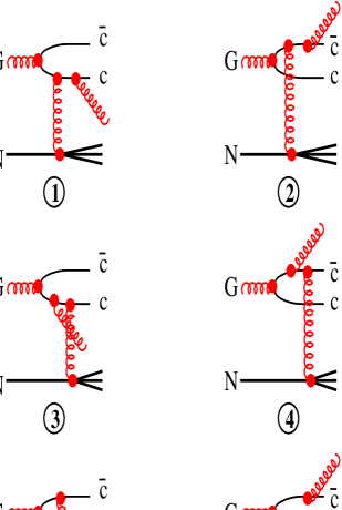
Figure 12: Born graphs contributing to $\bar{c}c$ pair production accompanied with radiation of a gluon. The $\bar{c}c$ is in a color-singlet and C-even state.

Note that the two sets of diagrams, 1-10 and 11-12, are gauge invariant over the t-channel gluon, i.e. the two contribution to the cross section are infra-red stable. However, they correspond to different Fock components of the incident gluon in the light-cone approach. The first set (1-10) corresponds to a fluctuation containing a colorless $\bar{c}c$ and a gluon (see below), white the second one (11-12) describes a fluctuation with a colored $\bar{c}c$ and a gluon. In the latter case the $\bar{c}c$ has to interact with the target to become colorless, in the same way as for the $G\to\bar{c}c$ Fock component considered above in Sect. 3. The gluon does not interact at all at the Born level, therefore these graphs 11-12 do not contribute to gluon shadowing.

The amplitude of a colorless $\bar{c}c$ production corresponding to graphs 1-10 has the following structure,

$$A^{\bar{\mu}\mu}=\sum\limits_{l=1}^{10}A^{\bar{\mu}\mu}_{l}\ ,$$ (D.2)

where

$$A^{\bar{\mu}\mu}_{l}=\frac{i\,\alpha_{s}^{3/2}}{4\sqrt{3}\,D_{l}\,(k_{T}^{2}+\lambda^{2})}\,\sum\limits_{d=1}^{8}f_{abd}\,F^{(d)}_{GN\to X}(k_{T},\{X\})\ \xi^{\mu}_{c}\Bigr{.}^{\dagger}\,\hat{\Gamma}_{l}\,\bar{\xi}^{\bar{\mu}}_{\bar{c}}\ .$$ (D.3)

Here $\lambda$ is the effective gluon mass aimed to incorporate confinement, its value we discuss later. The amplitude $F^{(d)}_{GN\to X}(k_{T},\{X\})$ determines the unintegrated gluon density as it is introduced in (3),

$$\int d\{X\}\sum\limits_{d=1}^{8}\Bigl{|}F^{(d)}_{GN\to X}(k_{T},\{X\})\Bigr{|}^{2}=4\pi\,{\cal F}(k_{T}^{2},x)\ .$$ (D.4)

Here

$$x = \frac{M^{2}(\bar{c},c,G)}{s}\ ;$$ (D.5)

$$M^{2}(\bar{c},c,G) = \frac{m_{c}^{2}+k_{1}^{2}}{\alpha_{1}}+\frac{m_{c}^{2}+k_{2}^{2}}{\alpha_{2}}+\frac{\lambda^{2}+k_{3}^{2}}{\alpha_{3}}\ ,$$ (D.6)

where $\vec{k}_{1},\ \vec{k}_{2},\ \vec{k}_{3}$ and $\alpha_{1},\ \alpha_{2},\ \alpha_{3}$ are the transverse momenta and fractions of the initial light-cone momentum of the projectile gluon carried by the produced $\bar{c},\ c$ and $G$ (see Fig. 12), respectively, and

$$\vec{k}_{T}=\vec{k}_{1}+\vec{k}_{2}+\vec{k}_{3}\ .$$ (D.7)

The $c$-quark spinors $\xi$ are defined in (8); $\{X\}$ is the set of variables describing the state $X$; the 10 vertex functions $\hat{\Gamma}_{l}$ read,

$$\hat{\Gamma}_{1} = \hat{U}_{1}(\vec{k}_{1},\alpha_{1})\,\hat{V}_{1}(\vec{k}_{23},\alpha_{2},\alpha_{3})\ ;$$

$$\hat{\Gamma}_{2} = -\hat{V}_{1}(\vec{k}_{13},\alpha_{1},\alpha_{3})\,\hat{U}_{1}(\vec{k}_{2},\alpha_{2})\,\ ;$$

$$\hat{\Gamma}_{3} = \alpha_{1}\,\hat{U}_{1}(\vec{k}_{1},\alpha_{1})\,\hat{V}_{1}(\vec{k}_{23}-\alpha_{3}\vec{k}_{T},\alpha_{2},\alpha_{3})\ ;$$

$$\hat{\Gamma}_{4} = -\alpha_{2}\,\hat{V}_{2}(\vec{k}_{13}-\alpha_{3}\vec{k}_{T},\alpha_{1},\alpha_{3})\,\hat{U}_{2}(\vec{k}_{2},\alpha_{2})\,\ ;$$

$$\hat{\Gamma}_{5} = \alpha_{2}\alpha_{3}\,\hat{U}_{1}(\vec{k}_{1}-\vec{k}_{T},\alpha_{1})\,\hat{V}_{1}(\vec{k}_{23},\alpha_{2},\alpha_{3})\ ;$$

$$\hat{\Gamma}_{6} = -\alpha_{1}\alpha_{3}\,\hat{V}_{2}(\vec{k}_{13},\alpha_{1},\alpha_{3})\,\hat{U}_{2}(\vec{k}_{2}-\vec{k}_{T},\alpha_{2})\,\ ;$$

$$\hat{\Gamma}_{7} = -2\alpha_{1}\,\hat{U}_{1}(\vec{k}_{1},\alpha_{1})\,\hat{V}_{1}(\vec{k}_{23}+\alpha_{2}\vec{k}_{T},\alpha_{2},\alpha_{3})\ ;$$

$$\hat{\Gamma}_{8} = 2\alpha_{2}\,\hat{V}_{2}(\vec{k}_{13}+\alpha_{1}\vec{k}_{T},\alpha_{1},\alpha_{3})\,\hat{U}_{2}(\vec{k}_{2},\alpha_{2})\,\ ;$$

$$\hat{\Gamma}_{9} = -2\alpha_{2}\alpha_{3}\,\hat{U}_{1}(\vec{k}_{1}-\alpha_{1}\vec{k}_{T},\alpha_{1})\,\hat{V}_{1}(\vec{k}_{23},\alpha_{2},\alpha_{3})\ ;$$

$$\hat{\Gamma}_{10} = 2\alpha_{1}\alpha_{3}\,\hat{V}_{2}(\vec{k}_{13},\alpha_{1},\alpha_{3})\,\hat{U}_{2}(\vec{k}_{2}-\alpha_{2}\vec{k}_{T},\alpha_{2})\ .$$ (D.8)

Here

$$\vec{k}_{13}=\alpha_{3}\vec{k}_{1}-\alpha_{1}\vec{k}_{3}\ ;$$

$$\vec{k}_{23}=\alpha_{3}\vec{k}_{2}-\alpha_{2}\vec{k}_{3}\ ;$$

$$\alpha_{1}+\alpha_{2}+\alpha_{3}=1\ .$$ (D.9)

The matrixes $\hat{U}_{1,2}$ and $\hat{V}_{1,2}$ are defined as follows,

$$\hat{U}_{1}(\vec{k}_{1},\alpha_{1}) = m_{c}\,\vec{\sigma}\cdot\vec{e}+(1-2\alpha_{1})\,\vec{e}\cdot\vec{k}_{1}+i\,(\vec{e}\times\vec{n})\cdot\vec{k}_{1}\ ;$$

$$\hat{U}_{2}(\vec{k}_{2},\alpha_{2}) = m_{c}\,\vec{\sigma}\cdot\vec{e}+(1-2\alpha_{2})\,\vec{e}\cdot\vec{k}_{2}+i\,(\vec{e}\times\vec{n})\cdot\vec{k}_{2}\ ;$$ (D.10)

$$label{d4a}$$ (D.11)

$$\hat{V}_{1}(\vec{k}_{23},\alpha_{2},\alpha_{3}) = (2\alpha_{2}+\alpha_{3})\,\vec{k}_{23}\cdot\vec{e}+i\,m_{c}\,\alpha_{3}^{2}\,(\vec{n}\times\vec{e})\cdot\vec{\sigma}-i\,\alpha_{3}\,(\vec{k}_{23}\times\vec{e})\cdot\vec{\sigma}\ ;$$

$$\hat{V}_{2}(\vec{k}_{13},\alpha_{1},\alpha_{3}) = (2\alpha_{1}+\alpha_{3})\,\vec{k}_{13}\cdot\vec{e}+i\,m_{c}\,\alpha_{3}^{2}\,(\vec{n}\times\vec{e})\cdot\vec{\sigma}-i\,\alpha_{3}\,(\vec{k}_{13}\times\vec{e})\cdot\vec{\sigma}\ .$$

The functions $D_{l}$ in the denominator of (D.3) read,

$$D_{1} = \Delta_{0}(\vec{k}_{1},\alpha_{1})\,\Delta_{2}(\vec{k}_{23},\alpha_{2},\alpha_{3})\ ;$$

$$D_{2} = \Delta_{0}(\vec{k}_{2},\alpha_{2})\,\Delta_{2}(\vec{k}_{13},\alpha_{1},\alpha_{3})\ ;$$

$$D_{3} = \Delta_{0}(\vec{k}_{1},\alpha_{1})\,\Delta_{1}(\vec{k}_{1},\vec{k}_{23}-\alpha_{3}\vec{k}_{T},\alpha_{1},\alpha_{2},\alpha_{3})\ ;$$

$$D_{4} = \Delta_{0}(\vec{k}_{2},\alpha_{2})\,\Delta_{1}(\vec{k}_{2},\vec{k}_{13}-\alpha_{3}\vec{k}_{T},\alpha_{2},\alpha_{1},\alpha_{3})\ ;$$

$$D_{5} = \Delta_{1}(\vec{k}_{1}-\vec{k}_{T},\vec{k}_{23},\alpha_{1},\alpha_{2},\alpha_{3})\,\Delta_{2}(\vec{k}_{23},\alpha_{2},\alpha_{3})\ ;$$

$$D_{6} = \Delta_{1}(\vec{k}_{2}-\vec{k}_{T},\vec{k}_{13},\alpha_{2},\alpha_{1},\alpha_{3})\,\Delta_{2}(\vec{k}_{13},\alpha_{1},\alpha_{3})\ ;$$

$$D_{7} = \Delta_{0}(\vec{k}_{1},\alpha_{1})\,\Delta_{1}(\vec{k}_{1},\vec{k}_{23}+\alpha_{2}\vec{k}_{T},\alpha_{1},\alpha_{2},\alpha_{3})\ ;$$

$$D_{8} = \Delta_{0}(\vec{k}_{2},\alpha_{2})\,\Delta_{1}(\vec{k}_{2},\vec{k}_{13}+\alpha_{1}\vec{k}_{T},\alpha_{2},\alpha_{1},\alpha_{3})\ ;$$

$$D_{9} = \Delta_{2}(\vec{k}_{23},\alpha_{2},\alpha_{3})\,\Delta_{1}(\vec{k}_{1}-\alpha_{1}\vec{k}_{T},\vec{k}_{23},\alpha_{1},\alpha_{2},\alpha_{3})\ ;$$

$$D_{10} = \Delta_{2}(\vec{k}_{13},\alpha_{1},\alpha_{3})\,\Delta_{1}(\vec{k}_{2}-\alpha_{2}\vec{k}_{T},\vec{k}_{13},\alpha_{2},\alpha_{1},\alpha_{3})\ ,$$ (D.13)

where

$$\Delta_{0}(\vec{k}_{1},\alpha_{1}) = m_{c}^{2}+k_{1}^{2}-\alpha_{1}(1-\alpha_{1})\,\lambda^{2}\ ;$$

$$\Delta_{2}(\vec{k}_{13},\alpha_{1},\alpha_{3}) = \alpha_{3}^{3}\,m_{c}^{2}+\alpha_{1}(\alpha_{1}+\alpha_{3})\,\lambda^{2}+k_{13}^{2}\ ;$$

$$\Delta_{1}(\vec{k}_{1},\vec{k}_{23},\alpha_{1},\alpha_{2},\alpha_{3}) = (\alpha_{1}-\alpha_{3})(\alpha_{3}\,m_{c}^{2}+\alpha_{1}\alpha_{2}\,\lambda^{2})+\alpha_{1}k_{23}^{2}+\alpha_{2}\alpha_{2}\,k_{1}^{2}\ .$$ (D.14)

Functions $\Delta_{0}$, $\Delta_{1}$ and $\Delta_{2}$ are not independent, but satisfy the relation

$$\Bigl{[}\Delta_{0}(\vec{k}_{1},\alpha_{1})\,\Delta_{2}(\vec{k}_{23},\alpha_{2},\alpha_{3})\Bigr{]}^{-1}=\alpha_{1}\,\Bigl{[}\Delta_{0}(\vec{k}_{1},\alpha_{1})\,\Delta_{1}(\vec{k}_{1},\vec{k}_{23},\alpha_{1},\alpha_{2},\alpha_{3})\Bigr{]}^{-1}$$ (D.15)

$$+ \alpha_{2}\alpha_{3}\,\Bigl{[}\Delta_{2}(\vec{k}_{23},\alpha_{2},\alpha_{3})\,\Delta_{1}(\vec{k}_{1},\vec{k}_{23},\alpha_{1},\alpha_{2},\alpha_{3})\Bigr{]}^{-1}\ .$$

The sum of ten amplitudes Eq. (D.3) is convenient to split up to four terms,

$$\hat{M}=\sum\limits_{l=1}^{10}=\sum\limits_{i=1}^{4}\hat{M}_{i}\,\frac{\hat{\Gamma}_{l}}{D_{l}}\ ,$$ (D.16)

which can be represented using relation (D.15) in the following form,

$$\hat{M}_{1} = \alpha_{1}\,\hat{\nu}_{1}(\vec{k}_{1},\alpha_{1})\,\Bigr{[}\hat{\mu}_{1}(\vec{k}_{1},\vec{k}_{23},\alpha_{1},\alpha_{2},\alpha_{3})+\hat{\mu}_{1}(\vec{k}_{1},\vec{k}_{23}-\alpha_{3}\vec{k}_{T},\alpha_{1},\alpha_{2},\alpha_{3})$$ (D.17)

$$- 2\,\hat{\mu}_{1}(\vec{k}_{1},\vec{k}_{23}+\alpha_{2}\vec{k}_{T},\alpha_{1},\alpha_{2},\alpha_{3})\Bigr{]}$$

$$\hat{M}_{2} = -\alpha_{2}\,\Bigl{[}\hat{\mu}_{2}(\vec{k}_{2},\vec{k}_{13},\alpha_{2},\alpha_{1},\alpha_{3})+\hat{\mu}_{2}(\vec{k}_{2},\vec{k}_{13}-\alpha_{3}\vec{k}_{T},\alpha_{1},\alpha_{2},\alpha_{3})$$ (D.18)

$$- 2\hat{\mu}_{2}(\vec{k}_{2},\vec{k}_{13}+\alpha_{1}\vec{k}_{T},\alpha_{1},\alpha_{2},\alpha_{3})\Bigr{]}\,\nu_{2}(\vec{k}_{2},\alpha_{2})\ ;$$

$$\hat{M}_{3} = \alpha_{2}\alpha_{3}\,\Bigr{[}\hat{\lambda}_{1}(\vec{k}_{1},\vec{k}_{23},\alpha_{1},\alpha_{2},\alpha_{3})+\hat{\lambda}_{1}(\vec{k}_{1}-\vec{k}_{T},\vec{k}_{23},\alpha_{1},\alpha_{2},\alpha_{3})$$ (D.19)

$$- 2\hat{\lambda}_{1}(\vec{k}_{1}-\alpha_{1}\vec{k}_{T},\vec{k}_{23},\alpha_{1},\alpha_{2},\alpha_{3})\Bigr{]}\,\hat{\rho}_{1}(\vec{k}_{23},\alpha_{2},\alpha_{3})\ ;$$

$$\hat{M}_{4} = -\alpha_{1}\alpha_{2}\,\hat{\rho}_{2}(\vec{k}_{13},\alpha_{1},\alpha_{3})\,\Bigl{[}\hat{\lambda}_{2}(\vec{k}_{2},\vec{k}_{13},\alpha_{1},\alpha_{2},\alpha_{3})$$ (D.20)

$$+ \hat{\lambda}_{2}(\vec{k}_{2}-\vec{k}_{T},\vec{k}_{13},\alpha_{1},\alpha_{2},\alpha_{3})-2\hat{\lambda}_{2}(\vec{k}_{2}-\alpha_{2}\vec{k}_{T},\vec{k}_{13},\alpha_{1},\alpha_{2},\alpha_{3})\Bigr{]}\ .$$

The following notations are used here,

$$\hat{\nu}_{1}(\vec{k}_{1},\alpha_{1}) = \frac{\hat{U}_{1}(\vec{k}_{1},\alpha_{1})}{\Delta_{0}(\vec{k}_{1},\alpha_{1})}\ ;$$

$$\hat{\nu}_{2}(\vec{k}_{2},\alpha_{2}) = \frac{\hat{U}_{2}(\vec{k}_{2},\alpha_{2})}{\Delta_{0}(\vec{k}_{2},\alpha_{2})}\ ;$$ (D.21)

$$\hat{\mu}_{1}(\vec{k}_{1},\vec{k}_{23},\alpha_{1},\alpha_{2},\alpha_{3}) = \frac{\hat{V}_{1}(\vec{k}_{23},\alpha_{2},\alpha_{3})}{\Delta_{1}(\vec{k}_{1},\vec{k}_{23},\alpha_{1},\alpha_{2},\alpha_{3})}\ ;$$

$$\hat{\mu}_{2}(\vec{k}_{2},\vec{k}_{13},\alpha_{1},\alpha_{2},\alpha_{3}) = \frac{\hat{V}_{2}(\vec{k}_{13},\alpha_{1},\alpha_{3})}{\Delta_{1}(\vec{k}_{2},\vec{k}_{13},\alpha_{1},\alpha_{2},\alpha_{3})}\ ;$$ (D.22)

$$\hat{\lambda}_{1}(\vec{k}_{1},\vec{k}_{23},\alpha_{1},\alpha_{2},\alpha_{3}) = \frac{\hat{U}_{1}(\vec{k}_{1},\alpha_{1})}{\Delta_{1}(\vec{k}_{1},\vec{k}_{23},\alpha_{1},\alpha_{2},\alpha_{3})}\ ;$$

$$\hat{\lambda}_{2}(\vec{k}_{2},\vec{k}_{13},\alpha_{1},\alpha_{2},\alpha_{3}) = \frac{\hat{U}_{2}(\vec{k}_{2},\alpha_{2})}{\Delta_{1}(\vec{k}_{2},\vec{k}_{13},\alpha_{1},\alpha_{2},\alpha_{3})}\ ;$$ (D.23)

$$\hat{\rho}_{1}(\vec{k}_{23},\alpha_{2},\alpha_{3}) = \frac{\hat{V}_{1}(\vec{k}_{23},\alpha_{2},\alpha_{3})}{\Delta_{2}(\vec{k}_{23},\alpha_{2},\alpha_{3})}\ ;$$

$$\hat{\rho}_{2}(\vec{k}_{13},\alpha_{1},\alpha_{3}) = \frac{\hat{V}_{2}(\vec{k}_{13},\alpha_{1},\alpha_{3})}{\Delta_{2}(\vec{k}_{13},\alpha_{1},\alpha_{3})}\ ;$$ (D.24)

Apparently, the amplitude operators in Eqs. (D.17)-(D.20) vanish, $\hat{M}_{i}\to 0$ when $\vec{k}_{T}\to 0$ what guarantees infra-red stability of the cross section of gluon radiation.

Since the cross section steeply falls down at large $k_{T}^{2}$ and $\hat{M}_{i}(k_{T}=0)=0$ we can expand the amplitudes at small $k_{T}$,

$$M_{i}(k_{T})\approx\vec{k}_{T}\left[\frac{\partial}{\partial\vec{k}_{T}}\,\hat{M}_{i}(\vec{k}_{T})\right]_{k_{T}=0}\ .$$ (D.25)

Using Eqs. (D.17)-(D.20) we find,

$$\left.\frac{\partial\hat{M}_{1}}{\partial\vec{k}_{T}}\right|_{k_{T}=0} \approx -\alpha_{1}\,\hat{\nu}_{1}\,\frac{\partial\hat{\mu}_{1}}{\partial\vec{k}_{23}}\,(\alpha_{3}+2\,\alpha_{2})\ ;$$ (D.26)

$$\left.\frac{\partial\hat{M}_{2}}{\partial\vec{k}_{T}}\right|_{k_{T}=0} \approx \alpha_{1}\,\frac{\partial\hat{\mu}_{2}}{\partial\vec{k}_{13}}\,\hat{\nu}_{2}\,(\alpha_{3}+2\,\alpha_{1})\ ;$$ (D.27)

$$\left.\frac{\partial\hat{M}_{3}}{\partial\vec{k}_{T}}\right|_{k_{T}=0} \approx -\alpha_{2}\alpha_{3}\,\frac{\partial\hat{\lambda}_{1}}{\partial\vec{k}_{2}}\,\hat{\rho}_{1}\,(1-2\,\alpha_{1})\ ;$$ (D.28)

$$\left.\frac{\partial\hat{M}_{4}}{\partial\vec{k}_{T}}\right|_{k_{T}=0} \approx \alpha_{1}\alpha_{3}\,\hat{\rho}_{2}\,\frac{\partial\hat{\lambda}_{2}}{\partial\vec{k}_{2}}\,(1-2\,\alpha_{2})\ .$$ (D.29)

Using the obvious relations

$$1-2\alpha_{1} = \alpha_{2}-\alpha_{1}+\alpha_{3}\ ,$$

$$1-2\alpha_{2} = \alpha_{1}-\alpha_{2}+\alpha_{3}\ ,$$ (D.30)

we conclude that the terms $\hat{M}_{3}$ and $\hat{M}_{4}$ in the amplitude of $\bar{c}c$ pair production are negligible compared to $\hat{M}_{1}$ and $\hat{M}_{2}$. Indeed, since the $\bar{c}c$ must be projected on the wave function of the heavy charmonium, one can make use of the fact that it is a nonrelativistic system, and that the radiated gluon is predominantly soft, i.e.

$$|\vec{k}_{1}-\vec{k}_{2}| \ll m_{c}\ ,$$

$$|\alpha_{1}-\alpha_{2}| \ll 1\ ,$$

$$\alpha_{3} \ll 1\ .$$ (D.31)

These conditions also help to simplify essentially the Eqs. (D.26) and (D.29) for $\hat{M}_{1}$ and $\hat{M}_{2}$. First of all, for vanishing $\alpha_{3}$ one can neglect the terms containing the Pauli matrixes in the definition (LABEL:d4b) of $\hat{V}_{1}$ and $\hat{V}_{2}$ which now commutate with $\hat{U}_{1}$ and $\hat{U}_{2}$.

Further, for small $\alpha_{3}$ Eq. (D.9) leads to $\vec{k}_{13}\approx-\alpha_{1}\,\vec{k}_{3}$, $\vec{k}_{23}\approx-\alpha_{2}\,\vec{k}_{3}$. Since from (D.31) it follows that $\alpha_{1}\approx\alpha_{2}\approx 1/2$ eventually we arrive at $\vec{k}_{13}\approx\vec{k}_{23}\approx-\vec{k}_{3}/2$. Then the propagator $\Delta_{1}$ can be represented as

$$\Delta_{1} = {1\over 8}\,(k_{3}^{2}+\tau^{2})+O[\alpha_{3}(\vec{k}_{1}-\vec{k}_{2})]\ ;$$

$$\tau^{2} = \lambda^{2}+\alpha_{3}\,M^{2}\ ;$$

$$M = 2m_{c}\approx M_{\bar{c}c}\ .$$ (D.32)

The approximations done we arrive to a simplified form of the amplitude,

$$\hat{M} = 2\,\left[\frac{m_{c}\,\vec{\sigma}\cdot\vec{e}+i\,(\vec{n}\times\vec{k}_{1})\cdot\vec{e}}{m_{c}^{2}+k_{1}^{2}}-\frac{m_{c}\,\vec{\sigma}\cdot\vec{e}i\,(\vec{n}\times\vec{k}_{2})\cdot\vec{e}}{m_{c}^{2}+k_{2}^{2}}\right]$$ (D.33)

$$\times \left[\frac{2(\vec{k}_{3}-\vec{k}_{T})\cdot\vec{e}}{(\vec{k}_{3}-\vec{k}_{T})^{2}+\tau^{2}}-\frac{2\,\vec{k}_{3}\cdot\vec{e}}{k_{3}^{2}+\tau^{2}}\right]\ .$$

Here we suppressed in the propagator the term $\lambda^{2}/4\sim\Lambda_{QCD}^{2}/4$ which is tiny compared to $m_{c}^{2}$.

Using Eq. (D.33) the amplitude (D.3) takes the form

$$A^{\bar{\mu}\mu}_{ab}(\vec{k}_{12},\vec{k}_{3},\vec{k}_{T},\alpha_{3})=\int d^{2}b\,d^{2}s\,d^{2}r\,A^{\bar{\mu}\mu}_{ab}(\vec{b},\vec{s},\vec{r},\alpha_{3})\exp\Bigl{[}i(\vec{b}\cdot\vec{k}_{T}+\vec{s}\cdot\vec{k}_{3}+\vec{r}\cdot\vec{k}_{12}\Bigr{]}\ ,$$ (D.34)

where

$$A^{\bar{\mu}\mu}_{ab}(\vec{b},\vec{s},\vec{r},\alpha_{3})\ =\ \frac{i\,\sqrt{3}}{2}\,\sum\limits_{d=1}^{8}f_{abd}\,\Phi^{\bar{\mu}\mu}_{G}(\vec{r},\alpha=1/2)$$ (D.35)

$$\times \,\left\{\Phi_{qG}\left(\vec{s}+\frac{\vec{r}}{2}\right)\,\left[\gamma^{(d)}\Bigl{(}\vec{b}+\vec{s},\{X\}\Bigr{)}-\gamma^{(d)}\Bigl{(}\vec{b}-\frac{\vec{r}}{2},\{X\}\Bigr{)}\right]\right.$$

$$- \left.\Phi_{qG}\left(\vec{s}-\frac{\vec{r}}{2}\right)\,\left[\gamma^{(d)}\Bigl{(}\vec{b}+\vec{s},\{X\}\Bigr{)}-\gamma^{(d)}\Bigl{(}\vec{b}+\frac{\vec{r}}{2},\{X\}\Bigr{)}\right]\right\}\ .$$

Here $\Phi^{\bar{\mu}\mu}_{G}(\vec{r},\alpha)$ is the distribution amplitude for a $\bar{c}c$ fluctuation of a gluon given by Eq. (7), and $\Phi_{qG}(\vec{s})$ is the distribution amplitude for a quark-gluon fluctuation of a quark which has the form,

$$\Phi_{qG}(\vec{r})=\frac{2i}{\pi}\,\sqrt{\frac{\alpha_{s}}{3}}\,\vec{e}\cdot\vec{\nabla}_{r}\,K_{0}(\tau r)\ .$$ (D.36)

The profile function $\gamma^{(d)}(\vec{b},\{X\})$ in Eq. (D.35) is related to the amplitude $F^{(d)}(\vec{k}_{T},\{X\})$ by Fourier transform,

$$\gamma^{(d)}(\vec{b},\{X\})=\frac{\sqrt{\alpha_{s}}}{2\pi\sqrt{6}}\int\frac{d^{2}k_{T}}{k_{T}^{2}+\lambda^{2}}\,e^{-i\vec{k}_{T}\cdot\vec{b}}\,F^{(d)}_{GN\to X}(\vec{k}_{T},\{X\})\ .$$ (D.37)

This profile function is related to the unintegrated gluon density ${\cal F}(k_{T},x)$ and the dipole cross section $\sigma_{\bar{q}q}(r,x)$ by the relation,

$$\int d^{2}b\,d\Gamma_{X}\,\sum\limits_{d=1}^{8}\left|\gamma^{(d)}(\vec{b}+\vec{r},\{X\})-\gamma^{(d)}(\vec{b},\{X\})\right|^{2}$$ (D.38)

$$= \frac{4\pi}{3}\,\alpha_{s}\,\int\frac{d^{2}k_{T}}{k_{T}^{2}+\lambda^{2}}\,\left(1-e^{i\vec{k}_{T}\cdot\vec{r}}\right)\,{\cal F}(k_{T},x)=\sigma_{\bar{q}q}(r,x)\ .$$

Now we can calculate the amplitude of $\chi$ production accompanied by gluon radiation which corresponds to the graphs depicted in Fig. 12 with the $\bar{c}c$ pair projected to the wave function of $\chi$,

$$A^{\chi}_{ab}(\vec{k}_{T},\vec{k}_{3})=\sum\limits_{\bar{\mu}\mu}\,\int d\alpha\,d^{2}b\,d^{2}s\,d^{2}r\,\Phi_{\chi}^{\bar{\mu}\mu}(\vec{r},\alpha)\,A^{\bar{\mu}\mu}_{ab}(\vec{b},\vec{s},\vec{r})\,\exp\left[i(\vec{b}\cdot\vec{k}_{T}+\vec{s}\cdot\vec{k}_{3})\right]\ .$$ (D.39)

Note that the typical value of $r\sim 1/m_{c}$ is much smaller than the mean separation $b\sim 1/\Lambda_{QCD}$. Therefore, we can use the approximation $\gamma^{(d)}(\vec{b}\pm\vec{r},\{X\})\approx\gamma^{(d)}(\vec{b},\{X\})$ in Eq. (D.35), then the amplitude $A^{\bar{\mu}\mu}$ takes the form which is known for the radiation of a heavy photon by a quark, i.e. the amplitude of Drell-Yan process [26, 28],

$$A^{\chi}_{ab}(\vec{k}_{T},\vec{k}_{3},\alpha_{3}) \approx -\frac{i\sqrt{3}}{2}\,\sum\limits_{\bar{\mu}\mu}\,\int d^{2}b\,d^{2}s\,\Psi(s,\alpha_{3})\,\exp\left[i(\vec{b}\cdot\vec{k}_{T}+\vec{s}\cdot\vec{k}_{3})\right]$$ (D.40)

$$\times \left[\gamma^{(d)}\Bigl{(}\vec{b}+\vec{s},\{X\}\Bigr{)}-\gamma^{(d)}\Bigl{(}\vec{b},\{X\}\Bigr{)}\right]\ ,$$

where $\Psi(s,\alpha_{3})$ defined in (50) is the effective distribution amplitude for s $\chi-G$ fluctuation of a gluon, which is the analog for the $\gamma^{*}\,q$ fluctuation of a quark.

The two terms in square brackets in (D.40) correspond to the two diagrams in Fig. 6 which are the same as for Drell-Yan reaction if to replace the virtual photon by $\chi$ and the incoming and recoil quarks by gluons. Therefore, it is natural to expect the corresponding cross section to have the same factorized form as for Drell-Yan reaction. Indeed, squaring expression Eq. (D.40) and using Eq. (D.38) we arrive at the expression Eq. (49) for the cross section.

References

• [1] The NA3 Collaboration, J. Badier et al., Z. Phys. C20 (1983) 101
• [2] The E537 Coll., S. Katsanevas et al., Phys. Rev. Lett., 60 (1988) 2121
• [3] The E866 Collaboration, M.J. Leitch et al., Phys. Rev. Lett. 84 (2000) 3256
• [4] The NA38 Collaboration, C. Baglin et al., Phys. Lett. B345 (1995) 617
• [5] The NA50 Collaboration, M.C. Abreu et al., Phys. Lett. B477 (2000) 28
• [6] B.Z. Kopeliovich, A. Schäfer and A.V. Tarasov, Phys. Rev. D62 (2000) 054022
• [7] M. Vaenttinen, P. Hoyer, S.J. Brodsky and W.-K. Tang, Phys. Rev.D51 (1995) 3332
• [8] E.L. Berger and D. Jones, Phys. Rev. D23 (1981) 1521
• [9] W.-K. Tang and M. Vaenttinen, Phys. Rev. D54 (1996) 4349
• [10] Ph. Hagler, R. Kirshner, A. Shäfer, L. Szymanowski and A.O. Teryaev, Phys. Rev. D63 (2001) 077501
• [11] S.J. Brodsky and A.H. Mueller, Phys. Lett. B206 (1988) 685
• [12] The E772 Collaboration, D.M. Alde et al, Phys. Rev. Lett. 64 (1990) 2479.
• [13] B.Z. Kopeliovich and B.G. Zakharov, Phys. Rev. D44 (1991) 3466.
• [14] O. Benhar, B.Z. Kopeliovich, Ch. Mariotti, N.N. Nikolaev and B.G. Zakharov, Phys. Rev. Lett. 69 (1992) 1156.
• [15] J. Hüfner and B.Z. Kopeliovich, Phys. Rev. Lett. 76 (1996) 192
• [16] D. Kharzeev and H. Satz, Phys. Lett. B356 (1995) 365
• [17] The NMC Collaboration, Ch. Mariotti et al., Phys. Lett. B332 (1994) 195
• [18] The HERMES Collaboration, K. Ackerstaff et al., Phys. Rev. Lett. 82 (1999) 3025
• [19] J. Hüfner, B.Z. Kopeliovich and J. Nemchik, Phys. Lett. B383 (1996) 362
• [20] K. Boreskov, A. Capella, A. Kaidalov and J. Tran Thanh Van, Phys. Rev. D47 (1993) 919
• [21] B.Z. Kopeliovich, Dynamics and Phenomenology of Charmonium Production off Nuclei, in proc. of the Workshop Hirschegg’97: QCD Phase Transitions’, Hirschegg, Austria, January, 1997, ed. by H. Feldmeier, J. Knoll, W. Nörenberg and J. Wambach, Darmstadt, 1997, p. 281; hep-ph/9702365
• [22] J. Hüfner, Yu.P. Ivanov, B.Z. Kopeliovich and A.V. Tarasov, Phys. Rev. D62 (2000) 094022
• [23] B.Z. Kopeliovich and F. Niedermayer, Nuclear screening in $J/\Psi$ and Drell-Yan pair production, JINR-E2-84-834, Dubna 1984, see the scanned version in KEK library:
http://www-lib.kek.jp/cgi-bin/img_index?8504113
• [24] M.B. Johnson et al., Phys. Rev. Lett. 86 (2001) 4483
• [25] M.B. Johnson et al., Energy Loss versus Shadowing in Drell-Yan Reaction on Nuclei, paper in preparation
• [26] B.Z. Kopeliovich, Soft Component of Hard Reactions and Nuclear Shadowing (DIS, Drell-Yan reaction, heavy quark production), in proc. of the Workshop Hirschegg’95: Dynamical Properties of Hadrons in Nuclear Matter, Hirschegg, January, 1995, ed. by H. Feldmeier and W. Nörenberg, Darmstadt, 1995, p. 102 (hep-ph/9609385)
• [27] S.J. Brodsky, A. Hebecker and E. Quack, Phys. Rev. D55 (1997) 2584
• [28] B.Z. Kopeliovich, A. Schäfer and A.V. Tarasov, Phys. Rev. C59 (1999) 1609 (extended version in hep-ph/9808378)
• [29] B.Z. Kopeliovich, J. Raufeisen and A.V. Tarasov, Phys. Lett. B503 (2001) 91
• [30] A.B. Zamolodchikov, B.Z. Kopeliovich and L.I. Lapidus, Sov. Phys. JETP Lett. 33 (1981) 612
• [31] V.B. Berestetski, E.M. Lifshitz, and L.P. Pitaevski, Relativistic Quantum Theory. Clarendon Press, Oxford, 1971.
• [32] C. Gerschel and J. Hüfner, Phys. Lett. B207 (1988) 253
• [33] B.Z. Kopeliovich and Al.B. Zamolodchikov, unpublished. See in: B. Z. Kopeliovich and L. I. Lapidus, Colour Exchange of High Energy Hadrons in Nuclei, Proc. of the VI Balaton Conf. on Nucl. Phys., p.103, Balatonfüred, Hungary, 1983
• [34] N.N. Nikolaev, G. Piller and B.G. Zakharov, J. Exp. Theor. Phys. 81 (1995) 851
• [35] J. Hüfner, B.Z. Kopeliovich and Al.B. Zamolodchikov, Z. Phys. A357 (1997) 113
• [36] B.Z. Kopeliovich, J. Raufeisen and A.V. Tarasov, Phys. Lett. B440 (1998) 151
• [37] B.G. Zakharov, Phys.Atom.Nucl. 61 (1998) 838
• [38] K.J. Eskola, V.J. Kolhinen, and P.V. Ruuskanen, Nucl. Phys. B535 (1998) 351
• [39] O.V. Kancheli, Sov. Phys. JETP Lett. 18 (1973) 274
• [40] L.V. Gribov, E.M. Levin and M.G. Ryskin, Nucl. Phys. B188 (1981) 555; Phys. Rep. 100 (1983) 1.
• [41] B.Z. Kopeliovich, J. Raufeisen and A.V. Tarasov, Phys. Rev. C62 (2000) 035204.
• [42] A.H. Mueller, Nucl. Phys. B335 (1990) 115; ibid B558 (1999) 285
• [43] V.N. Gribov, Sov. Phys. JETP 29 (1969) 483; 30 (1970) 709
• [44] L.Frankfurt, M.Strikman, Eur.Phys.J. A5 (1999) 293
• [45] T. Gousset and H.J. Pirner, Phys. Lett. B375 (1996) 349
• [46] B.Z. Kopeliovich and F. Niedermayer, Sov. J. Nucl. Phys. 42 (1985) 797
• [47] F. Niedermayer, Phys. Rev. D34 (1986) 3494
• [48] S.J. Brodsky and P. Hoyer, Phys. Lett. 298B (1993) 165.
• [49] B.Z. Kopeliovich, I.K. Potashnikova, B. Povh and E. Predazzi, Phys. Rev. Lett. 85 (2000) 507
• [50] R. Baier, Yu.L. Dokshitzer, A.H. Mueller, S. Peigne and D. Schiff, Nucl. Phys. B483 (1997) 291; B484 (1997) 265.
• [51] R. Baier, D. Schiff and B.G Zakharov, Energy loss in perturbative QCD, hep-ph/0002198
• [52] P.L. McGaughey, J.M. Moss, J.C. Peng, Ann. Rev. Nucl. Part. Sci. 49 (1999) 217
• [53] The NA38 Collaboration, C. Baglin et al., Phys. Lett. B270 (1991) 105
• [54] M.V.Terent’ev, Sov.J. Nucl. Phys. 24 (1976) 106
• [55] P. Hoyer and S. Peigné, Phys. Rev. D61 (2000) 031501(R)
• [56] A. Martin, Phys. Lett. B93 (1980) 338.
• [57] F. Arleo, P.-B. Gossiaux, J. Aichelin, Charmonium suppression in p-A collisions at RHIC, hep-ph/0105047
• [58] F. Arleo, P.-B. Gossiaux, T. Gousset, J. Aichelin, Phys. Rev. C61 (2000) 054906; Energy loss and $x_{2}$ scaling breakdown in $J/\psi$ nuclear production, hep-ph/0005230