Astroparticle physics signals beyond the Standard Model

Chapter 1 Introduction

The Standard Model (SM) of particle physics is in perfect agreement with all present accelerator experiments . There are, however, signals that point beyond the SM. These can be either theoretical or experimental indications. On the theoretical side one could mention the problems the SM suffers from: too many parameters, triviality of the Higgs sector, Landau-pole in the U(1) sector, etc. On the experimental side there are only indirect signals. In my thesis I will deal with two such indications.

The first one is the presence of baryonic matter around us. The SM seems to provide a mechanism for producing nonzero baryon number starting from symmetric initial conditions. This requires a strong first order finite temperature electroweak phase transition. However, it turned out that for a first order phase transition the mass of the Higgs particle has to be less then $72$ GeV above which only a rapid cross-over can be seen. Since the experimental lower bound on the Higgs boson mass is much higher, SM baryogenesis is ruled out. In order to avoid the conclusion that the present baryon number was simply an initial condition we need to go beyond the Standard Model. The most attractive extension of the SM is the Minimal Supersymmetric Standard Model (MSSM). In the next chapter I will investigate the possibility of baryogenesis in the MSSM.

The second signal that I discuss in my thesis comes from the observed cosmic rays. The highest energy detected cosmic ray events have macroscopic energy, more than $10^{20}$ eV. It is unlikely that these particles were accelerated from lower energies to such a high energy. A more attractive possibility is that they are the decay products of some metastable superheavy particle, usually associated with some Grand Unified Theory (GUT). This appealing possibility clearly points far beyond the SM. In the third chapter of this thesis I give predictions on the density and energy scale of the Ultrahigh energy cosmic ray sources.

The MSSM baryogenesis calculations needed lattice simulations of the bosonic sector of MSSM. This requires a large amount of CPU time. For this purpose a PC based supercomputer was built at the Eötvös University. In the fourth chapter I will discuss the hardware and software architecture of this machine.

In the MSSM project I worked together with Ferenc Csikor, Zoltán Fodor Pál Hegedüs, Tamás Herpay, Antal Jakovác and Attila Piróth. The UHECR calculations were done together with Zoltán Fodor while in the supercomputer project Ferenc Csikor, Zoltán Fodor, Pál Hegedüs, Viktor Horváth and Attila Piróth were also involved. This also means that only a part of the results belong to me. My contribution is the following:

• Writing a 5000 line C program for the MSSM lattice simulations; Development of the heatbath and overrelaxation algorithms for the Higgs and squark fields.

• Performing finite temperature simulations to determine the critical point of the Electroweak Phase Transition and then zero temperature simulations to measure the mass spectrum.

• Determining the phase diagram of MSSM in the $m_{U}^{2}$–$T$ plane in the infinite volume limit. Finding the bubble wall profile during the phase transition and measuring the width of the wall and the change of the ratio of the two Higgs expectation values.

• Determining the density of ultrahigh energy cosmic ray sources based on the clustering features of observations.

• Finding the $P(r,E,E_{c})$ function which gives the probability that a particle produced with energy $E$ is detected above the energy $E_{c}$ after propagation over a distance $r$.

• Determining the fragmentation function of the proton at high energies.

• Finding the mass of the superheavy particle that could be the source of ultrahigh energy cosmic rays.

• Writing the job management system and the kernel driver for the communication cards of the PMS supercomputer.

In my thesis I will concentrate on these aspects of the problems. I have four publications connected to my thesis:

• F. Csikor, Z. Fodor, P. Hegedüs, A. Jakovác, S. D. Katz and A. Piróth, Phys. Rev. Lett. 85, 932 (2000).

• Z. Fodor and S. D. Katz, Phys. Rev. D 63, 023002 (2001).

• Z. Fodor and S. D. Katz, Phys. Rev. Lett. 86, 3224 (2001).

• F. Csikor, Z. Fodor, P. Hegedüs, V. K. Horváth, S. D. Katz and A. Piróth, Comput. Phys. Commun. 134, 139 (2001).

The structure of this thesis is as follows. In chapter 2 I briefly discuss the possibilities of electroweak baryogenesis in the SM and MSSM. Then I present the methods used for lattice simulations of the bosonic sector of MSSM and give the results of finite and zero temperature simulations. The last two sections of this chapter deal with the phase diagram of MSSM and the profile of the bubble wall during the phase transition.

Chapter 3 deals with ultrahigh energy cosmic rays. After a short introduction the density of sources is determined. The interesting assumption that the sources of these cosmic rays can be superheavy particles is discussed in section 3.2.

In chapter 4 the PMS supercomputer is described. Both the hardware and sofware architectures are discussed in detail and results for the performance are also given.

Chapter 2 MSSM Baryogenesis

2.1 Baryogenesis in the Standard Model

The world around us is made up of baryonic matter. This fact can be verified by observations in our vicinity. For distant regions of the Universe we have only indirect signals. If in some distant segment of the Universe anti-world domains existed, the annihilation at the world – anti-world domain walls should affect the diffuse cosmic gamma-ray background. The observed gamma-ray spectrum does not seem to support the possibility of anti-world domains [2].

The observed asymmetry can either be accepted as an initial condition at the ”Big-Bang” or explained by some symmetry breaking mechanism during the evolution of the Universe. While the first solution is rather simple, the second one gives a real challenge to particle physics. The final non-vanishing baryon number of the universe should be derived from symmetric initial conditions.

Every baryogenesis scenario should fulfill three conditions first stated by Sakharov [3]:

1. Baryon number violation

2. C and CP violation

3. Departure from thermal equilibrium

The Standard Model provides an appealing mechanism for baryogenesis. All three conditions are satisfied at high temperatures (around 100 GeV) where the electroweak phase transition (EWPT) takes place. Transitions between the different vacua of the system, called sphalerons, can change the baryon number, $B$. The sphalerons, however, do not only change $B$ but also the lepton number $L$ such that $B-L$ remains constant. This way a $B+L$ asymmetry can be generated. The EWPT is the last possibility during the evolution of the Universe when the baryon number could be generated [4]. In my thesis I will discuss the possibility of electroweak baryogenesis.

Even if during the EWPT all Sakharov conditions are satisfied it does not still mean that the required baryon number will be generated. If the sphaleron rate is too high all generated $B+L$ asymmetry will be washed out. The expansion rate of the universe should be large enough to prevent this. This condition can be formulated using the expectation value of the Higgs field ($v$) in the symmetry-broken phase and the critical temperature ($T_{c}$) of the phase transition:

$$\frac{v}{T_{c}}>1$$ (2.1)

The forthcoming part of this chapter will deal with this condition.

The first detailed description of the EWPT in the SM was based on perturbative techniques [5]. However, there were ${\cal O}(100\%)$ corrections between different orders of the perturbative expansion for Higgs boson masses larger than about 60 GeV. This questions the use of perturbation theory in this region. The dimensionally reduced 3d effective model (e.g. [6]) was also studied perturbatively and it gave similar conclusions. To solve the problem of higher Higgs masses lattice simulations were needed. Both direct four dimensional simulations [7, 8] and reduced three dimensional simulations [9] were carried out. The results are in agreement and they contradict perturbation theory. While perturbation theory predicts a first order phase transition even for large Higgs masses, lattice studies show that the strength of the transition gets weaker and there is an endpoint [10, 11] at Higgs mass $m_{H}=72\pm 1.4$ GeV [11].

The present experimental lower limit of the SM Higgs boson mass is by several standard deviations larger than the endpoint value. Thus any EWPT in the SM is excluded. This also means that the SM baryogenesis in the early Universe is ruled out.

2.2 Baryogenesis in the MSSM

In order to explain the observed baryon asymmetry, extended versions of the SM are necessary. Clearly, the most attractive possibility is MSSM. According to perturbative predictions the strength of the EWPT in the MSSM depends strongly on the scalar masses [12]. Since now there are more scalars than the Higgs itself they can be used to increase the Higgs mass while keeping $v/T_{c}$ above $1$. In particular if the stop mass is smaller than the top mass then baryogenesis may be possible even for Higgs masses around 100 GeV [13]. At two-loop level stop-gluon graphs give a considerable strengthening of the EWPT (e.g. third and fourth paper of [12]).

A reduced 3d version of the MSSM has recently been studied on the lattice [14]. It included ${\mathrm{SU(3)}}\!\times\!{\mathrm{SU(2)}}$ gauge fields, the right-handed stop and a “light” combination of the Higgses. The results show that the EWPT can be strong enough, i.e. $v/T_{c}\!>\!1$, up to $m_{h}\!\approx\!105$ GeV and $m_{\tilde{t}}\!\approx\!165$ GeV, where $m_{h}$ is the mass of the lightest neutral scalar and $m_{\tilde{t}}$ is that of the stop squark.

In this chapter I study the EWPT in the MSSM on four dimensional lattices. Lattice simulation of fermionic fields is extremely CPU consuming. Fortunately all problems arising in the perturbative approach come from the bosonic sector of the theory. Thus we can find a mixed solution: simulating only the bosonic sector on the lattice, and taking fermions into account perturbatively [16]. In fact the method we used is to study almost the whole bosonic sector on the lattice and then to tune perturbation theory to get the same results. This ”calibrated” perturbation theory is then used to correct lattice results at different lattice spacings to be on a line of constant physics (LCP).

Our analysis extends the 3d study [14] in two ways:

1. We use 4d lattices instead of 3d. This way the bosonic fields are directly put on the lattice and the uncertainties coming from dimensional reduction are missing. Using unimproved lattice actions the leading corrections due to the finite lattice spacings are proportional to $a$ in 3d and only to $a^{2}$ in 4d. For O($a$) improvement in the 3d case cf. [17]. In 4d simulations we also have direct control over zero temperature renormalization effects.

2. We include both Higgs doublets, not only the light combination. According to standard baryogenesis scenarios (see e.g. [18]) the generated baryon number is connected to the the expectation values and the relative phase of the two Higgs fields in the bubble wall. I will study the properties of the bubble wall in section 2.7.

In the following sections I will discuss the lattice simulations of the bosonic sector of MSSM in detail.

2.3 MSSM on the lattice

2.3.1 The Lagrangian

In order to have a reasonably simple Lagrangian while not neglecting important effects, we decided to ignore scalars with small Yukawa couplins and the U(1) factor which can easily be treated perturbatively. The fields we kept are the following:

• SU(3) and SU(2) gauge fields of the strong and weak interactions: $A^{(s)}_{\mu}$ and $A^{(w)}_{\mu}$;

• two Higgs doublets: $H_{1}$ and $H_{2}$;

• left handed stop-sbottom doublet: $Q_{ij}$ where $i$ is the SU(3) index while $j$ is the SU(2) index;

• right handed stop and sbottom fields: $U_{i}$ and $D_{i}$.

The continuum Lagrangian in standard notation reads

$${\cal L}={\cal L}_{g}+{\cal L}_{k}+{\cal L}_{V}+{\cal L}_{sm}+{\cal L}_{Y}+{\cal L}_{w}+{\cal L}_{s}.$$ (2.2)

The gauge part is

$${\cal L}_{g}=\frac{1}{4}\cdot F^{(w)}_{\mu\nu}F^{(w)\mu\nu}+\frac{1}{4}\cdot F^{(s)}_{\mu\nu}F^{(s)\mu\nu}$$ (2.3)

with the usual field-strength tensor. The kinetic part is the sum of the covariant derivative terms of all scalars:

$${\cal L}_{k}=({\cal D}^{(w)}_{\mu}H_{1})^{\dagger}({\cal D}^{(w)\mu}H_{1})+({\cal D}^{(w)}_{\mu}H_{2})^{\dagger}({\cal D}^{(w)\mu}H_{2})$$

$$+({\cal D}^{(ws)}_{\mu}Q)^{\dagger}({\cal D}^{(ws)\mu}Q)+({\cal D}^{(s)}_{\mu}U^{*})^{\dagger}({\cal D}^{(s)\mu}U^{*})+({\cal D}^{(s)}_{\mu}D^{*})^{\dagger}({\cal D}^{(s)\mu}D^{*}).$$ (2.4)

The potential term for the Higgs fields reads

$${\cal L}_{V}=m_{12}^{2}[\alpha_{1}|H_{1}|^{2}+\alpha_{2}|H_{2}|^{2}-(H_{1}^{\dagger}\tilde{H_{2}}+h.c.)]$$

$$+\frac{g_{w}^{2}}{8}\cdot(|H_{1}|^{4}+|H_{2}|^{4}-2|H_{1}|^{2}|H_{2}|^{2}+4|H_{1}^{\dagger}H_{2}|^{2}),$$ (2.5)

for which two dimensionless mass parameters are defined:

$$\alpha_{1}=m_{1}^{2}/m_{12}^{2},\;\;\;\alpha_{2}=m_{2}^{2}/m_{12}^{2}.$$ (2.6)

One gets

$${\cal L}_{sm}=m_{Q}^{2}|Q|^{2}+m_{U}^{2}|U|^{2}+m_{D}^{2}|D|^{2}$$ (2.7)

for the squark mass part, and

$${\cal L}_{Y}=h_{t}^{2}(|QU|^{2}+|H_{2}|^{2}|U|^{2}+|Q^{\dagger}\tilde{H_{2}}|^{2})$$ (2.8)

for the dominant Yukawa part. The quartic parts containing the squark fields read

$${\cal L}_{w}=\frac{g_{w}^{2}}{8}\cdot[2\{Q\}^{4}-|Q|^{4}+4|H_{1}^{\dagger}Q|^{2}+4|H_{2}^{\dagger}Q|^{2}-2|H_{1}|^{2}|Q|^{2}-2|H_{2}|^{2}|Q|^{2}]$$ (2.9)

and

$${\cal L}_{s}=\frac{g_{s}^{2}}{8}\cdot\left[3\{Q\}^{4}-|Q|^{4}+2|U|^{4}+2|D|^{4}-6|QU|^{2}\right.$$

$$-6|QD|^{2}+6|U^{\dagger}D|^{2}+2|Q|^{2}|U|^{2}\left.+2|Q|^{2}|D|^{2}-2|U|^{2}|D|^{2}\right],$$ (2.10)

where

$$\{Q\}^{4}=Q^{*}_{i\alpha}Q^{*}_{j\beta}Q_{i\beta}Q_{j\alpha}.$$ (2.11)

The scalar trilinear couplings have been omitted for simplicity. It is straightforward to obtain the lattice action, for which we used the standard Wilson plaquette, hopping and site terms.

2.3.2 Monte-Carlo techniques

We used local updates for all fields. The first implementation used the simplest Metropolis algorithm. However, using this method ${\cal O}(100)$ sweeps were necessary to get independent configurations even for the smallest lattices. The autocorrelation function which gives the correlation between subsequent configurations is defined as:

$$a(\tau)=<A_{n}A_{n+\tau}>-<A_{n}><A_{n+\tau}>,$$ (2.12)

where $A_{i}$ is the value of some observable on the $i$-th configuration. The autocorrelation function usually decays exponentially with $\tau$, the decay rate gives the autocorrelation time. Since this autocorrelation time is huge for the Metropolis algorithm, it is necessary to use faster updating algorithms. For the gauge fields we used the standard overrelaxation and heatbath updates. For the scalar fields we had to improve the method used for the simulations of the SU(2)-Higgs model [7, 8], since the scalar couplings are more complicated. In the following I describe the overrelaxation and heatbath algorithms for the scalar fields.

Overrelaxation algorithm

The goal of the overrelaxation algorithm is to generate new field configurations while keeping the action unchanged. In each step only one field at one lattice site is updated. Let the updated field at a given lattice site be $\phi$. It is an $N$ component complex vector, where $N=2$ for the Higgs fields and $N=3$ for the squark fields. The lattice action can be written as:

$$S=S_{0}+\phi^{\dagger}M\phi+b^{\dagger}\phi+\lambda|\phi|^{4},$$ (2.13)

where $S_{0}$ is independent of $\phi$, $M$ is an $N\times N$ hermitian matrix, $b$ is an $N$ component complex vector and $\lambda$ is a scalar. The values of $M$, $b$ and $\lambda$ are all independent of $\phi$ and can be obtained as a function of other fields and the given field at other sites.

We would like to update the vector $\phi$ such that $S$ remains unchanged. Due to the quartic term it is rather difficult to keep $S$ unchanged. However, if the action changes only slightly then an additional Metropolis accept-reject step with a high acceptance rate can be performed. If the quartic term vanishes, the action is invariant under the update:

$$\phi\rightarrow 2\cdot\phi_{0}-\phi,$$ (2.14)

where the action has a local minimum at $\phi=\phi_{0}$, i.e. $2\cdot M\phi_{0}+b=0$. For $\lambda\neq 0$ this is of course not an exact overrelaxation step, so it has to be corrected with a Metropolis step. Unfortunately, if the expectation value of the updated field is large (which is the case for the Higgs fields in the broken phase), the quartic term becomes large and the Metropolis acceptance rate gets too low. The algorithm can be improved in the following way. The action can be rewritten as:

$$S=S_{0}^{\prime}+\phi^{\dagger}(M+2A\lambda\cdot 1)\phi+b^{\dagger}\phi+\lambda\left(|\phi|^{2}-A\right)^{2}.$$ (2.15)

This is clearly equal to (2.13), only the constant term ($S_{0}^{\prime}$) has changed. A part of the quartic term was moved to the quadratic term. By choosing the value of $A$ carefully, the Metropolis acceptance rate can be significantly increased. The value of $A$ is chosen to be a constant for all lattice sites and it is tuned to give the best acceptance rate during thermalization. Using this method we found the acceptance rate being above 90% for all scalar fields.

Heatbath algorithm

In the heatbath algorithm, the updated $\phi$ is not obtained from its previous value but is generated directly according to the desired distribution. The quartic term makes things again complicated. Just as before, we can introduce the $A$ parameter which converts a part of the quartic term to quadratic. Using an iterative technique the value of $A$ can be set to be equal to $|\phi_{0}|^{2}$, where the non-quartic part of the action has its minimum at $\phi_{0}$:

$$2\cdot(M+2A\lambda\cdot 1)\phi_{0}+b=0.$$ (2.16)

Let $\chi=\phi-\phi_{0}$. Then, using 2.16, the action can be written as:

$$S=S_{0}^{\prime\prime}+\phi_{0}^{\dagger}(M+2A\lambda\cdot 1)\phi_{0}+b^{\dagger}\phi_{0}+\chi^{\dagger}(M+2A\lambda\cdot 1)\chi+\lambda\left(|\phi_{0}+\chi|^{2}-A\right)^{2}.$$ (2.17)

We have to generate $\phi$ according to the distribution $e^{-S}$. This is done approximately in the following steps. First we find $A$ and $\phi_{0}$. Then we generate $\chi$ according to the distribution $\exp(-\chi^{\dagger}M^{\prime}\chi)$ with $M^{\prime}=M+2A\lambda\cdot 1$. This will not give exactly the required distribution, so we perform an additional accept-reject step with $dS=\lambda\left(|\phi_{0}+\chi|^{2}-A\right)^{2}$. The generation of $\chi$ according to the given distribution is fairly simple. If we decompose $M^{\prime}$ as $M^{\prime}=L^{\dagger}L$ then the required distribution is $\exp(-|L\chi|^{2})$. If $\eta$ is a Gaussian random vector then $\chi=L^{-1}\eta$ will have the desired distribution.

As the generated distribution is not exactly the desired distribution (and hence is corrected by the accept-reject step), we may call this algorithm as a ”quasi-heatbath” algorithm. The acceptance rate for all fields was above 90%.

Figure 2.1: The autocorrelation function for Metropolis (dashed line) and overrelaxation/heatbath (solid line) algorithms. $\Gamma$ is defined as the logarithm of the autocorrelation function. The exponential decay can be seen in both cases. The autocorrelation time is much higher for the Metropolis algorithm.

The full update is a combination of local overrelaxation and heatbath steps. Overrelaxation moves fast in the configuration space while heatbath ensures ergodicity. We measured the autocorrelation time for this combined updating algorithm. Figure 2.1 shows how much this updating is faster than the simple Metropolis algorithm for a small $4^{3}\times 2$ lattice. Using Metropolis ${\cal O}(100)$ sweeps are required to have a new independent configuration, while using the overrelaxation/heatbath combination each configuration is practically independent.

2.4 Lattice simulations

The parameter space of the above Lagrangian is many-dimensional. Most of these parameters must have been fixed. The experimental values were taken for the strong, weak and Yukawa couplings, and $\tan\beta=6$ is used. For the bare soft breaking masses our choice was $m_{Q,D}=250$ GeV, $m_{U}=0$ GeV in the squark sector and $m_{12}=150$ GeV in the Higgs sector. The value of $\alpha_{1}$ was set by the value of $\tan\beta$ ($\alpha_{1}\approx\tan\beta$) while $\alpha_{2}$ was used to tune the system to the critical point.

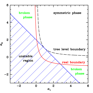
Figure 2.2: The schematic phase diagram in the $\alpha_{1}-\alpha_{2}$ plane. The dashed line represents the tree level phase boundary, while the solid line shows the real boundary. The shaded region is unstable where the action is not bounded from below.

Figure 2.2 shows the schematic phase diagram of MSSM in the $\alpha_{1}-\alpha_{2}$ plane. We can observe the renormalization effects on the phase boundary. The tree level boundary is $\alpha_{1}\cdot\alpha_{2}=1$ while the real boundary (determined from a few simulation points) has a similar shape but it is shifted. It is interesting that the phase boundary is more shifted in the $\alpha_{2}$ direction than in the $\alpha_{1}$ direction. This is caused by the large top Yukawa coupling since it gives a dominant renormalization contribution to $\alpha_{2}$ only.

Simulations were performed in two main steps:

1. Finite temperature simulations, when the temporal extension $L_{t}$ of the lattice is much smaller than the spatial extensions $L_{x,y,z}$. For a given $L_{t}$ we fixed all parameters of the Lagrangian except $\alpha_{2}$. We used $\alpha_{2}$ to tune the system to the transition point. For finding the transition point, two different methods were used which I will discuss in more details later. We measured the jump of the expectation value of the Higgs fields in the transition point. Using lattices with different spatial extensions, we performed infinite volume extrapolations both for the critical $\alpha_{2}$ and the Higgs jump.

2. Zero temperature simulations. We used large lattices (with large $L_{t}$ as well). $\alpha_{2}$ was set to its infinite volume extrapolated value, while all other parameters were set to be the same as in the finite temperature case. We measured the correlation functions for the $W$ and Higgs bosons and Wilson-loops. The $W$ correlation length gives the inverse $W$ mass in lattice units which determines the lattice spacing. This makes it possible to express our quantities in physical units rather than in lattice units.

Both steps were performed for different lattice spacings. The lattice spacing can be changed by changing the temporal extension of the finite temperature lattice. We used four different temporal extensions, $L_{t}=2,3,4,5$. While changing the lattice spacing, we have to change the bare parameters of the Lagrangian so that all zero temperature observables remain the same. We want to keep the system on a line of constant physics (LCP).

2.4.1 Finite temperature simulations

The first goal of finite temperature simulations is to determine the critical value of $\alpha_{2}$ at which a first order phase transition occurs. Depending on the strength of the phase transition, different methods can be efficiently used to find the value of $\alpha_{2c}$ accurately. First one can get a rough estimate on $\alpha_{2c}$ if simulations are performed for several different $\alpha_{2}$ values. A change can be observed in the length of the second Higgs field $|H_{2}|^{2}$ around the critical point. Then collecting large statistics near the critical point, the Ferrenberg-Swendsen reweighting technique [19] can be applied to get information about observables belonging to slightly different $\alpha_{2}$ values. We used two different methods to find the critical point.

Lee-Yang zeros

The method of Lee-Yang zeros [20] can be applied if the phase transition is not too strong and during the simulations the system can walk between the different phases.

The free energy is singular in a first order phase transition point, which means that the partition function vanishes. For finite volumes the free energy singularity, the roots of the partition function will not be real any more. If we analytically continue the partition function into the complex $\alpha_{2}$ plane, we can find these zeroes. Fortunately as we increase the lattice volume, the imaginary parts of these Lee-Yang zeros tend to be zero. The partition function at arbitrary $\alpha_{2}$ (not too far from the simulation point) can be obtained by the reweighting mentioned before. We may then look for the zeros of the partition function in the complex plane and the real part of the root with smallest imaginary part will give the critical point to a high accuracy.

Constrained simulations

Lee-Yang zeros can not be found (or fake zeros are found) if the phase transition is too strong. In these cases the system is usually stuck into one of the phases and due to the ”supercritical slowing down” the updating algorithm is not able to evolve it to the other phase.

A solution to this problem is not to let the system go to any of the phases. Instead, we constrain the value of the order parameter (in our case $|H_{2}|^{2}$ averaged over the lattice) in a small interval between the two phases [21]. All configurations that have an order parameter out of this interval are rejected. If we are at the critical point then the system can minimize its free energy in a way that two separate phases are formed at two different parts of the lattice. The definition of the critical point is in this case that the distribution of the order parameter on the selected interval should be uniform. This definition may slightly depend on the choice of the interval between the two phases, however, this dependence vanishes in the infinite volume limit.

Finite temperature results

In the following I present the results of finite temperature simulations. Four different temporal lattice extensions were used ($L_{t}=2,3,4,5$). Figure 2.3 shows the distribution of the order parameter in the transition point on a $4^{3}\times 2$ lattice. It is easy to identify the two phases, the transition is clearly of first order.

Figure 2.3: The distribution of the order parameter $|H_{2}|^{2}$ in the transition point. The two separate peaks clearly indicate a first order phase transition.

Using the method of Lee-Yang zeros, the critical $\alpha_{2}$ value was found for several spatial lattice extensions. Figure 2.4 shows the finite volume scaling of critical points for $L_{t}=3$. One can observe that the critical points scale well with $1/V$ (except for the smallest volumes) and this property can be used to extrapolate to infinite volume. The infinite volume $\alpha_{2}$ is found to be $\alpha_{2c}=-0.96137(3)$. The jump of the order parameter can be measured from histograms like Figure 2.3 and an infinite volume extrapolation can also be done.

Figure 2.4: The critical $\alpha_{2}$ values for different lattice volumes as a function of the inverse volume.

Table 2.1 shows $\alpha_{2c}$ and $v/T$ for the four different temporal extensions. The errors were obtained by using a jackknife analysis. We can observe that both $\alpha_{2c}$ and the Higgs jump increases as we go to the continuum limit.

$L_{t}$	$2$	$3$	$4$	$5$
$\alpha_{2c}$	-1.0005(5)	-0.96137(3)	-0.9575(1)	-0.95504(2)
$v/T$	1.50(1)	1.83(5)	1.99(2)	2.12(1)

Table 2.1: The critical $\alpha_{2}$ values and $v/T$ for different temporal lattice extensions.

2.4.2 Zero temperature simulations

After performing finite temperature simulations and finding the critical $\alpha_{2}$ values we have to carry out zero temperature simulations to measure the mass spectrum at the given physical point. The masses of particles can be extracted from two-point functions of field operators. For the Higgs mass we measured the correlation functions:

$$c_{ij}(x,y)=<|H_{i}(x)|^{2}|H_{j}(y)|^{2}>,$$ (2.18)

with $i,j=1,2$ for the two Higgs fields. The lightest Higgs mass can be obtained from the exponential tails of these correlation functions. For the $W$ mass the same operators were used as in [8]. The results for the Higgs and $W$ masses and their ratio $R_{HW}$ is given in Table 2.2. The errors were calculated again by a jackknife analysis. We can see from the data that not an exact line of constant physics was followed. Thus we need perturbative corrections which we include in the next section.

$L_{t}$	$2$	$3$	$4$	$5$
$m_{H}$	0.325(6)	0.124(10)	0.088(6)	0.070(10)
$m_{W}$	0.594(12)	0.335(8)	0.253(18)	0.211(20)
$R_{HW}$	0.547(15)	0.370(31)	0.348(34)	0.332(57)

Table 2.2: The lightest Higgs and $W$ masses in lattice units and their ratio for different temporal lattice extensions. $L_{t}$ is the temporal lattice extension of the corresponding finite temperature lattice.

2.5 Comparison with perturbation theory

We compared our simulation results with perturbation theory. We used one-loop perturbation theory without applying high temperature expansion (HTE). A specific feature was a careful treatment of finite renormalization effects, by taking into account all renormalization corrections and adjusting them to match the measured zero temperature spectrum [22]. We studied also the effect of the dominant finite temperature two-loop diagram (“setting-sun” stop-gluon graphs, cf. fifth ref. of [12]), but only in the HTE. Since the infrared behavior of the setting-sun graphs is not fully understood, we used the one-loop technique with the zero temperature scheme defined above. This type of one-loop perturbation theory was also applied to correct the measured data to some fixed LCP quantities, which are defined as the averages of results at different lattice spacings, (i.e. our reference point, for which the most important quantity is the lightest Higgs mass).

The bare squark mass parameters $m_{Q}^{2},m_{U}^{2},m_{D}^{2}$ receive quadratic renormalization corrections. As it is well-known, one-loop lattice perturbation theory is not sufficient to determine these corrections reliably, thus we used the following method. We first determined the position of the non-perturbative color-breaking phase transitions in the bare quantities (see next section). These quantities were compared with the prediction of the continuum perturbation theory, which yielded the renormalized mass parameters on the lattice.

Figure 2.5 contains the continuum limit extrapolation for the normalized jump of the order parameter ($v/T_{c}$: upper data) and the critical temperature ($T_{c}/m_{W}$: lower data). The shaded regions are the perturbative predictions at our reference point (see above) in the continuum. Their widths reflect the uncertainty of our reference point, which is dominated by the error of $m_{h}$. Note that $v/T_{c}$ is very sensitive to $m_{h}$, which results in the large uncertainties. Results obtained on the lattice and in perturbation theory agree reasonably within the estimated uncertainties. It might well be that the $L_{t}$=2 results are not in the scaling region; leaving them out from the continuum extrapolation the agreement between the lattice and perturbative results is even better.

Figure 2.5: The normalized jump and the critical temperature in the continuum limit.

2.6 The phase diagram of bosonic MSSM

As the bare squark mass parameter $m_{U}^{2}$ is decreased, the system can go to a so-called color-breaking phase where the SU(3) symmetry is spontaneously broken. As mentioned in the previous section, the knowledge of this well-defined transition point helps us to perform the squark mass renormalization. We determined the phase diagram in the $m_{U}^{2}$–$\alpha_{2}$ plane in the infinite volume limit and after performing zero temperature simulations we could transform it to the physical $m_{U}^{2}$–$T$ scales. The phase transition to the color-breaking phase is much stronger than the one between the symmetric and Higgs phases, so we used the constrained simulation method to obtain the critical $m_{U}^{2}$ values.

Figure 2.6. shows the phase diagram in the $m_{U}^{2}$–T plane. One can identify three phases. The phase on the left (large negative $m_{U}^{2}$ and small stop mass) is the color-breaking phase. The phase in the upper right part is the symmetric phase, whereas the Higgs phase can be found in the lower right part. The line separating the symmetric and Higgs phases was obtained from the $L_{t}=3$ simulations, whereas the lines between these phases and the color-breaking one were determined by keeping the lattice spacing fixed, while increasing and decreasing the temperature by changing $L_{t}$ to 2 and 4, respectively. The shaded regions indicate the uncertainty in the critical temperatures. The qualitative features of this picture are in complete agreement with perturbative and 3d lattice results [12, 13, 14]; however, our choice of parameters does not correspond to a two-stage symmetric-Higgs phase transition. In this two-stage scenario there is a phase transition from the symmetric to the color-breaking phase at some $T_{1}$ and another phase transition occurs at $T_{2}<T_{1}$ from the color-breaking to the Higgs phase. It has been argued [23] that in the early universe no two-stage phase transition took place.

Figure 2.6: The phase diagram of the bosonic theory obtained by lattice simulations.

2.7 Analysis of the bubble wall

In order to produce the observed baryon asymmetry, a strong first order phase transition is not enough. According to standard MSSM baryogenesis scenarios [18] the generated baryon asymmetry is directly proportional to the variation of $\beta$ through the bubble wall separating the Higgs and symmetric phases. By using elongated lattices ($2\cdot L^{2}\cdot 192$), $L$=8,12,16 at the transition point we studied the properties of the wall. We performed constrained simulations in the transition point (see section 2.4.1). The length of the second Higgs field was restricted to a small interval between its values in the bulk phases. As a consequence, the system fluctuated around a configuration with two bulk phases and two walls between them. In order to have the smallest possible free energy, the walls are perpendicular to the long direction. To find the wall profile we measured the average of both Higgs fields on each timeslice separately. When taking the averages of the wall profiles one has to be careful. Due to translational symmetry the location of the walls is different for different configurations. Before taking an average the different configurations should be appropriately shifted. The required shift between two samples can be obtained by minimizing the following ”distance”:

$$d=\sum_{i=1}^{192}{\frac{\left(\Phi_{1i}-\Phi_{2(i+k)}\right)^{2}}{\sigma_{1i}^{2}+\sigma_{2(i+k)}^{2}}},$$ (2.19)

where $\Phi_{1i}$ ($\Phi_{2(i+k)}$) is the average of one of the Higgs fields on the $i$-th ($i+k$-th) timeslice on the first (second) sample and the $\sigma$-s are the corresponding standard deviations. $k$ is the relative shift of the two samples ($i+k$ is of course meant by modulo 192).

Figure 2.7 shows the bubble wall profiles for both Higgs fields after averaging ${\cal O}(50000)$ configurations for $L=12$. The wall profiles are similar for $L=8$ and $L=16$. The width of the wall ($w$) can be obtained by fitting $a+b\cdot\tanh(\frac{2(x-x_{0})}{w})$ to the wall profile. The width slightly depends on the cross size of the lattice. We found $w=[A+B\cdot\log(aLT_{c})]/T_{c}$ with $A=10.8\pm.1$ and $B=2.1\pm.1$. This behavior indicates that the bubble wall is rough and without a pining force of finite size its width diverges very slowly (logarithmically) [24]. For the same bosonic theory the perturbative approach predicts $(11.2\pm 1.5)/T_{c}$ for the width.

Figure 2.7: The profile of the bubble wall for both of the Higgs fields for the lattice $2\cdot 12^{2}\cdot 192$.

Figure 2.8: The relation between the Higgs fields within the bubble wall. The variation of $beta$ through the wall can be determined by de slopes at the two ends.

Transforming the data of Figure 2.7 to $|H_{2}|^{2}$ as a function of $|H_{1}|^{2}$, we obtain Figure 2.8. We can see that the relation between the lengths of the Higgs fields is almost linear. However, the slopes at the two ends significantly differ. From this difference we can compute the variation of $\beta$ through the bubble wall: $\Delta\beta=0.0061\pm 0.0003$. The perturbative prediction at this point is $0.0046\pm 0.0010$. Thus perturbative studies such as [25] are confirmed by non-perturbative results.

The errors of the wall width and $\Delta\beta$ were found by a jackknife analysis.

Chapter 3 Ultrahigh energy cosmic rays

The existence of Ultrahigh energy cosmic rays (UHECRs) – those with energy above $10^{20}$ eV – is a real challenge for conventional theories of their origin based on acceleration of charged particles.

The current theories of UHECR can be divided into two broad classes: the ”bottom-up” and ”top-down” scenarios. They are opposite to each other. In the ”bottom-up” scenarios it is assumed that UHECRs are accelerated from lower enegries in special astrophysical environments. Some examples are acceleration in shocks associated with supernova remnants, active galactic nuclei (AGNs), powerful radio galaxies, or acceleration in the strong electric fields generated by rotating neutron stars. In the ”top-down” scenarios UHECRs are the decay products of some yet unknown metastable superheavy particles.

If these UHECRs are conventional particles such as nuclei or protons, then above energies of $4\times 10^{19}$ eV they loose a large fraction of their energy due to the Greisen-Zatsepin-Kuzmin (GZK) effect [26]. This predicts a sharp drop in the cosmic ray flux above the GZK cutoff around $4\cdot 10^{19}$ eV. The available data shows no such drop. About 20 events above $10^{20}$ eV were observed by a number of experiments such as AGASA [27], Fly’s Eye [28], Haverah Park [29], Yakutsk [30] and HiRes [31]. Since above the GZK energy the attenuation length of particles is a few tens of megaparsecs [32, 33, 34, 35], if an UHECR is observed on earth it must be produced in our vicinity (except for UHECR scenarios based on weakly interacting particles, e.g. neutrinos [36]).

Usually it is assumed that at these high energies the galactic and extragalactic magnetic fields do not affect the orbit of the cosmic rays, thus they should point back to their origin within a few degrees. In contrast to the low energy cosmic rays one can use UHECRs for point-source search astronomy. (For an extragalactic magnetic field of $\mu$G rather than the usually assumed nG there is no directional correlation with the source [37].)

Though there are some peculiar clustered events [38, 39], which we discuss in detail in the next section [40], the overall distribution of UHECR on the sky is practically isotropic [41]. This observation is rather surprising since in principle only a few astrophysical sites (e.g. active galactic nuclei [42] or the extended lobes of radio galaxies [43]) are capable of accelerating such particles. Nevertheless none of the UHECR events came from these directions [44]. Sources of extragalactic origin (e.g. AGN [45], topological defects [46] or the local supercluster [47]) should result in a GZK cutoff, which is in disagreement with experiments. Hence it is generally believed [48] that there is no conventional astrophysical explanation for the observed UHECR spectrum.

The ”top-down” scenarios are other candidates to explain the highest energy events. This possibility will be discussed in section 3.2. I will concentrate on the determination of the mass scale of the superheavy $X$ particle. The existence of these $X$ particles would clearly point beyond the Standard Model and the most interesting result is that the $m_{X}$ obtained using the experimental data is consistent with the GUT scale [49].

3.1 Clustering of UHECR events

The arrival directions of the UHECRs measured by experiments show some peculiar clustering: some events are grouped within $\sim 3^{o}$, the typical angular resolution of an experiment. Above $4\cdot 10^{19}$ eV 92 cosmic ray events were detected, including 7 doublets and 2 triplets. Above $10^{20}$ eV one doublet out of 14 events was found [39]. The chance probability of such a clustering from uniform distribution is rather small [39, 38]. (Taking the average bin $3^{o}$ the probability of generating one doublet out of 14 events is $11\%$.)

The clustered features of the events initiated an interesting statistical analysis assuming compact UHECR sources [50]. The authors found a large number, $\sim 400$ for the number of sources inside a GZK sphere of 25 Mpc. They assumed that a.) the number of clustered events is much smaller than the total number of events (this is a reliable assumption at present statistics; however, for any number of sources the increase of statistics, which will happen in the near future, results in more clustered events than unclustered); b.) all sources have the same luminosity which gives a delta function for their distribution (this unphysical choice represents an important limit, it gives the smallest source density for a given number of clustered and unclustered events). c.) The GZK effect makes distant sources fainter; however, this feature depends on the injected energy spectrum and the attenuation lengths and elasticities of the propagating particles. In [50] an exponential decay was used with an energy independent decay length of 25Mpc.

In our approach none of these assumptions were used. In addition we included spherical astronomy corrections and in particular determined the upper and lower bounds for the source density at a given confidence level. As it will be shown, the most probable value for the source density is really large; however, the statistical significance of this result is rather small. At present the small number of UHECR events allows a 95% confidence interval for the source density which spreads over four orders of magnitude. Since future experiments, particularly Pierre Auger [51], will have a much higher statistical significance on clustering (the expected number of events of $10^{20}$ eV and above is 60 per year [52]), we present our results on the density of sources also for larger number of UHECRs above $10^{20}$ eV.

In order to avoid the assumptions of [50] a combined analytical and Monte-Carlo technique will be presented adopting the conventional picture of protons as the ultrahigh energy cosmic rays. Our analytical approach of Section 3.1.1 gives the event clustering probabilities for any space, luminosity and energy distribution of the sources by using a single additional function $P(r,E;E_{c})$, the probability that a proton created at a distance $r$ with energy $E$ arrives at earth above the threshold energy $E_{c}$ [53]. With our Monte-Carlo technique of Section 3.1.2 we determine the probability function $P(r,E,E_{c})$ for a wide range of parameters.

3.1.1 Analytical approach

The key quantity for finding the distribution functions for the source density, is the probability of detecting $k$ events from one randomly placed source. The number of UHECRs emitted by a source of $\lambda$ luminosity during a period $T$ follows the Poisson distribution. However, not all emitted UHECRs will be detected. They might loose their energy during propagation or can simply go to the wrong direction.

For UHECRs the energy loss is dominated by the pion production in interaction with the cosmic microwave background radiation. In ref. [53] the probability function $P(r,E,E_{c})$ was presented for three specific threshold energies. This function gives the probability that a proton created at a given distance from earth (r) with some energy (E) is detected at earth above some energy threshold ($E_{c}$). The resulting probability distribution can be approximated over the energy range of interest by a function of the form

$$P(r,E,E_{c})\approx\exp[-a(E_{c})r^{2}\exp(b(E_{c})/E)]$$ (3.1)

The appropriate values of $a$ and $b$ for $E_{c}/(10^{20}{\rm eV})=$1,3, and 6 are, respectively $a/(10^{-4}{\rm Mpc}^{-2})=$1.4, 9.2 and 11, $b/(10^{20}eV)=$2.4, 12 and 28.

For the sources we use the second equatorial coordinate system: ${\bf x}$ is the position vector of the source characterized by ($r,\delta,\alpha$) with $\delta$ and $\alpha$ being the declination and right ascension, respectively. The features of the Poisson distribution enforce us to take into account the fact that the sky is not isotropically observed. There is a circumpolar cone, in which the sources can always be seen, with half opening angle $\delta^{\prime}$ ($\delta^{\prime}$ is the declination of the detector, for the experiments we study $\delta^{\prime}\approx 40^{o}-50^{o}$). There is also an invisible region with the same opening angle. Between them there is a region for which the time fraction of visibility, $\gamma(\delta,\delta^{\prime})$ is a function of the declination of the source. It is straightforward to determine $\gamma(\delta,\delta^{\prime})$ for any $\delta$ and $\delta^{\prime}$:

$$\gamma(\delta,\delta^{\prime})=\left\{\begin{array}[]{lll}0&\mbox{if }&-\pi/2<\delta\leq\delta^{\prime}-\pi/2\\ 1-&\arccos&(\tan\delta^{\prime}\tan\delta)/\pi\\ &\mbox{if }&\delta^{\prime}-\pi/2<\delta\leq\pi/2-\delta^{\prime}\\ 1&\mbox{if }&\pi/2-\delta^{\prime}<\delta\leq\pi/2\end{array}\right.$$ (3.2)

To determine the probability that a particle arriving from random direction at a random time is detected we have to multiply $\gamma(\delta,\delta^{\prime})$ by the cosine of the zenith angle $\theta$. In the following we will use the time average of this function:

$$\eta(\delta,\delta^{\prime})=\frac{1}{T}\int_{0}^{T}{\gamma(\delta,\delta^{\prime})\cdot\cos\theta(\delta,\delta^{\prime},t)dt}$$ (3.3)

Since $\delta^{\prime}$ is constant, in the rest of the paper we do not indicate the dependence on it. Neglecting these spherical astronomy effects means more than a factor of two for the prediction of the source density.

The probability of detecting $k$ events from a source at distance $r$ with energy $E$ can be obtained by including $P(r,E,E_{c})A\eta(\delta)/(4\pi r^{2})$ in the Poisson distribution:

$$p_{k}({\bf x},E,j)=\frac{\exp\left[-P(r,E,E_{c})\eta(\delta)j/r^{2}\right]}{k!}\times$$

$$\left[P(r,E,E_{c})\eta(\delta)j/r^{2}\right]^{k},$$ (3.4)

where we introduced $j=\lambda TA/(4\pi)$ and $A\eta(\delta)/(4\pi r^{2})$ is the probability that an emitted UHECR points to a detector of area $A$. We denote the space, energy and luminosity distributions of the sources by $\rho({\bf x})$, $c(E)$ and $h(j)$, respectively. The probability of detecting $k$ events above the threshold $E_{c}$ from a single source randomly positioned within a sphere of radius $R$ is

$$P_{k}=\int_{S_{R}}dV\;\rho({\bf x})\int_{E_{c}}^{\infty}dE\;c(E)\int_{0}^{\infty}dj\;h(j)\times$$

$$\frac{\exp\left[-P(r,E,E_{c})\eta(\delta)j/r^{2}\right]}{k!}\left[P(r,E,E_{c})\eta(\delta)j/r^{2}\right]^{k}.$$ (3.5)

Denote the total number of sources within the sphere of sufficiently large radius (e.g. several times the GZK radius) by $N$ and the number of sources that gave $k$ detected events by $N_{k}$. Clearly, $N=\sum_{0}^{\infty}N_{i}$ and the total number of detected events is $N_{e}=\sum_{0}^{\infty}iN_{i}$. The probability that for $N$ sources the numbers of different detected multiplets are $N_{k}$ is:

$$P(N,\{N_{k}\})=N!\prod_{k=0}^{\infty}\frac{1}{N_{k}!}P_{k}^{N_{k}}.$$ (3.6)

The value of $P(N,\{N_{k}\})$ is the most important quantity in our analysis of UHECR clustering. For a given set of unclustered and clustered events ($N_{1}$ and $N_{2},N_{3}$,…) inverting the $P(N,\{N_{k}\})$ distribution function gives the most probable value for the number of sources and also the confidence interval for it. If we want to determine the density of sources we can take the limit $R\rightarrow\infty,N\rightarrow\infty$, while the density of sources $S=N/(\frac{4}{3}R^{3}\pi)$ is constant.

In order to illustrate the dominant length scale it is instructive to study the integrand $f_{k}(r)$ of the distance integration in eqn. (3.1.1)

$$P_{k}=\int_{0}^{R}\left(\frac{dr}{R}\right)f_{k}(r),$$

$$f_{k}(r)=Rr^{2}\int d\Omega\rho({\bf x})\int_{E_{c}}^{\infty}dE\;c(E)\int_{0}^{\infty}dj\;h(j)\times$$

$$\frac{\exp\left[-P(r,E,E_{c})\eta(\delta)j/r^{2}\right]}{k!}\left[P(r,E,E_{c})\eta(\delta)j/r^{2}\right]^{k}.$$ (3.7)

Figure 3.1 shows that $f_{1}(r)$, which leads to singlet events, is dominated by the distance scale of 10-15 Mpc, whereas $f_{2}(r)$, which gives doublet events, is dominated by the distance scale of 4-6 Mpc. It is interesting that the dominant distance scale for singlet events is by an order of magnitude smaller than the attenuation length of the protons at these energies ($l_{a}\approx 110$ Mpc). This surprising result can be illustrated using a simple approximation. Assuming that the probability of detecting a particle coming from distance $r$ is proportional to $exp(-r/l_{a})/r^{2}$, $P_{1}$ will be proportional to $\int d\Omega drr^{2}\cdot\exp[-j\exp(-r/l_{a})/r^{2}]\cdot\exp(-r/l_{a})/r^{2}$. For the typical $j$ values the $r$ integrand has a maximum around 4 Mpc and not at $l_{a}$. These typical distances partly justify our assumption of neglecting magnetic fields. The deflection of singlet events due to magnetic fields does not change the number of multiplets, thus our conclusions remain unchanged. The typical distance for higher multiplets is quite small, therefore deflection can be practically neglected. Clearly, the fact that multiplets are coming from our “close” neighborhood does not mean that the experiments reflect just the densities of these distances. The overwhelming number of events are singlets and they come from much larger distances. Note, that these $f_{1}(r)$ and $f_{2}(r)$ functions were obtained with our optimal $j_{*}$ value (cf. Figure 3.5 and explanation there and in the corresponding text). Using the largest possible $j_{*}$ value allowed by the 95% confidence region the dominant distance scales for $f_{1}(r)$ and $f_{2}(r)$ functions turn out to be 30 Mpc and 20 Mpc, respectively.

Figure 3.1: The distributions $f_{1}(r)$ –solid line– and $f_{2}(r)$ –dashed line– of eqn. (3.1.1). The singlet and doublet events are dominated by distance scale of 10-15 Mpc and 3-5 Mpc, respectively.

Note, that $P_{k}$ and then $P(N,\{N_{k}\})$ are easily determined by a well-behaved four-dimensional numerical integration (the $\alpha$ integral can be factorized) for any $c(E)$, $h(j)$ and $\rho(r)$ distribution functions . In order to illustrate the uncertainties and sensitivities of the results we used a few different choices for these distribution functions.

For $c(E)$ we studied three possibilities. The most straightforward choice is the extrapolation of the ‘conventional high energy component’ $\propto E^{-2}$. Another possibility is to use a stronger fall-off of the spectrum at energies just below the GZK cutoff, e.g. $\propto E^{-3}$. These choices span the range usually considered in the literature and we will study both of them. The third possibility is to assume that topological defects generate UHECRs through production of superheavy particles . According to [56] these superheavy particles decay into quarks and gluons which initiate multi-hadron cascades through gluon bremsstrahlung. These finally hadronize to yield jets. The energy spectrum was first calculated in [59] for the Standard Model and in [60] for the Minimal Supersymmetric Standard Model. In Section 3.2 we will determine the decay spectrum of $X$ particles and find the $m_{X}$ for which the agreement with observations is the best. We used this spectrum as the third choice of energy distribution, $c(E)$.

In ref. [50] the authors have shown that for a fixed set of multiplets the minimal density of sources can be obtained by assuming a delta-function distribution for $h(j)$. We studied both this limiting case ($h(j)=\delta(j-j_{*})$) and a more realistic one with Schechter’s luminosity function [61]:

$$h(j)dj=h\cdot(j/j_{*})^{-1.25}\exp(-j/j_{*})d(j/j_{*}).$$ (3.8)

The space distribution of sources can be given based on some particular survey of the distribution of nearby galaxies [62] or on a correlation length $r_{0}$ characterizing the clustering features of sources [53]. For simplicity the present analysis deals with a homogeneous distribution of sources randomly scattered in the universe (Note, that due to the Local Supercluster the isotropic distribution is just an approximation.).

Figure 3.2: The individual $P_{k}(j_{*})$ functions for the different $c(E)$ and $h(j)$ choices. The column on the left corresponds to the Dirac-delta distribution $h(j)=\delta(j-j_{*})$, whereas the column on the right shows the results for Schechter’s luminosity distribution. The first, second and third rows correspond to the $c(E)$ functions proportional to $E^{-2}$, $E^{-3}$ and the superheavy decay mode, respectively (see text). On each panel the individual lines from top to bottom are: $1-P_{0}$, $P_{1}$, $P_{2}$, $P_{3}$, $P_{4}$ and $P_{5}$.

Figure 3.2 shows the resulting $P_{k}(j_{*})$ probability functions for the different choices of $c(E)$ and $h(j)$. The overall shapes of them are rather similar; nevertheless, relatively small differences lead to quite different predictions for the UHECR source density. The “shoulders” of the curves with Dirac-delta luminosity distributions got smoother for Schechter’s distribution. The scales on the figures are chosen to cover the 95% confidence regions (see section 3.1.3 for details).

Note, that – assuming that UHECRs point back to their sources – our clustering technique discussed above applies to practically any models of UHECR (e.g. neutrinos). One only needs a change in the $P(r,E,E_{c})$ probability distribution function (e.g. neutrinos penetrate the microwave background uninhibited) and use the $h(j)$ and $c(E)$ distribution function of the specific model.

3.1.2 Monte-Carlo study of the propagation

Our Monte-Carlo model of UHECR studies the propagation of UHECR. The analysis of [63] showed that both AGASA and Fly’s Eye data demonstrated a change of composition, a shift from heavy –iron– at $10^{17}$ eV to light –proton– at $10^{19}$ eV. Thus, the chemical composition of UHECRs is most likely to be dominated by protons. In our analysis we use exclusively protons as UHECR particles. (For suggestions that air showers above the GZK cutoff are induced by neutrinos see [36].)

Using the pion production as the dominant effect of energy loss for protons at energies $>10^{19}$ eV ref. [53] calculated $P(r,E,E_{c})$, the probability that a proton created at a given distance (r) with some energy (E) is detected at earth above some energy threshold ($E_{c}$). For three threshold energies the authors of [53] gave the approximate formula (3.1).

In our Monte-Carlo approach we determined the propagation of UHECR on an event by event basis. Since the inelasticity of Bethe-Heitler pair production is rather small ($\approx 10^{-3}$) we used a continuous energy loss approximation for this process. The inelasticity of pion-photoproduction is much higher ($\approx 0.2-0.5$) in the energy range of interest, thus there are only a few tens of such interactions during the propagation. Due to the Poisson statistics of the number of interactions and the spread of the inelasticity, we will see a spread in the energy spectrum even if the injected spectrum is mono-energetic.

In our simulation protons propagate in small steps ($10$ kpc), and after each step the energy losses due to pair production, pion production and the adiabatic expansion are calculated. During the simulation we keep track of the current energy of the proton and its total displacement. Thus, one avoids performing new simulations for different initial energies and distances. The propagation is completed when the energy of the proton goes below a given cutoff ($10^{18}$ eV in our case). For the proton interaction lengths and inelasticities we used the values of [33, 34]. The deflection due to magnetic fields is not taken into account, because it is small for our typical distances illustrated in Figure 3.1. This fact justifies our assumption that UHECRs point back to their sources (for a recent Monte-Carlo analysis on deflection see e.g. [35]).

Figure 3.3: The direct Monte-Carlo points and the fitted function $P(r,E,E_{c})=\exp\left[-a\cdot(r/\ {\rm 1Mpc})^{b}\right]$ for $E_{c}=10^{20}$ eV and $E=2\cdot 10^{20}$ eV. The fitted curve corresponds to $a=0.0019$ and $b=1.695$.

Since it is rather practical to use the $P(r,E,E_{c})$ probability distribution function we extended the results of [53] by using our Monte-Carlo technique for UHECR propagation. In order to cover a much broader energy range than the parametrization of (3.1) we used the following type of function

$$P(r,E,E_{c})=\exp\left[-a\cdot(r/1\ {\rm Mpc})^{b}\right].$$ (3.9)

Figure 3.3 demonstrates the reliability of this parametrization. The direct Monte-Carlo points and the fitted function (eqn. (3.9) with $a=0.0019$ and $b=1.695$) are plotted for $E_{c}=10^{20}$eV and $E=2\cdot 10^{20}$eV.

Figure 3.4: The functions $a(E/E_{c})$ –left panel– and $b(E/E_{c})$ –right panel– for the probability distribution function $P(r,E,E_{c})$ using the parametrization $\exp[-a\cdot(r/1\ {\rm Mpc})^{b}]$ for five different threshold energies ($5\cdot 10^{19}$ eV, $10^{20}$ eV, $2\cdot 10^{20}$ eV, $5\cdot 10^{20}$ eV and $10^{21}$ eV).

Figure 3.4 shows the functions $a(E/E_{c})$ and $b(E/E_{c})$ for a range of three orders of magnitude and for five different threshold energies. Just using the functions of $a(E/E_{c})$ and $b(E/E_{c})$, thus a parametrization of $P(r,E,E_{c})$ one can obtain the observed energy spectrum for any injection spectrum without additional Monte-Carlo simulation.

3.1.3 Density of sources

In order to determine the confidence intervals for the source densities we used the frequentist method[64]. We wish to set limits on S, the source density. Using our Monte-Carlo based $P(r,E,E_{c})$ functions and our analytical technique we determined $p(N_{1},N_{2},N_{3},...;S;j_{*})$, which gives the probability of observing $N_{1}$ singlet, $N_{2}$ doublet, $N_{3}$ triplet etc. events if the true value of the density is $S$ and the central value of luminosity is $j_{*}$. The probability distribution is not symmetric and far from being Gaussian. For a given set of $\{N_{i},i=1,2,...\}$ the above probability distribution as a function of $S$ and $j_{*}$ determines the 68% and 95% confidence level regions in the $S-j_{*}$ plane. Figure 3.5 shows these regions for our “favorite” choice of model ($c(E)\propto E^{-3}$ and Schechter’s luminosity distribution) and for the present statistics (one doublet out of 14 UHECR events). The regions are deformed, thin ellipse-like objects in the $\log(j_{*})$ versus $\log(S)$ plane. Since $j_{*}$ is a completely unknown and independent physical quantity the source density can be anything between the upper and lower parts of the confidence level regions. For this model our final answer for the density is $180_{-165(174)}^{+2730(8817)}\cdot 10^{-3}$ Mpc^-3, where the first errors indicate the 68%, the second ones in the parenthesis the 95% confidence levels, respectively. The choice of [50] –Dirac-delta like luminosity distribution– and, for instance, conventional $E^{-2}$ energy distribution gives much smaller value: $2.77_{-2.53(2.70)}^{+96.1(916)}10^{-3}$ Mpc^-3. For other choices of $c(E)$ and $h(j)$ see Table 3.1. Our results for the Dirac-delta luminosity distribution are in agreement with the result of [50] within the error bars. Nevertheless, there is a very important message. The confidence level intervals are so large, that on the 95% confidence level two orders of magnitude smaller densities than suggested as a lower bound by [50] are also possible.

Figure 3.5: The $1\sigma$ (68%) and $2\sigma$ (95%) confidence level regions for $j_{*}$ and the source density (14 UHECR with one doublet). The most probable value is represented by the triangle. The upper and lower boundaries of these regions give for the source density $180_{-165(174)}^{+2730(8817)}\cdot 10^{-3}$ Mpc^-3 on the 68% (95%)confidence level.

As it can be seen there is a strong correlation between the luminosity and the source density. Physically it is easy to understand the picture. For a smaller source density the luminosities should be larger to give the same number of events. However, it is not possible to produce the same multiplicity structure with arbitrary luminosities. Very small luminosities can not give multiplets at all, very large luminosities tend to give more than one doublet.

$c(E)$	$h(j)$	14 events 1 doublet
$\propto E^{-2}$	$\propto\delta$	$2.77_{-2.53(2.70)}^{+96.1(916)}$
$\propto E^{-2}$	$\propto$ SLF	$36.6_{-34.3(35.9)}^{+844(4268)}$
$\propto E^{-3}$	$\propto\delta$	$5.37_{-4.98(5.25)}^{+80.2(624)}$
$\propto E^{-3}$	$\propto$ SLF	$180_{-165(174)}^{+2730(8817)}$
$\propto$ decay	$\propto\delta$	$3.61_{-3.30(3.51)}^{+116(1060)}$
$\propto$ decay	$\propto$ SLF	$40.9_{-38.3(40.1)}^{+856(4345)}$
$c(E)$	$h(j)$	24 events 1 doublet
$\propto E^{-2}$	$\propto\delta$	$17.4_{-16.0(17.0)}^{+298(2790)}$
$\propto E^{-2}$	$\propto$ SLF	$200_{-169(182)}^{+1230(2428)}$
$\propto E^{-3}$	$\propto\delta$	$25.0_{-22.6(24.3)}^{+211(1690)}$
$\propto E^{-3}$	$\propto$ SLF	$965_{-741(821)}^{+3220(5613)}$
$\propto$ decay	$\propto\delta$	$20.4_{-18.6(19.9)}^{+358(3190)}$
$\propto$ decay	$\propto$ SLF	$211_{-174(190)}^{+1110(2274)}$
$c(E)$	$h(j)$	24 events 2 doublets
$\propto E^{-2}$	$\propto\delta$	$3.19_{-2.68(2.99)}^{+26.4(253)}$
$\propto E^{-2}$	$\propto$ SLF	$41.5_{-36.4(40)}^{+424(1514)}$
$\propto E^{-3}$	$\propto\delta$	$6.42_{-5.46(6.07)}^{+46.2(193)}$
$\propto E^{-3}$	$\propto$ SLF	$208_{-182(201)}^{+1970(3858)}$
$\propto$ decay	$\propto\delta$	$4.18_{-3.51(3.92)}^{+34.5(296)}$
$\propto$ decay	$\propto$ SLF	$45.4_{-39.7(43.7)}^{+457(1556)}$

Table 3.1: The most probable values for the source densities and their error bars given by the 68% and 95% confidence level regions (the latter in parenthesis). The numbers are in units of $10^{-3}$ Mpc^-3 The three possible energy spectrums are given by a distribution proportional to $E^{-2}$, $E^{-3}$, or by the decay of a $10^{12}$ GeV particle (denoted by “decay”). The luminosity distribution can be proportional to a Dirac-delta or to Schechter’s luminosity function (denoted by “SLF”). Results are listed for the observed 1 doublet out of 14 events and for two hypothetical cases (1 doublet out of 24 events and 2 doublets out of 24 events).

Figure 3.6: The most probable values for the density of sources as a function of the total number of events (middle panel). The number of multiplets are indicated on the individual lines in the form: $N_{2},N_{3},N_{4}$, where $N_{2},N_{3}$ and $N_{4}$ represent the appropriate values for doublets, triplets and quartets. The upper and lower panels correspond to the 84 percentile and 16 percentile lines (upper and lower bounds of the 68% confidence intervals), respectively.

The same technique can be applied for any hypothetical experimental result. For fixed $\{N_{k}\}$ the above probability function determines the 68% confidence regions in $S$ and $j_{*}$. Using these regions one can tell the 68% confidence interval for S. The most probable values of the source densities for fixed number of multiplets are plotted on Figure 3.6 with the lower and upper bounds. The total number of events is shown on the horizontal axis, whereas the number of multiplets label the lines. Here again, our ”favorite” choice of distribution functions was used: $c(E)\propto E^{-3}$ and $h(j)$ of eqn. (3.8).

It is of particular interest to analyze in detail the present experimental situation having one doublet out of 14 events. Since there are some new unpublished events, too, we studied a hypothetical case of one or two doublets out of 24 events. The 68% and 95% confidence level results are summarized in Table 3.1 for our three energy and two luminosity distributions. It can be seen that Dirac-delta type luminosity distribution really gives smaller source densities than broad luminosity distribution, as it was proven by [50]. Less pronounced is the effect on the energy distribution of the emitted UHECRs. The $c(E)\propto E^{-3}$ case gives somewhat larger values than the other two choices ($c(E)\propto E^{-2}$ or given by the decay of a superheavy particle). The confidence intervals are typically very large, on the 95% level they span 4 orders of magnitude. An interesting feature of the results is that ”doubling” the present statistics with the same clustering features (in the case studied in the table this means one new doublet out of 10 new events) reduces the confidence level intervals by an order of magnitude. The reduction is far less significant if we add singlet events only. Inspection of Figure 3.6 leads to the conclusion that experiments in the near future with approximately 200 UHECR events can tell at least the order of magnitude of the source density.

3.2 Energy scale of UHECR sources

An interesting idea suggested by refs.[55, 65] is that superheavy particles (SP) as dark matter could be the source of UHECRs. (Metastable relic SPs were proposed [54] before the observation of UHECRs beyond the GZK cutoff.) In [65] extragalactic SPs were studied. Ref. [55] made a crucial observation and analyzed the decay of SPs concentrated in the halo of our galaxy. They used the modified leading logarithmic approximation (MLLA) [66] for ordinary QCD and for supersymmetric QCD [60]. A good agreement of the extragalactic spectrum with observations was noticed in [67]. Supersymmetric QCD is treated as the strong regime of MSSM. To describe the decay spectrum more accurately HERWIG Monte-Carlo was used in QCD [56] and discussed in supersymmetric QCD [68, 69], resulting in $m_{X}\approx 10^{12}$ GeV and $\approx 10^{13}$ GeV for the SP mass in SM and in MSSM, respectively.

SPs are very efficiently produced by the various mechanisms at post inflatory epochs [70]. Our analysis of SP decay covers a much broader class of possible sources. Several non-conventional UHECR sources (e.g. extragalactic long ordinary strings [71] or galactic vortons [72], monopole-antimonopole pairs connected by strings [73]) produce the same UHECR spectra as decaying SPs.

In my thesis I study the scenario that the UHECRs are coming from decaying SPs and I determine the mass $m_{X}$ of this $X$ particle by a detailed analysis of the observed UHECR spectrum. I discuss both possibilities that the UHECR protons are produced in the halo of our galaxy and that they are of extragalactic origin and their propagation is affected by CMBR. We did not investigate how can they be of halo or extragalactic origin, we just analyzed their effect on the observed spectrum instead. We assumed that the SP decays into two quarks (other decay modes would increase $m_{X}$ in our conclusion). After hadronization these quarks yield protons. The result is characterized by the fragmentation function (FF) $D(x,Q^{2})$ which gives the number of produced protons with momentum fraction $x$ at energy scale $Q$. For the proton’s FF at present accelerator energies we use ref. [74]. We evolve the FFs in ordinary [75] and in supersymmetric [76] QCD to the energies of the SPs. This result can be combined with the prediction of the MLLA technique , which gives the initial spectrum of UHECRs at the energy $m_{X}$. Altogether we studied four different models: halo-SM, halo-MSSM, EG-SM and EG-MSSM.

3.2.1 Decay and fragmentation of heavy particles

As in the previous sections we again assumed that UHECRs are dominated by protons and in our analysis we used them exclusively.

The FF of the proton can be determined from present experiments [74]. The FFs at $Q_{0}$ energy scale are $D_{i}(x,Q_{0}^{2})$, where $i$ represents the different partons (quark/squark or gluon/gluino). The FFs can not be determined in perturbative QCD. However, their evolution in $Q^{2}$ is governed by the Dokshitzer-Gribov-Lipatov-Altarelli-Parisi (DGLAP) equations [75]:

$${\partial D_{i}(x,Q^{2})\over\partial\ln Q^{2}}=\frac{\alpha_{s}(Q^{2})}{2\pi}\sum_{j}\int_{x}^{1}{dz\over z}P_{ji}(z,\alpha_{s}(Q^{2}))D_{j}(\frac{x}{z},Q^{2}),$$ (3.10)

One can interpret $P_{ji}(z)$, the splitting function, as the probability density that a parton $i$ produces a parton $j$ with momentum fraction $z$.

The direct solution of the DGLAP equations is rather difficult. We can introduce the moments of the FFs and splitting functions:

$$M_{i}(n)=\int_{0}^{1}{x^{n-1}D_{i}(x)dx}$$ (3.11)

$$A_{ji}(n)=\int_{0}^{1}{x^{n-1}P_{ji}(x)dx}$$ (3.12)

In terms of these moments the DGLAP equations have a simple form. Using the leading order expression for the running coupling constant $\alpha_{s}(Q^{2})$ one gets:

$$\frac{\partial M_{i}(n,t)}{\partial t}=\frac{1}{\beta_{0}t}\sum_{j}{A_{ji}(n)M_{j}(n,t)}$$ (3.13)

where $t=\ln(Q^{2}/\Lambda^{2})$ and $\beta_{0}=\frac{33-2N_{f}}{6}$ for QCD and $\beta_{0}=\frac{27-3N_{f}}{6}$ for SUSY-QCD evolution. These linear differential equations are easy to solve.

We solved the DGLAP equations using this method numerically with the conventional QCD splitting functions (for the SM scenarios) and with the supersymmetric ones (for the MSSM scenarios) [76]. We started from the FFs of ref. [74]. For the top and the MSSM partons at their threshold energies we used the FFs of ref. [69]. While solving the DGLAP equations each parton was included at its own threshold energy. As the energy increases, the number of flavors involved increases and so $\beta_{0}$ decreases. Thus $\Lambda$ should be adjusted in order to make the right hand side of (3.13) continuous.

We checked that our final result on $m_{X}$ is insensitive to the choices of the top and MSSM parton FFs. The main difference between the SM and MSSM cases came from the different $\beta$ functions. Table 3.2 and Figure 3.7 shows all the initial FFs we used at different energy scales indicated in the second column of the table.

flavor	$Q_{0}$ (GeV)	$N$	$\alpha$	$\beta$
$u=2d$	1.41	0.402	-0.860	2.80
$s$	1.41	4.08	-0.0974	4.99
$c$	2.9	0.111	-1.54	2.21
$b$	9.46	40.1	0.742	12.4
$t$	350	1.11	-2.05	11.4
$g$	1.41	0.740	-0.770	7.69
$\tilde{q}_{i},\tilde{g}$	1000	0.82	-2.15	10.8

Table 3.2: The fragmentation functions of the different partons using the parametrization $D(x)=Nx^{\alpha}(1-x)^{\beta}$ at different energy scales (second column).

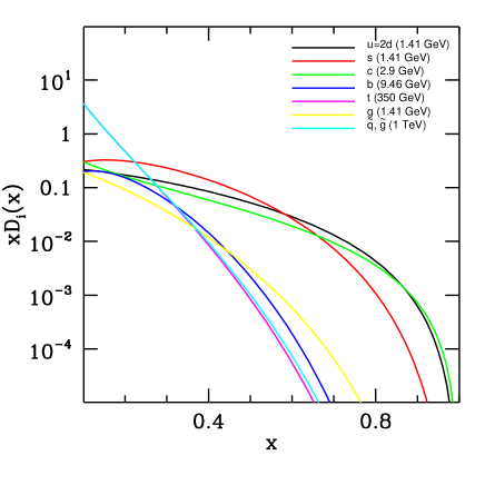
Figure 3.7: The fragmentation functions of Table 3.2 for the different partons.

The fragmentation functions after beeing evolved to high scales can be well parametrized as:

$$D(x)=N_{1}x^{\alpha_{1}}(1-x)^{\beta_{1}}+N_{2}x^{\alpha_{2}}(1-x)^{\beta_{2}}.$$ (3.14)

Table 3.3 gives the fragmentation functions averaged over the quark flavors for the energy range $10^{12}$ eV-$10^{17}$ eV in this parametrization.

log(Q/eV)	$N_{1}$	$\alpha_{1}$	$\beta_{1}$	$N_{2}$	$\alpha_{2}$	$\beta_{2}$
SM
12.	0.0186	-1.28	3.56	0.199	-1.70	5.26
13.	0.0194	-1.30	3.66	0.186	-1.71	5.36
14.	0.0207	-1.31	3.76	0.175	-1.72	5.47
15.	0.0215	-1.32	3.84	0.165	-1.73	5.56
16.	0.0225	-1.35	3.93	0.157	-1.74	5.66
17.	0.0232	-1.35	4.01	0.150	-1.75	5.75
MSSM
12.	0.026	-1.37	4.23	0.106	-1.77	6.03
13.	0.027	-1.39	4.41	0.0941	-1.79	6.30
14.	0.028	-1.22	4.57	0.0890	-1.80	6.51
15.	0.028	-0.735	4.70	0.0855	-1.80	6.48
16.	0.029	-0.421	4.85	0.0785	-1.81	6.55
17.	0.030	-0.441	5.00	0.0724	-1.82	6.76

Table 3.3: The fragmentation functions of the proton averaged over the quark flavors for high energies in the SM and MSSM using the parametrization $D(x)=N_{1}x^{\alpha_{1}}(1-x)^{\beta_{1}}+N_{2}x^{\alpha_{2}}(1-x)^{\beta_{2}}$

The FFs obtained this way are not accurate for very small $x$ values, since even the original FFs are not well known in this region.

At small $x$ values multiple soft gluon emission can be described by the MLLA [66]. This gives the shape of the total hadronic FF for soft particles (not distinguishing individual hadronic species)

$$xF(x,Q^{2})\propto\exp\left[-\ln(x/x_{m})^{2}/(2\sigma^{2})\right],$$ (3.15)

which is peaked at $x_{m}=\sqrt{\Lambda/Q}$ with $2\sigma^{2}=A\ln^{3/2}(Q/\Lambda)$. According to [60] the values of $A$ are $\sqrt{7/3}/6$ and $1/6$ for SM and MSSM, respectively. The MLLA describes the observed hadroproduction quite accurately in the small $x$ region [79]. For large values of $x$ the MLLA should not be used.

We smoothly connected the solution for the FF obtained by the DGLAP equations and the MLLA result at a given $x_{c}$ value. Our final result on $m_{X}$ is rather insensitive to the choice of $x_{c}$, the uncertainty is included in our error estimate. The SP decay also produces a huge number of pions. The total number of produced pions is essential since they decay to photons which loose most of their energy during propagation and give a contribution to the low energy photon spectrum. Thus we also determined the FF of the pion. Figure 3.8 shows the FF for the proton and pion at $Q=10^{16}$ GeV in SM and MSSM.

Figure 3.8: The FFs averaged over the quark flavors at $Q=10^{16}$ GeV for proton/pion in SM (solid/dotted line) and in MSSM (dashed/dashed-dotted line) in the relevant $x$ region. To show both the small and large $x$ behavior we change from logarithmic scale to linear at $x=0.01$.

3.2.2 Comparison of the predicted and the observed spectra

UHECR protons produced in the halo of our galaxy can propagate practically unaffected and the production spectrum should be compared with the observations.

Particles of extragalactic origin and energies above $\approx 5\cdot 10^{19}$ eV loose a large fraction of their energies due to interactions with CMBR [26]. This effect can be quantitatively described by the function $P(r,E,E_{c})$ introduced and calculated in section 3.1.2. The original UHECR spectrum is changed at least by two different ways: (a) there should be a steepening due to the GZK effect; (b) particles loosing their energy are accumulated just before the cutoff and produce a bump. We studied the observed spectrum by assuming a uniform source distribution for UHECRs.

Our analysis includes the published and the unpublished UHECR data of [27, 28, 29, 31]. Due to normalization difficulties we did not use the Yakutsk [30] results. We also performed the analysis using the AGASA data only and found the same value (well within the error bars) for $m_{X}$. Since the decay of SPs results in a non-negligible flux for lower energies $\log(E_{min}/\mbox{eV})=18.5$ was used as a lower end for the UHECR spectrum. Our results are insensitive to the definition of the upper end (the flux is extremely small there) for which we chose $\log(E_{max}/\mbox{eV})=26$. As it is usual we divided each logarithmic unit into ten bins. The integrated flux gives the total number of events in a bin. The uncertainties of the measured energies are about 30% which is one bin. Using a Monte-Carlo method we included this uncertainty in the final error estimates. The predicted number of events in a bin is given by

$$N(i)=\int_{E_{i}}^{E^{i+1}}\left[A\cdot E^{-3.16}+B\cdot j(E,m_{X})\right],$$ (3.16)

where $E_{i}$ is the lower bound of the $i$-th energy bin. The first term describes the data below $10^{19}$ eV according to [27], where the SP decay gives negligible contribution. The second one corresponds to the spectrum of the decaying SPs. A and B are normalization factors.

Figure 3.9: The available UHECR data with their error bars and the best fit from a decaying SP using the EG-MSSM scenario. Note that there are no events above $3\times 10^{20}$ eV (shown by an arrow). Nevertheless the experiments are sensitive even in this region. Zero event does not mean zero flux, but a well defined upper bound for the flux (given by the Poisson distribution). Therefore the experimental value of the integrated flux is in the ”hatched” region with 68% confidence level. (”hatching” is a set of individual error bars; though most of them are too large to be depicted in full) Clearly, the error bars are large enough to be consistent with the SP decay.

The expectation value for the number of events in a bin is given by eqn. (3.16) and it is Poisson distributed. To determine the most probable $m_{X}$ value we used the maximum-likelihood method by minimizing the $\chi^{2}(A,B,m_{X})$ for Poisson distributed data [64]

$$\chi^{2}=\sum_{i=18.5}^{26.0}2\left[N(i)-N_{o}(i)+N_{o}(i)\ln\left(N_{o}(i)/N(i)\right)\right],$$ (3.17)

where $N_{o}(i)$ is the total number of observed events in the $i$-th bin. In our fitting procedure we had three parameters: $A,B$ and $m_{X}$. The minimum of the $\chi^{2}(A,B,m_{X})$ function is $\chi^{2}_{min}$ at $m_{Xmin}$ which is the most probable value for the mass, whereas $\chi^{2}(A^{\prime},B^{\prime},m_{X})\equiv\chi^{2}_{o}(m_{X})=\chi^{2}_{min}+1$ gives the one-sigma (68%) confidence interval for $m_{X}$. Here $A^{\prime},B^{\prime}$ are defined in such a way that the $\chi^{2}(A,B,m_{X})$ function is minimized in $A$ and $B$ at fixed $m_{X}$. Figure 3.9 shows the measured UHECR spectrum and the best fit in the EG-MSSM scenario. The first bump of the fit represents particles produced at high energies and accumulated just above the GZK cutoff due to their energy losses. The bump at higher energy is a remnant of $m_{X}$. In the halo models there is no GZK bump (Figure 3.10), so the relatively large $x$ part of the FF moves to the bump around $5\times 10^{19}$ GeV resulting in a much smaller $m_{X}$ than in the extragalactic case. An interesting feature of the GZK effect is that the shape of the produced GZK bump is rather insensitive to the injected spectrum so the dependence of $\chi^{2}$ on the choice of the FF is small. The experimental data is far more accurately described by the GZK effect (dominant feature of the extragalactic fit) than by the FF itself (dominant for halo scenarios).

Figure 3.10: The available UHECR data with their error bars and the best fit using the halo-MSSM scenario.

3.2.3 Predictions for $m_{X}$

To determine the most probable value for the mass of the SP we studied four scenarios. Table 3.4 and Figure 3.11 contain the $\chi^{2}_{min}$ values and the most probable masses with their errors for these scenarios.

The UHECR data favors the EG-MSSM scenario. The predicted mass is $10^{b}$ GeV, where $b=14.6_{-1.7}^{+1.6}$. The goodnesses of the fits for the halo models are far worse. The SM and MSSM cases do not differ significantly. The most important message is that the masses of the best fits (extragalactic cases) are compatible within the error bars with the MSSM gauge coupling unification GUT scale [80].

scenario	$\chi^{2}$	$\log_{10}(m_{X}/\mbox{GeV})$
halo-SM	24.9	$11.98^{+.15}_{-.12}$
halo-MSSM	25.0	$12.04^{+.15}_{-.12}$
EG-SM	16.6	$14.2^{+1.4}_{-1.5}$
EG-MSSM	16.5	$14.6^{+1.6}_{-1.7}$

Table 3.4: The $\chi^{2}$ and $m_{X}$ values for the four scenarios.

Figure 3.11: The most probable values for the mass of the decaying ultra heavy dark matter with their error bars and the total $\chi^{2}$ values. Note that 21 bins contain nonzero number of events and eqn.(3.16) has 3 free parameters.

The SP decay will also produce a huge number of pions which will decay into photons. Our spectrum contains 94% of pions and 6% of protons. This $\pi/p$ ratio is in agreement with the calculations of [81, 33] which showed that for different classes of models with $m_{X}\mathop{\raise 1.29167pt\hbox{$<$\kern-7.5pt\raise-4.73611pt\hbox{$\sim$}}}10^{16}$ GeV , which is the upper boundary of our confidence intervals, the generated gamma spectrum is still consistent with the observational constraints.

In the near future the UHECR statistics will probably be increased by an order of magnitude [51]. Performing our analysis for such a hypothetical statistics the uncertainty of $m_{X}$ was found to be reduced by two orders of magnitude.

Since the decay time of the SPs should be at least the age of the universe it might happen that such SPs overclose the universe. Due to the large mass of the SPs a single decay results in a large number of UHECRs, thus a relatively small number of SPs can describe the observations. We calculated the minimum density required for the best-fit spectrum in each scenario and it was more than ten orders of magnitude smaller than the critical one.

Chapter 4 The Poor Man’s Supercomputer

In this chapter I briefly describe the hardware and software architecture of the Poor Man’s Supercomputer (PMS) built at the Eötvös University [82]. This supercomputer was used to perform the lattice simulations of chapter 2 as well as the Monte-Carlo analysis of chapter 3.

Our purpose was to build a high performance supercomputer from PC elements. We use PC’s for two reasons. They have excellent cost/performance ratios [83] and can easily be upgraded when faster motherboards and CPUs will be available.

The PMS project started in 1998, and the machine has been ready for physical calculations since the spring of 2000. Our first PMS machine (PMS1) consists of 32 PC’s arranged in a three-dimensional $2\times 4\times 4$ mesh. Each node has two special communication cards providing fast communication through flat cables to the six neighbours. This gives a much better performance than one Ethernet Token Ring.

The following sections describe the hardware and software architectures of PMS. First a short overview of the machine is given and then the hardware and the software aspects are described in more details. Some performance results are also presented.

4.1 Overview

The nodes in PMS are based on PC components. Our first PMS machine (PMS1) contains 32 rack-mounted nodes. Each node is powered by its own standard PC power supply located at the bottom of the rack.

Each node in PMS is an almost complete PC. In PMS1 the current configuration of a node consists of a 100MHz motherboard (SOYO SY-5EHM), a single 450MHz AMD K6-II processor, 128MB (7ns) SDRAM, 10Mb Ethernet card, and a hard disk of capacity 2.1 Gbyte. The nominal speed of each node is 225 Mflops, since floating point operations of the AMD processor require two clock cycles.

PMS uses special hardware for communication (PMS CH) to make high speed parallel calculations possible. The basic idea behind the hardware is that the PMS CH provides each node with direct connection to its nearest neighbors. Our first implementation of the PMS CH includes two plug-in ISA cards, the PMS CPU card and the PMS Relay card. The PMS CH handles both polled port (PP) IO operations and direct memory access (DMA) between two selected nodes. However, DMA is not used at present.

Programming the PMS CH is a fairly simple task. It is currently done under Linux. All low-level device drivers are written in C and the programmer may use all kinds of commercial, share-ware or free-ware compilers. Using the communication drivers requires only the knowledge of a few functions.

The nodes are arranged in a $2\times 4\times 4$ mesh as shown in Figure 4.1. In each node both the PMS CPU and the PMS Relay cards are installed providing fast communication to the six nearest neighbors. At the boundaries periodic boundary conditions are realized as indicated in Figure 4.1, where the links at the boundaries correspond to the ones on the other sides. This determines the hardware architecture of the machine, which is similar to that of the APE machines [84].

Figure 4.1: The PMS cluster

Debian Linux 2.1 is installed on each node. After turning the power on each node boots from its own hard-disk. All nodes can be accessed through the Ethernet Token Ring. There is a main computer that controls the whole cluster. A tiny job-management system was written to copy the executable program code and the appropriate data to and from the nodes, to execute the programs and to collect the results. In principle, the Ethernet Token Ring could be used for data transfer between the nodes during simulations. However, this turned out to be too slow in most cases. One major reason for this is that any data transfer between two machines makes the whole network busy. Since building up the Ethernet connection (protocol overhead) is quite slow even for two computers, the Ethernet Token Ring is not satisfactory.

The special communication cards –described in more detail in the next section– provide faster communication between adjacent nodes. However, this makes the machine applicable only to local problems, where communication between the neighboring nodes is necessary. In PMS1 the speed of communication through these cards –limited essentially by the ISA bus speed– is about 2 MB/s. The measured value in real applications , i.e. the speed of a link for a given direction is essentially the same: 2.2MB/s. The time needed to build up our communication is negligible for package sizes over 1kB. Furthermore, 16 pairs of machines can simultaneously communicate. The system is scalable. One can build machines with larger number of nodes. The total inter-node communication performance is proportional to the number of nodes.

4.2 Description of the PMS Communication
Hardware (CH)

There are two communication cards in each machine. The CPU card contains the main circuits needed for transmitting data, while the Relay card contains the connectors for the flat cables connecting the adjacent nodes and some additional circuits.

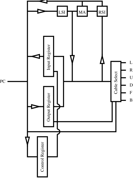
Figure 4.2: The PMS communication card

The block diagram of the cards is shown in Figure 4.2. The circuits of both cards are included. There are two 16-bit buffers, the output buffer and the input buffer, which accept the data coming from the computer and from one of the adjacent nodes, respectively. The Control Register is used –among other things– to clear the buffers and set the node to either sender or receiver state. The Cable Select circuit selects which direction the data is sent to or received from. The six directions are labeled as left (L), right (R), up (U), down (D), front (F), back (B). If the same physical cable is selected by two adjacent nodes, one of them being set as sender and the other as receiver, a physical connection is established and the content of the output register of the sender is immediately transferred to the receiver’s input register. The Local State Indicator (LSI) and the Remote State Indicator (RSI) are two registers to indicate the states of the nodes. There are 12 LSI and 12 RSI lines. They correspond to sending to and receiving from the six directions. Each node can indicate its request for sending or receiving through the LSI lines. The RSI lines are identical to the six neighbors’ LSI lines. If there is a match between RSI and LSI signals (i.e. a send and a corresponding receive request coincide) then the Match Any (MA) bit is set and an IRQ is generated on the PC bus. The interrupt is generated on both nodes at the same time, so the interrupt handlers on both machines can safely start transferring data without any extra synchronization. The data can be transferred either by DMA (not used at present) or by consecutive I/O operations.

The Cable Select circuit, the LSI, RSI and MA registers together with the flat cable connectors are located on the relay card, while all other circuits are located on the CPU card.

4.3 Software

As mentioned above, the whole cluster is connected via an Ethernet Token Ring. Each node has a special hostname that corresponds to its location in the cluster. The hostnames are s000,s001,s002,s003,s010 $\dots$ s133. The numbers in the hostname correspond to the coordinates of the node in the three dimensional mesh. When it is necessary for a node to identify itself (e.g. write/read priorities during inter-node communication, see below) the file ’/etc/hostname’ is used. The Ethernet Token Ring is used only for job management, i.e. to distribute and collect data to and from the nodes. It is not used for inter-node communication during simulations. This is achieved by the special hardware described in the previous section.

In order to take advantage of the fast communication from applications (e.g. high level C, C++ or Fortran code), a low-level Linux kernel driver has been developed to access all the registers of the communication card. From the user level cards can simply be reached by reading or writing the device files ’/dev/pms0, /dev/pms1 … /dev/pms5’. The six device files correspond to the six directions. A write operation to one of these device files will transmit data to the corresponding direction, and reading from these device files reads out previously transferred data. All the necessary input/output operations for transferring data blocks are performed by the device driver. Notice the important feature that this can be reached from any high level C, C++, Fortran code for which compilers are available.

The main structure of the device driver is similar to that of the card. There are six read buffers, one for each direction in the main memory of the machine and there is one write buffer. The data are always written to the write buffer and read out from one of the read buffers.

The driver has two main parts. The first part is accessed from applications when the user writes or reads any of the device files ’/dev/pms*’. The other part is the interrupt handler where the real data transfer takes place.

Whenever data are written to one of the device files, all the driver does is to copy the written data to the write buffer and set the corresponding LSI send signal to indicate that a data send is requested. If the buffer is already full, an error byte is returned to the application. Reading from the device files is similar: if there are data in the corresponding read buffer, they are sent to the application and the LSI receive line is set, since the node is ready to receive new data. If the read buffer is empty, an ’End Of File’ byte is returned to the application.

When there is a coincidence between corresponding LSI and RSI signals, an interrupt is generated by the card, which invokes the driver’s interrupt handler. It is the task of the handler to transfer data from the sender to the receiver. The interrupt handlers on the two communicating nodes start almost at the same time. The difference may only be a few clock cycles. There is, however, a need for synchronization. If the machines are ready to send or receive the first byte they indicate it with their LSI lines. Notice that this will not cause an extra interrupt since interrupts are disabled within the interrupt handler. The sender first transmits the size of the package that will follow in 16-bit words. In the present version this is a 16-bit value, so the maximum size of a package that can be transferred is 128 kbytes. Then the given number of 16-bit values follow. Each word from the sender’s write buffer is copied to the receiver’s read buffer. Finally, a 32-bit checksum is sent. The receiver computes its own checksum and if it does not match the received checksum, it is indicated to the sender and the whole transfer is repeated. The final step in the interrupt handler is to clear the LSI lines of both nodes. On the one hand this indicates for the sender that the data have been transferred and the write buffer is empty again. On the other hand this tells the receiver that the corresponding read buffer is full, so no new data can arrive unless the buffer is emptied.

The buffer sizes are set in the driver to constant values. From the previous paragraph it is clear that the maximum reasonable buffer size is 128 kbytes. In order to save memory, while allowing large packages at the same time the buffer size is set to only 64 kbytes at present.

The driver makes application programming quite easy. Communication can be achieved by accessing the above mentioned device files. However, some C functions have also been written to make writing applications even simpler. These functions are the following:

pms_open is used to initialize the card. It clears all buffers, sets the LSI receive lines, clears the LSI send lines and enables interrupts. The node thus becomes ready to receive data from any of the neighbors.

pms_close is used to close the card. All LSI lines are cleared and interrupts are disabled. No further communication may take place after this function call.

pms_send, pms_recv are used to send and receive data. Their parameters are the direction, the number of bytes to send, and a pointer to the beginning of the data. On success they return a positive value, otherwise a negative one. If there is no data in the read buffer, pms_recv returns 0.

pms_send_receive is a commonly used combination of pms_send and pms_recv. It sends data to the specified direction and receives data from the opposite direction. The order of send and receive depends on the parity of the node as discussed later.

pms_collect, pms_average are global operations that simply collect or take the average of data from all nodes in one direction.

The driver does not take care of any priority problems. It is possible to write applications that will not work since all nodes are waiting for data while none of them is sending anything. This is often the case when the same code is running on all the nodes without any priority check. There is a simple solution to these kind of problems. The parity of the node is simply the parity of the sum of the three digits in its hostname. Each time when communication is performed, even nodes send data first and receive afterwards, while odd nodes receive first and send their data afterwards. This simple method is used in the pms_send_receive function. Applications that use only this function to transfer data should not worry about priority problems.

4.4 Performance

The lattice simulations of chapter 2 were carried out on our parallel computer PMS1. We also measured the performance of the machine with a much simpler pure SU(3) gauge theory. The most CPU time consuming parts, manipulation with $2\times 2$ and $3\times 3$ complex matrices, were written in assembly language. This increased the speed of the codes by about a factor of two.

We obtained similar results for the speed of the code and for the communication between nodes in the two cases. The MSSM results for communication are actually somewhat better. The reason for that is quite simple. The number of variables in the MSSM is larger by a factor of two than in pure SU(3) gauge theory; however, the number of floating point operations needed for a full update is more than an order of magnitude larger. Thus, for the same lattice size the time needed to transfer the surface variables –done by the communication cards– compared to the update time is smaller for MSSM than for the pure SU(3) theory. We estimated that a similar or a bit less speed than in SU(3) gauge theory should be observed for fermionic systems with multiboson [85] algorithms.

For small lattice sizes the most economical way to use our 32 PC cluster is to put independent lattices on the different nodes. The maximum lattice size in the SU(3) theory for 128 MB memory is $\sim 20^{4}$, or for finite temperature systems $6\cdot 32^{3}$. One thermalizes such a system on a single node, then distributes the configuration to the other nodes and continues the updating on all 32 nodes. We measured the sustained performance of the cluster in this case, which gave $32\times 152$Mflops=4.9Gflops. This 152Mflops/node performance means that one double precision operation is carried out practically for every third clock cycle of the 450 MHz, whereas the nominal maximum of the processor is one operation for every second clock cycle. As it was mentioned above, without assembly programming an approximate reduction factor of two in the performance was observed.

Increasing the volume of the simulated system one can divide the lattice between 2 nodes (the $2\times 4\times 4$ topology has 2 nodes in one of the directions). For even larger lattices one can use 4 nodes (4 in one direction), 8 nodes ($2\times 4$ in two directions) 16 nodes ($4\times 4$ in two directions) or 32 nodes ($2\times 4\times 4$ in three directions). Again, the most economical way to perform the simulations is to prepare one thermalized configuration and put it on other nodes (this method obviously can not be used for the $2\times 4\times 4$ topology, because in this case the whole machine with 32 nodes is just one lattice).

Based on our measurements we determined the sustained performance of a 32-node PMS cluster as a function of the lattice volume. The result for a set of lattice volumes for finite temperature systems with temporal extension, $L_{t}=6$ for SU(3) and $L_{t}=4$ for MSSM can be seen on Figure 4.3. Clearly, the largest volume one can reach is approximately twice as large for the SU(3) gauge theory than for the MSSM. For both cases there are regions where the performance increases with the volume. This can be easily understood to happen due to the fact that larger volume means better surface/volume ratio, thus better performance. There are three drops in the performance for both SU(3) and MSSM. They correspond to lattice volumes for which new communication directions were opened (or, in other words, the dimension of the mesh of the nodes on which the lattice was divided, increased by one) in order to fit the lattice into the available RAMs. As it can be seen the performance for the MSSM is still very high even at the largest volume with three-dimensional communication: it is just 10% smaller than the performance without communication. This plot gives us the optimum architecture of such a parallel computer. The number of nodes and the number of communication directions used for a given lattice should be as small as possible simultaneously. This means a $2\times 4\times 4$ topology for 32 nodes and a $2\times 4\times 8$ topology 64 nodes.

Figure 4.3: Sustained performance of PMS1 as a function of the lattice volume for pure SU(3) gauge theory and for MSSM. The endpoints of the lines correspond to the largest volumes which can be simulated on a 32 PC cluster.

Despite the fact that the speed of the communication between two nodes is not that high (2 Mb/s) the performance of the cluster is quite good. The reason for this is the high speed of the individual nodes (450 MHz) and the large RAM on each node. This sort of design does not need a division of the lattice to hundreds of sub-lattices, thus it does not need a very fast communication.

The total sustained performance of PMS1 for double precision calculations is $\approx$4Gflops. The price/(sustained performance) ratio is quite excellent:$3/Mflops.

For single precision simulations one can use the MMX instruction set which is 8 times faster than the double precision operations (4 operations for each clock cycle). We estimated the single precision performance by assuming that MMX programming results in 20% decrease in performance. The total performance of PMS1 is $\approx$20Gflops with 0.60$/Mflops price-to-sustained performance ratio. The PMS1 machine, similarly to other workstation farms has a moderate maximum sustained performance as compared to Teraflop-scale machines (CP-PACS [86] or QCDSP [87]). However, PMS1 has a much better price/(sustained performance) ratio than other workstation farms.

Chapter 5 SUMMARY

In my thesis two phenomena pointing beyond the Standard Model were discussed. In chapter 2 the possibility of baryogenesis in the minimal supersymmetric extension of the Standard Model was examined. The problem cannot be solved fully by perturbation theory so lattice simulations were needed. My main contribution to this analysis is related to this non-perturbative part.

A 5000 line C program was written that performs simulations of the MSSM. During the writing of this program the Monte-Carlo methods used in earlier works had to be improved. The overrelaxation and heatbath algorithms for the scalar fields were introduced in section 3.1.2.

Using the MSSM program, systematic finite temperature and zero temperature simulations were performed. First the phase transition point was determined at finite temperature for different volumes and infinite volume extrapolation was carried out. Then at the same physical point zero temperature simulations were performed and the mass spectrum was determined. This whole procedure was repeated for four different lattice spacings.

After observing the good agreement with perturbation theory, the lattice results obtained at different lattice spacings can be perturbatively corrected to be on a line of constant physics (LCP) and continuum limit extrapolation can be done.

For perturbation theory it is important to know the renormalization corrections to the squark masses. To this end the phase diagram in the $m_{U}^{2}$–$T$ plane was determined. The transition point to the color-breaking phase is a good reference point for squark mass renormalization.

The produced baryon number is in strong connection with the shape of the bubble wall during the phase transition. Using constrained simulation, the profile of the bubble wall can be measured. With an appropriate shifting procedure the wall profile and the wall width were determined. The variation of the $\beta$ parameter through the bubble wall was also found.

The other phenomenon which was discussed in chapter 3 is connected to ultrahigh energy cosmic rays. The highest energy cosmic rays have macroscopic energy which cannot be explained with our present knowledge. The interesting clustering features of the highest energy events lead to the assumption that these ultrahigh energy cosmic rays may come from compact sources. Based on the observed clustering properties the density of these sources was determined for arbitrary spatial, energy and luminosity distributions. Three examples for energy distribution and two for luminosity distribution were studied in detail.

A useful function of the analysis was the $P(r,E,E_{c})$ probability function which gives the probability that a proton starting with energy $E$ has its energy above $E_{c}$ after traveling a distance of $r$. With a Monte-Carlo analysis this function was computed for a wide range of parameters. Thus using this parametrization the observed spectrum can be calculated to any injected spectrum without further Monte-Carlo simulations.

The fact that some events have extremely high energies gives the possibility that they might not be accelerated from lower energies (these are the so called ”bottom-up” scenarios), but they are the decay products of some heavy metastable particle. These scenarios are commonly called ”top-down” scenarios.

Based on this assumption the decay spectrum of superheavy particles was determined. For this the fragmentation functions of protons at these high energies were needed. Since this is a non-perturbative quantity, the experimental results for the fragmentation functions at low energy had to be used and these were evolved to high energies. This fragmentation function was combined with the prediction of the Modified Leading Logarithmic Approximation (MLLA) which gives the small momentum region of the fragmentation functions more accurately.

The lattice simulations of MSSM and the Monte-Carlo study of the propagation of cosmic rays required a huge amount of CPU time. We decided to build a cost-effective supercomputer from PC elements, the Poor Man’s Supercomputer (PMS). In the fourth chapter of my thesis the hardware and software architecture of this machine was described. The most important hardware solution is the special communication card that provides fast communication between adjacent nodes, while on the software side the job-management system and the kernel driver for the cards were designed.

5.1 Acknowledgments

First of all I would like to thank the help and patience of my advisor Zoltán Fodor. He has a great part in my results with lots of ideas and encouragement. I am also grateful to Ferenc Csikor for many useful discussions. It was a pleasure to work together with Pál Hegedüs, Viktor Horváth, Antal Jakovác and Attila Piróth. Finally I thank B.A Kniehl for the fragmentation function of the proton generously supplied prior to its publication.

Bibliography

- [1] H. N. Brown et al. [Muon g-2 Collaboration], Phys. Rev. Lett. 86, 2227 (2001).
- [2] A. G. Cohen, A. De Rujula, S. L. Glashow, Astrophys. J. 495 (1998) 539.
- [3] A. D. Sakharov, JETP Letters 91B, 24 (1967).
- [4] V. A. Kuzmin, V. A. Rubakov and M. E. Shaposhnikov, Phys. Lett. B155 36 (1985).
- [5] P. Arnold and O. Espinosa, Phys. Rev. D47, 3546 (1993), erratum ibid., D50, 6662 (1994); W. Buchmüller et al., Ann. Phys. (NY) 234, 260 (1994); Z. Fodor and A. Hebecker, Nucl. Phys. B432, 127 (1994); W. Buchmuller, Z. Fodor and A. Hebecker, Nucl. Phys. B447, 317 (1995).
- [6] K. Farakos et al., Nucl. Phys. B425, 67 (1994); A. Jakovác and A. Patkós, Nucl. Phys. B494, 54 (1997);A. Jakovac, K. Kajantie and A. Patkos, Phys. Rev. D49, 6810 (1994); A. Jakovac and A. Patkos, Phys. Lett. B334, 391 (1994).
- [7] B. Bunk et al., Nucl. Phys. B403, 453 (1993), Z. Fodor et al., Phys. Lett. B334, 405 (1994); Nucl. Phys. B439, 147 (1995), F. Csikor et al., Nucl. Phys. B474, 421 (1996).
- [8] Z. Fodor et al., Nucl. Phys. B439, 147 (1995).
- [9] K. Kajantie et al., Nucl. Phys. B407, 356 (1993); Nucl. Phys. B466, 189 (1996); O. Philipsen et al., Nucl. Phys. B469, 445 (1996).
- [10] F. Karsch, T. Neuhaus, A. Patkos and J. Rank, Nucl. Phys. B (Proc. Suppl.) 53, 623 (1997); K. Kajantie et al., Phys. Rev. Lett. 77, 2887 (1996); M. Gürtler et al., Phys. Rev. D56, 3888 (1997).
- [11] F. Csikor et al., Phys. Rev. Lett. 82, 21 (1999) (for analytical end point results see second paper of [5] and W. Buchmüller, O. Philipsen, Nucl. Phys. B443 47 (1995)); F. Csikor, Z. Fodor, P. Hegedüs and A. Piróth, Phys. Rev. D 60, 114511 (1999).
- [12] G. F. Guidice, Phys. Rev. D45, 3177 (1992); J. R. Espinosa et al., Phys. Lett. B307, 106 (1993); A. Brignole et al., Phys. Lett. B324, 181 (1994); J. R. Espinosa, Nucl. Phys. B475, 273 (1996); B. de Carlos, J. R. Espinosa, Nucl. Phys. B503, 24 (1997); D. Bödeker et al., Nucl. Phys. B497, 387 (1997); J. M. Cline, G. D. Moore, Phys. Rev. Lett. 81, 3315 (1998); M. Carena, M. Quiros and C. E. Wagner, Nucl. Phys. B 524, 3 (1998); M. Losada, Nucl. Phys. B537, 3 (1999); hep-ph/9905441.
- [13] M. Carena et al., Phys. Lett. B380, 81 (1996); Nucl. Phys. B524 3 (1998).
- [14] M. Laine, K. Rummukainen, Phys. Rev. Lett. 80 5259 (1998); Nucl. Phys. B535 423 (1998).
- [15] K. Funakubo et al., Prog. Theor. Phys. 99 1045 (1998); ibid., 102 389 (1999); M. Laine, K. Rummukainen, Nucl. Phys. B545 141 (1999); hep-lat/9908045.
- [16] F. Csikor, Z. Fodor, P. Hegedüs, A. Jakovác, S. D. Katz, A. Piróth, Phys. Rev. Lett. 85, 932 (2000)
- [17] G. D. Moore, Nucl. Phys. B523, 569 (1998).
- [18] P. Huet, A. E. Nelson, Phys. Rev. D53, 4578 (1996); Phys. Lett. B355, 229 (1995); M. Carena et al., Nucl. Phys. B503, 387 (1997); A. Riotto, Nucl. Phys. B518, 339 (1998); Phys. Rev. D58 095009 (1998); N. Rius, V. Sanz, hep-ph/9907460; M. Brhlik, et al., hep-ph/9911243.
- [19] A. M. Ferrenberg and R. H. Swendsen, Phys. Rev. Lett. 61, 2635 (1988), Phys. Rev. Lett. 63, 1195 (1989).
- [20] C. N. Yang and T. D. Lee, Phys. Rev. 87, 404 (1952); T. D. Lee and C. N. Yang, Phys. Rev. 87, 410 (1952).
- [21] G. Bhanot, S. Black, P. Carter and R. Salvador, Phys. Lett. B 183, 331 (1987); G. Bhanot, K. Bitar, S. Black, P. Carter and R. Salvador, Phys. Lett. B 187, 381 (1987); B. A. Berg and T. Neuhaus, Phys. Lett. B 267, 249 (1991).
- [22] F. Csikor, Z. Fodor, T. Herpay, V.K. Horváth, A. Jakovác, S. D. Katz, in preparation.
- [23] J. M. Cline et al., Phys. Rev. D60, 105035 (1999).
- [24] D. Jasnow, Rep. Prog. Phys. 47, 1059 (1984)
- [25] J. M. Moreno et al., Nucl. Phys. B526, 489 (1998); P. John, Phys. Lett. B452, 221 (1999).
- [26] K.Greisen, Phys.Rev.Lett. 16, 748 (1966); G.T.Zatsepin, V.A.Kuzmin, Pisma Zh.Exp.Teor.Fiz. 4, 114 (1966).
- [27] M. Takeda et al., Phys. Rev. Lett. 81, 1163 (1998); astro-ph/9902239; www-akeno.icrr.u-tokyo.ac.jp/AGASA/
- [28] D.J. Bird et al., Phys. Rev. Lett. 71, 3401 (1993); Astrophys J. 424, 491 (1994); ibid 441, 144 (1995).
- [29] M.A. Lawrence, R.J.O. Reid and A.A. Watson, J. Phys. G17, 773 (1991).
- [30] N.N. Efimov et al., "Proc. Astrophysical Aspects of the Most Energetic Cosmic Rays", p. 20, eds. M. Nagano and F. Takahara, World Sci., Singapore, 1991.
- [31] D. Kieda et al., to appear in Proc. of the 26th ICRC, Salt Lake, 1999; www.physics.utah.edu/Resrch.html
- [32] S. Yoshida, M. Teshima, Prog. Theor. Phys. 89, 833 (1993); F.A. Aharonian, J.W. Cronin, Phys. Rev. D50, 1892 (1994); R.J. Protheroe, P. Johnson, Astropart. Phys. 4, 253 (1996).
- [33] P. Bhattacharjee and G. Sigl, Phys. Rep. 327, 109 (2000).
- [34] A. Achterberg et al., astro-ph/9907060.
- [35] T. Stanev et al., astro-ph/0003484.
- [36] G. Domokos, S. Nussinov, Phys. Lett. B187, 372 (1987); D. Fargion, B. Mele, A. Salis, Astrophys. J. 517, 725 (1999); T.J. Weiler, Astropart. Phys. 11 303 (1999), Astropart. Phys. 12, 379 (2000) (Erratum); G. Domokos, S. Kövesi-Domokos, Phys. Rev. Lett. 82, 1366 (1999).
-
[37]
G.R. Farrar and T. Piran, Phys. Rev. Lett.
84, 3527 (2000);
A. Dar, astro-ph/0006013. - [38] N. Hayashida et al., Phys. Rev. Lett. 77, 1000 (1996).
- [39] Y. Uchihori et al., Astropart. Phys. 13, 151 (2000).
- [40] Z. Fodor and S. D. Katz, Phys. Rev. D 63, 023002 (2001).
- [41] S.L. Dubovski, P.G. Tinyakov, JETP Lett. 68, 107 (1998); V.Berezinsky, A.A. Mikhailov, Phys. Lett. B449, 61 (1999); C.A. Medina Tanco, A.A. Watson, Astrop. Phys. 12, 25 (1999).
- [42] K. Mannheim, Astropart. Phys. 3, 295 (1995).
- [43] J.P. Rachen, P.L. Biermann, Astron. Astrophys. 272, 161 (1993).
- [44] J.W. Elbert, P. Sommers, Astrophys. J. 441, 151 (1995).
- [45] P.L. Biermann, P.A. Strittmatter, Astrophys. J. 322, 643 (1987).
- [46] C.T. Hill, D.N. Schramm, T.P. Walker, Phys. Rev. D36, 1007 (1987); P. Bhatacharjee, C.T. Hill, D.N. Schramm, Phys. Rev. Lett. 69, 56 (1992); G. Sigl astro-ph/9611190; V. Berezinsky, A. Vilenkin, astro-ph/9704257.
- [47] V.S. Berezinsky, S.I. Grigorieva, in Proc. of the 16th Int. Cosmic Ray Conf., Kyoto 1979, Vol. 2. p. 81.
- [48] R.D. Blandford, Phys. Scr. T85, 191 (2000).
- [49] Z. Fodor and S. D. Katz, Phys. Rev. Lett. 86, 3224 (2001).
- [50] S.L. Dubovsky, P.G. Tinyakov and I.I. Tkachev, Phys. Rev. Lett. 85, 1154 (2000).
- [51] M. Boratav, Nucl. Phys. Proc. 48, 488 (1996); C.K. Guerard, ibid 75A, 380 (1999); X. Bertou, M. Boratav, A. Letessier-Selvon, astro-ph/0001516.
-
[52]
X. Bertou, M. Boratav, A. Letessier-Selvon,
Int. J. Mod. Phys. A15, 2181 (2000). - [53] J.N. Bahcall and E. Waxman, hep-ph/9912326.
- [54] J. Ellis et al., Phys. Lett. B247, 257 (1990); Nucl. Phys. B373, 399 (1992); P. Gondolo, G.B. Gelmini, S. Sarkar, Nucl. Phys. B392, 111 (1993).
- [55] V. Berezinsky, M. Kachelrieß and A. Vilenkin, Phys. Rev. Lett. 79, 4302 (1997);
- [56] M. Birkel and S. Sarkar, Astropart. Phys. 9, 297 (1998).
- [57] K. Benakli et al., Phys. Rev. D59, 047301 (1999).
- [58] P. Blasi and R. Sheth, Phys.Lett. B486, 233 (2000).
- [59] C.T. Hill, Nucl. Phys. B224, 469 (1983).
- [60] V.Berezinsky, M.Kachelrieß, Phys.Lett. B434, 61 (1998).
- [61] P.L. Schechter, Astrophys. J. 203, 297 (1976).
-
[62]
E. Waxman, K.B. Fisher and T. Piran, Astrophys. J. 483,
1 (1997);
M. Giller, J. Wdowczyk and A. Wolfendale, J. Phys. G6, 1561 (1980);
C.T. Hill and D.N. Schramm, Phys. Rev. D31, 564 (1985). - [63] B.R. Dawson, R. Meyhandan and K.M. Simpson, Astropart. Phys. 9, 331 (1998).
- [64] C. Caso et al., Eur. Phys. J. C3, 172 (1998).
- [65] V.A. Kuzmin, V.A. Rubakov, Phys. Atom. Nucl. 61, 1028 (1998).
- [66] Ya.I. Azimov, Yu.L. Dokshitzer, V.A. Khoze, S.I. Troyan, Phys. Lett. B165, 147 (1985); Z. Phys. C27, 65 (1985); C31, 213 (1986); C.P. Fong, B.R. Webber, Nucl. Phys. B355, 54 (1991).
- [67] V. Berezinsky, P. Blasi, A. Vilenkin, Phys. Rev. D58, 103515 (1998).
- [68] S. Sarkar, hep-ph/0005256.
- [69] N. Rubin, www.stanford.edu/∼nrubin/Thesis.ps
- [70] for a review see V. Berezinsky, astro-ph/0001163.
- [71] G. Vincent, N. Antunes, M. Hindmarsh, Phys. Rev. Lett. 80, 2277 (1998); M. Hindmarsh hep-ph/9806469.
- [72] L. Masperi, G. Silva, Astrop. Phys. 8, 173 (1998).
- [73] J.J. Blanco-Pillado, K.D. Olum, astro-ph/9909143.
- [74] J.Binnenwies, B.A.Kniehl, G. Kramer, Phys. Rev. D52, 4947 (1995); B.A. Kniehl, G. Kramer, B. Potter, Phys. Rev. Lett. 85, 5288 (2000); Nucl. Phys. B582, 514 (2000);
- [75] V.N. Gribov, L.N. Lipatov, Sov. J. Nucl. Phys. 15, 438 (1972); L.N. Lipatov, 20, 94 (1975); G. Altarelli, G. Parisi, Nucl. Phys. B126, 298 (1977); Yu.L. Dokshitzer, Sov. Phys. JETP 46, 641 (1977).
- [76] S.K. Jones, C.H. Llewellyn Smith, Nucl. Phys. B217, 145 (1983).
- [77] G. Marchesini and B. R. Webber, Nucl. Phys. B330, 261 (1990). S. Catani, B. R. Webber and G. Marchesini, Nucl. Phys. B349, 635 (1991);
- [78] V. Berezinsky and M. Kachelriess, hep-ph/0009053.
- [79] see eg. P. Abreu et al. Phys. Lett. B459, 397 (1999); G. Abbiendi et al. hep-ex/0002012.
- [80] U. Amaldi, W. de Boer, H. Furstenau, Phys. Lett. B260, 447 (1991).
- [81] G. Sigl, S. Lee, P. Bhattacharjee and S. Yoshida, Phys. Rev. D59, 043504 (1999).
- [82] F. Csikor, Z. Fodor, P. Hegedüs, V.K. Horváth, S. D. Katz, A. Piróth, Comput. Phys. Commun. 134, 139 (2001).
- [83] http://www.pricewatch.com
-
[84]
N. Avico et al.,
Comput. Phys. Commun. 57, 285 (1989);
A. Bartonoli et al., Nucl. Phys. B (Proc. Supl.) 60A, 237 (1998);
http://chimera.roma1.infn.it/ape.html;
F. Aglietti et al., Nucl. Instrum. Meth. A389, 56 (1997). - [85] M. Lüscher, Nucl. Phys. B418, 637 (1994); I. Campos et al, Eur. Phys. J. C11, 507 (1999); Ph. de Forcrand, hep-lat/9903035.
- [86] Y. Iwasaki, Nucl. Phys. (Proc. Suppl.) 60A, 246 (1998); S. Aoki et al., hep-lat/9903001; http://www.rccp.tsukuba.ac.jp.
-
[87]
D. Chen et al., Nucl. Phys. B (Proc. Suppl.) 73, 898
(1999);
http://phys.columbia.edu/ cqft.