Nonperturbative Phenomena
and Phases of QCD

1 Introduction

1.1 An outline

The lectures provide brief overview of what we have learned about QCD vacuum, hadrons and hadronic matter during the last 2 decades. Systematic description of the topics cover would need a large book, not lecture notes. Some material is available in reviews written in more technical way, for instantons and chiral symmetry breaking those are SS_98 ; Diakonov , for correlators, OPE etc Shu_93 . A lot of other material is recent: one can only consult the original papers.

In these lectures there are not so many formulae. I tried to clarify the main physics point, the main questions debated today, and show few recent examples. Admittedly, the title of these lectures is very general: but they cover a lot of different phenomena. We will start with the QCD vacuum structure, move tohadronic structure, discuss phases of hot/dense QCD and eventually consider high energy collisions of hadrons and heavy ions.

The main line in all discussion would be a systematic use of semiclassical methods, specifically the instantons. The reasons for that are: (i) They are the only truly non-perturbative effects understood by now; (ii) They lead to large and probably even dominant effects in many cases; (iii) Due to progress during the last decade, we have near-quantitative theory of instanton effects, solved numerically to all orders in the so called ’t Hooft interaction.

Although we still do not understand confinement, its companion problem - chiral symmetry breaking in the QCD vacuum - is now understood to a significant degree. Not only we have simple qualitative understanding of where those quasi-zero modes of the Dirac operator come from, but we can calculate their density, space-time shape and eventually QCD correlation functions with surprising accuracy. So, in a way, the problem of hadronic structure is nearly solved for light-quark hadrons.

As we will see below, the QCD phase diagram can also be well understood in the instanton framework. The boundaries of three basic phases of QCD: (i) hadronic phase, (ii) Quark-Gluon Plasma (QGP) and (iii) Color Superconductor (CS) phases appear as a balance between three basic pairing channels, being (i) attraction in scalar colorless $\bar{q}q$ channel; (ii) instanton-antiinstanton pairing induced by light quark exchanges; and (iii) attraction in scalar but colored $qq$ channels.

The last part deals with heavy ion collisions: those are related to the rest of the lectures since this is how we try to access hot QCD experimentally. We will discuss first results coming from RHIC, show that matter produced seems to behave macroscopically (namely, hydrodynamically) with proper Equation of State. We will also try to connect rapid onset of QGP equilibration with existing perturbative and non-perturbative estimates.

1.2 Scales of QCD

Let me start with an introductory discussion of various “scales” of non-perturbative QCD. The major reason I do this is the following: some naive simplistic ideas we had in the early days of QCD, in the 70’s, are still alive today. I would strongly argue against the picture of non-perturbative objects as some structure-less fields with typical momenta of the order of $p\sim\Lambda_{QCD}\sim(1\,fm)^{-1}$. In the mid-70’s people considered hadrons to be structure-less “bags” filled with near-massless perturbative quarks, with mild non-perturbative effects appearing at its boundaries and confining them at the scale of 1   fm.

One logical consequence of this picture would be applicability of the derivative expansion of the non-perturbative fields or Operator Product Expansion (OPE), the basis of the QCD sum rules. However, after the first successful applications of the method SVZ rather serious problemsNSVZ have surfaced. All spin-zero channels (as we will see, those are the ones directly coupled to instantons) related with quark or gluon-based operators alike, indicate unexpectedly large non-perturbative effects and deviate from the OPE predictions at very small distances.

It provided a very important lesson: the non-perturbative fields form structures with sizes significantly smaller than 1   fm and local field strength much larger than $\Lambda^{2}$. Instantons are one of them: in order to describe many of these phenomena in a consistent way one needs instantons of small size Shu_82 $\rho\sim 1/3\,fm$. We have direct confirmation of it from the lattice, but not real understanding of why there are no large-size instantons.

Furthermore, the instanton is not the only such small-scale gluonic object. We also learned from the lattice-based works that QCD flux tubes (or confining strings) also have small radius, only about $r_{string}\approx 1/5\,fm$. So, all hadrons (and clearly the QCD vacuum itself) have a $substructure$, with “constituent quarks” generated by instantons connected by such flux tubes.

Clearly this substructure should play an important role in hadronic physics. We would like to know why the usual quark model has been so successful in spectroscopy, and why so little of exotic states have been seen. Also, high energy hadronic collisions must tell us a lot about substructure, since the famous Pomeron also belongs to a list of those surprisingly small non-perturbative objects.

At the opposite end of the spectrum, people have found that QCD seem to have also surprisingly small energy/momentum scale, several times lower than $\Lambda$. It was found that behavior of the so called “quenched” and true QCD is very different, but only if the quark mass is below some scale of the order of 20-50 MeV. As we will see below, this surprising low scale has been explained by properties of the instanton ensemble.

2 Chiral symmetry breaking and instantons

2.1 Brief history

Let me start around 1961, when the ideas about chiral symmetry and what it may take to break it spontaneously have appeared. The NJL model NJL was the first microscopic model which attempted to derive dynamically the properties of chiral symmetry breaking and pions, starting from some hypothetical 4-fermion interaction.

$$L_{NJL}=G(\vec{\pi}^{2}+\sigma^{2})$$ (1)

where $\pi,\sigma$ denote the corresponding scalar isovector and scalar isoscalar currents.

Let me make few comments about it.
(i) It was the first bridge between the BCS theory of superconductivity and quantum field theory, leading the way to the Standard Model. It first showed that the vacuum can be truly nontrivial, a superconductor of a kind, with the mass gap $\Delta$=330-400 MeV, known as “constituent quark mass”.
(ii) The NJL model has 2 parameters: the strength of its 4-fermion interaction G and the cutoff $\Lambda\sim.8-1GeV$. The latter regulates the loops (the model is non-renormalizable, which is OK for an effective theory) and is directly the “chiral scale” we are discussing. We will relate $\Lambda$ to the typical instanton size $\rho$, and G to a combination $n\rho^{2}$ of the size and density of instantons.
(iii) One non-trivial prediction of the NJL model was a the mass of the scalar is $m_{\sigma}\approx 2m_{const.quark}$. Because this state is the P-wave in non-relativistic language, it means that there is strong attraction which is able to compensate exactly for rotational kinetic energy. For decades simpler hadronic models failed to get this effect, and even now spectroscopists still argue that this (40-year-old!) result is incorrect. However, lattice results in fact show that it is exactly right and theoretically understood by instantons. Moreover, the phenomenological sigma meson is being revived now, so possibly it will even get back to its proper place in Particle Data Table, after decades of absence.

Let me now jump to instantons. We will show below that they generate quite specific 4-fermion ’t Hooft interaction tHooft (for 2-flavor theory: for pedagogical reasons we ignore strange quarks altogether now). Furthermore, its Lagrangian includes the NJL one, but it also has 2 new terms:

$$L_{tHooft}=G(\vec{\pi}^{2}+\sigma^{2}-\eta^{2}-\vec{\delta}^{2})$$ (2)

with isoscalar pseudoscalar $\eta$ and isovector scalar $\vec{\delta}$. T’Hooft’s minus sign is crucial here: it shows that the axial U(1) symmetry (e.g. rotation of sigma into eta) is $not$ a symmetry. That is why $\eta$ (actually$\eta^{\prime}$ if strangeness is included) is $not$ massless Goldstone particle like a pion.

The most important next development happened in 1980’s: it has been shown in Shu_82 ; DP_86 that instanton-induced interaction does break $spontaneously$ the $SU(N_{f})$ chiral symmetry. Unlike the NJL model, the instanton-induced interaction has a natural cut-off parameter $\rho$, and the coupling constants are not free parameters, but determined by a physical quantity, the instanton density. That eventually allowed to solve in all orders in ’t Hooft interaction, and get quantitative results, see SS_98 .

2.2 General things about the instantons

I would omit from this paper general things about the instantons, well covered elsewhere. Let me just briefly mention that the topologically-nontrivial 4d solution was found by Polyakov and collaborators inBPST , and soon it was interpreted as semi-classical tunneling between topologically non-equivalent vacua. The name itself was suggested by t Hooft, meaning “existing for an instant”. Formally, instantons appear in the context of the semi-classical approximation to the (Euclidean) QCD partition function

$$Z=\int DA_{\mu}\,\exp(-S)\,\prod_{f}^{N_{f}}\det\left(D\!\!\!\!/\,+m_{f}\right),$$ (3)

$$S\,=\,\frac{1}{4g^{2}}\int d^{4}x\,G^{a}_{\mu\nu}G^{a}_{\mu\nu}.$$ (4)

Here, $S$ is the gauge field action and the determinant of the Dirac operator $D\!\!\!\!/\,=\gamma_{\mu}(\partial_{\mu}-iA_{\mu})$ accounts for the contribution of fermions. In the semi-classical approximation, we look for saddle points of the functional integral (3), i.e. configurations that minimize the classical action $S$. This means that saddle point configurations are solutions of the classical equations of motion.

These solutions can be found using the identity

$$S=\frac{1}{4g^{2}}\int d^{4}x\,\left[\pm G^{a}_{\mu\nu}\tilde{G}^{a}_{\mu\nu}+\frac{1}{2}\left(G^{a}_{\mu\nu}\mp\tilde{G}^{a}_{\mu\nu}\right)^{2}\right],$$ (5)

where $\tilde{G}_{\mu\nu}=1/2\epsilon_{\mu\nu\rho\sigma}G_{\rho\sigma}$ is the dual field strength tensor (the field strength tensor in which the roles of electric and magnetic fields are reversed). Since the first term is a topological invariant (see below) and the last term is always positive, it is clear that the action is minimal if the field is (anti) self-dual

$$G^{a}_{\mu\nu}=\pm\tilde{G}^{a}_{\mu\nu}.$$ (6)

The action of a self-dual field configuration is determined by its topological charge

$$Q={1\over 32\pi^{2}}\int d^{4}x\,G^{a}_{\mu\nu}\tilde{G}^{a}_{\mu\nu}.$$ (7)

From (5), we have $S=(8\pi^{2}|Q|)/g^{2}$. For finite action configurations, $Q$ has to be an integer. The instanton is a solution with $Q=1$ BPST

$$A^{a}_{\mu}(x)=\frac{2\eta_{a\mu\nu}x_{\nu}}{x^{2}+\rho^{2}},$$ (8)

where the ’t Hooft symbol $\eta_{a\mu\nu}$ is defined by

$$\eta_{a\mu\nu}=\left\{\begin{array}[]{rcl}\epsilon_{a\mu\nu}\hskip 14.22636pt\mu,\,\nu=1,\,2,\,3,\\ \delta_{a\mu}\nu=4,\\ -\delta_{a\nu}\mu=4.\end{array}\right.$$ (12)

and $\rho$ is an arbitrary parameter characterizing the size of the instanton. This original instanton has its non-trivial topology at large distances, but if we are to consider instanton ensemble, its another form, the so called singular gauge on is needed

$$A^{a}_{\mu}(x)=\frac{2\bar{\eta}_{a\mu\nu}x_{\nu}\rho^{2}}{(x^{2}+\rho^{2})x^{2}},$$ (13)

because in this case the non-trivial topology is at the point singularity.

The classical instanton solution has a number of degrees of freedom, known as collective coordinates. In addition to the size, the solution is characterized by the instanton position $z_{\mu}$ and the color orientation matrix $R^{ab}$ (corresponding to color rotations $A_{\mu}^{a}\to R^{ab}A_{\mu}^{b}$). A solution with topological charge $Q=-1$ can be constructed by replacing $\eta_{a\mu\nu}\to\overline{\eta}_{a\mu\nu}$, where $\overline{\eta}_{a\mu\nu}$ is defined by changing the sign of the last two equations in (12).

The physical meaning of the instanton solution becomes clear if we consider the classical Yang-Mills Hamiltonian (in the temporal gauge, $A_{0}=0$)

$$H=\frac{1}{2g^{2}}\int d^{3}x\,(E_{i}^{2}+B_{i}^{2}),$$ (14)

where $E_{i}^{2}$ is the kinetic and $B_{i}^{2}$ the potential energy term. The classical vacua corresponds to configurations with zero field strength. For non-abelian gauge fields this limits the gauge fields to be “pure gauge” $A_{i}=iU(\vec{x})\partial_{i}U(\vec{x})^{\dagger}$. Such configurations are characterized by a topological winding number $n_{W}$ which distinguishes between gauge transformations $U$ that are not continuously connected.

This means that there is an infinite set of classical vacua enumerated by an integer $n$. Instantons are tunneling solutions that connect the different vacua. They have potential energy $B^{2}>0$ and kinetic energy $E^{2}<0$, their sum being zero at any moment in time. Since the instanton action is finite, the barrier between the topological vacua can be penetrated, and the true vacuum is a linear combination $|\theta\rangle=\sum_{n}e^{in\theta}|n\rangle$ called the theta vacuum. In QCD, the value of $\theta$ is an external parameter. If $\theta\neq 0$ the QCD vacuum breaks CP invariance. Experimental limits on CP violation require $\theta<10^{-9}$.

The rate of tunneling between different topological vacua is determined by the semi-classical (WKB) method. From the single instanton action one expects

$$P_{tunneling}\sim\exp(-8\pi^{2}/g^{2}).$$ (15)

The factor in front of the exponent can be determined by taking into account fluctuations $A_{\mu}=A_{\mu}^{cl}+\delta A_{\mu}$ around the classical instanton solution. This calculation was performed in a classic paper by ’t Hooft tHooft . The result is

$$dn_{I}=\frac{0.47\exp(-1.68N_{c})}{(N_{c}-1)!(N_{c}-2)!}\left(\frac{8\pi^{2}}{g^{2}}\right)^{2N_{c}}\exp\left(-\frac{8\pi^{2}}{g^{2}(\rho)}\right)\frac{d^{4}zd\rho}{\rho^{5}},$$ (16)

where $g^{2}(\rho)$ is the running coupling constant at the scale of the instanton size. Taking into account quantum fluctuations, the effective action depends on the instanton size. This is a sign of the conformal (scale) anomaly in QCD. Using the one-loop beta function the result can be written as $dn_{I}/(d^{4}z)\sim d\rho\rho^{-5}(\rho\Lambda)^{b}$ where $b=(11N_{c}/3)=11$ is the first coefficient of the beta function. Since $b$ is a large number, small size instantons are strongly suppressed. On the other hand, there appears to be a divergence at large $\rho$. In this regime, however, the perturbative analysis based on the one loop beta function is not applicable.

2.3 Zero Modes and the $U(1)_{A}$ anomaly

In the last section we showed that instantons interpolate between different topological vacua in QCD. It is then natural to ask if the different vacua can be physically distinguished. This question is answered most easily in the presence of light fermions, because the different vacua have different axial charge. This observation is the key element in understanding the mechanism of chiral anomalies.

Anomalies first appeared in the context of perturbation theory Adl_69 ; BJ_69 . From the triangle diagram involving an external axial vector current one finds that the flavor singlet current which is conserved on the classical level develops an anomalous divergence on the quantum level

$$\partial_{\mu}j_{\mu}^{5}=\frac{N_{f}}{16\pi^{2}}G^{a}_{\mu\nu}\tilde{G}^{a}_{\mu\nu}.$$ (17)

This anomaly plays an important role in QCD, because it explains the absence of a ninth goldstone boson, the so called $U(1)_{A}$ puzzle.

The mechanism of the anomaly is intimately connected with instantons. First, we recognize the integral of the RHS of (17) as $2N_{f}Q$, where $Q$ is the topological charge. This means that in the background field of an instanton we expect axial charge conservation to be violated by $2N_{f}$ units. The crucial property of instantons, originally discovered by ’t Hooft, is that the Dirac operator has a zero mode $iD\!\!\!\!/\,\psi_{0}(x)=0$ in the instanton field. For an instanton in the singular gauge, the zero mode wave function is

$$\psi_{0}(x)={\rho\over\pi}\frac{1}{(x^{2}+\rho^{2})^{3/2}}\frac{\gamma\cdot x}{\sqrt{x^{2}}}\frac{1+\gamma_{5}}{2}\phi$$ (18)

where $\phi^{\alpha m}=\epsilon^{\alpha m}/\sqrt{2}$ is a constant spinor, which couples the color index $\alpha$ to the spin index $m=1,2$. Note that the solution is left handed, $\gamma_{5}\psi_{0}=-\psi_{0}$. Analogously, in the field of an anti-instanton there is a right handed zero mode.

We can now see how axial charge is violated during tunneling. For this purpose, let us consider the Dirac Hamiltonian $i\vec{\alpha}\cdot\vec{D}$ in the field of the instanton. The presence of a 4-dimensional normalizable zero mode implies that there is one left handed state that crosses from positive to negative energy during the tunneling event. This can be seen as follows: In the adiabatic approximation, solutions of the Dirac equation are given by

$$\psi_{i}(\vec{x},t)=\psi_{i}(\vec{x},t=-\infty)\exp\left(-\int_{-\infty}^{t}dt^{\prime}\,\epsilon(t^{\prime})\right).$$ (19)

The only way we can have a 4-dimensional normalizable wave function is if $\epsilon_{i}$ is positive for $t\to\infty$ and negative for $t\to-\infty$. This explains how axial charge can be violated during tunneling. No fermion ever changes its chirality, all states simply move one level up or down. The axial charge comes, so to say, from the “bottom of the Dirac sea”.

2.4 The effective interaction between quarks

Proceeding from pure glue theory to QCD with light quarks, one has to deal with the much more complicated problem of quark-induced interactions. Indeed, on the level of a single instanton we can not even understand the presence of instantons in full QCD. The reason is again related to the existence of zero modes. In the presence of light quarks, the tunneling rate is proportional to the fermion determinant, which is given by the product of the eigenvalues of the Dirac operator. This means that (as $m\to 0$) the tunneling amplitude vanishes and individual instantons cannot exist!

This result is related to the anomaly: During the tunneling event, the axial charge of the vacuum changes, so instantons have to be accompanied by fermions. The tunneling amplitude is non-zero only in the presence of external quark sources, because zero modes in the denominator of the quark propagator can cancel against zero modes in the determinant. Consider the fermion propagator in the instanton field

$$S(x,y)=\frac{\psi_{0}(x)\psi^{+}_{0}(y)}{im}+\sum_{\lambda\neq 0}\frac{\psi_{\lambda}(x)\psi^{+}_{\lambda}(y)}{\lambda+im}$$ (20)

where $iD\!\!\!\!/\,\psi_{\lambda}=\lambda\psi_{\lambda}$. For $N_{f}$ light quark flavors the instanton amplitude is proportional to $m^{N_{f}}$. Instead of the tunneling amplitude, let us calculate a $2N_{f}$-quark Green’s function $\langle\prod_{f}\bar{\psi}_{f}(x_{f})\Gamma\psi_{f}(y_{f})\rangle$, containing one quark and antiquark of each flavor. Performing the contractions, the amplitude involves $N_{f}$ fermion propagators (20), so that the zero mode contribution involves a factor $m^{N_{f}}$ in the denominator.

The result can be written in terms of an effective Lagrangian tHooft . It is a non-local $2N_{f}$-fermion interaction, where the quarks are emitted or absorbed in zero mode wave functions. The result simplifies if we take the long wavelength limit (in reality, the interaction is cut off at momenta $k>\rho^{-1}$) and average over the instanton position and color orientation. For $N_{f}=1$ the result is tHooft ; SVZ_80b

$${\cal L}_{N_{f}=1}=\int d\rho\,n_{0}(\rho)\left(m\rho-\frac{4}{3}\pi^{2}\rho^{3}\bar{q}_{R}q_{L}\right),$$ (21)

where $n_{0}(\rho)$ is the tunneling rate. Note that the zero mode contribution acts like a mass term. For $N_{f}=1$, there is only one chiral $U(1)$ symmetry, which is anomalous. This means that the anomaly breaks chiral symmetry and gives a fermion mass term. This is not true for more than one flavor. For $N_{f}=2$, the result is

$${\cal L}_{N_{f}=2}=\int d\rho\,n_{0}(\rho)\bigg{[}\prod_{f}\left(m\rho-\frac{4}{3}\pi^{2}\rho^{3}\bar{q}_{f,R}q_{f,L}\right)\hskip 56.9055pt$$ (22)

$$+\,\frac{3}{32}\left(\frac{4}{3}\pi^{2}\rho^{3}\right)^{2}\left(\bar{u}_{R}\lambda^{a}u_{L}\bar{d}_{R}\lambda^{a}d_{L}-\bar{u}_{R}\sigma_{\mu\nu}\lambda^{a}u_{L}\bar{d}_{R}\sigma_{\mu\nu}\lambda^{a}d_{L}\right)\bigg{]}.$$

One can easily check that the interaction is $SU(2)\times SU(2)$ invariant, but $U(1)_{A}$ is explicitly broken. This Lagrangian is of the type first studied by Nambu and Jona-Lasinio NJL and widely used as a model for chiral symmetry breaking and as an effective description for low energy chiral dynamics. It can be transformed to the form discussed above when we compared it to NJL interaction.

2.5 The quark condensate in the mean field approximation

We showed in the last section that in the presence of light fermions, tunneling can only take place if the tunneling event is accompanied by $N_{f}$ fermions which change their chirality. But in the QCD vacuum, chiral symmetry is broken and the quark condensate $\langle\bar{q}q\rangle=\langle\bar{q}_{L}q_{R}+\bar{q}_{R}q_{L}\rangle$ is non-zero. This means that there is a finite amplitude for a quark to change its chirality and we expect the instanton density to be finite.

For a sufficiently dilute system of instantons, we can estimate the instanton density in full QCD from the expectation value of the $2N_{f}$ fermion operator in the effective Lagrangian (22). Using the factorization assumption SVZ , we find that the factor $\prod_{f}m_{f}$ in the instanton density should be replaced by $\prod_{f}m^{*}_{f}$, where the effective quark mass is given by

$$m_{f}^{*}=m_{f}-{2\over 3}\pi^{2}\rho^{2}\langle\bar{q}_{f}q_{f}\rangle.$$ (23)

This shows that if chiral symmetry is broken, the instanton density is finite in the chiral limit.

This obviously raises the question whether the quark condensate itself can be generated by instantons. This question can be addressed using several different techniques (for a review, see SS_98 ; Diakonov ). One possibility is to use the effective interaction (22) and to calculate the quark condensate in the mean field (Hartree-Fock) approximation. This correspond to summing the contribution of all “cactus” diagrams to the full quark propagator. The result is a gap equation DP_86

$$\int\frac{d^{4}k}{(2\pi)^{4}}\frac{M^{2}(k)}{k^{2}+M^{2}(k)}=\frac{N}{4N_{c}V},$$ (24)

which determines the constituent quark mass $M(0)$ in terms of the instanton density $(N/V)$. Here, $M(k)=M(0)k^{2}\varphi^{\prime 2}(k)/(2\pi\rho)$ is the momentum dependent effective quark mass and $\varphi^{\prime}(k)$ is the Fourier transform of the zero mode profile DP_86 . The quark condensate is given by

$$\langle\bar{q}q\rangle=-4N_{c}\int\frac{d^{4}k}{(2\pi)^{4}}\frac{M(k)}{M^{2}(k)+k^{2}}.$$ (25)

Using our standard parameters $(N/V)=1\,{\rm fm}^{-4}$ and $\rho=1/3$ fm, one finds $\langle\bar{q}q\rangle\simeq-(255\,{\rm MeV})^{3}$ and $M(0)=320$ MeV. Parametrically, $\langle\bar{q}q\rangle\sim(N/V)^{1/2}\rho^{-1}$ and $M(0)\sim(N/V)^{1/2}\rho$. Note that both quantities are not proportional to $(N/V)$, but to $(N/V)^{1/2}$. This is a reflection of the fact that spontaneous breaking of chiral symmetry is not a single instanton effect, but involves infinitely many instantons.

A very instructive way to study the mechanism for chiral symmetry breaking at a more microscopic level is by considering the distribution of eigenvalues of the Dirac operator. A general relations that connects the spectral density $\rho(\lambda)$ of the Dirac operator to the quark condensate was given by Banks-Casher relation

$$\langle\bar{q}q\rangle=-\pi\rho(0).$$ (26)

This result is analogous to the Kondo formula for the electrical conductivity. Just like the conductivity is given by the density of states at the Fermi surface, the quark condensate is determined by the level density at zero virtuality $\lambda$. For a disordered, random, system of instantons the zero modes interact and form a band around $\lambda=0$. As a result, the eigenstates are de-localized and chiral symmetry is broken. On the other hand, if instantons are strongly correlated, for example bound into topologically neutral molecules, the eigenvalues are pushed away from zero, the eigenstates are localized and chiral symmetry is unbroken. As we will see below, precisely which scenario is realized depends on the parameters of the theory, like the number of light flavors and the temperature. Of course, for “real” QCD with two light flavors at $T=0$, we expect chiral symmetry to be broken. This is supported by numerical simulations of the partition function of the instanton liquid, see SS_98 .

2.6 The Qualitative Picture of the Instanton Ensemble

Using basically such expressions and the known value of the quark condensate it was pointed out inShu_82 that all would be consistent only if the typical instanton size happened to be significantly smaller than their separation, $R=n^{-1/4}\approx 1fm$, namely $\rho_{\rm max}\sim 1/3\,{\rm fm}.$

Figure 1: The instanton density $dn/d\rho d^{4}z$, [fm^-5] versus its size $\rho$ [fm]. The points are from the lattice work anna , for this theory, with $\beta$=5.85 (diamonds), 6.0 (squares) and 6.1 (circles). Their comparison should demonstrate that results are rather lattice-independent. The line corresponds to the proposed expression $\sim exp(-2\pi\sigma\rho^{2})$, see text.

In Fig.(1) one can see lattice data on instanton size distribution, obtain by cooling of the original gauge fields. Similar distribution can also be obtained from fermionic lowest Dirac eigenmodes: in this case no “cooling” is needed.

Let me now show another evidence for this value of the instanton size, taken from the pion form-factor calculatedBS in the instanton model. In Fig.(2) we show how the experimentally measured pion size correlates with the input mean instanton size: one can see from it that the value .35 fm is a clear winner.

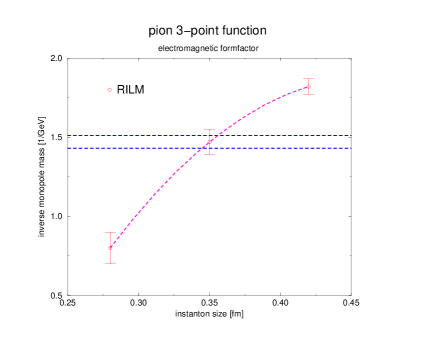
Figure 2: The fitted parameter M of the pion form-factor $ff\sim M^{2}/(Q^{2}+M^{2})$ versus the inputed instanton size.

If so, the following qualitative picture of the QCD vacuum have emerged:

1. Since the instanton size is significantly smaller than the typical separation $R$ between instantons, $\rho/R\sim 1/3$, the vacuum is fairly dilute. The fraction of spacetime occupied by strong fields is only a few percent.

2. The fields inside the instanton are very strong, $G_{\mu\nu}\gg\Lambda_{QCD}^{2}$. This means that the semi-classical approximation is valid, and the typical action is large

   $$S_{0}=8\pi^{2}/g^{2}(\rho)\sim 10-15\gg 1.$$ (27)

   Higher order corrections are proportional to $1/S_{0}$ and presumably small.

3. Instantons retain their individuality and are not destroyed by interactions. From the dipole formula, one can estimate

   $$|\delta S_{int}|\sim(2-3)\ll S_{0}.$$ (28)

4. Nevertheless, interactions are important for the structure of the instanton ensemble, since

   $$\exp|\delta S_{int}|\sim 20\gg 1.$$ (29)

   This implies that interactions have a significant effect on correlations among instantons, and the instanton ensemble in QCD is not a dilute gas but an interacting liquid.

The aspects of the QCD vacuum for which instantons are most important are those related to light fermions. Their importance in the context of chiral symmetry breaking is related to the fact that the Dirac operator has a chiral zero mode in the field of an instanton. These zero modes are localized quark states around instantons, like atomic states of electrons around nuclei. At finite density of instantons those states can become collective, like atomic states in metals. The resulting de-localized state corresponds to the wave function of the quark condensate.

Direct tests of all these ideas on the lattice are possible. One may have a look at the lowest eigenmodes and see if they are related to instantons or something else (monopoles, vortices…) by identifying their shapes - 4d bumps (lines or 2-d sheets) respectively. So far, only bumps (that is the instantons) were seen.

One may also test how locally chiral are the lowest eigenmodes. Just at this school I learned from one of its young participants, Christof Gattringer, about his version of chiral lattice fermions and nice results he got. Among those is remarkably well defined separation between instanton-based and perturbative-like lowest modes, revealed by the so called participation ratios.

Let me now explain about the lowest QCD scale generated by instantons, mentioned above. The width of the zero mode zone of states is of the order of root-mean-square matrix element of the Dirac operator $<I|/D|J>\sim\rho^{2}/R^{3}$. Here states I,J are some instanton and anti-instanton zero modes, rho is the instanton size and $R\sim n^{-1/4}\approx 1fm$ is the distance between their centers. Note small factor $(\rho/R)^{2}\sim 1/10$ here. The Dirac eigenvalues from the zone have similar magnitude. Now, the eigenvalues enter together with quark mass m: and so only when this quark mass is smaller than this scale we start seeing the physics of the zero mode zone. In particular, for quenched QCD (or instanton liquid) there is no determinant and the zone states have rather wrong spectrum. However, only if the quark mass is small compared to its width we start observing the difference. Only recently lattice practitioners were able to do so: indeed, quenched QCD results at small m start deviating from the correct answers quite drastically.

2.7 Interacting instantons

In the QCD partition function there are two types of fields, gluons and quarks, and so the first question one addresses is which integral to take first.

(i) One way is to eliminate $gluonic$ degrees of freedom first. Physical motivation for this may be that gluonic states are heavy and an effective fermionic theory should be better suited to derive an effective low-energy fermionic theory. It is a well-trodden path and one can follow it to the development of a similar four-fermion theory, the NJL model. One can do simple mean field or random field approximation (RPA) diagrams, and find the mean condensate and properties of the Goldstone mesonsDP_86 . The results for Color Super-conductors at high density reported below are done with the same technique as well. But nevertheless, not much can really be done in such NJL-like approach. In fact, multiple attacks during the last 40 years at the NJL model beyond the mean field basically failed. In particular, one might think that since baryons are states with three quarks, and one may wonder if using quasi-local four-fermion Lagrangians for the three body problem is a solvable quantum mechanical problem, and one can at least tell if nucleons are or are not bound in NJL. In fact it is not: the results depend strongly on subtleties of how the local limit for the interaction is defined, and there is no clear answer to this question. Other notorious attempts to sum more complicated diagrams deal with the possible modification of the the chiral condensate. Some works even claim that those diagrams destroy it $completely$!

Going from NJL to instantons improves the situation enormously: the shape of the form-factor is no longer a guess (it is provided by the shape of zero modes) and one can in principle evaluate any particular diagram. However summing them all up still seems like an impossible task.

(ii) The solution to this problem was found. For that one has to follow the opposite strategy and do the $fermion$ integral first. The first step is simple and standard: fermions only enter quadratically, leading to a fermionic determinant. In the instanton approximation, it leads to the Interacting Instanton Liquid Model, defined by the following partition function:

$$Z=\sum_{N_{+},\,N_{-}}{1\over N_{+}!N_{-}!}\int\prod_{i}^{N_{+}+N_{-}}[d\Omega_{i}\;d(\rho_{i})]\exp(-S_{\rm int})\prod_{f}^{N_{f}}\det(\hat{D}+m_{f})\,,$$ (30)

describing a system of pseudo-particles interacting via the bosonic action and the fermionic determinant. Here $d\Omega_{i}=dU_{i}\,d^{4}z_{i}\,d\rho_{i}$ is the measure in color orientation, position and size associated with single instantons, and $d(\rho)$ is the single instanton density $d(\rho)=dn_{I,\bar{I}}/d\rho dz$.

The gauge interaction between instantons is approximated by a sum of pure two-body interaction $S_{\rm int}=\frac{1}{2}\sum_{I\neq J}S_{\rm int}(\Omega_{IJ})$. Genuine three body effects in the instanton interaction are not important as long as the ensemble is reasonably dilute. Implementation of this part of the interaction (quenched simulation) is quite analogous to usual statistical ensembles made of atoms.

As already mentioned, quark exchanges between instantons are included in the fermionic determinant. Finding a diagonal set of fermionic eigenstates of the Dirac operator is similar to what people are doing, e.g., in quantum chemistry when electron states for molecules are calculated. The difficulty of our problem is however much higher, because this set of fermionic states should be determined for $all$ configurations which appear during the Monte-Carlo process.

If the set of fermionic states is however limited to the subspace of instanton zero modes, the problem becomes tractable numerically. Typical calculations in the IILM involved up to N$\sim 100$ instantons (+anti-instantons): which means that the determinants of $N\times N$ matrices are involved. Such determinants can be evaluated by an ordinary workstation (and even PC these days) so quickly that a straightforward Monte Carlo simulation of the IILM is possible in a matter of minutes. On the other hand, expanding the determinant in a sum of products of matrix elements, one can easily identify the sum of all closed loop diagrams up to order $N$ in the ’t Hooft interaction. Thus, in this way one can actually take care of about 100 factorial diagrams!

3 Hadronic Structure and the QCD correlation functions.

3.1 Correlators as a bridge between hadronic and partonic worlds

Consider two currents separated by a $space-like$ distance $x$ (which can be considered as the spatial distance, or an Euclidean time) and introduce correlation functions of the type

$$K(x)=<T(J(x)J(0))>$$ (31)

with $J(x)=\bar{\psi}(x)\Gamma\psi(x)$. The matrix $\Gamma$ contains $\gamma_{\mu}$ for vector currents, $\gamma_{5}$ for the pseudoscalar or $1$ for the scalars, etc, and also a flavor matrix, if needed.

We will start with isovector vector and axial currents, and then discuss 4 scalar-pseudoscalar channels: $\pi$ (P=-1, I=1), $\sigma$ or $f_{0}$ (P=+1,I=0), $\eta$ (P=-1,I=0) and $\delta$ or $a_{0}$ (P=+1,I=1).

In a (relativistic) field theory, correlation functions of gauge invariant local operators are the proper tool to study the spectrum of the theory. The correlation functions can be calculated either from the physical states (mesons, baryons, glueballs) or in terms of the fundamental fields (quarks and gluons) of the theory. In the latter case, we have a variety of techniques at our disposal, ranging from perturbative QCD, the operator product expansion (OPE), to models of QCD and lattice simulations. For this reason, correlation functions provide a bridge between hadronic phenomenology on the one side and the underlying structure of the QCD vacuum on the other side.

Loosely speaking, hadronic correlation functions play the same role for understanding the forces between quarks as the $NN$ scattering phase shifts did in the case of nuclear forces. In the case of quarks, however, confinement implies that we cannot define scattering amplitudes in the usual way. Instead, one has to focus on the behavior of gauge invariant correlation functions at short and intermediate distance scales. The available theoretical and phenomenological information about these functions was recently reviewed in Shu_93 .

In all cases at small x we expect $K(x)\approx K_{0}(x)$ where the latter corresponds to just $free$ propagation of (about massless) light quarks. The zeroth order correlators are all just $K_{0}(x)=12/(\pi^{4}x^{6})$, basically the square of the massless quark propagator.

The first deviations due to non-perturbative effects can be studied using Wilsonian Operator Product Expansion (OPE) in refSVZ . For all scalar and pseudoscalar channels the resulting first correction is

$${K(x)\over K_{0}(x)}=1+{x^{4}\over 384}<(gG)^{2}>+...$$ (32)

The “gluon condensate” is assumed to be made out of a soft vacuum field, and therefore all arguments can be simply taken at the point $x=0$. The so-called $standard$ value of the “gluon condensate” appearing here was estimated previously from charmonium sum rules:

$$<(gG)^{2}>_{SVZ}\approx.5\,GeV^{4}$$ (33)

Thus, the OPE suggests the following scale, at which the correction becomes equal to the first term:

$$x_{OPE}=(384/<(gG)^{2}>_{SVZ})^{1/4}\approx 1.0\,\,fm$$ (34)

This seems to be completely consistent with the approximation used. However, as Novikov, Shifman, Vainshtein and Zakharov soon noticedNSVZ , this (and other OPE corrections) completely failed to describe all the $J^{P}=O^{\pm}$ channels: we return to this issue after we consider vectors and axials.

3.2 Vector and axial correlators

The information available on vector correlation functions from experimental data on $e^{+}e^{-}->hadrons$, the OPE and other exact results was reviewed in Shu_93 . Since then, however, new high statistics measurement of hadronic $\tau$ decays $\tau\rightarrow\nu_{\tau}+{\rm hadrons}$ have been done. For definiteness, we use results of one of them, ALEPH experiment at CERN aleph1 ; aleph2 .

The vector and axial-vector correlation functions are $\Pi_{V}(x)=\langle j^{a}_{\mu}(x)j^{a}_{\mu}(0)\rangle$ and $\Pi_{A}(x)=\langle j^{5\,a}_{\mu}(x)j^{5\,a}_{\mu}(0)\rangle$. Here, $j^{a}_{\mu}(x)=\bar{q}\gamma_{\mu}\frac{\tau^{a}}{2}q$, $j^{5\,a}_{\mu}(x)=\bar{q}\gamma_{\mu}\gamma_{5}\frac{\tau^{a}}{2}q$ are the isotriplet vector and axial-vector currents. The Euclidean correlation functions have the spectral representation Shu_93

$$\Pi_{V,A}(x)=\int ds\,\rho_{V,A}(s)D(\sqrt{s},x),$$ (35)

where $D(m,x)=m/(4\pi^{2}x)K_{1}(mx)$ is the Euclidean coordinate space propagator of a scalar particle with mass $m$. We shall focus on the linear combinations $\Pi_{V}+\Pi_{A}$ and $\Pi_{V}-\Pi_{A}$. These combinations allows for a clearer separation of different non-perturbative effects. The corresponding spectral functions $\rho_{V}\pm\rho_{A}$ measured by the ALEPH collaboration are shown in Fig. 3. The errors are a combination of statistical and systematic ones (below we use them conservatively, as pure systematic): the main problem seems to be separation into V and A of channels with Kaons, which may affect $V-A$ at $s>2\,GeV$ at 10% level. None of our conclusions are sensitive to it.

In QCD, the vector and axial-vector spectral functions must satisfy chiral sum rules. Assuming that $\rho_{V}-\rho_{A}=0$ at above $s>m^{2}_{\tau}$, and using ALEPH data below it, one finds that all 4 of the sum rules are satisfied within the experimental uncertainty, but the central values differ significantly from the chiral predictions aleph1 . In general, both functions are expected to have oscillations of decreasing amplitude, and putting $\rho_{V}-\rho_{A}$ to zero at arbitrary point imply appearance of spurious dimension $d=2,4$ operators in the correlation functions at small x. Therefore, we have decided to terminate the data above a specially tuned point, $s_{0}=2.5\,{\rm GeV}^{2}$, enforcing all 4 chiral sum rules. (The reader should however be aware of the fact that we have, in effect, slightly moved the data points in the small $x$ region within the error band.) Finally we add the pion pole contribution (not shown in Fig. 3), which corresponds to an extra term $\Pi_{A}^{\pi}(x)=f_{\pi}^{2}m_{\pi}^{2}D(m_{\pi},x)$. The resulting correlation functions $\Pi_{V}(x)\pm\Pi_{A}(x)$ are shown in Figs. 4.

We begin our analysis with the combination $\Pi_{V}-\Pi_{A}$. This combination is sensitive to chiral symmetry breaking, while perturbative diagrams, as well as gluonic operators cancel out.

Figure 3: Spectral functions $v(s)\pm a(s)=4\pi^{2}(\rho_{V}(s)+\rho_{A}(s))$ extracted by the ALEPH collaboration from $tau$ lepton hadronic decays.

In Fig. 4 we compare the measured correlation functions with predictions from the instanton liquid model (in its simplest form, random instanton liquid with parameters n, $\rho$ fixed in Shu_82 and discussed above).

The agreement of the instanton prediction with the measured $V-A$ correlation is impressive: it extends all the way from short to large distances. At distances $x>1.25$ fm both combinations are dominated by the pion contribution while at intermediate $x$ the $\rho,\rho^{\prime}$ and $a_{1}$ resonances contribute.

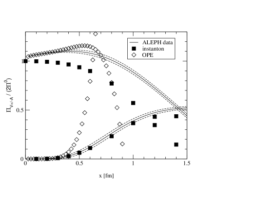
Figure 4: Euclidean coordinate space correlation functions $\Pi_{V}(x)\pm\Pi_{A}(x)$ normalized to free field behavior. The solid lines show the correlation functions reconstructed from the ALEPH spectral functions and the dotted lines are the corresponding error band. The squares show the result of a random instanton liquid model and the diamonds the OPE fit described in the text.

We shall now focus our attention on the $V+A$ correlation function. The unique feature of this function is the fact that the correlator remains close to free field behavior for distances as large as 1 fm. This phenomenon was referred to as “super-duality” in Shu_93 . The instanton model reproduces this feature of the $V+A$ correlator. We also notice that for small $x$ the deviation of the correlator in the instanton model from free field behavior is small compared to the perturbative $O(\alpha_{2}/\pi)$ correction. This opens the possibility of precision studies of the pQCD contribution. But before we do so, let us compare the correlation functions to the OPE prediction

$$\frac{\Pi_{V}(x)+\Pi_{A}(x)}{2\Pi_{0}(x)} = 1+\frac{\alpha_{s}}{\pi}-\frac{1}{384}\langle g^{2}G_{\mu\nu}^{2}\rangle x^{4}$$ (37)

$$\hskip 14.22636pt-\frac{4\pi^{3}}{81}\alpha_{s}(x)\langle{\bar{q}q}\rangle\log(x^{2})x^{6}+\ldots$$

Note that the perturbative correction is attractive, while the power corrections of dimension $d=4$ and $d=6$ are repulsive. Direct instantons also induce an $O(x^{4})$ correction $1-\frac{\pi^{2}}{12}\left(\frac{N}{V}\right)x^{4}+\ldots$ , which is consistent with the OPE because in a dilute instanton liquid we have $\langle g^{2}G^{2}\rangle=32\pi^{2}(N/V)$. This term can indeed be seen in the instanton calculation and causes the correlator to drop below 1 at small $x$. It is possible to extract the value of $\Lambda_{QCD}$ (we find $\alpha_{s}(m_{\tau})=0.35$) and even clear indication of running coupling. It is only possible to do because the non-perturbative corrections (represented by instantons) are basically cancelling each other to very high degree, in V+A channel.

Why is it happening? The first order in ’t Hooft is indeed absent, due to chirality mismatch. There is no general theoretical reason why all non-perturbative of higher order should also do so: but ALEPH data used wrongly hint that they actually do so.

3.3 Spin-zero correlation functions

Now we will see case4s which are completely opposite to those just considered: the instanton-induced effects would be large. Furthermore, the 4 channels actually show completely different non-perturbative deviation from $K_{0}$ at small x: half of them ($\pi,\sigma$) deviate upward, and another pair ($\eta,\delta$) deviate downward.

But let me first demonstrate that the OPE scale determined above cannot be right. All we have to do is to evaluate the strength of the pion contribution to the correlator in question:

$$K_{\pi}(x)={\lambda_{\pi}^{2}\over 4\pi^{2}x^{2}}$$ (38)

The coupling constant is defined as $\lambda_{\pi}=<0|J(0)|\pi>$ and the rest is nothing more than the scalar massless propagator. Because both the pion term and the gluon condensate correction happen to be $1/x^{2}$, let us compare the coefficients. Ideal matching would mean they are about the same

$$\lambda_{\pi}^{2}\approx{<(gG)^{2}>_{SVZ}\over 8\pi^{2}}$$ (39)

The r.h.s. is about 0.0063 GeV⁴. However, phenomenology tells us that (unlike the better known coupling to the axial current $f_{\pi}$) the coupling $\lambda_{\pi}$ is surprisingly large. The l.h.s. of this relation is actually $\lambda_{\pi}^{2}=(.48\,GeV)^{4}=0.053\,GeV^{4}$, about 10 times larger than the r.h.s. It means much larger non-perturbative effect is needed to explain the deviation from the perturbative behavior.

Now, let us see why is it so. The instanton effects in spin-0 channels are in these cases much larger because effect of ’t Hooft interaction appears in those cases in the first order. Furthermore, since it its flavor structure is non-diagonal $(\bar{u}u)(\bar{d}d)$ the correlator of two $\pi^{0}$ currents $(\bar{u}\gamma_{5}u-\bar{d}\gamma_{5}d)$ have it with opposite sign as compared to the correlator of $\eta^{\prime}$ currents $(\bar{u}\gamma_{5}u+\bar{d}\gamma_{5}d)$. What it means is that instantons are as attractive in the pion channel as they are repulsive in the $\eta^{\prime}$ case. The situation is reversed in the scalar channels: the isoscalar sigma is attractive and isovector is repulsive.

Figure 5: Pion correlation function in various approximations and instanton ensembles. In the top figure we show the phenomenological expectation (solid), the OPE (dashed), the single instanton (dash-dotted) and mean field approximations (dashed) as well as data in the random instanton ensemble. In the bottom figure we compare different instanton ensembles, random (open squares), quenched (circles) and interacting (streamline: solid squares, ratio ansatz solid triangles).

Full results from versions of the instanton liquid model for pion correlators are shown in fig.5. Different versions of the model (mentioned in figures below as IILM(rat) etc) differ by a particular ansatz for the gauge field used, from which the interaction is calculated. Note also, that these figures contain also a curve marked “phen”: this is what the correlator actually looks like, according to phenomenology.

We simply show a few results of correlation functions in the different instanton ensembles (see original refs inSS_98 ). Some of them (like vector and axial-vector ones) turned out to be easy: nearly any variant of the instanton model can reproduce the (experimentally known!) correlators well. Some of them are sensitive to details of the model very much: two such cases are shown in Figs. 5-6. The pion correlation functions in the different ensembles are qualitatively very similar. The differences are mostly due to different values of the quark condensate (and the physical quark mass) in the different ensembles. Using the Gell-Mann-Oaks-Renner relation, one can extrapolate the pion mass to the physical value of the quark masses. The results are consistent with the experimental value in the streamline ensemble (both quenched and unquenched), but clearly too small in the ratio ansatz ensemble. This is a reflection of the fact that the ratio ansatz ensemble is not sufficiently dilute.

Figure 6: Eta prime meson correlation functions. The various curves and data sets are labeled as in Fig. 5. Note that random instanton liquid model (RILM) and quenched version (no fermionic determinant, only bosonic interactions) predict $\eta^{\prime}$ correlator to go negative. The same unphysical behavior has been found on the lattice.

The situation is drastically different in the $\eta^{\prime}$ channel. Among the $\sim 40$ correlation functions calculated in the random ensemble, only the $\eta^{\prime}$ and the isovector-scalar $\delta$ were found to be completely unacceptable. The correlation function decreases very rapidly and becomes $negative$ at $x\sim 0.4$ fm. This behavior is incompatible even with a normal spectral representation. The interaction in the random ensemble is too repulsive, and the model “over-explains” the $U(1)_{A}$ anomaly.

The results in the unquenched ensembles (closed and open points) significantly improve the situation. This is related to dynamical correlations between instantons and anti-instantons (topological charge screening). The single instanton contribution is repulsive, but the contribution from pairs is attractive. Only if correlations among instantons and anti-instantons are sufficiently strong are the correlators prevented from becoming negative. Quantitatively, the $\delta$ and $\eta_{\rm ns}$ masses in the streamline ensemble are still too heavy as compared to their experimental values. In the ratio ansatz, on the other hand, the correlation functions even show an enhancement at distances on the order of 1 fm, and the fitted masses are too light. This shows that the $\eta^{\prime}$ channel is very sensitive to the strength of correlations among instantons.

In summary, pion properties are mostly sensitive to global properties of the instanton ensemble, in particular its diluteness. Good phenomenology demands $\bar{\rho}^{4}n\simeq 0.03$, as originally suggested inShu_82 . The properties of the $\rho$ meson are essentially independent of the diluteness, but show sensitivity to $\bar{I}I$ correlations. These correlations become crucial in the $\eta^{\prime}$ channel.

3.4 Baryonic correlation functions

The existence of a strongly attractive interaction in the pseudoscalar quark-antiquark (pion) channel also implies an attractive interaction in the scalar quark-quark (diquark) channel. This interaction is phenomenologically very desirable, because it immediately explains why the nucleon is light, while the delta (S=3/2,I=3/2) is heavy.

The so called Ioffe currents (with no derivatives and the minimum number of quark fields) are local operators which can excite states with nucleon quantum numbers. Those with positive parity and spin $1/2$ can also be represented in terms of scalar and pseudoscalar diquarks

$$\eta_{1,2}=(2,4)\left\{\epsilon_{abc}(u^{a}Cd^{b})\gamma_{5}u^{c}\mp\epsilon_{abc}(u^{a}C\gamma_{5}d^{b})u^{c}\right\}.$$ (40)

Nucleon correlation functions are defined by $\Pi^{N}_{\alpha\beta}(x)=\langle\eta_{\alpha}(0)\bar{\eta}_{\beta}(x)\rangle$, where $\alpha,\beta$ are the Dirac indices of the nucleon currents. In total, there are six different nucleon correlators: the diagonal $\eta_{1}\bar{\eta}_{1},\,\eta_{2}\bar{\eta}_{2}$ and off-diagonal $\eta_{1}\bar{\eta}_{2}$ correlators, each contracted with either the identity or $\gamma\cdot x$. Let us focus on the first two of these correlation functions (for more detail, seeSS_98 and references therein).

Figure 7: Nucleon and delta correlation functions $\Pi_{2}^{N}$ and $\Pi_{2}^{\Delta}$. Curves labeled as in Figs.on mesonic correlators.

The correlation function $\Pi_{2}^{N}$ in the interacting ensemble is shown in Fig. 7. The fact that the nucleon in IILM is actually bound can also be demonstrated by comparing the full nucleon correlation function with that of three non-interacting quarks (the cube of the average propagator). The full correlator is significantly larger than the non-interacting one.

There is a significant enhancement over the perturbative contribution which is nicely described in terms of the nucleon contribution. Numerically, we find $m_{N}=1.019$ GeV. In the random ensemble, we have measured the nucleon mass at smaller quark masses and found $m_{N}=0.96\pm 0.03$ GeV. The nucleon mass is fairly insensitive to the instanton ensemble. However, the strength of the correlation function depends on the instanton ensemble. This is reflected by the value of the nucleon coupling constant, which is smaller in the IILM. InSSV_94 we studied all six nucleon correlation functions. We showed that all correlation functions can be described with the same nucleon mass and coupling constants.

The fitted value of the threshold is $E_{0}\simeq 1.8$ GeV, indicating that there is little strength in the “three quark continuum” (dual to higher resonances in the nucleon channel). A significant part of this interaction was traced down to the strongly attractive scalar diquark channel. The nucleon (at least in IILM) is a strongly bound diquark, plus a loosely bound third quark. The properties of this diquark picture of the nucleon continue to be disputed by phenomenologists. We will return to diquarks in the next section, where they will become Cooper pairs of Color Super-conductors.

In the case of the $\Delta$ resonance, there exists only one independent Ioffe current, given (for the $\Delta^{++}$) by

$$\eta^{\Delta}_{\mu}=\epsilon_{abc}(u^{a}C\gamma_{\mu}u^{b})u^{c}.$$ (41)

However, the spin structure of the correlator $\Pi^{\Delta}_{\mu\nu;\alpha\beta}(x)=\langle\eta^{\Delta}_{\mu\alpha}(0)\bar{\eta}^{\Delta}_{\nu\beta}(x)\rangle$ is much richer. In general, there are ten independent tensor structures, but the Rarita-Schwinger constraint $\gamma^{\mu}\eta_{\mu}^{\Delta}=0$ reduces this number to four.

The mass of the delta resonance is too large in the random model, but closer to experiment in the unquenched ensemble. Note that,similar to the nucleon, part of this discrepancy is due to the value of the current mass. Nevertheless, the delta-nucleon mass splitting in the unquenched ensemble is $m_{\Delta}-m_{N}=409$ MeV, larger but comparable to the experimental value 297 MeV. It mostly comes from the absent scalar diquarks in $\Delta$ channel.

4 The Phases of QCD

4.1 The Phase Diagram

In this section we discuss QCD in extreme conditions, such as finite temperature/density. Let me first emphasize why it is interesting and instructive to do. It is not simply to practice once again the semi-classical or perturbative methods similar to what have been done before in vacuum. What we are looking for here are new phases of QCD (and related theories), namely new self-consistent solutions which differ qualitatively from what we have in the QCD vacuum.

One such phase occurs at high enough temperature $T>T_{c}$: it is known as Quark Gluon Plasma (QGP). It is a phase understandable in terms of basic quark and gluon-like excitationsShu_80 , without confinement and with unbroken chiral symmetry in the massless limit. One of the main goals of heavy ion program, especially at new the dedicated Brookhaven facility RHIC, is to study transitions to this phase.

Another one, which has been getting much attention recently, is the direction of finite density. Very robust Color Superconductivity was found to be the case here. Let me also mention one more frontier which has not yet attracted sufficient attention: namely a transition (or many transitions?) as the number of light flavors $N_{f}$ grows. The minimal scenario includes a transition from the usual hadronic phase to a more unusual QCD phase, the $conformal$ one, in which there are no particle-like excitations and correlators are power-like in the infrared. Even the position of the critical point is unknown. The main driving force of these studies is the intellectual challenge it provides.

The QCD phase diagram as we understand it now is shown in Fig 8(a), in the baryonic chemical potential $\mu$ (normalized per quark, not per baryon) and the temperature T plane. Some part of it is old: it has the hadronic phase at small values of both parameters, and QGP phase at large T,$\mu$.

The phase transition line separating them most probably does not really start at $T=T_{c},\mu=0$ but at an “endpoint” E, a remnant of the so called QCD tricritical point which QCD has in the chiral (all quarks are massless) limit. Although we do not know where it is, we hope to find it one day in experiment. The proposed ideas rotate around the fact that the order parameter, the VEV of the sigma meson, is at this point truly massless, and creates a kind of “critical opalecence”. Similar phenomena were predicted and then indeed observed at the endpoint of another line (called M from multi-fragmentation), separating liquid nuclear matter from the nuclear gas phase.

The large-density (and low-T) region looks rather different from what was shown at conferences just a year ago: two new Color Super-conducting phases appear there. Unfortunately heavy ion collisions do not cross this part of the phase diagrams and so it belongs to neutron star physics.

Figure 8: Schematic phase diagram of QCD, in temperature T- baryon chemical potential $\mu$ plane. E and M show critical endpoints of first order transitions: M (from multi-fragmentation) is that for liquid-gas transition in nuclear matter. The color superconducting phases, CSC2 and CSC3 are explained in the text.

Above I mentioned an approach to high density starting from the vacuum. One can also work out in the opposite direction, starting from very large densities and going down. Since the electric part of one-gluon exchange is screened, and therefore the Cooper pairs appear due to magnetic forces. It is interesting by itself, as a rare example: one has to take care of time delay effects of the interaction. The result is indefinitely growing gaps at large $\mu>10GeV$, as Son $\Delta\sim\mu exp(-{3\pi^{2}\over\sqrt{2}g(\mu)})$.

4.2 Finite Temperature transition and Large Number of Flavors

There is no place here to discuss in detail the rather extensive lattice data available now, and I only mention some results related to instantons. In the vacuum a quasi-random set of instantons leads to chiral symmetry breaking and quasi-zero modes: but what in the same terms does the high-T phase look like?

The simplest solution would be just $suppression$ of instantons at $T>T_{c}$, and at some early time people thought this is what actually happens. However, it should not be like this because the Debye screening which is killing them only appears at $T=T_{c}$. Lattice data works have also found no depletion of the instanton density up to $T=T_{c}$.

On the other hand, the absence of the condensate and quasi-zero modes implies that the “liquid” is now broken into finite pieces. The simplest of them are pairs, or the instanton-anti-instanton molecules. This is precisely what instanton simulations have foundSS_98 , see fig.9. Whether it is indeed so on the lattice is not yet clear: nice molecules were located, but the evidence for the molecular mechanism of chiral restoration is still far from being convincing. (No alternative I am aware of have been so far proposed, though.)

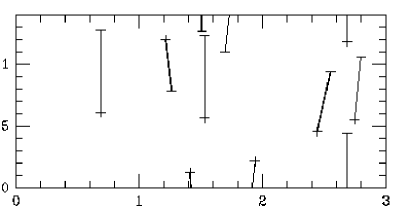
Figure 9: Typical configuration from instanton liquid simulation, at $T>T_{c}$. Lines indicate the direction in which quark propagators are the largest. Clear pairing of instantons and instantons are observed: the pairs tend to have the same spatial position and being separated mostly by Euclidean time.

The results of IILM simulations with variable number of flavors $N_{f}=2,3,5$ flavors with equal masses can be summarized as follows. For $N_{f}=2$ there is a second order phase transition which turns into a line of first order transitions in the $m-T$ plane for $N_{f}>2$. If the system is in the chirally restored phase ($T>T_{c}$) at $m=0$, we find a discontinuity in the chiral order parameter if the mass is increased beyond some critical value. Qualitatively, the reason for this behavior is clear. While increasing the temperature increases the role of correlations caused by fermion determinant, increasing the quark mass has the opposite effect. We also observe that increasing the number of flavors lowers the transition temperature. Again, increasing the number of flavors means that the determinant is raised to a higher power, so fermion induced correlations become stronger. For $N_{f}=5$ we find that the transition temperature drops to zero and the instanton liquid has a chirally symmetric ground state, provided the dynamical quark mass is less than some critical value. Studying the instanton ensemble in more detail shows that in this case, all instantons are bound into molecules.

Unfortunately, little is known about QCD with large numbers of flavors from lattice simulations. There are data by the Columbia group for $N_{f}=4$. The most important result is that chiral symmetry breaking effects were found to be drastically smaller as compared to $N_{f}=0,2$. In particular, the mass splittings between chiral partners such as $\pi-\sigma,\,\rho-a_{1},\,N(\frac{1}{2}^{+})-N(\frac{1}{2}^{-})$, extrapolated to $m=0$ were found to be 4-5 times smaller. This agrees well with what was found in the interacting instanton model: more work in this direction is certainly needed.

4.3 High Density and Color Superconductivity

This topic is covered in detail by Prof.Alford at this school, so I only add few remarks to his lectures.

Although the idea of color superconductivity originates from 70’s, the field of high density QCD was in the dormant state for long time till two papers RSSV ; ARW (posted on the same day) in 1998 have claimed gaps about 100 times larger than previously thought. The field is booming since, as one can see from about 250 citations in 2 years those papers got.

Then-Princeton group (Alford-Rajagopal-Wilczek) have been thinking about different pairings from theory perspective, but our (Stony Brook) team (Rapp,Schafer,ES,Velkovsky) had started from the impressive qq pairing phenomenon found theoretically SSV_94 in the instanton liquid model inside the nucleon. As explained above, we have found it to be, roughly speaking, a small drop of CS matter, made of one Cooper pair of sort (the ud scalar diquark) and one massive quark . T.Schafer heroically attempted numerical simulations of the instanton liquid model at finite $\mu$: although he was not very successful he found out strange “polymers” made of instantons connecting by 2 through going quark lines. It take us some time to realize we see paths of condensed diquarks! It was like finding superconductivity by watching electrons moving on your computer screen.

The main point I would like to emphasize here is that the $qq$ pairing of such diquarks have in fact deep dynamical roots: it follows from the same basic dynamics as the “superconductivity” of the QCD vacuum, the chiral ($\chi$-)symmetry breaking. These spin-isospin-zero diquarks are related to pions, as we will see below.

The most straightforward argument for deeply bound diquarks came from the bi-color ($N_{c}=2$) theory: in it the scalar diquark is degenerate with pions. By continuity from $N_{c}=2$ to $3$, a trace of it should exist in real QCD.

Instantons create the following amusing triality: there are three attractive channels which compete: (i) the instanton-induced attraction in $\bar{q}q$ channel leading to $\chi$-symmetry breaking. (ii) The instanton-induced attraction in $qq$ which leads to color superconductivity. (iii) The light-quark-induced attraction of $\bar{I}I$, which leads to pairing of instantons into “molecules” and a Quark-Gluon Plasma (QGP) phase without $any$ condensates.

At very high density we also can find arbitrarily dilute instanton liquid, as shown recently in SSZ . The reason it cannot exist in vacuum or high T is that if instanton density goes below some critical value, the cannot be any condensate. (The system then breaks into instanton molecules or other clusters and chiral symmetry is restored.) However at high density the superconducting condensate can be created perturbatively as well (we mentioned it above) and there is no problem. The dilute instantons interact by exchanging very light $\eta^{\prime}$ (which would be massless without instantons): one can calculate effective Lagrangian, theta angle dependence etc.

Bi-color QCD: a very special theory One reason it is special (well known to to the lattice community): its fermionic determinant is $real$ even for non-zero $\mu$, which makes simulations possible. However the major interest in this theory is related the so called Pauli-Gursey symmetry. We have argued above that pions and diquarks appear at the same one-instanton level, and are so to say brothers. In bi-color QCD they becomes identical twins: due to the additional symmetry mentioned the diquarks are degenerate with mesons.

In particular, chiral symmetry breaking is done like this $SU(2N_{f})\rightarrow Sp(2N_{f})$, and for $N_{f}=2$ the coset $K=SU(4)/Sp(4)=SO(6)/SO(5)=S^{5}$. Those 5 massless modes are pions plus the scalar diquark $S$ and its anti-particle $\bar{S}$.

Vector diquarks are degenerate with vector mesons, etc. Therefore, the scalar-vector splitting is in this case about twice the constituent quark mass, or about 800 MeV. It should be compared to binding in the “real” $N_{c}=3$ QCD of only 200-300 MeV, and to zero binding in the large-$N_{c}$ limit.

The corresponding sigma model describing this $\chi$-symmetry breaking was worked out inRSSV : for further development seeKST . As argued in RSSV , in this theory the critical value of the transition to Color Superconductivity is simply $\mu=m_{\pi}/2$, or zero in the chiral limit. The diquark condensate is just a rotated $<\bar{q}q>$ one, and the gap is the constituent quark mass. Recent lattice works 2col display it in great detail, building confidence for other cases.

New studies reveal possible new crystalline phases. These phases still have somewhat debatable status, so I have not indicated them on the phase diagram.

Once again, there were two papers submitted by chance on the same day. The “Stony Brook” teamRSZ have found that a “chiral crystal” with oscillating $<\bar{q}q(x)>$ (similar to Overhouser spin waves in solid state) can compete with the BCS 2-flavor superconductor at its onset, or $\mu\approx 400\,MeV$. The proper position of this phase is somewhere in between the hadronic phase (with constant $<\bar{q}q>$) and color superconductor.

The “MIT group”ABR have looked at the oscillating superconducting condensate $<qq(x)>$, following earlier works on the so called LOFF phase in usual superconductors. They have found that it is appearing when the difference between Fermi momenta of different quark flavors become comparable to the gap. The natural place for it on the phase diagram is close to the line at which color superconductivity disappears because the gap goes to zero.

5 High Energy Collisions of hadrons and Heavy Ions

5.1 The Little Bang: AGS, SPS and now the RHIC era

Let me start with brief comparison of these two magnificent explosions: the Big Bang versus the Little Bang, as we call heavy ion collisions.

The expansion law is roughly the Hubble law in both, $v(r)\sim r$ although strongly anisotropic in the Little Bang. The Hubble constant tells us the expansion rate today: similarly radial flow tells us the final magnitude of the transverse velocity. The acceleration history is not really well measured. For Big Bang people use distance supernovae, we use $\Omega^{-}$ which does not participate at the late stages to learn what was the velocity earlier. Both show small dipole (quadrupole or elliptic for Little Bang) components which has some physics, and who knows maybe we will see higher harmonics fluctuations later on, like in Universe. As we will discuss below, in both cases the major puzzle is how this large entropy has been actually produced, and why it happened so early.

The major lessons we learned from AGS experiments ($E_{LAB}=2-12AGeV$) are:
(i) Strangeness enhancement over simple multiple NN collisions appear from very low energies, and heavy ion collisions quickly approach nearly ideal chemical equilibrium of strangeness.
(ii) “Flows” of different species, in their radial,directed and elliptical form, are in this energy domain driven by collective potentials and absorptions: they are not really flows in hydro sense. All of them strongly diminish by the high end of the AGS region, demonstrating the onset of “softness” of the EoS. Probably it is some precursor of the QCD phase transition.

Several important lessons came so far from CERN SPS data:
(i) Much more particle ratios have been measured there: overall those show surprisingly good degree of chemical equilibration: the chemical freeze-out parameters are tantalizingly close to the QGP phase boundary.
(ii) Dileptons show that radiation spectral density is very different in dense matter compared to ideal hadronic gas. The most intriguing data are CERES finding of “melting of the $\rho$”, which seem to be transformed into a wide continuum reaching down to invariant masses as low as 400 MeV. It puts in doubt “resonance gas” view of hadronic matter at these conditions. Intermediate mass dileptons studied by NA50 can be well described by thermal radiation with QGP rates.
(iii)The impact parameter of $J/\psi$ and $\psi^{\prime}$ suppression in PbPb collisions studied by NA50 collaboration shows rather non-trivial behavior. More studies are needed, including especially measurements of the open charm yields, to understand the origin and magnitude of the suppression.

However, during last several months those discussions have been overshadowed by a list of news from RHIC, Relativistic Heavy Ion Collider at Brookhaven National Laboratory. It had its first run in summer 2000 and reported recently at Quark Matter 2001 conference QM01 : many details are discussed in Prof.M.Gylassy’s lectures.

A brief summary is as follows. These results have shown that heavy ions collisions (AA) at these energies significantly differ $both$ from the pp collisions at high energies and the AA collisions at lower (SPS/AGS) energies. The main features of these data are quite consistent with the Quark-Gluon Plasma (QGP) (or Little Bang) scenario, in which entropy is produced promptly and subsequent expansion is close to adiabatic expansion of equilibrated hot medium.

(Let me mention here two other pictures of the heavy ion production, discuss prior to appearance of these data. One is the string picture, used in event generators like RQMD and UrQMD: they predicted effectively very soft EoS and elliptic flow decreasing with energy. The other one is pure minijet scenario, in which most secondaries would come from independently fragmenting minijets. If so, there are basically no collective phenomena whatsoever.)

Already the very first multiplicity measurements reported by PHOBOS collaboration PHOBOS have shown that particle production per participant nucleon is no longer constant, as was the case at lower (SPS/AGS) energies. This new component may be due to long-anticipated pQCD processes, leading to perturbative production of new partons. Unlike high $p_{t}$ processes resulting in visible jets, those must be undetectable “mini-jets” with momenta $\sim 1-2\,GeV$. Production and decay of such mini-jets was discussed in Refs minijets , also this scenario is the basis of widely used event generator HIJING HIJING . Its crucial parameter is the cutoff scale $p_{min}$: if fitted from pp data to be 1.5-2 $GeV$, it leads to predicted mini-jet multiplicity $dN_{g}/dy\sim 200$ for central AuAu collisions at $\sqrt{(}s)=130\,AGeV$. If those fragment independently into hadrons, and are supplemented by “soft” string-decay component, the predicted total multiplicity was found to be in good agreement with the first RHIC multiplicity data. Because partons interact perturbatively, with their scattering and radiation being strongly peaked at small angles, their equilibration is expected to be relatively long equilibr . However, new set of RHIC data reported in QM01 have provided serious arguments against the mini-jet scenario, and point toward quite rapid entropy production rate and early QGP formation.

(i) If most of mini-jets fragment independently, there is no collective phenomena such as transverse flow related with the QGP pressure. However, it was found that those effects are very strong at RHIC. Furthermore, STAR collaboration have observed very robust elliptic flow STAR , which is in perfect agreement with predictions of hydrodynamical model h2hflow ; Kolb assuming equilibrated QGP with its full pressure $p\approx\epsilon/3$ above the QCD phase transition. This agreement persists to rather peripheral collisions, in which the overlap almond-shaped region of two nuclei is only a couple fm thick. STAR and PHENIX data on spectra of identified particles, especially $p,\bar{p}$, indicate spectacular radial expansion, also in agreement with hydro calculations h2hflow ; Kolb . (ii) Spectra of hadrons at large $p_{t}$, especially the $\pi^{0}$ spectra agree well with HIJING for peripheral collisions, but show much smaller yields for central ones, with rather different, (exponential-shaped) spectra. It means long-anticipated “jet quenching” at large $p_{t}$ is seen for the first time, with a surprisingly large suppression factor $\sim 1/5$. Keeping in mind that jets originating from the surface outward cannot be quenched, the effect seem to be as large as it can possibly be. For that to happen, the outgoing high-$p_{t}$ jets should propagate through matter with parton population larger than the abovementioned minijet density predicted by HIJING.

(iii) Curious interplay between collective and jet effects have also been studied by STAR collaboration, in form of elliptic asymmetry parameter $v_{2}(p_{t})$. At large transverse momenta $p_{t}>2\,GeV$ the data depart from hydro predictions and levels off. When compared to predictions of jet quenching models worked out in GVW , they also indicate gluon multiplicity several times larger than HIJING prediction, and are even consistent with its maximal possible value evaluated from the final entropy at freeze-out, $(dN/dy)_{\pi}\sim 1000$.

5.2 Collective flows and EoS

If we indeed have produced excited matter (rather than just a bunch of partons which fly away and fragment independently), we expect to see certain collective phenomena. Ideally, those should be quantitatively reproduced by relativistic hydrodynamics which is basically just local energy-momentum conservation plus the EoS we know from the lattice and models.

The role of the QCD phase transition in matter expansion is significant. QCD lattice simulations lattice show approximately 1st order transition. Over a wide range of energy densities $e=.5-1.4\,GeV/fm^{3}$ the temperature T and pressure p are nearly constant. So the ratio of pressure to energy density, $p/e$, decreases till a minimum at particular energy density $e_{sp}\approx 1.4\,GeV/fm^{3}$, known as the softest point HS-freeze . Near $e_{sp}$ small pressure gradient can not effectively accelerate the matter and the evolution stagnates. However when the initial energy density is well above the QCD phase transition region, $p/e\approx 1/3$, and this pressure drives the collective motion. The energy densities reached at time $\sim 1fm/c$ at SPS($\sqrt{s}_{NN}=17\,GeV$) and RHIC ($\sqrt{s}_{NN}=130\,GeV$) are about 4 and 8 $GeV/fm^{3}$, respectively. We found that at RHIC conditions we are in the latter regime, and matter accelerates to $v\sim.2c$ $before$ entering the soft domain. Therefore by freeze-out this motion changes the spatial distribution of matter dramatically: e.g. as shown in TS_nut the initial almond-shape distribution 10 fm/c later looks like two separated shells, with a little “nut” in between.

The simplest way to see hydro expansion is in spectra of particles: on top of chaotic thermal distributions $\sim exp(-m_{t}/T),m_{t}^{2}=p_{t}^{2}+m^{2}$ one expect to see additional broadening due to hydro outward motion. This effect is especially large if particles are heavy, since flow with velocity v add momentum $mv$.

Derek Teaney h2hflow have developed a comprehensive Hydro-to-Hadrons (H2H) model combines the hydrodynamical description of the initial QGP/mixed phase ($e>.5GeV/fm^{3}$) stages, where hadrons are not appropriate degrees of freedom, with a hadronic cascade RQMD for the hadronic stage. In this way, we can include different EoS displaying properties of the phase transition, and also incorporate complicated final state interaction at freeze-out. The set of EoS used is shown in Fig.10.

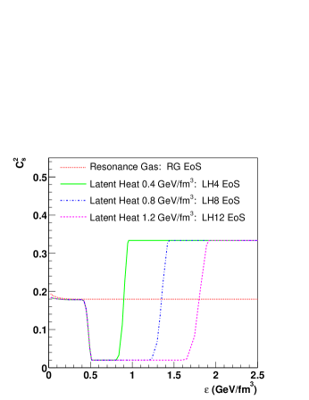
Figure 10: The EoSs in form squared speed of sound $c^{2}=dp/d\epsilon$ with variable Latent Heats $.4GeV/fm^{3}$, $.8GeV/fm^{3}$,.. labeled as LH4, LH8,..versus the energy density.

Radial flow is usually characterized by the slope parameter T: each particle spectra are fitted to the form $dN/dp_{t}^{2}dy\sim exp(-m_{t}/T),m_{t}^{2}=p_{t}^{2}+m^{2}$.Although we denoted the slope by T, it is $not$ the temperature: it incorporates random thermal motion and collective transverse velocity. The SPS NA49 slope parameters for pion and protons are shown in Fig. 11(a). Parameter T grows with particle multiplicity due to increased velocity of the radial flow. Furthermore, the rate of growth depends on the EoS: the softer it is, the less growth. The SPS NA49 data correspond to two data points (our fits to spectra) favor the (relatively stiff) LH8 EoS. (Details of the fit, discussion of the b-dependence etc see in h2hflow .) It is very important to get these parameters for RHIC, especially for heavy secondaries like nucleons and hyperons.

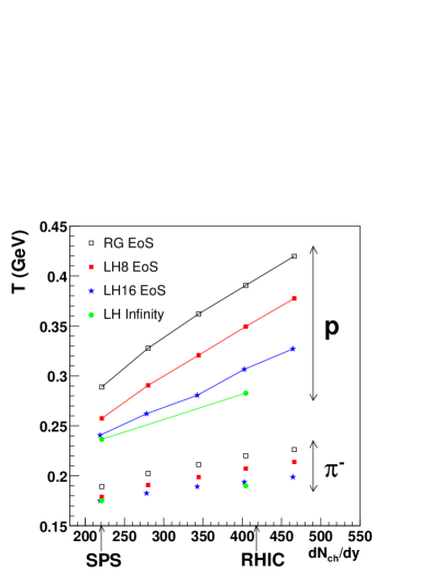
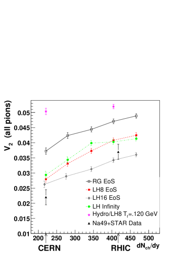
Figure 11: The transverse mass slope T (a) and elliptic flow parameter $V_{2}$ (b) versus midrapidity (y=0) charged purticle multiplicity, for AuAu collisions with b=6.

For $non-central$ collisions the overlap region in the transverse plane has an elliptic, “almond”, shape, and larger pressure gradient force matter to expands preferentially in the direction of the impact parameter Ollitrault . Compared to radial flow, the elliptic flow is formed earlier, and therefore it measures the early pressure. The elliptic flow is quantified experimentally by measuring the azimuthal distributions of the produced particles and calculating the elliptic flow parameter $V_{2}=\langle cos(2\phi)\rangle$ where $\phi$ angle is measured with respect to the impact parameter direction, around the beam axis. It appears due to the elliptic $spatial$ deformation of the overlap region in the nucleus-nucleus collision, quantified by its eccentricity $\epsilon_{2}=<y^{2}-x^{2}>/<x^{2}+y^{2}>$, usually calculated in Glauber model. Since the effect ( $v_{2}$) is proportional to the cause ($\epsilon_{2}$), the ratio $v_{2}/\epsilon_{2}$ does not have strong dependence on the impact parameters b, and this ratio is often used for comparison. (We would not do that below, in the detailed comparison to data, because $\epsilon_{2}(b)$ is not directly measured.

In figure 11(b) the elliptic flow of the system is plotted as a function of charged particle multiplicity at an impact parameter of 6 fm. Before discussing the energy dependence, let us quantify the magnitude of elliptic flow at the SPS. Ideal relativistic hydrodynamics used in earlier works Ollitrault ; Kolb generally over-predicts elliptic flow by about factor 2. Example of such kind is indicated by a star in figure 11(b): it is our hydro result (with LH8 EoS) which has been followed hydrodinamically till very late stages, the freeze-out temperature $T_{f}=120\,MeV$. By switching to hadronic cascade at late stages, we have more appropriate treatment of resonance decays and re-scattering rate, and so one can see that it significantly reduces $V_{2}$, to the range much closer to the data points.

One might thing that one can also do that by simply taking softer EoS, e.g. increasing the latent heat. However, it only happens till LH16 and then $v_{2}$ start even slightly increase again. The explanation of this non-monotonous behavior is the interplay of the initial “QGP push” for stiffer EoS, with longer time for hadronic stage available for softer EoS. We cannot show here details, but it turns out that a given (experimental) $V_{2}$ value can correspond to two different solutions, one with earlier push and another with the later expansion dominating. Coincidentally, STAR data point happen to be right at the onset of such a bifurcation, close to LH16. The multiplicity dependence of $V_{2}$ appears simple from figure LABEL:pspionV2dNdy(b): all curve show growth with about the same rate. Note however that such growth of $V_{2}$ from SPS to RHIC (first predicted in Shu_QM99 where our first preliminary results has been shown) Is not shared by most other models. In particular, string-based models like UrQMD predicts a decrease by a factor of $\approx 2$ UrQMD_Bleicher . It happens because strings produce no transverse pressure and so the effective EoS is super-soft at high energies. Models based on independent parton scattering and decay (such as HIJING) also predict basically vanishing (or slightly negative)HIJING $V_{2}$.

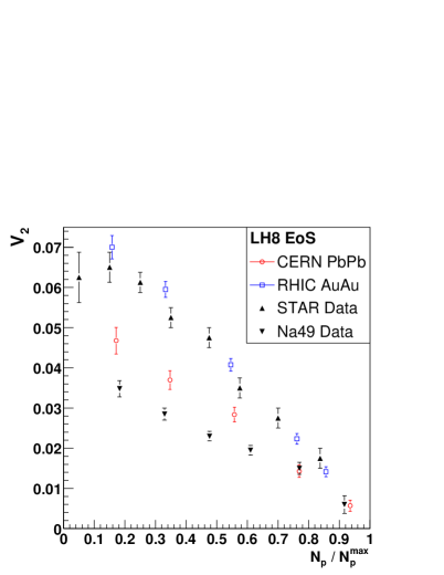
Figure 12: v2 versus impact parameter b, described experimentally by the number of participant nucleons, for RHIC STAR and SPS NA49 experiments. Both are compared to our results, for EoS LH8.

In Fig.12 we show how our results compare with data as a function of impact parameter. One can see that the agreement becomes much better at RHIC. Furthermore, one may notice that deviation from linear dependence we predict becomes visible at SPS for more peripheral collisions with $N_{p}/N_{p}^{max}<0.6$ or so, while at RHIC only the most peripheral point, with $N_{p}/N_{p}^{max}=0.05$ show such deviation. This clearly shows that hydrodynamical regime in general works much better at RHIC.

In summary, the flow phenomena observed at RHIC are stronger than at SPS. It is in complete agreement with the QGP scenario. All data on elliptic and radial flow can be nicely reproduced by the H2H model. Furthermore, we are able to restrict the EoS, to those with the latent heat about .8 $GeV/fm^{3}$.

5.3 How QGP happened to be produced/equilibrated so early?

One possible solution to the puzzle outline above can be a significantly lower cutoff scale in AA collisions, as compared to $p_{min}=1.5-2\,GeV$ fitted from the pp data. That increases perturbative cross sections, both due to smaller momenta transfer and larger coupling constant. As I argued over the years, the QGP is a new phase of QCD which is qualitatively different from the QCD vacuum: therefore the cut-offs of pQCD may have entirely different values and be determined by different phenomena. Furthermore, since QGP is a plasma-like phase which screens itself perturbatively Shu_80 , one may think of a cut-offs to be determined self-consistently from resummation of perturbative effects. These ideas known as self-screening or initial state saturation were discussed in Refs. equilibr . Although the scale in question grows with temperature or density, just above $T_{c}$ it may actually be smaller than the value 1.5-2 GeV we observe in the vacuum. Its first experimental manifestation may be dropping of the so called “duality scale” in the observed dilepton spectrum, see discussion in RW .

Another alternative to explain large gluon population at RHIC would be an existence of more rapid multi-gluon production processes. Let us consider an alternative $non-perturbative$ scenario based entirely on non-perturbative processes involving instantons and sphalerons my_sph . But before we do that, we have to take a look at hadronic collisions and briefly review few recent papers on the subject.

At $s>10^{3}GeV^{2}$ hadronic cross sections as $\bar{p}p,pp,\pi p,Kp$, $\gamma N$ and even $\gamma\gamma$ slowly grow with the collision energy s. This behavior can be well parameterized by soft Pomeron phenomenology, but we will only use its logarithmically growing part

$$\sigma_{hh^{\prime}}(s)=\sigma_{hh^{\prime}}(s_{0})+log(s/s_{0})X_{hh^{\prime}}\Delta+...$$ (42)

ignoring both the higher powers of log(s) and decreasing Regge terms. We will use those two parameters from PDG-2000 recent fits, the intercept and its coefficient in $pp,\bar{p}p$ collisions, $\Delta=\alpha(0)-1=0.093(2),\,X_{NN}=18.951(27)\ mb.$ Note a qualitative difference between constant and logarithmically growing parts of t he cross section. The former can be explained by prompt color $exchanges$, as suggested by Low and Nussinov long ago. It nicely correlates with flux tube picture of the final state. section.) The $growing$ part of the cross section cannot be generated by t-channel color exchanges and is associated with processes promptly producing some objects, with log(s) coming from the longitudinal phase space. In pQCD it is gluon production, by processes like the one shown in Fig.13(a). If iterated in the t-channel in ladder-type fashion, the result is approximately a BFKL pole BFKL . Although the power predicted is much larger than $\Delta$ mentioned, it seem to be consistent with much stronger growth seen in hard processes at HERA: thus it is therefore sometimes called the “hard pomeron”. The physical origin of cross section growth remains an outstanding open problem: neither the perturbative resummations nor many non-perturbative models are really quantitative. It is hardly surprising, since scale at which soft Pomeron operates (as seen e.g. from the Pomeron slope $\alpha^{\prime}(0)\approx 1/(2\,GeV)^{2}$) is also the “substructure scale” mentioned above.

Recent application of the instanton-induced dynamics to this problem have been discussed in several papers pom_inst . Especially relevant for this Letter are two last works which use insights obtained a decade ago in discussion of instanton-induced processes in electroweak theory weakinst , and the growing part of the hh cross sections were ascribed to multi-gluon production via instantons, see Fig.13(b). Among qualitative features of this theory is the explanation of why no odderon appears (instantons are SU(2) objects, in which quarks and antiquarks are not really distinct), an explanation of the small power $\Delta$ (it is proportional to “instanton diluteness parameter” $n\rho^{4}$ mentioned above), the small size of the soft Pomeron (governed simply by small size of instantons $\rho\sim 1/3\,fm$). Although instanton-induced amplitudes contain small “diluteness” factor, there is no extra penalty for production of new gluons: thus one should expect instanton effects to beat perturbative

amplitudes of sufficiently high order. This generic idea is also behind the present work, dealing with prompt multi-gluon production.

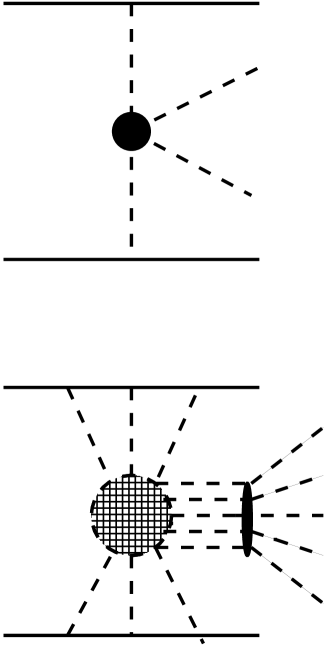
Figure 13: (a) A typical inelastic perturbative process: two t-channel gluons collide, producing a pair of gluons; (b) Instanton-induced inelastic process incorporate collisions of multiple t-channel gluons with the instanton (the shaded circle), resulting in multi-gluon production. The intermediate stage of the process, indicated by the horizontal dashed lines, corresponds to a time when outgoing glue is in the form of coherent field configuration - the $sphaleron$. Since this part of the process corresponds to motion above the barrier, it does not enter the calculation of the cross section, but is only needed for prediction of the inclusive spectra, multiplicities etc.

Technical description of the process can be split into two stages. The first (at which one evaluates the probability) is the motion under the barrier, and it is described by Euclidean paths approximated by instantons. Their interaction with the high energy colliding partons results in some energy deposition and subsequent motion over the barrier. At this second stage the action is real, and the factor $exp(iS)$ does not affect the probability, and we only need to consider it for final state distributions. The relevant Minkowski paths start with configurations close to the QCD analogs of electroweak sphalerons Manton , static spherically symmetric clusters of gluomagnetic field which satisfy the Yang-Mills equations. (Those can be obtained from known electroweak solutions in the limit of infinitely large Higgs self-coupling.) Their mass in QCD is

$$M_{sph}\approx{30\over g^{2}(\rho)\rho}\sim 2.5\,GeV$$ (43)

Since those field configurations are close to classically unstable saddle point at the top of the barrier, they roll downhill and develop gluoelectric fields. When both become weak enough, solution can be decomposed into perturbative gluons. This part of the process can also be studied directly from classical Yang-Mills equation: for electroweak sphalerons it has been done in Refssphaleron_decay , calculation for its QCD version is in progress CS . While rolling, the configurations tend to forget the initial imperfections (such as a non-spherical shapes) since there is only one basic instability path downward: so the resulting fields should be nearly perfect spherical expanding shells. Electroweak sphalerons decay into approximately 51 W,Z,H quanta, of which only about 10% are Higgses, which carry only 4% of energy. Ignoring those, one can estimate mean gluon multiplicity per sphaleron decay, by simple re-scaling of the coupling constants: the result gives 3-4 gluons. Although this number is not large, it is important to keep in mind that they appear as a coherent expanding shell of strong gluonic field.

It has been suggested in my_sph that if sphaleron-type object are copiously produced, with or instead of $p\sim 1GeV$ minijets, they may significantly increase the entropy produced and speed up the equilibration process.

Acknowledgments. It is a pleasure to thank the organizers of the school for their invitation: it was indeed a very interesting and successful one. This work was supported in parts by the US-DOE grant DE-FG-88ER40388.

References

- (1) T. Schafer and E.V. Shuryak. Rev.Mod.Phys.70 323 1998 hep-ph/9610451
- (2) CHIRAL SYMMETRY BREAKING BY INSTANTONS. D.Diakonov, In *Varenna 1995, Selected topics in nonperturbative QCD* 397-432. e-Print Archive: hep-ph/9602375
- (3) E. V. Shuryak. Rev. Mod. Phys. 651 1993
- (4) M.A. Shifman, A.I. Vainshtein, V.I. Zakharov, Phys.Lett.76B 4711978
- (5) E.V. Shuryak. Nucl.Phys.B20393,116,140 1982
- (6) V. A. Novikov, M. A. Shifman, A. I. Vainshtein, and V. I. Zakharov. Nucl. Phys.B191301 1981
- (7) A.A Belavin, A.M. Polyakov, A.S. Schvartz, Yu.S. Tyupkin, Phys.Lett.B59:85-87,1975
- (8) S. L. Adler. Phys. Rev., 177:2426, 1969.
- (9) J. S. Bell and R. Jackiw. Nuo. Cim., A60:47, 1969.
- (10) A. Hasenfratz and C.Nieter, Instanton Content of the SU(3) Vacuum,hep-lat/9806026.
- (11) G. ’t Hooft. Phys. Rev. D14,3432, 1976
- (12) Y. Nambu and G. Jona-Lasinio. Phys. Rev.122345 1961.
- (13) D.Diakonov, V.Yu. Petrov Nucl.Phys.B272:457,1986
- (14) M.A. Shifman, A.I. Vainshtein, V.I. Zakharov, Nucl.Phys.B165:45,1980
- (15) A.Blotz, E.V.Shuryak, Phys.Rev.D55:4055-4065,1997
- (16) R. Barate et al. [ALEPH Collaboration], Z. Phys. C76, 15 (1997).
- (17) R. Barate et al. [ALEPH Collaboration], Eur. Phys. J. C4, 409 (1998).
- (18) T. Schäfer, E. V. Shuryak, and J. J. M. Verbaarschot. Nucl. Phys.B412143 1994.
- (19) T.Schaefer, E.V.Shuryak., J.Verbaarschot Nucl. Phys. B412 143 1994.
- (20) M. Anselmino et al., Rev. Mod. Phys. 65 1199 1993.
- (21) R. Rapp, T. Schäfer, E. V. Shuryak and M. Velkovsky Phys. Rev. Lett. 81 531998
- (22) M. Alford, K. Rajagopal and F. Wilczek Phys. Lett. B422 247 1998.
- (23) M. Alford, K. Rajagopal and F. Wilczek, hep-ph/9804403.
- (24) R. Rapp, T. Schäfer, E. V. Shuryak and M. Velkovsky,hep-ph 9904353, Ann.of Phys.,
- (25) J.B. Kogut, M.A. Stephanov, D. Toublan, hep-ph/9906346
- (26) R.Rapp, E.V.Shuryak, I.Zahed, Phys.Rev.D63:034008,2001: hep-ph/0008207
- (27) M. Alford, J. Bowers and K. Rajagopal, Phys. Rev. D 63, 074016 (2001) [hep-ph/0008208].
- (28) S. Hands, I. Montvay, M. Oevers, L. Scorzato and J. Skullerud, Nucl. Phys. Proc. Suppl. 94, 461 (2001) [hep-lat/0010085].
- (29) Proceeding of Quark Matter 2001, Stony Brook Jan.2001, NUcl.Phys.A, in press.
- (30) E.V.Shuryak and I. Zahed, hep-ph/0005152, Phys.Rev.D, in press.
- (31) M.Nowak, E.V.Shuryak and I. Zahed,Soft Pomeron from Interacting Instantons, in progress.
- (32) D.Kharzeev, E.Levin BNL-NT-99-8, Dec 1999. 12pp. hep-ph/991221
- (33) E. Shuryak, hep-ph 0001189.
- (34) D. Kharzeev, Y. Kovchegov and E. Levin, hep-ph/0007182.
- (35) A.Ringwald, Nucl.Phys.B330 (1990) 1, O.Espinosa,Nucl.Phys.B343(1990) 310; V.V. Khoze, A. Ringwald, Phys.Lett.B259:106-112,1991 V.I.Zakharov,Nucl.Phys. B353 (1991) 683: M.Maggiore and M.Shifman, Phys.Rev.D46:3550-3564,1992
- (36) D.T. Son, Phys.Rev. D590940191999; hep-ph/9812287
- (37) D. T. Son, M. A. Stephanov and A. R. Zhitnitsky, hep-ph/0103099.
- (38) D. Teaney and E.V. Shuryak, Phys. Rev. Lett. 83, 4951 (1999); [nucl-th/9904006].
- (39) K. H. Ackermann et al. [STAR Collaboration], “Elliptic flow in Au + Au collisions at s(N N)**(1/2) = 130-GeV,” nucl-ex/0009011.
- (40) E. Shuryak, Phys. Rep. 61, 71(1980); Phys. Lett. 78B, 150(1978); Sov. J. Nucl. Phys. 28, 408(1978).
- (41) J.Y. Ollitrault, Phys. Rev. D46, 229(1992); Phys. Rev. D48, 1132(1993).
- (42) H. Sorge, Phys. Rev. Lett. 78, 2309(1997).
- (43) F. Karsch, E. Laermann, A. Peikert Phys.Lett.B478:447-455,2000: hep-lat/0002003
- (44) C.M. Hung, and E. Shuryak, Phys. Rev. C57, 1891(1998).
- (45) P. F. Kolb, J. Sollfrank and U. Heinz, hep-ph/0006129.
- (46) D. Teaney, J. Lauret, and E.V. Shuryak, in progress.
- (47) S. Bass, A. Dumitru, et al. , nucl-th/9902062.
- (48) H. Sorge, Phys. Rev. C52, 3291(1995).
- (49) E.V. Shuryak, Invited talk at 14th International Conference on Ultrarelativistic Nucleus-Nucleus Collisions (QM 99), Torino, Italy, 10-15 May 1999. Nucl.Phys.A661:119-129,1999; hep-ph/9906443.
- (50) M. Bleicher and H. Stocker, hep-ph/0006147.
- (51) Xin-Nian Wang, Miklos Gyulassy, Phys.Rev.D44:3501-3516,1991
- (52) H. Heiselberg and A. Levy, Phys. Rev. C59, 2716 (1999) [nucl-th/9812034].
- (53) D.Kharzeev and M.Nardi, nucl-th/0012025
- (54) B. B. Back et al. [PHOBOS Collaboration], collision s at s**(1/2) = 56-A/GeV and 130-A/GeV,” Phys. Rev. Lett. 85, 3100 (2000) [hep-ex/0007036].
- (55) .J P. Blaizot and A. H. Mueller, Nucl. Phys. B289, 847 (1987). . Kajantie, P. V. Landshoff and J. Lindfors, Phys. Rev. Lett. 59, 2527 (1987).
- (56) T. S. Biro, E. van Doorn, B. Muller, M. H. Thoma and X. N. Wang, Phys. Rev. C 48, 1275 (1993) [nucl-th/9303004]. L. Xiong and E. Shuryak, Phys. Rev. C 49, 2203 (1994) [hep-ph/9309333]. R. Baier, A. H. Mueller, D. Schiff and D. T. Son, hep-ph/0009237.
- (57) M. Gyulassy, I. Vitev and X. N. Wang, Phys. Rev. Lett. 86, 2537 (2001) [nucl-th/0012092].
- (58) K. H. Ackermann et al. [STAR Collaboration], “Elliptic flow iin Au + Au collisions at s(N N)**(1/2) = 130-GeV,” nucl-ex/0009011.
- (59) E. V. Shuryak, “The instanton/sphaleron mechanism of gluon production and high energy heavy ion collisions at RHIC,” hep-ph/0101269.
- (60) R. Rapp and J. Wambach, “Vector mesons in medium and dileptons in heavy-ion collisions,” nucl-th/0001014.
- (61) E. Kuraev, L. Lipatov and V. Fadin, Sov. Phys. JETP 45 (1977) 199; I. Balitsky and L. Lipatov, Sov. J. Nucl. Phys. 28 (1978) 822; L. Lipatov, Sov. Phys. JETP 63 (1986) 904.
- (62) D. Kharzeev, Y. Kovchegov and E. Levin, hep-ph/0007182. E. Shuryak and I. Zahed, Phys. Rev. D62 (2000) 085014; hep-ph/0005152, M. A. Nowak, E. V. Shuryak and I. Zahed, hep-ph/0012232.Phys.Rev.D.in press.
- (63) N.Manton, Phys.Rev.D 28 (1983) 2019; F.R.Klinkhamer and N.Manton, Phys.Rev.D30 (1984) 2212.
- (64) J. Zadrozny, Phys. Lett. B 284, 88 (1992). M. Hellmund and J. Kripfganz, Nucl. Phys. B 373, 749 (1992).
- (65) G.W.Carter and E.V.Shuryak, Sphaleron decays. In progress.