Prospects of Very Long Base-Line Neutrino Oscillation Experiments
with the JAERI-KEK High Intensity Proton Accelerator

In this paper, we discuss physics potential of the Very Long Base-Line (VLBL) Neutrino-Oscillation Experiments with the High Intensity Proton Accelerator (HIPA), which is planned to be built by 2006 in Tokaimura, Japan. We propose to use conventional narrow-band $\nu_{\mu}$ beams (NBB) from HIPA for observing the $\nu_{\mu}\to\nu_{e}$ transition probability and the $\nu_{\mu}$ survival probability. The pulsed NBB allows us to obtain useful information through counting experiments at a huge water-Cherenkov detector which may be placed in our neighbor countries. We study sensitivity of such an experiment to the neutrino mass hierarchy, the mass-squared differences, the mixing angles and the $CP$ phase of the $3\times 3$ lepton flavor mixing matrix (MNS matrix). The $CP$ phase can be measured with a 100kt detector if both the mass-squared difference and $U_{e3}$ elements of the MNS matrix are sufficiently large.

1 Introduction

Very long base-line (VLBL) neutrino-oscillation experiments is one of the attractive experiments in the near future. In this paper, we discuss physics potential of the VLBL neutrino-oscillation experiments with the High Intensity Proton Accelerator (HIPA), which was approved by the Japanese government last December and will be built by 2006 in Tokaimura, Japan.

The JHF Neutrino Working Group proposes the first phase neutrino-oscillation experiments with HIPA and Super-Kamiokande, whose base-line length is 295 km. The Letter of Intent (LOI) is available on their web site $\!{}^{{\bf?}}$. In this paper, we discuss possible future VLBL neutrino-oscillation experiment between HIPA and Beijing. The base-line length of this experiment is about 2100km.

In our analysis, we propose to use the conventional pulsed narrow-band $\nu_{\mu}$ beams (NBB) from HIPA for observing the $\nu_{\mu}\to\nu_{e}$ transition probability and the $\nu_{\mu}$ survival probability at a huge 100kt-level detector in Beijing. We can then obtain useful information through counting experiments e.g. by adopting a water-Cherenkov detector. We study the sensitivity of such experiment to the neutrino mass hierarchy, that is the sign of mass-squared differences, the mixing angles and the $CP$ phase in the $3\times 3$ lepton flavor mixing matrix, the MNS (Maki-Nakagawa-Sakata) matrix $\!{}^{{\bf?}}$, and the magnitudes of the two mass-squared differences. We can determine the neutrino mass hierarchy pattern from this experiment. The $CP$ phase can be measured if both the mass-squared difference responsible for the solar neutrino oscillation and all three mixing angles are sufficiently large.

2 MNS matrix

In this analysis, we assume three neutrino spices. We define the MNS matrix as

$$J^{\mu}_{cc} = (\overline{d},\overline{s},\overline{b})\gamma^{\mu}(1-\gamma_{5}){V_{{}_{\rm CKM}}^{\dagger}}(u,c,t)^{T}$$ (1)

$$+ (\overline{e},\overline{\mu},\overline{\tau})\gamma^{\mu}(1-\gamma_{5}){V_{{}_{\rm MNS}}}(\nu_{1},\nu_{2},\nu_{3})^{T}\,,$$

where $u,d,c,s,t,b$ are the quark mass-eigenstates, $e,\mu,\tau$ are the charged-lepton mass-eigenstates, and $\nu_{i}$ ($i=1,2,3$) is the neutrino mass-eigenstate. The MNS matrix connects the mass eigenstate $\nu_{i}$ ($i=1,2,3$) to the flavor eigenstate $\nu_{\alpha}$ ($\alpha=e,\mu,\tau$)

$$\nu_{\alpha}=\sum_{i=1}^{3}\left({{V}_{{}_{\rm MNS}}}\right)_{{\alpha}{i}}~{}{\nu_{i}}\,.$$ (2)

${V}_{{}_{\rm MNS}}$ can be parameterized as

$${V}_{{}_{\rm MNS}}={U}_{{}_{\rm MNS}}{\cal P}=\left(\begin{array}[]{ccc}U_{e1}&U_{e2}&U_{e3}\\ U_{\mu 1}&U_{\mu 2}&U_{\mu 3}\\ U_{\tau 1}&U_{\tau 2}&U_{\tau 3}\end{array}\right)\left(\begin{array}[]{ccc}1&0&0\\ 0&e^{i\varphi_{2}}&0\\ 0&0&e^{i\varphi_{3}}\end{array}\right)\,,$$ (9)

where the matrix ${\cal P}$ is the Majorana-phase matrix. If neutrinos were not Majorana particles, this phase matrix can be absorbed away by the phases of the right-handed neutrino fields. The neutrino oscillation experiments are not sensitive to this phase matrix. The matrix $U_{{}_{\rm MNS}}$ has three mixing angles and one $CP$ phase, just like the CKM matrix. We can always take these upper-right elements, $U_{e2}$, $U_{e3}$, and $U_{\mu 3}$, as the independent parameters of the MNS matrix. Both $U_{e2}$ and $U_{e3}$ have the non-negative real values and $U_{e3}$ can be complex number, which are related to the three mixing angles and one $CP$ phase. The other elements are determined by the unitarity conditions $\!{}^{{\bf?}}$.

We take into account existing constraints for the MNS matrix and the mass-squared differences as follows. From the atmospheric-neutrino oscillation measurements $\!{}^{{\bf?},{\bf?}}$,

$$\sin^{2}2\theta_{{}_{\rm ATM}}=1.0\,,\delta m^{2}_{{}_{\rm ATM}}=3.5\times 10^{-3}\mbox{(eV${}^{2}$)}\,.$$ (10)

From solar-neutrino deficit observations $\!{}^{{\bf?},{\bf?}}$,

large-mixing-angle MSW $$\!{}^{{\bf?}}$$ solution (LMA) (11)

$$\sin^{2}2\theta_{{}_{\rm SOL}}=0.8\,,~{}~{}~{}\delta m^{2}_{{}_{\rm SOL}}=5,15\times 10^{-5}\mbox{(eV${}^{2}$)}\,,$$

small-mixing-angle MSW $$\!{}^{{\bf?}}$$ solution (SMA) (12)

$$\sin^{2}2\theta_{{}_{\rm SOL}}=7\times 10^{-3}\,,\delta m^{2}_{{}_{\rm SOL}}=5\times 10^{-6}\mbox{(eV${}^{2}$)}\,,$$

vacuum oscillation solution $$\!{}^{{\bf?}}$$ (VO)

$$\sin^{2}2\theta_{{}_{\rm SOL}}=0.9\,,\delta m^{2}_{{}_{\rm SOL}}=7\times 10^{-11}\mbox{(eV${}^{2}$)}\,.~{}~{}~{}~{}~{}~{}~{}$$ (13)

From the CHOOZ reactor experiments $\!{}^{{\bf?}}$,

$$\sin^{2}2\theta_{{}_{\rm CHOOZ}}<0.1\mbox{{ when }}\delta m^{2}_{{}_{\rm CHOOZ}}>10^{-3}\mbox{(eV${}^{2}$)}.$$ (14)

The four independent parameters of the MNS matrix are related to the above observables and $CP$ phase :

$$2{{\left|U_{e3}\right|^{2}}} = 1-\sqrt{1-\sin^{2}2\theta_{{}_{\rm CHOOZ}}}\,,$$ (15)

$$2{{U_{\mu 3}^{2}}} = 1-\sqrt{1-\sin^{2}2\theta_{{}_{\rm ATM}}}\,,$$ (16)

$$2{{U_{e2}^{2}}} = 1-{\left|U_{e3}\right|^{2}}-\sqrt{\left(1-{\left|U_{e3}\right|^{2}}\right)^{2}-\sin^{2}2\theta_{{}_{\rm SOL}}}\,,$$

$$arg\left({U_{e3}}\right) = -{\delta_{{}_{\rm MNS}}}\,.$$ (18)

The first three equations are obtained for the observed mass-squared differences

$$\delta m^{2}_{{}_{\rm SOL}}=\left|\delta{m}^{2}_{12}\right|\ll\left|\delta{m}^{2}_{13}\right|=\delta m^{2}_{{}_{\rm ATM}}\,,$$ (19)

where $\delta m^{2}_{ij}\equiv m^{2}_{j}-m^{2}_{i}$.

3 Probability and mass hierarchies

The Hamiltonian in the matter is written as

$${\cal H}_{\alpha\beta}=\displaystyle\frac{1}{2E_{\nu}}\left({\delta m^{2}_{13}}{U_{\alpha 3}U_{\beta 3}^{\ast}}+{\delta m^{2}_{12}}{U_{\alpha 2}U_{\beta 2}^{\ast}}+{{A}\delta_{\alpha e}\delta_{\beta e}}\right)\,,$$ (20)

where $\alpha$ and $\beta$ are flavor indices $(e,\mu,\tau)$ and $A$ measures the matter effect,

$$A = 2\sqrt{2}G_{F}Y_{e}\rho{E_{\nu}}$$ (21)

$$= 7.56\times 10^{-5}\left(\displaystyle\frac{\rho}{\mbox{{g/cm${}^{3}$}}}\right)\left(\displaystyle\frac{E_{\nu}}{\mbox{{GeV}}}\right)\,.$$

We assume that the matter density of the earth’s crust is constant at $\rho=3$. We can then diagonalize the Hamiltonian, eq.(20) as

$${{\cal H}}=\displaystyle\frac{1}{2E_{\nu}}{{\tilde{U}}}\left(\begin{array}[]{ccc}{\lambda_{1}}&0&0\\ 0&{\lambda_{2}}&0\\ 0&0&{\lambda_{3}}\end{array}\right){{\tilde{U}^{\dagger}}}\,,$$ (25)

where ${\tilde{U}}$ is the MNS matrix in the matter. We introduce the oscillation phase parameters in the matter as

$$\tilde{\Delta}_{ij}=\displaystyle\frac{\lambda_{j}-\lambda_{i}}{\hbar c}\displaystyle\frac{L}{2E}\,.$$ (26)

By using eq.(25) and eq.(26), the oscillation probability in the matter is obtained as

$$P(\nu_{\alpha}\to\nu_{\beta}) = \delta_{\alpha\beta}-4\left\{{\rm Re}\left[{\tilde{U}_{\alpha 1}}{\tilde{U}_{\beta 1}^{\ast}}{\tilde{U}_{\beta 2}}{\tilde{U}_{\alpha 2}^{\ast}}\right]\sin^{2}\frac{\tilde{\Delta}_{12}}{2}\right.$$ (27)

$$~{}~{}~{}~{}~{}+{\rm Re}\left[{\tilde{U}_{\alpha 2}}{\tilde{U}_{\beta 2}^{\ast}}{\tilde{U}_{\beta 3}}{\tilde{U}_{\alpha 3}^{\ast}}\right]\sin^{2}\frac{\tilde{\Delta}_{23}}{2}$$

$$~{}~{}~{}~{}~{}+\left.{\rm Re}\left[{\tilde{U}_{\alpha 3}}{\tilde{U}_{\beta 3}^{\ast}}{\tilde{U}_{\beta 1}}{\tilde{U}_{\alpha 1}^{\ast}}\right]\sin^{2}\frac{\tilde{\Delta}_{31}}{2}\right\}$$

$$+2{\tilde{J}}\left[\sin{\tilde{\Delta}_{12}}+\sin{\tilde{\Delta}_{23}}+\sin{\tilde{\Delta}_{31}}\right]\,,$$

where

$${\tilde{J}}={\rm Im}\left[{\tilde{U}_{\alpha 1}}{\tilde{U}_{\beta 1}^{\ast}}{\tilde{U}_{\beta 2}}{\tilde{U}_{\alpha 2}^{\ast}}\right]\,,$$ (28)

for $(\alpha,\beta)=(e,\mu)\,,(\mu,\tau)\,,$ or $(\tau,e)$, the Jarlskog parameter $\!{}^{{\bf?}}$ of the lepton sector in the matter.

There are four types of mass hierarchies, as shown at Table 1.

Table 1: Four type mass hierarchies.

case	I	II	III	IV
$\delta m^{2}_{12}$	$\delta m^{2}_{{}_{\rm SOL}}$	-$\delta m^{2}_{{}_{\rm SOL}}$	$\delta m^{2}_{{}_{\rm SOL}}$	-$\delta m^{2}_{{}_{\rm SOL}}$
$\delta m^{2}_{13}$	$\delta m^{2}_{{}_{\rm ATM}}$	$\delta m^{2}_{{}_{\rm ATM}}$	-$\delta m^{2}_{{}_{\rm ATM}}$	-$\delta m^{2}_{{}_{\rm ATM}}$

When the MSW solutions are chosen for the solar neutrino deficit problem, only the mass hierarchies I and III are relevant. Below we show results for all four mass hierarchies because the anti-neutrino oscillation probabilities in the matter are related to those for neutrinos,

$$P(\bar{\nu}_{\alpha}\to\bar{\nu}_{\beta})_{{\rm I,II,III,IV}}=P({\nu_{\alpha}}\to{\nu_{\beta}})_{{\rm IV,III,II,I}}\,,$$ (29)

in the limit of spherically symmetric earth. The number of anti-neutrino events for the mass hierarchy case I is obtained from that of neutrino events for the hierarchy IV, by taking account of the difference in flux and cross sections.

4 Beam and Detector

We examine pulsed-NBB, whose shape is shown in Figure 1. The horizontal axis gives the neutrino energy $E_{\nu}$ and the vertical axis gives the flux times $E_{\nu}$. The histograms are obtained from the computer simulation and we use the smooth fitted curves parameterized by the neutrino peak energy, $E_{p}$, in the following analysis.

Figure 1: The Narrow Band Beam from HIPA. The horizontal axis is the neutrino energy $(E_{\nu})$ and the vertical axis is the beam flux times $E_{\nu}$.

We examine the case of 100kt water-Cherenkov detector. The detector should distinguish the e-like, $\mu$-like and neutral current events, but we do not use the neutrino-energy information from the detector in this analysis. That is, we assume the “counting experiment” in this analysis.

5 Results

The numbers of e-like and $\mu$-like events are functions of only one variable, $E_{p}$, the peak energy of the NBB. The number of events, $N(e(\mu):{E_{p}})$ are obtained as

$$N(e(\mu):{E_{p}}) = MN_{A}{{\displaystyle\int}_{{0}}^{{E_{p}}}}{\sigma^{{}^{cc}}_{e(\mu)}({E_{\nu}})}{\Phi({E_{\nu}},{E_{p}})}$$

$$\hskip 64.58313pt\times{P_{\nu_{\mu}\to\nu_{e(\mu)}}({E_{\nu}})}{d}{E_{\nu}}\,,$$

where $M$ is the detector mass, $N_{A}$ is the Avogadro Number, $\sigma^{{}^{cc}}_{e,\mu}(E_{\nu})$ is the charged-current cross section for each species, $\Phi(E_{\nu},E_{p})$ is the NBB flux and $P_{\nu_{\mu}\to\nu_{e,\mu}}({E_{\nu}})$ is the transition or survival probability of $\nu_{\mu}$.

First, we show the $CP$ phase dependence of the expected number of e-like and $\mu$-like events at Beijing for the NBB with $E_{p}=$4GeV and 6GeV, and for 100ktyear. In this figure, we fix the mixing angles as $\sin^{2}2\theta_{{}_{\rm SOL}}=0.8$, $\sin^{2}2\theta_{{}_{\rm CHOOZ}}=0.1$, and $\sin^{2}2\theta_{{}_{\rm ATM}}=1.0$, and the mass-squared differences as $\delta m^{2}_{{}_{\rm SOL}}=1.0\times 10^{-4}\mbox{(eV${}^{2}$)}$ and $\delta m^{2}_{{}_{\rm ATM}}=3.5\times 10^{-3}\mbox{(eV${}^{2}$)}$.

Figure 2: $CP$ phase dependence of $N(e)$ and $N(\mu)$ at Beijing for the NBB with $E_{p}=4$GeV (left) and $E_{p}=6$GeV (right). $\delta_{{}_{\rm MNS}}=0^{\circ}$ (solid-circle), $90^{\circ}$ (square), $180^{\circ}$ (open-circle), and $270^{\circ}$ (open-square). The results are shown for $\sin^{2}2\theta_{{}_{\rm SOL}}=0.8$, $\sin^{2}2\theta_{{}_{\rm CHOOZ}}=0.1$, $\sin^{2}2\theta_{{}_{\rm ATM}}=1.0$, $\delta m^{2}_{{}_{\rm SOL}}=1.0\times 10^{-4}\mbox{eV${}^{2}$}$, and $\delta m^{2}_{{}_{\rm ATM}}=3.5\times 10^{-3}\mbox{eV${}^{2}$}$.

In each figure, horizontal and vertical axis stand for the number of e-like and $\mu$-like events, respectively. The solid-circle, square, open-circle, and open-square marks for $\delta_{{}_{\rm MNS}}=0^{\circ}$, 90^∘, 180^∘, and 270^∘, respectively.

In Figure 3, we show the expected numbers of e-like and $\mu$-like events per year at a 100kt detector on Beijing for the NBB with $E_{p}=4$GeV (left) and 6GeV (right). Predictions of the VO scenario, the SMA solution, and the LMA solution with $\delta m^{2}_{{}_{\rm SOL}}=5\times 10^{-5}$ and $15\times 10^{-5}$ eV² are shown. Five points or five circles with increasing $N(e)$ show expectations for five values of $\sin^{2}2\theta_{{}_{\rm CHOOZ}}$, 0.02, 0.04, 0.06, 0.08, to 0.1. The predictions of the VO scenario are common for the mass hierarchies I and II, which are shown by the five dots with larger $N(e)$, and also for the case III and IV, the five dots with smaller $N(e)$. The SMA scenario predicts smaller $N(\mu)$ in cases I and IV, and larger $N(\mu)$ in cases II and III than that of the VO scenario. The LMA scenario predicts even smaller $N(\mu)$ in cases I and IV, and larger $N(\mu)$ for cases II and III, where the deviation from the VO scenario is more significant for larger $\delta m^{2}_{{}_{\rm SOL}}$.

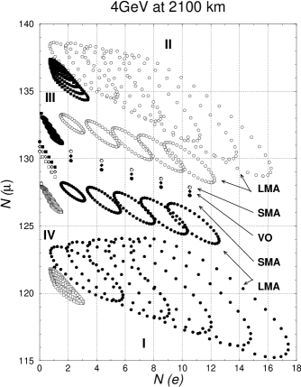
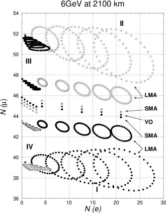
Figure 3: The neutrino parameter dependence of the expected event numbers for the NBB with $E_{p}=4$GeV(left) and 6GeV(right) and for 100ktyear at Beijing.

6 Summary

In this paper, we study the prospects of very long base-line (VLBL) neutrino-oscillation experiments with the High Intensity Proton Accelerator (HIPA). We present results for a VLBL experiment between HIPA and Beijing, where the base-line length is about 2100 km. We propose to use conventional pulsed-narrow-band $\nu_{\mu}$ beams and a huge water-Cherenkov detector of 100kt in mass. The detector should distinguish e-like, $\mu$-like and neutral current events but it is not required to measure the neutrino-energy. We study the sensitivity of such an experiment to the signs and the magnitudes of the neutrino mass-squared differences, the mixing angles, and the $CP$ phase of the $3\times 3$ lepton flavor mixing matrix (MNS matrix), by using the $\nu_{\mu}\to\nu_{e}$ transition probability and the $\nu_{\mu}$ survival probability. We find that the neutrino mass hierarchies can be determined from this experiment within several years. The $CP$ phase can be measured if both the mass-squared difference and all the mixing angles of the MNS matrix are sufficiently large.

References

References

- [1] JHF Neutrino Working Group, their web-site is http://neutrino.kek.jp/jhfnu.
- [2] Z.Maki, M.Nakagawa and S.Sakata, Prog. Theor. Phys. 28, 870 (1962)
- [3] LSND Collaboration, Phys. Pev. Lett. 77, 3082 (1996); Phys. Pev. Lett. 81, 1774 (1998).
- [4] K. Hagiwara and N. Okamura, Nucl. Phys. B548, 60 (1999).
- [5] Kamiokande Collaboration, K.S. Hirata et al., Phys. Lett. B205, 416 (1988); ibid. B280, 146 (1992); Y. Fukuda et al., Phys. Lett. B335, 237 (1994); IMB Collaboration, D. Casper et al., Phys. Pev. Lett. 66, 2561 (1991); R. Becker-Szendy et al., Phys. Rev. D46, 3720 (1992); SOUDAN2 Collaboration, T. Kafka, Nucl. Phys. (Proc. Suppl.) B35, 427 (1994); M.C. Goodman, ibid. 38, (1995) 337; W.W.M. Allison et al., Phys. Lett. B391, 491 (1997); hep-ex/9901024. Super-Kamiokande Collaboration, Phys. Pev. Lett. 81, 1562 (1998); Phys. Pev. Lett. 82, 2644 (1999); hep-ex/9903047.
- [6] Super-Kamiokande Collaboration, T. Toshito, talk at the ICHEP 2000, July 27 - August 2, 2000 at Osaka, Japan.
- [7] Homestake Collaboration, B.T. Cleveland et al., Nucl. Phys. (Proc. Suppl.) B38, 47 (1995); Ap. J. 496, 505 (1998); Kamiokande Collaboration, Y. Fukuda et al., Phys. Pev. Lett. 77, 1683 (1996); GALLEX Collaboration, W. Hampel et al., Phys. Lett. B388, 384 (1996); SAGE Collaboration, J.N. Abdurashitov et al., Phys. Pev. Lett. 77, 4708 (1996); Super-Kamiokande Collaboration, Y. Fukuda et al., Phys. Pev. Lett. 81, 1158 (1998), Phys. Pev. Lett. 82, 1810 (1999).
- [8] Super-Kamiokande Collaboration, Y. Takeuchi, talk at the ICHEP 2000, July 27 - August 2, 2000 at Osaka, Japan.
- [9] L. Wolfenstein, Phys. Rev. D17, 2369 (1978); S.P. Mikheyev and A.Yu. Smirnov, Yad. Fiz. 42, 1441 (1985) [Sov.J.Nucl.Phys.42, 913 (1986)]; Nuovo Cimento C9, 17 (1986).
- [10] B.Pontecorvo, Zh.Eksp. Teor. Fiz. 53, 1717 (1967); S.M. Bilenky and B. Pontecorvo, Phys. Rep. 41, 225 (1978); V.Barger, R.J.N. Phillips and K. Whisnant, Phys. Rev. D24, 538 (1981); S.L. Glashow and L.M. Krauss, Phys. Lett. 190B, 199 (1987).
- [11] The CHOOZ Collaboration, Phys. Lett. B420, 397 (1998); M. Apollonio et al., Phys. Lett. B466, 415 (1999).
- [12] C. Jarlskog, Phys. Pev. Lett. 55, 1039 (1985) and Z. Phys. C29, 491 (1985).