Abstract

Though the minimal model of anomaly mediated supersymmetry breaking has been significantly constrained by recent experimental and theoretical work, there are still allowed regions of the parameter space for moderate to large values of $\tan\beta$. We show that these regions will be comprehensively probed in a ${\sqrt{s}}=1$ TeV $e^{+}e^{-}$ linear collider. Diagnostic signals to this end are studied by zeroing in on a unique and distinct feature of a large class of models in this genre: a neutral winolike Lightest Supersymmetric Particle closely degenerate in mass with a winolike chargino. The pair production processes $e^{+}e^{-}\rightarrow{\tilde{e}}_{L}^{\pm}{\tilde{e}}_{L}^{\mp}$, ${\tilde{e}}_{R}^{\pm}{\tilde{e}}_{R}^{\mp}$, ${\tilde{e}}_{L}^{\pm}{\tilde{e}}_{R}^{\mp}$, ${\tilde{\nu}}{\bar{\tilde{\nu}}}$, $\widetilde{\chi}^{0}_{1}\widetilde{\chi}^{0}_{2}$, $\widetilde{\chi}^{0}_{2}\widetilde{\chi}^{0}_{2}$ are all considered at $\sqrt{s}=1$ TeV corresponding to the proposed TESLA linear collider in two natural categories of mass ordering in the sparticle spectra. The signals analysed comprise multiple combinations of fast charged leptons (any of which can act as the trigger) plus displaced vertices $X_{D}$ (any of which can be identified by a heavy ionizing track terminating in the detector) and/or associated soft pions with characteristic momentum distributions.

1 Introduction

The Minimal Supersymmetric Standard Model (MSSM [1]), with softly broken N=1 supersymmetry, is the prime candidate today for physics beyond the Standard Model (SM). Suppose the soft supersymmetry breaking terms explicitly appearing in the MSSM Lagrangian are regarded as low energy remnants of a spontaneous or dynamical breaking of supersymmetry at a high scale. We then know that the latter cannot take place in the observable sector of MSSM fields; it must occur in a hidden or secluded sector which is generally a singlet under SM gauge transformations. Though the precise mechanism of how supersymmetry breaking is transmitted to the observable sector of MSSM superfields is unknown, signals of supersymmetry in collider experiments sometimes depend sensitively on it. There are several different ideas of transmission, such as gravitational mediation at the tree level [2] and gauge mediation [3], each with its distinct signatures. A very interesting recent idea, that is different from the above two, is that of Anomaly Mediated Supersymmetry Breaking (AMSB) [4, 5] which is explained below. This scenario has led to a whole class of models and their phenomenological implications have been discussed [References - References], but let us confine ourselves here to the minimal version [4]. The latter has characteristically distinct and unique laboratory signatures. These have been explored in some detail for hadronic collider processes [References - References]. But there are also quite striking signals that such models predict for processes to be studied in a high energy $e^{+}e^{-}$ (or $\mu^{+}\mu^{-}$) linear collider [14]. This paper aims to provide a first detailed study of such signals in this type of a machine.

In ordinary gravity-mediated supersymmetry breaking tree level exchanges with gravitational couplings between the hidden and the observable sectors transmit supersymmetry breaking from one to the other. If $\Lambda_{ss}$ is the scale of spontaneous or dynamical breaking of supersymmetry in the hidden sector, explicit supersymmetry violating mass parameters of order $M_{s}\equiv\Lambda^{2}_{ss}M^{-1}_{pl}$, $M_{pl}$ being the reduced Planck mass $\sim 2\times 10^{18}$ GeV, get generated in the MSSM Lagrangian. However, in general, there are uncontrolled flavour changing neutral current (FCNC) amplitudes in this scenario. Though gravity is flavour blind, the supergravity invariance of the Lagrangian still admits direct interaction terms between the hidden and the observable sectors, such as

$${\cal L}_{eff}\simeq\int d^{4}\theta{h\over{M^{2}_{pl}}}\Sigma^{\dagger}\Sigma Q^{\dagger}Q.$$ (1)

In Eq. (1), $\Sigma$ and $Q$ are generic chiral superfields in the hidden and the observable sectors respectively, while $h$ is a dimensionless coupling of order unity. When supersymmetry is broken in the hidden sector, say through a nonzero vacuum expectation value $\langle F_{\Sigma}\rangle$ of the auxiliary component, masses get induced for spin zero sparticles in the observable sector. There is no symmetry to keep $h$ diagonal in flavour space. As a result, the squark soft mass matrix can have significant off-diagonal terms in that space, leading to a major conflict with strong experimental upper bounds on FCNC amplitudes from $K-{\bar{K}}$ and $B-{\bar{B}}$ mixing as well as from unobserved $\mu\rightarrow e\gamma$ decay and $\mu\rightarrow e$ conversions in nuclei [24].

Attempts to solve the above mentioned flavour problem have generally required special family symmetries [25] in addition to supergravity. In the alternative scenario [3], namely gauge mediated supersymmetry breaking, FCNC amplitudes are naturally absent. However, models of that category have other difficulties like the CP problem and the $\mu$ vs $\mu B$ ($\mu$ and $B$ being the higgsino mass and the Higgs sector supersymmetry violating parameters respectively) problem which are less severe in gravity-mediated scenarios. It is in this context that the recently proposed AMSB scenario has right away become interesting. Anomaly mediation is in fact a special case of gravity mediation where there are no direct tree level couplings between the superfields of the hidden and the observable sectors that convey supersymmetry breaking. This is realized, for instance, when the hidden and the observable sector superfields are localized on two parallel but distinct 3-branes located in a higher dimensional bulk as schematically depicted in Fig. 1.

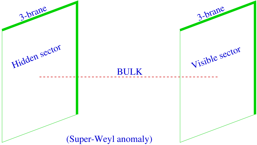
Figure 1: Supersymmetry breaking across the extra dimension(s).

Suppose that the two branes are separated by the bulk distance $\sim r_{c}$ where $r_{c}$ is the compactification radius. Then any tree level exchange with bulk fields of mass $m$ ($>r_{c}^{-1}$) will be suppressed by the factor $e^{-mr_{c}}$. Supergravity fields propagate in the bulk, but the supergravity-mediated tree level couplings can now be eliminated by a rescaling transformation. The problem can be considered in the background of a conformal compensator superfield $\Phi$ whose VEV is given [4] by $\langle\Phi\rangle$ = 1 + $m_{3/2}\theta\theta$, $m_{3/2}$ being the gravitino mass. The rescaling transformation is then given by $Q\Phi\rightarrow Q$. However, this rescaling symmetry is anomalous at the quantum level and the communication of supersymmetry breaking from the hidden to the observable sector takes place through the loop-generated superconformal anomaly. The latter is topological in origin and naturally conserves flavour so that no new FCNC amplitudes are introduced from supersymmetry breaking terms. Thus other advantages of gravity mediated supersymmetry breaking are retained in the AMSB scenario while the flavour problem is solved.

Let us assume that all explicit soft supersymmetry breaking parameters of the MSSM originate from AMSB. Then the masses of the gauginos and of the scalars get generated at the same order in the corresponding gauge coupling strengths. Therefore these masses are not expected to be very different. The expressions for the said quantities, in fact, become renormalization group invariant with sleptons becoming tachyonic. The latter fact is the most severe problem in the AMSB scenario and there are several proposals in the literature to solve it. We shall focus on the minimal [4] model of AMSB where the problem of tachyonic sleptons is tackled by adding a universal constant term $m^{2}_{0}$ to the expressions for squared scalar masses, i.e., $m^{2}_{0}$ contributes equally to the squared masses of all scalars present in the theory. One can now solve the tachyonic slepton problem through a suitably chosen $m^{2}_{0}$ making all squared slepton masses positive, the scale invariance of the expressions for scalar masses being lost. The evolution of scalar masses governed by the corresponding renormalization group equations (RGE), starting from a very high energy scale, must therefore be taken into account. However, except for the addition of an extra parameter, this is quite a feasible procedure. Recently, a mechanism to generate the minimal AMSB spectrum (including the universal additive constant $m^{2}_{0}$ in all squared scalar masses) has been proposed [23]. In this scheme only the SM matter superfields are confined to the 3-brane of the observable sector while the gauge superfields live in the bulk along with gravity. The presence of gauge and gaugino fields in the bulk results in the additional universal supersymmetry breaking contribution to all scalar masses squared. This contribution is naturally of the same size as its anomaly-induced counterparts.

One can say, on the basis of this last discussion, that the minimal AMSB model has now been soundly formulated and is worthy of serious consideration. Indeed, its parameter space has been severely constrained [References - References] by recent measurements of the $g-2$ of the muon [30] and of the branching fraction for the decay $B\rightarrow X_{s}\gamma$, but some regions of the parameter space still survive. This model is characterized by several distinct features with important phenomenological consequences: a rather massive gravitino ($\sim$ a few TeV) and nearly mass-degenerate left and right selectrons and smuons while the staus split into two distinct mass eigenstates with the ${\tilde{\tau}}_{1}$ being the lightest charged slepton. Most importantly, the model has gaugino masses proportional to the $\beta$-functions of the gauge couplings. The latter leads to the existence of a neutral near-Wino as the lightest supersymmetric particle (LSP) $\widetilde{\chi}_{1}^{0}$ and closely mass-degenerate with it a pair of charged near-Winos as the lighter charginos $\widetilde{\chi}_{1}^{\pm}$. A tiny mass difference $\Delta M$ $(<1$ GeV) arises between them from loop corrections and a weak gaugino-higgsino mixing at the tree level. Because of the small magnitude of $\Delta M$, $\widetilde{\chi}_{1}^{\pm}$, if produced in a detector, will be long-lived. Such a chargino then is likely to leave [31] a displaced vertex $X_{D}$ and/or a characteristic soft pion from the decay $\widetilde{\chi}_{1}^{\pm}\rightarrow\widetilde{\chi}_{1}^{0}+\pi^{\pm}$.

The pair production of MSSM sparticles and their decays which are characteristic of AMSB scenarios, have been considered in various theoretical studies conducted with respect to experiments in a hadronic collider [References - References]. But the same can be carried out for electron and muon colliders too [14]. Let us specifically take an $e^{+}e^{-}$ linear collider at a CM energy $\sqrt{s}=1$ TeV; the reason for such a choice will be explained below. We consider pair production processes such as $e^{+}e^{-}\rightarrow{\tilde{e}}_{L}^{\pm}{\tilde{e}}_{L}^{\mp}$, ${\tilde{e}}_{R}^{\pm}{\tilde{e}}_{R}^{\mp}$, ${\tilde{e}}_{L}^{\pm}{\tilde{e}}_{R}^{\mp}$, $\tilde{\nu}\bar{\tilde{\nu}}$, $\widetilde{\chi}_{1}^{0}\widetilde{\chi}_{2}^{0}$, $\widetilde{\chi}_{2}^{0}\widetilde{\chi}_{2}^{0}$. One could also produce smuon or stau pairs and look at the signals coming from their cascade decays. In case of smuons the event rates would be reduced typically by a factor of five on account of $s$-channel suppression. This is the reason why we have not explicitly considered smuon pair production here, though one can look for it in principle. A similar argument holds for stau pair production. Also, for the sake of simplicity, we choose not to consider taus in the final state here because of the lesser experimental efficiency in identifying them. There are broadly two types of AMSB mass spectra which we call Spectrum A and Spectrum B, to be described later. The cascade decay chains of the produced sparticles are different for the two spectra. We consider both spectra in detail and provide quantitative discussions of signals with final states containing multiple combinations of $X_{D}$/soft pions and fast charged leptons in both cases. As mentioned earlier, significant constraints [References - References] on the minimal AMSB model have been derived recently from measurements of the rare deay rate $\Gamma(B\rightarrow X_{s}\gamma)$ and of the muon anomalous magnetic moment ${(g-2)}_{\mu}$. Specifically, negative values of the Higgsino mass parameter $\mu$ have been effectively ruled out. However, we shall show that some regions of the AMSB parameter space are still allowed for moderate to large values of $\tan\beta$ (the ratio of the two Higgs VEVs). These are precisely the regions that we target in our studies. Moreover, the required absence of charge and colour violating global minima suggests [32] that charged sleptons in the minimal AMSB model are rather heavy and beyond the reach of a ${\sqrt{s}}=500$ GeV linear collider, the proposed JLC and NLC machines. It is interesting to note that the region still allowed by the ${(g-2)}_{\mu}$ and the $B\rightarrow X_{s}\gamma$ constraints is almost the one allowed from more theoretically motivated stability conditions. This is why we have chosen a $\sqrt{s}$ value of 1 TeV, to be attained by a linear collider such as the proposed TESLA [33]. Charged sleptons of the minimal AMSB model are therefore likely to be above (within) the kinematic reach of the former (latter) machine.

There have, of course, been other proposed models to solve the problem of tachyonic sleptons [References - References]. In most of these, however, the sparticle mass spectrum differs from that of the minimal model both in the gaugino as well as in the scalar sector. Since we are interested only in a near-Wino LSP scenario, we shall not discuss the phenomenology associated with those models which lack this feature. The near-Wino LSP feature is retained, however, in models invoking additional $D$-term contributions to soft scalar masses [References - References] keeping the sum of squared scalar masses RG invariant. This is because the mass spectrum in the gaugino sector remains the same as in the minimal AMSB model. Thus such schemes will lead finally to the kind of signals in a high energy $e^{+}e^{-}$ linear collider that we are going to discuss in the minimal model. However, the extreme degeneracy of the right and left selectrons (smuons) is lost here with the right becoming heavier. This feature can change the patterns of the cascade decays of various sparticles leading to observable consequences different from those of the minimal model. We shall discuss these complications separately.

The paper is organized as follows. In section 2 we describe and discuss the mass spectra of the minimal AMSB model and distinguish between the two cases A and B. In section 3, we enumerate processes of the pair production of different sleptons and neutralinos, as mentioned earlier; we also consider the relevant cascade decay chains that lead to our desired signals. The numerical results of these computations are presented in section 4 which also contains discussions of the results. The final section 5 provides a brief summary of our conclusions.

2 Spectra and Couplings of the Minimal AMSB Model

Scalar masses in the minimal AMSB model are determined via the RGE equations of the MSSM with appropriate boundary conditions at the gauge coupling unification scale $M_{G}\sim(1.5-2.0)\times 10^{16}~{}{\rm GeV}$. In the present analysis, the evolution of gauge and Yukawa couplings as well as that of scalar mass parameters are computed using two-loop RGE equations [34]. We have also incorporated the unification of gauge couplings at that scale with $\alpha_{3}(M_{Z})\approx 0.118$. The magnitude of the higgsino mass parameter $\mu$ gets fixed from the requirement of a radiative electroweak symmetry breaking. It is computed at the complete one-loop level of the effective potential [35], the optimal choice for the renormalization scale being $Q=\sqrt{(m_{{\tilde{t}}_{1}}m_{{\tilde{t}}_{2}})}$, $m_{{\tilde{t}}_{1}}(m_{{\tilde{t}}_{2}})$ being the lighter (heavier) stop mass. We have also included a supersymmetric QCD correction to the bottom-quark mass [36], which is significant for large $\tan\beta$. The model has only four parameters: the gravitino mass $m_{3/2}$, the common scalar mass parameter $m_{0}$, $\tan\beta$ and sgn($\mu$). However, we exclude the case $\mu<0$ since that has now been ruled out [26] by the recent ${(g-2)}_{\mu}$ data. The appropriate boundary conditions at the GUT scale for the masses and the trilinear couplings are given below. It should be re-emphasized at this point that gaugino masses and trilinear scalar couplings can be computed from these expressions at any scale once the appropriate values of the gauge ($g$) and Yukawa ($h$) couplings at that scale are known. We shall ignore Yukawa terms in the superpotential (and also the trilinear scalar couplings) pertaining to the first two generations, though not those involving the third generation. Sfermions of the heaviest family are therefore treated differently from those of the two lighter ones.

The scale invariant one-loop gaugino mass expressions are

$$M_{i}=b_{i}{g^{2}_{i}\over 16\pi^{2}}m_{3/2}.$$ (2)

where $b_{1}=33/5$, $b_{2}=1$, $b_{3}=-3$. To leading order, $M_{1,2,3}$ are independent of $m_{0}$ and increase linearly with $m_{3/2}$. Furthermore, at one-loop level the squared masses for the Higgs and third generation scalars are

$$m^{2}_{i}=C_{i}{m^{2}_{3/2}\over{(16\pi^{2})}^{2}}+m^{2}_{0},$$ (3)

where $i\equiv(Q,{\bar{U}},{\bar{D}},L,{\bar{E}},H_{u},H_{d})$ in standard notation, with the $C_{i}$’s being given as

$$C_{Q} = -{11\over 50}g^{4}_{1}-{3\over 2}g^{4}_{2}+8g^{4}_{3}+h_{t}{\hat{\beta}}_{h_{t}}+h_{b}{\hat{\beta}}_{h_{b}},$$

$$C_{\bar{U}} = -{88\over 25}g^{4}_{1}+8g^{4}_{3}+2h_{t}{\hat{\beta}}_{h_{t}},$$

$$C_{\bar{D}} = -{22\over 25}g^{4}_{1}+8g^{4}_{3}+2h_{b}{\hat{\beta}}_{h_{b}},$$

$$C_{L} = -{99\over 50}g^{4}_{1}-{3\over 2}g^{4}_{2}+h_{\tau}{\hat{\beta}}_{h_{\tau}},$$ (4)

$$C_{\bar{E}} = -{198\over 25}g^{4}_{1}+2h_{\tau}{\hat{\beta}}_{h_{\tau}},$$

$$C_{H_{u}} = -{99\over 50}g^{4}_{1}-{3\over 2}g^{4}_{2}+3h_{t}{\hat{\beta}}_{h_{t}},$$

$$C_{H_{d}} = -{99\over 50}g^{4}_{1}-{3\over 2}g^{4}_{2}+3h_{b}{\hat{\beta}}_{h_{b}}+h_{\tau}{\hat{\beta}}_{h_{\tau}}.$$

In Eqs. (2), $Q$ and $L$ refer to the respective squark and slepton $SU(2)$ doublet superfields, while ${\bar{U}}$, ${\bar{D}}$ and ${\bar{E}}$ stand for the singlet up-squark, down-squark and charged slepton superfields respectively and $H_{u}$ ($H_{d}$) describes the up-type (down-type) Higgs superfield. Moreover, the ${\hat{\beta}}$’s are given by

$$\hat{\beta}={(16\pi^{2})}^{-1}\beta,$$ (5)

where $\beta$ is the usual beta-function. Thus

$${\hat{\beta}}_{h_{t}} = h_{t}\left(-{13\over 15}g^{2}_{1}-3g^{2}_{2}-{16\over 3}g^{2}_{3}+6h^{2}_{t}+h^{2}_{b}\right),$$

$${\hat{\beta}}_{h_{b}} = h_{b}\left(-{7\over 15}g^{2}_{1}-3g^{2}_{2}-{16\over 3}g^{2}_{3}+h^{2}_{t}+6h^{2}_{b}+h^{2}_{\tau}\right),$$

$${\hat{\beta}}_{h_{\tau}} = h_{\tau}\left(-{9\over 5}g^{2}_{1}-3g^{2}_{2}+3h^{2}_{b}+4h^{2}_{\tau}\right).$$

Finally, the scale invariant expressions for the third generation trilinear $A$ couplings are

$$A_{t}={{\hat{\beta}}_{h_{t}}\over h_{t}}{m_{3/2}\over 16\pi^{2}},~{}A_{b}={{\hat{\beta}}_{h_{b}}\over h_{b}}{m_{3/2}\over 16\pi^{2}},~{}A_{\tau}={{\hat{\beta}}_{h_{\tau}}\over h_{\tau}}{m_{3/2}\over 16\pi^{2}}.$$ (6)

The expressions for sfermion masses and $A$-parameters of the first two generations can be obtained from the above by simply dropping the Yukawa couplings.

One of the interesting features of the minimal AMSB model is that the ratios of the respective $SU(3)$, $SU(2)$ and $U(1)$ gaugino mass parameters $M_{3}$, $M_{2}$ and $M_{1}$ are given, after taking into account the next to leading order (NLO) corrections and the weak scale threshold corrections [9], by

$$|M_{1}|:|M_{2}|:|M_{3}|=2.8:1:7.1$$ (7)

(Note that eq. (7), as deduced in [9], is true only for low and moderate values of $\tan\beta$. For large values of $\tan\beta$ where bottom and $\tau$ Yukawa couplings are nonnegligible, the ratio $|M_{1}|/|M_{2}|$ slightly increases [13].) As a result of eq. (7), the lighter chargino $\widetilde{\chi}_{1}^{\pm}$ and the lightest neutralino $\widetilde{\chi}_{1}^{0}$ become almost degenerate. The small difference in the masses, with the lightest neutralino being the lightest supersymmetric particle (LSP), comes from the tree-level gaugino-higgsino mixing as well as from the one-loop corrected chargino and the neutralino mass matrix. The small mass-splitting $\Delta M$ can be approximately written as

$$\Delta M=\frac{M_{W}^{4}\tan^{2}\theta_{W}}{(M_{1}-M_{2})\mu^{2}}\sin^{2}2\beta\bigg{[}1+{\cal O}\left(\frac{M_{2}}{\mu},\frac{M^{2}_{W}}{\mu M_{1}}\right)\bigg{]}$$

$$+\frac{\alpha M_{2}}{\pi\sin^{2}\theta_{W}}\bigg{[}f\left(\frac{M_{W}^{2}}{M_{2}^{2}}\right)-\cos^{2}\theta_{W}f\left(\frac{M_{Z}^{2}}{M_{2}^{2}}\right)\bigg{]},$$ (8)

with

$$f(x)\equiv-\frac{x}{4}+\frac{x^{2}}{8}\ln(x)+\frac{1}{2}\left(1+\frac{x}{2}\right)\sqrt{4x-x^{2}}\bigg{[}\tan^{-1}\left(\frac{2-x}{\sqrt{4x-x^{2}}}\right)-\tan^{-1}\left(\frac{x}{\sqrt{4x-x^{2}}}\right)\bigg{]}$$

The second term in the RHS of eq. (8) is the one-loop contribution which is dominated by gauge boson loops.

Figure 2: Mass difference $\Delta M$ between the lighter chargino ($\widetilde{\chi}_{1}^{\pm}$) and the LSP ($\widetilde{\chi}_{1}^{0}$) as a function of the gravitino mass ($m_{3/2}$) for $\tan\beta=10$ (upper curve) and $\tan\beta=30$ (lower curve), $\mu>0$ and $m_{0}=450$ GeV.

We have numerically investigated the mass-splitting $\Delta M$ in various region of the parameter space. Given the LEP lower limit [37] of 86 GeV on the mass of the lighter chargino for nearly degenerate $\widetilde{\chi}_{1}^{\pm}$-$\widetilde{\chi}_{1}^{0}$, it can be concluded that the upper limit on $\Delta M$ cannot be much in excess of $500~{}{\rm MeV}$. On the other hand, the condition of radiative electroweak symmetry breaking in the AMSB scenario gives the ratio $|\mu/M_{2}|$ to be approximately between 3 and 6. For very large $M_{2}$ (i.e. for very large $\mu$) the mass difference $\Delta M$ reaches an asymptotic value of $\approx 165$ MeV. Fig. 2 shows the typical variation of $\Delta M$ as a function of $m_{3/2}$ for a choice of $\mu>0$ and $m_{0}=450$ GeV. The two choices of $\tan\beta$ are shown in the figure. The curve is cut off on the left by the lower bound on $m_{3/2}$ implied by the experimental constraint [37] on the $\widetilde{\chi}_{1}^{\pm}$ mass ($m_{\widetilde{\chi}_{1}^{\pm}}>86$ GeV) for the nearly degenerate $\widetilde{\chi}_{1}^{\pm}$-$\widetilde{\chi}_{1}^{0}$ case. On the right, it gets terminated because otherwise the stau becomes the LSP with a further increase in $m_{3/2}$ for this particular value of $m_{0}$. This is also the reason why we have not been able to show the limiting value of $\Delta M\approx 165$ MeV on this plot.

In Fig. 3, we show a sample plot of various sparticle contours in the $m_{0}-m_{3/2}$ plane for two different choices of the other parameter, namely $\tan\beta$. The sign of $\mu$ has been taken to be positive. One of the very striking features of the minimal AMSB model is the strong mass degeneracy between the left and right charged sleptons. As a result of this, the third and the second generation L-R mixing angles become substantial. They can reach the maximal limit provided $\tan\beta$ is large. This large L-R mixing of the smuons has been shown to have a strong influence on the neutralino loop contribution (which is a rather small effect as compared to the dominant chargino loop contribution) to ${(g-2)}_{\mu}$ [38] in the context of the minimal AMSB scenario. The corresponding constraint on the parameter space has been derived assuming that the supersymmetric contribution to ${(g-2)}_{\mu}$ is restricted within a 2$\sigma$ limit of the combined error from the Standard Model calculation and from the current uncertainty in the Brookhaven measurement [References - References]. A similar constraint [26, 28] from the measured radiative decay rate $\Gamma(B\rightarrow X_{s}\gamma)$ has been invoked.

The top left corners of both the diagrams in Fig. 3, marked by $X$, are not allowed. This is due to the twin requirements of ${\tilde{\tau}}_{1}$ not being allowed to be the LSP and $m_{{\tilde{\tau}}_{1}}$ having to exceed the experimental lower bound of $70$ GeV [39]. Any further increase in $m_{3/2}$ for a particular value of $m_{0}$ is disallowed since then the staus become tachyonic. Furthermore, the lower limit on $m_{3/2}$ in each figure comes from the experimental constraint [37] $m_{\widetilde{\chi}_{1}^{\pm}}>86$ GeV. One can also check that the maximum possible value of $m_{3/2}$ for a given $m_{0}$ is a decreasing function of $\tan\beta$ [38]. Recently, new bounds on minimal AMSB model parameters have been proposed from the condition that the electroweak symmetry breaking minimum of the scalar potential is the deepest point in the field space [32]. Selected parameters for our entire numerical calculation have been chosen so as to be consistent with all these bounds.

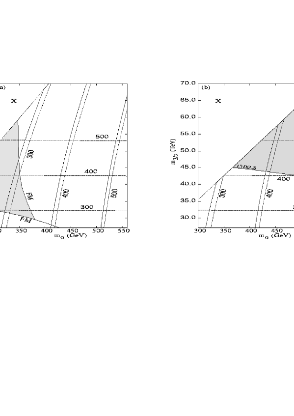
Figure 3: Contours of constant charged slepton (continuous) and sneutrino (dashed) masses in the $m_{0}-m_{3/2}$ plane for (a) $\tan\beta=10$ and $\mu>0$, (b) $\tan\beta=30$ and $\mu>0$. The number adjacent to each pair of curved lines corresponds to the sneutrino (slepton) mass for that particular contour. The dotted horizontal lines are the contours of constant $\widetilde{\chi}_{2}^{0}$ mass. The number adjacent to each horizontal line is the mass of $\widetilde{\chi}_{2}^{0}$ for that contour. The boundaries of constraint, labelled by FM and CHKLS (the near vertical boundary in (a) from ${(g-2)}_{\mu}$ and the near horizontal boundaries in (a) and (b) from $\Gamma(B\rightarrow X_{s}\gamma)$), have been taken from Refs. [26] and [28] respectively. The shaded regions are the allowed regions in the two figures.

The continuous and dashed curved lines in Fig. 3 stand for contours of constant charged slepton and sneutrino masses respectively . It is easy to see why the latter are lower than the former. The sneutrino mass is linked with the left charged slepton mass through the $SU(2)_{L}$ relation

$$m^{2}_{\tilde{\nu}}=m^{2}_{\tilde{L}}+{1\over 2}m^{2}_{Z}cos2\beta.$$ (9)

Thus, for $\tan\beta>1$, $m_{\tilde{\nu}}$ is always smaller than $m_{\tilde{L}}$. Since the right and the left sleptons are very highly degenerate, sneutrinos are always lighter than the right sleptons too. The horizontal lines in Fig. 3 are contours of constant $\widetilde{\chi}_{2}^{0}$ mass. It may be noted that no $\widetilde{\chi}_{1}^{0}$ mass contour has entered these figures since the LSP $\widetilde{\chi}_{1}^{0}$ is always significantly lighter than $\widetilde{\chi}_{2}^{0}$. Depending on various parametric choices, we see that the AMSB sparticle mass spectrum can be broadly classified into two natural categories with mass ordering as given below (sparticle symbols standing for sparticle masses):

• Spectrum A: $\widetilde{\chi}_{1}^{0}(\approx\widetilde{\chi}_{1}^{\pm})<\tilde{\nu}<{\tilde{e}}_{R}(\approx{\tilde{e}}_{L})<\widetilde{\chi}_{2}^{0}$

• Spectrum B: $\widetilde{\chi}_{1}^{0}(\approx\widetilde{\chi}_{1}^{\pm})<\widetilde{\chi}_{2}^{0}<\tilde{\nu}<{\tilde{e}}_{R}(\approx{\tilde{e}}_{L}).$

Note that, in AMSB scenarios with a wino LSP, $\widetilde{\chi}_{2}^{\pm}$ and $\widetilde{\chi}^{0}_{3,4}$ are higgsino-dominated and heavy enough to be neglected in our signal studies. Also, for large values of $\tan\beta$, there exists a region where the mass of $\widetilde{\chi}_{2}^{0}$ is between that of the lighter stau $\tilde{\tau}_{1}$ and the first generation sleptons. This variant, which we call Spectrum B1, is characterized by

• Spectrum B1: $\widetilde{\chi}_{1}^{0}(\approx\widetilde{\chi}_{1}^{\pm})<\tilde{\tau}_{1}<\widetilde{\chi}_{2}^{0}<\tilde{\nu}<{\tilde{e}}_{R}(\approx{\tilde{e}}_{L}).$

For most of the decay modes, the spectra B and B1 have identical behaviour, and we do not list them separately. The only exception is the decay of $\widetilde{\chi}_{2}^{0}$, which is discussed in Section 3.2.

It can be seen from Fig. 3 that mass-orderings, other than A and B above, are allowed only in very restricted regions of the $m_{3/2}-m_{0}$ plane and correspond to the fine tuning of some parameters. This is why we do not consider them further. As already mentioned, staus and smuons are not considered for production here. That is the reason why we have not included them in the two classes of spectrum written above. (However, for completeness, one may note that the smuons are almost degenerate with the selectrons, while the lighter stau is the lightest slepton for large values of $\tan\beta$). Finally, the regions in the parameter space, where the LSP can be either the $\tilde{\tau}_{1}$ (the two stau mass eigenstates are separated because of the large off-diagonal terms in the stau mass matrix) or the sneutrino, are disfavoured on cosmological grounds. Such LSPs are also incompatible with the stability of the supersymmetric scalar potential [32]. Thus, there are really only two distinct classes of spectra which are relevant and interesting for our present study.

3 Production and Decays of Sparticles

The basic production processes that we consider are $e^{+}e^{-}\rightarrow{\tilde{e}}_{L}^{\pm}{\tilde{e}}_{L}^{\mp}$, ${\tilde{e}}_{R}^{\pm}{\tilde{e}}_{R}^{\mp}$, ${\tilde{e}}_{L}^{\pm}{\tilde{e}}_{R}^{\mp}$, ${\tilde{\nu}}{\bar{\tilde{\nu}}}$, $\widetilde{\chi}^{0}_{1}\widetilde{\chi}^{0}_{2}$, $\widetilde{\chi}^{0}_{2}\widetilde{\chi}^{0}_{2}$. We have not included the process $e^{+}e^{-}\rightarrow\widetilde{\chi}_{1}^{\pm}{\widetilde{\chi}_{1}^{\mp}}$ since that will yield two displaced vertices/soft pions in addition to $E_{T}/\;\>$; the only way to trigger the reaction would be to consider an additional initial-state-radiated (ISR) photon [31]. However, apart from the rate being lower by a factor $\alpha$, such a signal could also come from the light higgsino ($|\mu|\ll|M_{1,2}|$) scenario. The process $e^{+}e^{-}\rightarrow\chi_{1}^{+}\chi_{1}^{-}\gamma$ in the AMSB model has been discussed in Ref. [40]. Another possible process that we have not considered is the heavier $e^{+}e^{-}\rightarrow\widetilde{\chi}_{1}^{\pm}\tilde{\chi}^{\pm}_{2}$ since the dominant decay mode of $\tilde{\chi}^{\pm}_{2}$ in the AMSB scenario is $\tilde{\chi}^{\pm}_{2}\rightarrow\widetilde{\chi}_{1}^{\pm}h$ and then the branching ratio for a final configuration with multilepton + soft pion + $E_{T}/\;\>$ is rather small.

In this section we shall also enumerate all possible decay channels of the low-lying sparticles $\widetilde{\chi}_{1}^{\pm}$, $\widetilde{\chi}_{2}^{0}$, ${\tilde{e}}_{L}$, ${\tilde{e}}_{R}$ and $\tilde{\nu}$ that result in one or more leptons plus at least one soft charged pion accompanied by missing energy. Let us highlight some important characteristics, selection criteria and conventions that we have used.

• $\widetilde{\chi}_{1}^{\pm}$ and $\widetilde{\chi}_{1}^{0}$ are almost exclusively winos and $\widetilde{\chi}_{1}^{\pm}$ decays slowly (with a visibly displaced vertex $X_{D}$) only to $\widetilde{\chi}_{1}^{0}$ + soft $\pi^{\pm}$.

• $\widetilde{\chi}_{2}^{0}$ is almost a bino; at least, those decays that require a nonzero wino component of $\widetilde{\chi}_{2}^{0}$ are neglected, while the higgsino components are unimportant since we are considering only $e$ or $\mu$ in the final state. An exception is made for $\widetilde{\chi}_{2}^{0}$ decay in spectrum B, and is discussed in section 3.2.

• Whenever one or more two-body decay channels are kinematically allowed, we do not consider possible three- or four-body channels. Three-body channels, for instance, are significant only when no two-body decay channel exists and are considered only in that situation.

• Written without any suffix, $\tilde{\nu}$ and $\nu$ indicate both electron and muon-type sneutrinos. Similarly, $\ell$ ($\ell_{1}$, $\ell_{2}$) stands for $e$ or $\mu$. For simplicity, we do not consider any $\tau$ signals. We use the same notation for both (s)neutrino and anti(s)neutrino; they can be discriminated from the charge of the associated (s)lepton.

3.1 Decay cascade for Spectrum A

For Spectrum A, the allowed decay channels are as follows:

1. $\widetilde{\chi}_{2}^{0}\rightarrow\nu\tilde{\nu},~{}~{}~{}\ell_{L}^{\pm}{\tilde{\ell}}_{L}^{\mp},~{}~{}~{}\ell_{R}^{\pm}{\tilde{\ell}}_{R}^{\mp}$.

2. ${\tilde{e}}_{L}\rightarrow e\widetilde{\chi}_{1}^{0},~{}~{}\nu_{e}\widetilde{\chi}_{1}^{\pm}$.

3. ${\tilde{e}}_{R}\rightarrow e\widetilde{\chi}^{0*}_{2}\rightarrow e\nu\tilde{\nu}$. Note that ${\tilde{e}}_{R}$ must have a three-body decay since $\widetilde{\chi}_{1}^{0}$ has a vanishing bino component. Also, the virtual $\widetilde{\chi}^{0*}_{2}$ goes into the $\nu\tilde{\nu}$ channel rather than the $\ell_{L}^{\pm}{\tilde{\ell}}_{L}^{\mp}$ channel since ${\tilde{\ell}}_{L}$ is never lighter than ${\tilde{e}}_{R}$ in minimal AMSB. (In other AMSB models [References - References] where ${\tilde{e}}_{R}$ is heavier than ${\tilde{\ell}}_{L}$, this mode is also allowed.) However, the $\tau\tilde{\tau}_{1}$ channel, though included in the calculation of the branching fractions of other channels, is not considered explicitly since we do not look at final states with $\tau$’s.

4. $\tilde{\nu}\rightarrow\nu\widetilde{\chi}_{1}^{0},~{}~{}\ell^{\mp}\widetilde{\chi}_{1}^{\pm}$.

This immediately predicts the decay cascade for low-lying sparticles. As already pointed out, $\widetilde{\chi}_{1}^{\pm}$ results in a visibly displaced vertex $X_{D}$ and/or a soft charged pion. We club $\widetilde{\chi}_{1}^{0}$, which invariably appears at the end in sparticle dacays, and $\nu$ under $E_{T}/\;\>$. Thus, the end products of various sleptons and $\widetilde{\chi}_{2}^{0}$ are

1. $\tilde{\nu}\rightarrow\ell^{\pm}\pi^{\mp}E_{T}/\;\>$ (it can have a completely invisible mode $\tilde{\nu}\rightarrow\nu\widetilde{\chi}_{1}^{0}$ and thus can act as a virtual LSP).

2. ${\tilde{e}}_{L}\rightarrow eE_{T}/\;\>,~{}\pi E_{T}/\;\>$.

3. ${\tilde{e}}_{R}\rightarrow eE_{T}/\;\>,~{}e\ell^{\pm}\pi^{\mp}E_{T}/\;\>$.

4. $\widetilde{\chi}_{2}^{0}\rightarrow\ell^{\pm}\pi^{\mp}E_{T}/\;\>,~{}\ell^{+}\ell^{-}E_{T}/\;\>,~{}\ell_{1}^{+}\ell_{1}^{-}\ell_{2}^{\pm}\pi^{\mp}E_{T}/\;\>$ ($\ell_{1},\ell_{2}=e,\mu$).

We focus on the following six production processes in an $e^{+}e^{-}$ linear collider. Only those final states with one or two soft charged pions accompanied by at least one charged lepton and $E_{T}/\;\>$ are enlisted; however, only states with one soft pion, and dileptons with two soft pions, are discussed in detail in the next section. Note that some of the possible final states, e.g., five leptons and a soft pion, has negligibly small cross sections due to very small branching ratios in various stages of the cascade.

3.1.1 Production processes

Process 1: $e^{+}e^{-}\rightarrow\tilde{\nu}\bar{\tilde{\nu}}$ : Possible final states here are $\ell^{\pm}\pi^{\mp}$ or $\ell^{+}\ell^{-}\pi^{+}\pi^{-}$. The leptonic flavour is the flavour of the produced $\tilde{\nu}$; if we consider only $\tilde{\nu}_{e}$ pair production (which will be more copious than $\tilde{\nu}_{\mu}$ pair production due to the $t$-channel ${\tilde{e}}_{L}$ exchange diagram) the final state will have one or two electrons.

Process 2: $e^{+}e^{-}\rightarrow{\tilde{e}}_{L}^{+}{\tilde{e}}_{L}^{-}$ : The only possible signal here is $e^{\pm}\pi^{\mp}$.

Process 3: $e^{+}e^{-}\rightarrow{\tilde{e}}_{R}^{+}{\tilde{e}}_{R}^{-}$ : There can be two possible pionic final states in this case, namely, $e^{+}e^{-}\ell^{\pm}\pi^{\mp}$, and $e^{+}e^{-}\ell_{1}^{\pm}\ell_{2}^{\mp}\pi^{+}\pi^{-}$. Note that here $\ell_{1}$ and $\ell_{2}$ may be different since they come from the flavour-blind $\widetilde{\chi}_{2}^{0}$ decay. Thus, there are four possible combinations of two-pion final states.

Process 4: $e^{+}e^{-}\rightarrow{\tilde{e}}_{R}^{\pm}{\tilde{e}}_{L}^{\mp}$ : This process takes place only through the $t$-channel exchange of $\widetilde{\chi}_{2}^{0}$. The corresponding final states are $e^{\pm}\pi^{\mp}$, $e^{+}e^{-}\ell^{\pm}\pi^{\mp}$ and $e^{\pm}\ell^{\mp}\pi^{+}\pi^{-}$.

Process 5: $e^{+}e^{-}\rightarrow\widetilde{\chi}_{1}^{0}\widetilde{\chi}_{2}^{0}$ : The final state here is essentially that obtained from the cascade decay of $\widetilde{\chi}_{2}^{0}$. We will focus on only two generic channels, namely, $\ell^{\pm}\pi^{\mp}$ and $\ell_{1}^{+}\ell_{1}^{-}\ell_{2}^{\pm}\pi^{\mp}$ ($\ell_{1},\ell_{2}=e,\mu$). Depending on the flavours of $\ell_{1}$ and $\ell_{2}$, there are actually six channels.

Process 6: $e^{+}e^{-}\rightarrow\widetilde{\chi}_{2}^{0}\widetilde{\chi}_{2}^{0}$ : The pair production of $\widetilde{\chi}_{2}^{0}$ produces a rich variety of possible final states. Single pion final states include $\ell^{\pm}\pi^{\mp}$, $\ell_{1}^{\pm}\ell_{2}^{+}\ell_{2}^{-}\pi^{\mp}$ and $\ell_{1}^{\pm}\ell_{2}^{+}\ell_{2}^{-}\ell_{3}^{+}\ell_{3}^{-}\pi^{\mp}$. Note that every possible configuration necessarily has an odd number of charged leptons. Depending on the leptonic flavour, one has twelve channels with single soft pions plus one or more charged leptons plus $E_{T}/\;\>$. There are three two-pion final states with an even number of charged leptons: $\ell_{1}^{\pm}\ell_{2}^{\mp}\pi^{+}\pi^{-}$, $\ell_{1}^{\pm}\ell_{2}^{+}\ell_{2}^{-}\ell_{3}^{\mp}\pi^{+}\pi^{-}$ and $\ell_{1}^{\pm}\ell_{2}^{+}\ell_{2}^{-}\ell_{3}^{+}\ell_{3}^{-}\ell_{4}^{\mp}\pi^{+}\pi^{-}$. These result in fifteen flavour-specific channels.

3.2 Decay cascade for Spectrum B

The allowed decay channels for Spectrum B are as follows:

1. ${\tilde{e}}_{L}\rightarrow e\widetilde{\chi}_{1}^{0},~{}~{}e\widetilde{\chi}_{2}^{0},~{}~{}\nu_{e}\widetilde{\chi}_{1}^{\pm}$.

2. ${\tilde{e}}_{R}\rightarrow e\widetilde{\chi}_{2}^{0}$. Thus ${\tilde{e}}_{R}$ has a more prompt decay in spectrum B than in spectrum A.

3. $\tilde{\nu}\rightarrow\nu\widetilde{\chi}_{1}^{0},~{}~{}\nu\widetilde{\chi}_{2}^{0},~{}~{}\ell^{\mp}\widetilde{\chi}_{1}^{\pm}$.

4. $\widetilde{\chi}_{2}^{0}$ does not have the two-body decay channel to a lepton and a slepton. Its dominant decay modes are: $\widetilde{\chi}_{2}^{0}\rightarrow\widetilde{\chi}_{1}^{0}h$, $\widetilde{\chi}_{2}^{0}\rightarrow\widetilde{\chi}_{1}^{0}Z$, $\widetilde{\chi}_{2}^{0}\rightarrow\widetilde{\chi}_{1}^{\pm}W^{\mp}$, where $h$ is the lightest CP-even Higgs scalar. The last two modes occur through the tiny wino and/or higgsino components of the predominantly binolike $\widetilde{\chi}_{2}^{0}$. Still, they dominate over the three-body decay channels mediated by virtual sneutrinos or left charged sleptons: $\widetilde{\chi}_{2}^{0}\rightarrow\nu\tilde{\nu}^{*}\rightarrow\nu\nu\widetilde{\chi}_{1}^{0},~{}\nu\ell^{\pm}\pi^{\mp}\widetilde{\chi}_{1}^{0}$; $\widetilde{\chi}_{2}^{0}\rightarrow\ell_{L}^{\pm}\tilde{\ell_{L}^{*}}^{\mp}\rightarrow\ell^{+}\ell^{-}\widetilde{\chi}_{1}^{0},~{}\ell^{\pm}\nu\pi^{\mp}\widetilde{\chi}_{1}^{0}$. Since an ${\tilde{\ell}}_{R}$ cannot decay into $\ell\widetilde{\chi}_{1}^{0}$, any ${\tilde{\ell}}_{R}$-mediated decay does not occur. The two-body modes are, of course, not kinematically suppressed; the mass limit of $\widetilde{\chi}_{1}^{\pm}$ governs the minimum mass splitting of $\widetilde{\chi}_{2}^{0}$ and $\widetilde{\chi}_{1}^{0}$ and precludes any such suppression.

   For Spectrum B1 (see the last paragraph of Section 2), the two body channel $\widetilde{\chi}_{2}^{0}\rightarrow\tau\tilde{\tau}_{1}$ opens up, and the branching ratios of all the above-mentioned two-body channels get suppressed. Since we are not looking at final states with $\tau$’s, it would be hard to detect a $\widetilde{\chi}_{2}^{0}$ in this case.

The decay cascades for sleptons and gauginos are:

1. $\widetilde{\chi}_{2}^{0}\rightarrow\ell^{\pm}\pi^{\mp}E_{T}/\;\>,~{}\ell^{+}\ell^{-}E_{T}/\;\>$. $\widetilde{\chi}_{2}^{0}$ also has a virtual LSP mode $\widetilde{\chi}_{2}^{0}\rightarrow\nu\nu\widetilde{\chi}_{1}^{0}$. The leptons come from the decay of $W$ and $Z$; $h$ decays dominantly into $b\bar{b}$ and $\tau\bar{\tau}$ which we do not consider here. Note that the three-body channels also give the same final states, albeit in a tiny fraction. As discussed earlier, the branching ratios for these modes suffer a heavy suppression once we look at Spectrum B1.

2. $\tilde{\nu}\rightarrow\ell^{\pm}\pi^{\mp}E_{T}/\;\>,~{}\ell^{+}\ell^{-}E_{T}/\;\>$ (and the virtual LSP mode listed for spectrum A).

3. ${\tilde{e}}_{L}\rightarrow eE_{T}/\;\>,~{}\pi E_{T}/\;\>,~{}e\ell^{+}\ell^{-}E_{T}/\;\>,~{}e\ell^{\pm}\pi^{\mp}E_{T}/\;\>$.

4. ${\tilde{e}}_{R}\rightarrow eE_{T}/\;\>,~{}e\ell^{+}\ell^{-}E_{T}/\;\>,~{}e\ell^{\pm}\pi^{\mp}E_{T}/\;\>$.

Next, we enlist the signals for the pair production of charged sleptons and gauginos. As stated earlier, our signals consist of one or more charged leptons (but no $\tau$) plus one or two soft charged pions, accompanied with $E_{T}/\;\>$.

3.2.1 Production processes

Process 1: $e^{+}e^{-}\rightarrow\tilde{\nu}\bar{\tilde{\nu}}$ : Possible one pion final states are $\ell^{\pm}\pi^{\mp}$ and $\ell_{1}^{+}\ell_{1}^{-}\ell_{2}^{\pm}\pi^{\mp}$, where $\ell_{1}$ and $\ell_{2}$ can both be $e$ or $\mu$ irrespective of the sneutrino flavour. Thus, there can be six flavour-specific final states. The only possible two-pion final state is $\ell_{1}^{\pm}\ell_{2}^{\mp}\pi^{+}\pi^{-}$, which actually is a combination of three flavour-specific channels.

Process 2: $e^{+}e^{-}\rightarrow{\tilde{e}}_{L}^{+}{\tilde{e}}_{L}^{-}$ : The one-pion final states are $\ell^{\pm}\pi^{\mp}$, $e^{+}e^{-}\ell^{\pm}\pi^{\mp}$, $e^{\pm}\ell^{+}\ell^{-}\pi^{\mp}$, and $e^{+}e^{-}\ell_{1}^{+}\ell_{1}^{-}\ell_{2}^{\pm}\pi^{\mp}$. Written in full, they indicate two one-lepton, three three-lepton and four five-lepton final states. The two-pion states are $e^{\pm}\ell^{\pm}\pi^{\mp}\pi^{\mp}$ (note that in this case we may have a like-sign dilepton signal) and $e^{+}e^{-}\ell_{1}^{\pm}\ell_{2}^{\pm}\pi^{\mp}\pi^{\mp}$ (this will result in a four-lepton signal, with three of them of the same sign).

Process 3: $e^{+}e^{-}\rightarrow{\tilde{e}}_{R}^{+}{\tilde{e}}_{R}^{-}$ : Right selectrons can only decay to $\widetilde{\chi}_{2}^{0}$, so the possible one-pion signals are $e^{+}e^{-}\ell^{\pm}\pi^{\mp}$ and $e^{+}e^{-}\ell_{1}^{+}\ell_{1}^{-}\ell_{2}^{\pm}\pi^{\mp}$. Altogether, they add up to six one-pion final states. The only possible two-pion state is $e^{+}e^{-}\ell_{1}^{\pm}\ell_{2}^{\pm}\pi^{\mp}\pi^{\mp}$.

Process 4: $e^{+}e^{-}\rightarrow{\tilde{e}}_{R}^{\pm}{\tilde{e}}_{L}^{\mp}$ : There are four generic one-pion final states for this associated production process, namely, $e^{\pm}\pi^{\mp}$, $e^{+}e^{-}\ell^{\pm}\pi^{\mp}$, $e^{\pm}\ell^{\pm}\ell^{\mp}\pi^{\mp}$ and $e^{+}e^{-}\ell_{1}^{+}\ell_{1}^{-}\ell_{2}^{\pm}\pi^{\mp}$, which result in eight flavour-specific channels. The two-pion final states can be $e^{\pm}\ell^{\pm}\pi^{\mp}\pi^{\mp}$ and $e^{+}e^{-}\ell_{1}^{\pm}\ell_{2}^{\pm}\pi^{\mp}\pi^{\mp}$.

Process 5: $e^{+}e^{-}\rightarrow\widetilde{\chi}_{1}^{0}\widetilde{\chi}_{2}^{0}$ : There is only one possible channel, viz. $\ell^{\pm}\pi^{\mp}$.

Process 6: $e^{+}e^{-}\rightarrow\widetilde{\chi}_{2}^{0}\widetilde{\chi}_{2}^{0}$ : Possible one-pion channels are $\ell^{\pm}\pi^{\mp}$ and $\ell_{1}^{+}\ell_{1}^{-}\ell_{2}^{\pm}\pi^{\mp}$, resulting in six channels altogether.

In the three-lepton channel, two leptons of opposite sign and identical flavour should have their invariant mass peaked at $m_{Z}$. The only possible two-pion channel is $\ell_{1}^{\pm}\ell_{2}^{\pm}\pi^{\mp}\pi^{\mp}$. Note that this decay may also give a like-sign dilepton signal.

Spectrum	Signals	Parent Channels
	$e~{}\pi$	$\tilde{\nu}\bar{\tilde{\nu}},~{}~{}{\tilde{e}}_{L}{\tilde{e}}_{L},~{}~{}{\tilde{e}}_{L}{\tilde{e}}_{R},~{}~{}\widetilde{\chi}_{1}^{0}\widetilde{\chi}_{2}^{0},~{}~{}\widetilde{\chi}_{2}^{0}\widetilde{\chi}_{2}^{0}$
	$\mu~{}\pi$	$\tilde{\nu}\bar{\tilde{\nu}},~{}~{}\widetilde{\chi}_{1}^{0}\widetilde{\chi}_{2}^{0},~{}~{}\widetilde{\chi}_{2}^{0}\widetilde{\chi}_{2}^{0}$
A	$e~{}e~{}\ell~{}\pi$	${\tilde{e}}_{R}{\tilde{e}}_{R},~{}~{}{\tilde{e}}_{L}{\tilde{e}}_{R},~{}~{}\widetilde{\chi}_{1}^{0}\widetilde{\chi}_{2}^{0},~{}~{}\widetilde{\chi}_{2}^{0}\widetilde{\chi}_{2}^{0}$
	$\mu~{}\mu~{}\ell~{}\pi$	$\widetilde{\chi}_{1}^{0}\widetilde{\chi}_{2}^{0},~{}~{}\widetilde{\chi}_{2}^{0}\widetilde{\chi}_{2}^{0}$
	$\ell_{1}~{}\ell_{1}~{}\ell_{2}~{}\ell_{2}~{}\ell_{3}~{}\pi$	$\widetilde{\chi}_{2}^{0}\widetilde{\chi}_{2}^{0}$ ($\ell_{1,2,3}=e,~{}\mu$)
	$e~{}\pi$	$\tilde{\nu}\bar{\tilde{\nu}},~{}~{}{\tilde{e}}_{L}{\tilde{e}}_{L},~{}~{}{\tilde{e}}_{L}{\tilde{e}}_{R},~{}~{}\widetilde{\chi}_{1}^{0}\widetilde{\chi}_{2}^{0},~{}~{}\widetilde{\chi}_{2}^{0}\widetilde{\chi}_{2}^{0}$
	$\mu~{}\pi$	$\tilde{\nu}\bar{\tilde{\nu}},~{}~{}{\tilde{e}}_{L}{\tilde{e}}_{L},~{}~{}\widetilde{\chi}_{1}^{0}\widetilde{\chi}_{2}^{0},~{}~{}\widetilde{\chi}_{2}^{0}\widetilde{\chi}_{2}^{0}$
B	$e~{}\ell_{1}~{}\ell_{2}~{}\pi$	${\tilde{e}}_{R}{\tilde{e}}_{R},~{}~{}{\tilde{e}}_{L}{\tilde{e}}_{R},~{}~{}{\tilde{e}}_{L}{\tilde{e}}_{L},~{}~{}\tilde{\nu}\bar{\tilde{\nu}},~{}~{}\widetilde{\chi}_{2}^{0}\widetilde{\chi}_{2}^{0}$
		($\ell_{1,2}=e,~{}\mu$)
	$\mu~{}\mu~{}\mu~{}\pi$	$\widetilde{\chi}_{2}^{0}\widetilde{\chi}_{2}^{0},~{}~{}\tilde{\nu}\bar{\tilde{\nu}}$
	$e~{}e~{}\ell_{1}~{}\ell_{1}~{}\ell_{2}~{}\pi$	${\tilde{e}}_{L}{\tilde{e}}_{L},~{}~{}{\tilde{e}}_{R}{\tilde{e}}_{R},~{}~{}{\tilde{e}}_{L}{\tilde{e}}_{R}$ ($\ell_{1,2}=e,~{}\mu$)

Table 1: Possible one or multilepton signal with one soft pion. All possible combinations of leptonic flavours are to be taken into account where the flavour is not shown explicitly.

A list of all possible final states and their parent sparticles, as discussed above, for both Spectra A and B, is given in Table 1 for one pion channels. A similar list is given in Table 2 for two pion channels. In the next section, we discuss some of the one-pion signals and the dilepton plus dipion signal, in detail, but let us note a few key features right at this point.

• One can sometimes have the same signal for Spectrum A or B; however, their sources are different. This means that the production cross-section and different distributions will also vary from one spectrum to the other; this may help discriminate between them. A useful option may be to use one polarized beam when some of the channels would be altogether ruled out.

• One must have an odd (even) number of charged leptons produced in conjunction with one (two) soft pion(s) in order to maintain charge neutrality. However, one can have a maximum of five leptons in the one-pion channel for both Spectra A and B. On the other hand, for two-pion channels, Spectrum A allows at most six charged leptons, while Spectrum B allows only four. The signal cross sections of the multilepton channels (with lepton number $\geq$ 4) may, however, be unobservably small with the presently designed luminosity of a $\sqrt{s}=1$ TeV linear collider.

• Three charged lepton plus one soft pion ($3\ell 1\pi$) signals are interesting in their own right. Consider the $3\mu 1\pi$ signal. For Spectrum B, two opposite sign muons must have their invariant mass peaked at $m_{Z}$, while no such compulsion exists for Spectrum A. This can serve as a useful discriminator between these two options.

• For signals with more than three charged leptons, one must have at least two electrons for Spectrum B, while all of them can be muons for Spectrum A. This can be directly traced to the fact that for Spectrum B a selectron pair is the parent whereas a $\widetilde{\chi}_{2}^{0}$ pair generates the multilepton signal in Spectrum A.

• For two-pion and two charged lepton final states, one may have more like-sign dileptons for Spectrum B than for Spectrum A. For one-pion states, one may get a stronger same-flavour like-sign dilepton signal for Spectrum B. The reasons are twofold: (a) Spectrum B gives $\widetilde{\chi}_{2}^{0}$ pairs more frequently at intermediate stages of the cascade and (b) $\widetilde{\chi}_{2}^{0}$ in Spectrum A is expected to be heavier than in Spectrum B. In fact, for Spectrum A $\widetilde{\chi}_{2}^{0}$ may even be outside the energy reach of the collider, in which case there will not be any like sign dilepton events in the final state.

• From theoretical considerations of charge and colour conservation, sleptons are expected [32] to be somewhat heavy in the minimal AMSB model. In fact, the lower bounds on their masses depend on the chargino mass.

Spectrum	Signals	Parent Channels
	$e~{}\ell~{}\pi~{}\pi$	$\tilde{\nu}\bar{\tilde{\nu}},~{}~{}{\tilde{e}}_{L}{\tilde{e}}_{R},~{}~{}\widetilde{\chi}_{2}^{0}\widetilde{\chi}_{2}^{0}$
	$\mu~{}\mu~{}\pi~{}\pi$	$\tilde{\nu}\bar{\tilde{\nu}},~{}~{}\widetilde{\chi}_{2}^{0}\widetilde{\chi}_{2}^{0}$
A	$e~{}e~{}\ell_{1}~{}\ell_{2}~{}\pi~{}\pi$	${\tilde{e}}_{R}{\tilde{e}}_{R},~{}~{}\widetilde{\chi}_{2}^{0}\widetilde{\chi}_{2}^{0}$ ($\ell_{1,2}=e,~{}\mu$)
	$\mu~{}\mu~{}\mu~{}\ell~{}\pi~{}\pi$	$\widetilde{\chi}_{2}^{0}\widetilde{\chi}_{2}^{0}$
	n $e$, (6-n) $\mu$, $\pi~{}\pi$	$\widetilde{\chi}_{2}^{0}\widetilde{\chi}_{2}^{0}$
	($0\leq{\rm n}\leq 6$)
	$e~{}\ell~{}\pi~{}\pi$	$\tilde{\nu}\bar{\tilde{\nu}},~{}~{}{\tilde{e}}_{L}{\tilde{e}}_{L},~{}~{}{\tilde{e}}_{L}{\tilde{e}}_{R},~{}~{}\widetilde{\chi}_{2}^{0}\widetilde{\chi}_{2}^{0}$
B	$\mu~{}\mu~{}\pi~{}\pi$	$\tilde{\nu}\bar{\tilde{\nu}},~{}~{}\widetilde{\chi}_{2}^{0}\widetilde{\chi}_{2}^{0}$
	$e~{}e~{}\ell_{1}~{}\ell_{2}~{}\pi~{}\pi$	${\tilde{e}}_{R}{\tilde{e}}_{R},~{}~{}{\tilde{e}}_{L}{\tilde{e}}_{L},~{}~{}{\tilde{e}}_{R}{\tilde{e}}_{L}$ ($\ell_{1,2}=e,~{}\mu$)

Table 2: The same as in Table 1, with two soft pions.

Before we conclude this section, let us just mention how the decay products change identity when we deviate from the assumptions of minimal AMSB and make ${\tilde{e}}_{R}$ sufficiently heavier than ${\tilde{e}}_{L}$. First, note that the decay ${\tilde{e}}_{R}\rightarrow{\tilde{e}}_{L}$ plus a virtual higgsino-type neutralino is suppressed both due to its mass and the selectron coupling of the latter. It need not be considered. We can then discuss the three following scenarios:

• Spectrum A^′: $\widetilde{\chi}_{1}^{0}(\approx\widetilde{\chi}_{1}^{\pm})<\tilde{\nu}<{\tilde{e}}_{L}<{\tilde{e}}_{R}<\widetilde{\chi}_{2}^{0}$

• Spectrum A^′′: $\widetilde{\chi}_{1}^{0}(\approx\widetilde{\chi}_{1}^{\pm})<\tilde{\nu}<{\tilde{e}}_{L}<\widetilde{\chi}_{2}^{0}<{\tilde{e}}_{R}$

• Spectrum B^′: $\widetilde{\chi}_{1}^{0}(\approx\widetilde{\chi}_{1}^{\pm})<\widetilde{\chi}_{2}^{0}<\tilde{\nu}<{\tilde{e}}_{L}<{\tilde{e}}_{R}$

In spectrum A^′, only ${\tilde{e}}_{R}$ acquires a new decay channel, viz., ${\tilde{e}}_{R}\rightarrow e\ell^{+}\ell^{-}E_{T}/\;\>$. This is because the virtual $\widetilde{\chi}^{0*}_{2}$ can now decay into a left charged slepton, which is lighter than the corresponding right charged slepton. Thus, one may have a $5\ell+\pi$ signal from the pair production of ${\tilde{e}}_{R}$. In spectrum A^′′, ${\tilde{e}}_{R}$ has the two-body decay to ${\tilde{e}}_{R}\rightarrow e\widetilde{\chi}_{2}^{0}$. Apart from the fact that the lifetime of ${\tilde{e}}_{R}$ is significantly shorter in this model as compared to spectrum A, the final products are identical (assuming that ${\tilde{e}}_{R}$, the heaviest low-lying charged slepton, is within the kinematic reach of the machine). The decay pattern of spectrum B^′ is identical to that of spectrum B since the pattern for the latter does not depend upon the degeneracy of ${\tilde{e}}_{L}$ and ${\tilde{e}}_{R}$.

4 Numerical results and discussions

Cross sections for the production of various two-sparticle combinations have been calculated at an $e^{+}e^{-}$ CM energy of 1 TeV for two values of $\tan\beta$, namely, 10 and 30, for $\mu>0$. Here, we would like to point out that in our parton level Monte Carlo simulation we have not taken into account the ISR and beamstrahlung effects. The said cross sections, computed under this condition, were multiplied by the proper branching fractions of the corresponding decay channels to get the final states described in Tables 4 and 5. Coming to numbers, the selection cuts that have been used on the decays products are as follows:

• The transverse momentum of the lepton(s) $p^{\ell}_{T}>5$ GeV.

• The pseudorapidities of the lepton(s) and of the pion $|\eta|<2.5$.

• The electron-pion isolation variable $\Delta R=\sqrt{{(\Delta\eta)}^{2}+{(\Delta\phi)}^{2}}>0.4$.

• The missing transverse energy $E_{T}/\;\>>20$ GeV.

• The transverse momentum of the soft pion $p^{\pi}_{T}>200$ MeV for a detectable pion.

The kinematic distributions of the final state particles for the $e^{\pm}+\pi^{\mp}+E_{T}/\;\>$ signal have been studied for the following sample point in the AMSB parameter space corresponding to Spectrum A: $m_{3/2}=44$ TeV, $\tan\beta=30$, $\mu>0$ and $m_{0}=410$ GeV. For these values of AMSB input parameters, $\Delta M=198$ MeV. In order to obtain the total distribution of some kinematic variable $X$ one now needs to add the contributions from all the individual channels as mentioned earlier. The total normalized distribution can be expressed as:

$$\frac{1}{\sigma}\frac{d\sigma}{dX}=\sum^{n}_{i=1}\frac{1}{\sigma_{i}}\frac{d\sigma_{i}}{dX}$$ (10)

Spectrum	Parameter Set	$m_{0}$ (GeV)	$m_{3/2}$ (TeV)	$\tan\beta$
	(a)	340	44	10
	(b)	350	42	10
	(c)	360	39	10
A	(d)	380	46	30
	(e)	410	44	30
	(f)	450	47	30
	(a)	330	32	10
	(b)	350	33	10
B	(c)	360	34	10
	(d)	460	44	30
	(e)	475	44	30
	(f)	510	47	30

Table 3: Selected parameter points with $\mu>0$ for computed cross sections.

In Eq. 10, $X$ can be the transverse momentum $p^{e}_{T}$ of the electron, the decay length $L$ of the chargino or the soft pion transverse momentum $p^{\pi}_{T}$ and $i$ runs from 1 to 6, covering all processes which give rise to this distribution. The electron $p_{T}$ distribution corresponding to the signal $e^{\pm}\pi^{\mp}E_{T}/\;\>$, for spectrum A, is shown in Fig. 4(a) and demonstrates a very wide distribution. This highly energetic electron can be used to trigger such events. After that one can look for the heavily ionizing charged track by the chargino ending in a soft pion in the Silicon Vertex Detector (SVD) located very close to the beam pipe. For this purpose, the knowledge of the chargino decay length is very important. The probability that the chargino decays before travelling a distance $\lambda$ is given by $P(\lambda)=1-\exp(-\lambda/L)$, where $L=c\tau(\beta\gamma)$ is the average decay length of the chargino. From this, one can generate the actual decay length distribution of the chargino as $\lambda=-L\ln[1-P(\lambda)]$, where $P(\lambda)$ is generated by a random number between $0$ and $1$. In Fig 4(b), we have displayed the chargino decay length distribution with the selection cuts mentioned above. Though most of the events in this figure cluster at lower decay lengths for which the $\widetilde{\chi}_{1}^{\pm}$ decay would be so prompt as to make the charged track invisible (in this case the end product soft $\pi$ will still be detectable), a substantial number of events do have reasonably large decay lengths for which $X_{D}$ may be visible. In case the chargino track is not seen, our signal can still be observed by looking at the soft pion impact parameter $b_{\pi}$ which is determined primarily by the chargino decay length and $\Delta M$. It turns out that, for our chosen point in the AMSB parameter space, the soft pion impact parameter is always significantly above the value where it can be resolved ($b_{res}\sim 0.1$ cm). Hence, the prospects of resolving the impact parameter of the soft pion are quite high. The normalized $p_{T}$ distribution of the soft pion has been shown in Fig 4(c). Most of the events peak at the lower $p^{\pi}_{T}<200$ MeV, which can be understood from the value of $\Delta M$ for this point in the parameter space. The imposition of selection cuts on the soft pion kills the peak of the distribution. Nevertheless, we are left with a substantial number of events, which can be observed. The distribution looks quite similar for Spectrum B and is not shown here.

Signal	PS	Cross Sections (fb)
		$\tilde{\nu}\bar{\tilde{\nu}}$	${\tilde{e}}_{L}{\bar{\tilde{e}}}_{L}$	${\tilde{e}}_{R}{\bar{\tilde{e}}}_{R}$	${\tilde{e}}_{L}{\bar{\tilde{e}}}_{R}+{\tilde{e}}_{R}{\bar{\tilde{e}}}_{L}$	$\widetilde{\chi}_{1}^{0}\bar{\widetilde{\chi}_{2}^{0}}$	$\widetilde{\chi}_{2}^{0}\bar{\widetilde{\chi}_{2}^{0}}$	$\rm{Total}$
	$a$	29.04	46.7	-	0.014	3.4	0.655	79.80
	$b$	29.51	45.09	-	0.016	3.5	0.733	78. 85
$e\pi+E_{T}/\;\>$	$c$	30.82	44.44	-	0.023	3.16	0.616	79. 05
	$d$	21.6	31.63	-	2.88 $\times 10^{-5}$	1.86	0.171	55.26
	$e$	18.91	24.33	-	2.57 $\times 10^{-5}$	0.98	0.05	44.27
	$f$	12.36	13.43	-	2.65 $\times 10^{-5}$	0.53	0.01	26.33
	$a$	-	-	1.36 $\times 10^{-4}$	0.011	1.77	0.238	2.01
	$b$	-	-	3.65 $\times 10^{-4}$	0.012	1.60	0.254	1.86
$ee\mu\pi+E_{T}/\;\>$	$c$	-	-	0.00	0.018	1.01	0.166	1.19
	$d$	-	-	0.00	2.37 $\times 10^{-5}$	0.014	0.035	0.049
	$e$	-	-	0.00	2.57 $\times 10^{-5}$	0.013	0.008	0.021
	$f$	-	-	0.00	2.65 $\times 10^{-5}$	0.007	0.001	0.008
	$a$	35.09	-	-	0.0073	-	0.070	35.16
	$b$	36.22	-	-	0.0085	-	0.088	36.31
$ee\pi\pi+E_{T}/\;\>$	$c$	39.56	-	-	0.013	-	0.079	39.65
	$d$	23.72	-	-	1.41-5	-	0.016	23.73
	$e$	21.36	-	-	2.57$\times 10^{-5}$	-	0.0059	21.36
	$f$	14.48	-	-	1.272 $\times 10^{-5}$	-	0.0031	14.48

Table 4: Some selected signals in Spectrum A for sample choices of parameters in Table 3. The contributions from different sources are also shown in the Table. Cross sections less than $10^{-4}$ fb are not added to the total cross section. Here, PS stands for Parameter Set.

For reasons of space and practicality, we shall display numerical results for only a selected subset of the final states listed in section 3 - mainly to get an idea of signal strengths. Specifically, let us choose the final states $e~{}\pi~{}E_{T}/\;\>$, $e~{}e~{}\mu~{}\pi~{}E_{T}/\;\>$, $e~{}e~{}\pi~{}\pi~{}E_{T}/\;\>$ for both Spectrum A and Spectrum B. In Tables 4 and 5, numbers for the cross sections in the three channels mentioned above are displayed for the spectra A and B respectively with the AMSB parameter points as selected in Table 3. The individual processes have widely different contributions to these channels because of the fact that their individual production cross sections and branching ratios in the cascade decays are highly parameter dependent. For example, for the AMSB input $(a)$ of spectrum B,

Signal	PS	Cross Sections (fb)
		$\tilde{\nu}\bar{\tilde{\nu}}$	${\tilde{e}}_{L}{\bar{\tilde{e}}}_{L}$	${\tilde{e}}_{R}{\bar{\tilde{e}}}_{R}$	${\tilde{e}}_{L}{\bar{\tilde{e}}}_{R}+{\tilde{e}}_{R}{\bar{\tilde{e}}}_{L}$	$\widetilde{\chi}_{1}^{0}\bar{\widetilde{\chi}_{2}^{0}}$	$\widetilde{\chi}_{2}^{0}\bar{\widetilde{\chi}_{2}^{0}}$	$\rm{Total}$
	$a$	44.12	63.87	-	0.068	0.328	0.029	108.41
	$b$	39.03	54.34	-	0.0759	0.333	0.030	93.80
	$c$	36.07	49.30	-	0.0711	0.317	0.027	85.78
$e\pi+E_{T}/\;\>$	$c$	11.86	11.40	-	0.011	0.041	0.0005	23.31
	$d$	9.46	7.90	-	0.013	0.049	0.0008	66.37
	$e$	3.98	1.80	-	0.0080	0.040	0.0004	5.82
	$a$	6.8$\times 10^{-7}$	0.004	0.037	0.631	-	0.0085	0.68
	$b$	8$\times 10^{-5}$	0.013	0.051	0.738	-	0.009	0.81
	$c$	6.6 $\times 10^{-5}$	0.011	0.044	0.709	-	0.008	0.77
$ee\mu\pi+E_{T}/\;\>$	$d$	1.9 $\times 10^{-5}$	1.9 $\times 10^{-4}$	5.5 $\times 10^{-4}$	0.094	-	1.6 $\times 10^{-4}$	0.094
	$e$	1.5 $\times 10^{-5}$	6.1 $\times 10^{-4}$	7.0 $\times 10^{-4}$	0.108	-	2.5 $\times 10^{-4}$	0.10
	$f$	7.63 $\times 10^{-6}$	1.5 $\times 10^{-4}$	1.5 $\times 10^{-4}$	0.066	-	1.2 $\times 10^{-4}$	0.066
	$a$	62.63	0.007	-	1.01	-	0.165	63.81
	$b$	54.81	0.021	-	1.16	-	0.172	56.16
	$c$	49.9	0.017	-	1.09	-	0.155	51.16
$ee\pi\pi+E_{T}/\;\>$	$d$	13.24	2.4 $\times 10^{-4}$	-	0.113	-	0.002	13.35
	$e$	10.6	7.5 $\times 10^{-4}$	-	0.131	-	0.003	10.73
	$f$	4.16	1.75 $\times 10^{-4}$	-	0.075	-	0.001	4.23

Table 5: Some selected signals in Spectrum B for sample choices of parameters in Table 3. The contributions from different sources are also shown in the Table. Cross sections less that $10^{-4}$ are not added to the total cross section. Here, PS stands for Parameter Set.

• $BR.(\tilde{\nu}_{e}\rightarrow e^{\mp}+\widetilde{\chi}_{1}^{\pm})\sim 79\%$

• $BR.(\tilde{\nu}_{e}\rightarrow\nu+\widetilde{\chi}_{1}^{0})\sim 20\%$

• $BR.(\tilde{\nu}_{e}\rightarrow\nu+\widetilde{\chi}_{2}^{0})\sim 2.9\times 10^{-4}\%$

• $BR.(\widetilde{\chi}_{2}^{0}\rightarrow\widetilde{\chi}_{1}^{0}+h^{0})\sim 10.8\%$

• $BR.(\widetilde{\chi}_{2}^{0}\rightarrow\widetilde{\chi}_{1}^{\pm}+W^{\mp})\sim 77.3\%$

• $BR.(\widetilde{\chi}_{2}^{0}\rightarrow\tau+\tilde{\tau}_{1})\sim 10.2\%$

• $BR.(\widetilde{\chi}_{2}^{0}\rightarrow\widetilde{\chi}_{1}^{0}+Z^{0})\sim 1.7\%$

• $BR.(\tilde{e}_{L}\rightarrow\widetilde{\chi}_{1}^{0}+e)\sim 32.5\%$

• $BR.(\tilde{e}_{L}\rightarrow\widetilde{\chi}_{1}^{\pm}+\nu)\sim 67.4\%$

• $BR.(\tilde{e}_{R}\rightarrow\widetilde{\chi}_{2}^{0}+e)\sim 98\%$

• $BR.(\widetilde{\chi}_{1}^{\pm}\rightarrow\pi^{\pm}+\widetilde{\chi}_{1}^{0})\sim 98\%$

All these very different branching ratios play a crucial role in determining the final number. It turns out that BR.($\widetilde{\chi}_{2}^{0}\rightarrow\tau+\tilde{\tau}_{1}$) increases with $\tan\beta$, reducing the signal cross section at larger $\tan\beta$, since we have not observing $\tau$’s in the final state. Apart from this complicated dependence of the different branching fractions, the signal cross sections tend to decrease with increasing $m_{0},$ and $m_{3/2}$, simply because of phase space suppression. In the worst cases of the signal cross sections, assuming an integrated luminosity of $500~{}{\rm fb^{-1}}$, one would expect 13165, 4 and 7240 signal events in the $e\pi+E_{T}/\;\>$, $ee\mu\pi+E_{T}/\;\>$ and $ee\pi\pi+E_{T}/\;\>$ channels respectively from Spectrum A, while 2910, 33,and 2115 signal events are predicted from spectrum B for the same final state configurations.

Figure 4: Normalized kinematic distributions of decay products: $(a)$ $p_{T}$ of charged lepton, $(b)$ decay length of the lighter chargino, and $(c)$ $p_{T}$ of the charged pion arising from $e^{\pm}+\pi^{\mp}+E_{T}/\;\>$ signal for spectrum A. The AMSB input parameters are $m_{3/2}=44$ TeV, $\tan\beta=30$, $\mu>0$ and $m_{0}=410$ GeV.

An alternative MSSM scenario of nearly degenerate $\tilde{\chi}^{0}_{1}$ and $\tilde{\chi}^{\pm}_{1}$ (and $\tilde{\chi}^{0}_{2}$ as well) can arise [31] when $|\mu|\ll|M_{1,2}|$. In such a case a mass-difference $\Delta M(\tilde{\chi}^{\pm}_{1}-\tilde{\chi}^{0}_{1})\>\raisebox{-2.15277pt}{$\stackrel{{\scriptstyle\textstyle<}}{{\sim}}$}\>1$ GeV can be obtained by setting [31] $|M_{1,2}|\>\raisebox{-2.15277pt}{$\stackrel{{\scriptstyle\textstyle>}}{{\sim}}$}\>5$ TeV and $|\mu|\>\raisebox{-2.15277pt}{$\stackrel{{\scriptstyle\textstyle>}}{{\sim}}$}\>{M_{Z}}/2$. Though this is a rather unnatural scenario and quite difficult to obtain in a phenomenologically viable model, we can ask whether our signal can be mimicked here. The answer is no. The two-body decays of selectrons, relevant for us, are highly suppressed in this other scenario on account of the factor ${m_{e}}/{M_{W}}$ in the concerned couplings. The latter arises because $\tilde{\chi}^{\pm}_{1}$, $\tilde{\chi}^{0}_{1,2}$ are all almost exclusively higgsinos here. So selectrons primarily have three-body decays $\tilde{e}\rightarrow\nu_{e}W\tilde{\chi}^{0}_{1,2}$, $eZ\tilde{\chi}^{0}_{1,2}$ mediated by virtual heavier charginos/neutralinos $(\tilde{\chi}^{\pm}_{2}/\tilde{\chi}^{0}_{2})$, which are gauginos, with finals states dominated by jets. One can easily estimate the ratio of the partial widths of left selectron decays into two-body and three-body channels to be ${\cal O}(10^{-4})$ in this scenario demonstrating that the desired two-body decays would be unobservable. Therefore, our final state of a fast electron (muon) and a soft pion distinguishes AMSB models from the light higgsino scenario. This new result was highlighted in Ref. [14] and is more or less true for the other signals discussed in this paper.

We now come to the question of Standard Model background to our signal. The signal can be classified into two categories. There is one in which we see a heavily ionizing nearly straight charged track ending with a soft pion with large impact parameter and $E_{T}/\;\>$, the signal being triggered with one or multiple fast electrons or muons. In the other case, while the other aspects remain the same, one may not see the heavily ionizing charged track but the impact parameter of the soft pion can be resolved and measured to be large. In the first case the heavily ionizing charged track is due to the passage of a massive chargino with a very large momentum. Due to this reason the charged tarck will be nearly straight in the presence of the magnetic field. One cannot imagine a similar situation in the SM with such a nearly straight heavily ionizing charged track due to a very massive particle. An ionized charged track can possibly arise from the flight of a low energy charged pion, kaon or proton but it will curl significantly in the magnetic field. Another distinguishing feature of the charged track in our signal is that it will be terminated after a few layers in the vertex detector and there will be a soft pion at the end. In the second case, where the ionizing track is unseen, possible SM backgrounds can come from the following processes: $e^{+}+e^{-}\rightarrow\tau^{+}+\tau^{-}$ and $e^{+}+e^{-}\rightarrow W^{+}+W^{-}$. In the case of $e^{+}+e^{-}\rightarrow\tau^{+}+\tau^{-}$, one $\tau$ can have the three body decay $\tau\rightarrow e\nu_{e}\nu_{\tau}$ or $\mu\nu_{\mu}\nu_{\tau}$ and the other $\tau$ can go via the two body channel $\tau\rightarrow\pi+\nu_{\tau}$. Thus we can have a final state of the type $e(\mu)+\pi+E_{T}/\;\>$. Since we are considering an $(e^{+}e^{-})$ CM energy of 1 TeV, and the pion comes from a sequence of two-body production and decay, it will have a fixed high momentum much in excess of 1 GeV. This will clearly separate this type of background from our signal since in our case the resulting pion is very soft with a momentum in the range of hundreds of MeV. In the case of $e^{+}+e^{-}\rightarrow W^{+}+W^{-}$ a similar argument follows. Here one $W$ can go to $e(\mu)+\nu_{e}(\nu_{\mu})$ and the other one can go to $\tau+\nu_{\tau}$. The $\tau$ can subsequently go to one $\pi$ and a $\nu_{\tau}$, thereby producing the final state $e(\mu)+\pi+E_{T}/\;\>$. As we have discussed just now, the resulting pion will have a very large momentum and again one can clearly separate the background from the signal.

5 Conclusions

In this paper we have presented a detailed study of possible signals from the electroweak sector of the minimal AMSB model in a $1$ TeV CM energy $e^{+}e^{-}$ linear collider. AMSB scenarios are attractive since they do not have the FCNC problems of tree level gravity mediated supersymmetry breaking models but retain their other virtues. One interesting feature of most AMSB scenarios (including the minimal model) is the occurance of two nearly degenarate winolike states, the LSP neutralino $\widetilde{\chi}_{1}^{0}$ and the lightest chargino $\widetilde{\chi}_{1}^{\pm}$, as well as of the long-lived decay $\widetilde{\chi}_{1}^{\pm}\rightarrow\widetilde{\chi}_{1}^{0}$ + soft $\pi^{\pm}$ resulting in a displaced vertex $X_{D}$ with a heavy ionizing track and/or a detectable soft $\pi^{\pm}$ with a distinctly large impact parameter. Each of our signal events consists of fast leptons (any of which can be the trigger) accompanied by $X_{D}$/soft $\pi$ numbering one or two.

Sleptons play a key role in our analysis. Sleptons in the minimal AMSB model are predicted, on the basis of the required absence [32] of charge and color violating minima in the one-loop effective potential, to be heavy and beyond the reach of a $500$ GeV CM energy $e^{+}e^{-}$ collider. This is why we have considered $e^{+}e^{-}$ collision at $\sqrt{s}$ = 1 TeV as in the proposed TESLA machine [33]. We have calculated all relevant two-sparticle production cross sections and have generated numbers for event rates at a given integrated luminosity by considering all cascade decay modes. We have plotted sample distributions for the transverse momentum of a final state lepton, that of a soft $\pi$ as well as for the chargino decay length. Our generated event numbers are large enough to enable us to make the following definitive statement with confidence. An experimental effort along our suggested directions will completely cover the remaining allowed region of the parameter space of the minimal AMSB model.

6 Acknowledgement

The work was initiated at the Sixth Workshop of High Energy Physics Phenomenology (WHEPP-6) held at IMSc, Chennai, whose organisers are thanked. AK acknowledges the hospitality of the Department of Theoretical Physics of the Tata Institute of Fundamental Research, Mumbai, where a part of this work was done. He was supported by the BRNS grant no. 2000/37/10/BRNS of DAE, India. DKG acknowledges the hospitality of the Theory Group of KEK, JAPAN, where a part of this work was done. The work of DKG was supported in part by National Science Council under the grants NSC 89-2112-M-002-058 and in part by the Ministry of Education Academic Excellent Project 89-N-FA01-1-4-3. Finally, we thank Sunanda Banerjee, Utpal Chattopadhyay, Kaoru Hagiwara, Gobinda Majumder and Pushan Majumdar for very helpful discussions.

References

- [1] For reviews, see, for example, H. Haber and G. Kane, Phys. Rep. 117, 75 (1985); J.F. Gunion, Selected Low-Energy Supersymmetry Phenomenology Topics, in Vancouver 1998, High energy physics, vol. 2, p.1684-1692, hep-ph/9810394.
- [2] H.P. Nilles, Phys. Rep. 110, 1 (1984).
- [3] G.F. Giudice and R. Rattazzi, Phys. Rep. 322, 419 (1999); 322, 501(1999).
- [4] L. Randall and R. Sundrum, Nucl. Phys. B557, 79 (1999).
- [5] G.F. Giudice, M.A. Luty, H. Murayama and R. Rattazzi, J. High Energy Phys. 12, 027 (1998).
- [6] J.A. Bagger, T. Moroi and E. Poppitz, J. High Energy Phys. 04, 009 (2000).
- [7] G.D. Kribs, Phys. Rev. D 62, 015008 (2000).
- [8] J.L. Feng, T. Moroi, L. Randall, M. Strassler and S. Su, Phys. Rev. Lett. 83, 1731 (1999).
- [9] T. Gherghetta, G.F. Giudice and J.D. Wells, Nucl. Phys. B559, 27 (1999).
- [10] J.L. Feng and T. Moroi, Phys. Rev. D 61, 095004 (2000).
- [11] S. Su, Nucl. Phys. B573, 87 (2000).
- [12] F. Paige and J. Wells, hep-ph/0001249.
- [13] H. Baer, J.K. Mizukoshi and X. Tata, Phys. Lett. B488, 367 (2000).
- [14] D.K. Ghosh, P. Roy and S. Roy, J. High Energy Phys. 08, 031 (2000).
- [15] A. Pomarol and R. Rattazzi, J. High Energy Phys. 05, 013 (1999); R. Rattazzi, A. Strumia and J.D. Wells, Nucl. Phys. B576, 3 (2000).
- [16] E. Katz, Y. Shadmi and Y. Shirman, J. High Energy Phys. 08, 015 (1999).
- [17] I. Jack and D.R.T. Jones, Phys. Lett. B482, 167 (2000).
- [18] M. Carena, K. Huitu and T. Kobayashi, Nucl. Phys. B592, 164 (2000).
- [19] Z. Chacko, M.A. Luty, I. Maksymyk and E. Ponton, J. High Energy Phys. 04, 001 (2000).
- [20] B.C. Allanach and A. Dedes, J. High Energy Phys. 06, 017 (2000).
- [21] Z. Chacko, M.A. Luty, E. Ponton, Y. Shadmi and Y. Shirman, hep-ph/0006047.
- [22] I. Jack and D.R.T. Jones, Phys. Lett. B491, 151 (2000).
- [23] D.E. Kaplan and G.D. Kribs, J. High Energy Phys. 09, 048 (2000).
- [24] L.J. Hall, V.A. Kostelecky and S. Raby, Nucl. Phys. B267, 415 (1986); M. Dine, hep-ph/9306328, Proc. Supersymmetry and Unification of Fundamental Interactions, SUSY 93 (Boston), p136; J.S. Hagelin, S. Kelly and T. Tanaka, Nucl. Phys. B415, 293 (1994); D. Sutter, hep-ph/9704390.
- [25] R. Barbieri, G. Dvali and L.J. Hall, Phys. Lett. B377, 76 (1996).
- [26] J.L. Feng and K.T. Matchev, hep-ph/0102146.
- [27] U. Chattopadhyay and P. Nath, hep-ph/0102157.
- [28] K. Choi, K. Hwang, S.K. Kang, K.Y. Lee, and W.Y. Song, hep-ph/0103048.
- [29] H. Baer, C. Balazs, J. Ferrandis, X. Tata, hep-ph/0103280; K. Enqvist, E. Gabrielli, K. Huitu, hep-ph/0104174.
- [30] H.N. Brown et al. [Muon collaboration], hep-ex/0102017.
- [31] C.H. Chen, M. Drees and J.F. Gunion, Phys. Rev. Lett. 76, 2002 (1996); Phys. Rev. D 55, 330 (1997); hep-ph/9902309; J.F. Gunion and S. Mrenna, hep-ph/0103167.
- [32] A. Datta, A. Kundu and A. Samanta, hep-ph/0101034.
- [33] P. Zerwas, hep-ph/0003221.
- [34] S.P. Martin and M.T. Vaughn, Phys. Rev. D 50, 2282 (1994).
- [35] R. Arnowitt and P. Nath, Phys. Rev. D 46, 3981 (1992); V. Barger, M.S. Berger and P. Ohmann, ibid. 49, 4908 (1994).
- [36] L.J. Hall, R. Rattazzi and U. Sarid, Phys. Rev. D 50, 7048 (1994); R. Hempfling, ibid. 49, 6168 (1994); M. Carena, M. Olechowski, S. Pokorski and C. Wagner, Nucl. Phys. B426, 269 (1994); D. Pierce, J. Bagger, K. Matchev and R. Zhang, ibid. B491, 3 (1997).
- [37] G. Grenier, talk given at SUSY2K meeting, CERN, Geneva, June 2000.
- [38] U. Chattopadhyay, D.K. Ghosh and S. Roy, Phys. Rev. D 62, 115001 (2000).
- [39] LEP SUSY Working Group, ALEPH, DELPHI, L3, OPAL experiments, note No. LEPSUSYWG/99-01.1.
- [40] A. Datta and S. Maity, hep-ph/0104086.