Nonconservation of global quantum numbers in $\overline{RS}$-type models

Abstract

In Randall-Sundrum type scenarios the effective size of the extra dimension remains unconstrained. A TeV-scale brane tension without orbifold boundary conditions would allow phenomenologically observable processes at high energy colliders. Among others, the brane could fragment into bubbles that fly away for good or return within a time $\leq{\cal O}(1\,mm)/c$. Particles trapped on the bubbles may fake nonconservation of global or electric charges.

In this letter we explore the generic (model independent) features of these bubbles. We describe the brane dynamics by a scalar field coupled derivatively to the energy momentum tensor by dimension-8 operators. Mass is generated to this field by any brane stabilization mechanism. The bubbles may be stabilized by the Casimir effect. When the threshold energy of $\sqrt{s}\sim brane\ tension\geq TeV$ is reached, bubbles with $TeV^{-1}$ size are copiously produced. At lower $\sqrt{s}$, smaller bubbles can be produced (if they exist) with strongly suppressed probability.

Our world may be a 4-dimensional flat submanifold of a strongly curved 5-dimensional spacetime [1, 2, 3]. One such scenario [1] may explain the gauge hierarchy problem when the 5-dimensional curvature radius is at the Planck scale and spacetime is a thin “sandwich” between two 4-dimensional surfaces. The surfaces may be stabilized at a distance somewhat exceeding the Planck length by supposing scalar fields in the “bulk” and proper type of interactions [4]. Alternatively [2], an infinite sized fifth dimension is also conceivable with effectively 4-dimensional gravity on one “brane”. The bulk is a slice of $AdS_{5}$ with only gravity living there, with a negative cosmological constant $\Lambda_{5}$. The brane is stabilized by requiring that the metric is symmetric (“orbifold symmetry”) in the fifth coordinate. The flatness our world is ensured by the (extreme) fine tuning of the tension of the brane $\Lambda_{4}=12kM_{5}^{3}$, where $M_{5}$ is the 5-dimensional Planck mass and $k^{-1}=\left(\frac{-\Lambda_{5}}{12M_{5}^{3}}\right)^{-1/2}$ is the AdS length. The resulting strength of the 4-dimensional effective gravity comes out to be $M_{4}=(M_{5}^{3}/k)^{1/2}$, identified with the Planck mass $10^{19}\,GeV$. In these models the hierarchy problem is not addressed, though. Another version of the same set of ideas appeared in [3], where it is shown that a world confined to a third brane with small positive tension located inside the “sandwich” would also experience four-dimensional gravity. In that case the “middle” brane clearly cannot be located at an orbifold fixed point.

In these frameworks two of the three parameters ($\Lambda_{5},\Lambda_{4},\mbox{and}M_{5}$) are fixed by the fine tuning and the observed value of the Newtonian gravitational constant. The third parameter is not restricted. In the $RS_{1}$ framework where the aim is the hierarchy problem, it is natural to suppose that all parameters are on the same (Planck) scale. However, it has been speculated in [5], that the brane tension ($\Lambda_{4}$) could be as small as ${\cal O}(TeV)$, which corresponds to an AdS length of $k^{-1}\sim 0.1\,mm$ and such models were referred to as $\overline{RS}$. This scale corresponds to the limit imposed by the present experimental limits to modifications of Newtonian gravity. A brane tension of this size is naturally expected from low-scale supersymmetry breaking. Coincidentally, the present limits on the observed cosmological constant could be explained by ignoring the gravitational effect of small-length quantum fluctuations (i.e. the coupling of their zero-point energies to gravity), shorter than $\sqrt{\Omega_{\Lambda}^{-1/2}r_{Universe}l_{Planck}}\sim{\cal O}(0.1\,mm)$. Here $\Omega_{\Lambda}/r_{Universe}^{2}\sim+10^{-52}m^{-2}$ is the observed value of the cosmological constant [6]. We argue that such a framework is attractive enough to consider its phenomenological consequences, even though it is somewhat awkward to embed it in an underlying brane theory. That might require the introduction of a very large number of coincidental branes.

In order to orient our thinking we provide one consistent set of parameters. A five-dimensional gravity scale $M_{5}=5\times 10^{5}\,TeV$ and a cosmological constant $\Lambda_{5}^{1/5}=-7\,GeV$ with a brane tension $\Lambda_{4}^{1/4}=10\,TeV$ would provide the correct strength four-dimensional gravity and $k^{-1}=0.1\,mm$ for the effective size of the extra dimension.

The phenomenology of such a framework has been studied in [5]. They found no collider signature, and argued that only modifications to Newtonian gravity on the submillimeter scale might be observable. One might wonder however, if effects of nontrivial brane dynamics might show up in these models. Oscillations of the brane should be suppressed only by (powers of) the ${\cal O}(TeV)$ brane tension. Not surprisingly we find below that such oscillations correspond to a massless moduli field $\Phi$ in the 4-dimensional theory. There must be some mechanism that gives it a mass if phenomenological disaster is to be avoided. Any mechanism of brane stabilization (such as in [4]) would do that. From a phenomenological point of view, this new scalar can be identified by the fact that it couples to the energy-momentum tensor of the Standard Model (SM) fields through dimension-8 operators. The generation of topologically nontrivial $\Phi$ field configurations is also to be considered. In a 5-dimensional geometric language these correspond to creation of “bubbles”, whose surface is made of the same brane material as our world, in high energy collisions through the interactions of the $\Phi$ field with the SM particles. Such “bubbling” has been considered in [7] in the context of the usual $RS$ model (with Planck-scale $\Lambda_{4}$) as an explanation of the baryon asymmetry of the universe.

In the discussion below we will find that such bubble generation is impossible at the $TeV$ scale in models where our brane is “stuck” in an orbifold fixed point of the geometry. The would-be moduli field then has mass on the Planck scale. In the absence of such restriction however, bubbles can fly off in both directions of the brane with equal probability.

These bubbles, once created, tend to collapse under the influence of their brane tension. However, the vacuum energy of the fields living on the surface increases as their size decreases (the Casimir effect) and those bubbles with appropriate topology and periodic boundary conditions for the SM fields will be stabilized at a size of ${\cal O}(TeV^{-1})$. As they are pointlike on the scale of the AdS length, they will follow the geodesics on the 5-dimensional spacetime. These geodesics on the far-horizon side turn back and cross our brane again within a time and brane distance ${\cal O}(k^{-1})$. This would lead to the observation of displaced vertices in collider experiments. On the other hand, geodesics on the other side will accelerate away from the brane and bubbles on this side disappear from our world. If particles with baryon number, lepton number or electric charge are trapped on the escaping bubble, the experiment would observe nonconservation of these quantum numbers. Because all this physics is on the ${\cal O}(TeV)$ scale, there is no true violation of the quantum numbers. It has been shown in [9] that the electromagnetic field of such disappearing charge can be consistently calculated. We do not address possible nonconservation of color here.

The action corresponding to the model under consideration is

$$S=\int_{{\cal M}_{5}}(2M_{5}^{3}R_{G}-\Lambda_{5})+\int_{{\cal M}_{4}}({\cal L}_{SM}(\varphi,g)-\Lambda_{4})$$ (1)

where $\varphi$ represents collectively the SM fields and $g_{\mu\nu}$ is the induced metric on the brane ${\cal M}_{4}$. The metric solution to Eq. 1 in the SM vacuum is $AdS_{5}$:

$$G_{ab}dx^{a}dx^{b}=-dy^{2}+\eta_{\mu\nu}dx^{\mu}dx^{\nu}e^{-2ky}.$$ (2)

The equation for the geodesics is

$$x^{\mu}(y)={1\over k}n^{\mu}\sqrt{e^{2ky}-e^{2ky_{0}}}$$ (3)

where $n^{\mu}$ is a timelike unit vector ($n^{\mu}n^{\nu}\eta_{\mu\nu}=1$). The geodesic (see Fig. 1) has a turning point at some $y_{0}<0$. The time it takes for the geodesics to return to the brane is readily calculated

$$t={1\over k}\,\frac{2\gamma\sin\alpha}{\sqrt{1+\gamma^{2}\sin^{2}\alpha}}$$ (4)

where $\alpha$ is the angle of the initial speed to the brane and $1-1/\gamma^{2}$ is the initial 5-speed of the geodesic. As in an accelerator experiment we do not expect extremely ultrarelativistic bubbles, this time is in the submillimeter range.

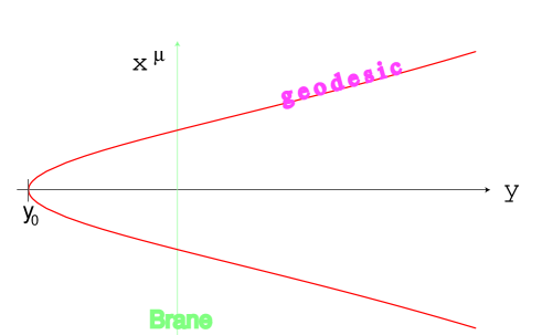
FIG. 1.: The bubbles once generated follow the geodesics of $AdS_{5}$. The AdS horizon is to the right.

The classical equations of motion of the brane can be readily derived, at least formally, from Eq. 1. Choosing coordinates $x^{\mu}$ on the brane and varying the position $X^{a}(x)$ of the brane, as well as the metric $G_{ab}$, in the action we find

$$\left(T^{\mu\nu}-\Lambda_{4}\,g^{\mu\nu}\right)\left(D_{\mu}D_{\nu}X^{c}+\Gamma^{c}_{ab}\partial_{\mu}X^{a}\partial_{\nu}X^{b}\right) = 0$$ (5)

$$\frac{1}{2\sqrt{-G}}\int d^{4}x\sqrt{-g(x)}\,\delta^{5}\left[z-X(x)\right]\,\left(T^{\mu\nu}-\Lambda_{4}g^{\mu\nu}\right)\partial_{\mu}X^{a}\partial_{\nu}X^{b} = 2M_{5}^{3}E^{ab}+{1\over 2}G^{ab},$$ (6)

where the first equation is satisfied on the brane (${\cal M}_{4}$) and the second everywhere on (${\cal M}_{5}$). The quantity $T^{\mu\nu}$ is the Standard Model energy-momentum tensor; $E^{ab}$ is the Einstein tensor calculated from the metric $G^{ab}$.

The first equation is a variant of the geodesic equation. The fact that it is invariant under a rescaling of all energy-momentum on the brane ($T^{\mu\nu}\rightarrow\lambda T^{\mu\nu}$, $\Lambda_{4}\rightarrow\lambda\Lambda_{4}$) is a reflection of the equivalence principle.

In Gaussian normal coordinates of the brane (i.e. $X^{y}(x)=0$ and $X^{\alpha}(x)=x^{\alpha}$) the second equation becomes

$$2M_{5}^{3}\,E^{ab}+{1\over 2}\Lambda_{5}G^{ab}=-{1\over 2}\delta(y)\left(T^{\mu\nu}-\Lambda_{4}g^{\mu\nu}\right).$$ (7)

This can be replaced by the vacuum equations for $y\neq 0$ and the Israel conditions [10]

$$\left(\lim_{y\to+0}-\lim_{y\to-0}\right)\,\left(K_{\mu\nu}-K\,g_{\mu\nu}\right)=-\frac{1}{4M_{5}^{3}}\left(T^{\mu\nu}-\Lambda_{4}g^{\mu\nu}\right).$$ (8)

Here $K_{\mu\nu}$ is the extrinsic curvature of the brane in the metric $G_{ab}$. The first equation becomes

$$\left(T^{\mu\nu}-\Lambda_{4}\,g^{\mu\nu}\right)K_{\mu\nu}=0.$$ (9)

This equation is ambiguous when no orbifold symmetry is imposed ($y\leftrightarrow-y$). A mathematically careful treatment of the variational problem in Eq. 1 reveals that the correct equation is found if $K_{\mu\nu}$ is replaced by the average of the two $K_{\mu\nu}$’s on the twe sides of the brane in Eq. 9.

In collider experiments we probe the regime where $T^{\mu\nu}$ is much smaller than $M_{5}$. We can see in Eqns. 7,8,9 that the $\frac{1}{M_{5}}\rightarrow 0$ limit must be taken. Then the metric $G^{ab}$ does not feel the effect of the brane any more and is exactly $AdS_{5}$, with the brane moving on this background, subject to only Eq. 9.

For a brane subject to orbifold boundary conditions, such fixed background prohibits all local perturbations. (This situation is similar to what happens on a flat background. Then the fixed surfaces of $Z_{2}$ isometries are only flat planes.) All processes involving bubble production (or production of the moduli for that matter) would be subleading in $\frac{energy}{M_{5}^{3}}$, suppressed by 15 orders of magnitude in our numerical example.

When no symmetry requirement is imposed, it is reasonable to write the equations of motion in flat 5-dimensional coordinates and specify the brane by one function (normalized so for future convenience):

$$X^{\mu}(x)=x^{\mu}\ \ \ \mbox{and}\ \ \ X^{5}=\Lambda_{4}^{-{1\over 2}}\Phi(x).$$ (10)

The induced metric in these coordinates becomes

$$g_{\mu\nu}=\eta_{\mu\nu}-\frac{1}{\Lambda_{4}}\partial_{\mu}\Phi\partial_{\nu}\Phi,\ \ \ \mbox{and also}\ \ \ \sqrt{-g}=\sqrt{1-\frac{1}{\Lambda_{4}}\eta^{\mu\nu}\partial_{\mu}\Phi\partial_{\nu}\Phi}.$$ (11)

The bulk part of the action is not varied any more but the brane part becomes

$$S=\int d^{4}x\,{\cal L}\ \ \ \mbox{with}\ \ \ {\cal L}(\Phi,\varphi)=\sqrt{-g}\,\left[{\cal L}_{SM}(g_{\mu\nu},\varphi)-\Lambda_{4}\right].$$ (12)

Expanding this Lagrangian in the $\Phi$ field we see that is is canonically normalized and is coupled derivatively to the energy momentum tensor of the SM fields. It is not hard to see that all the couplings, both to fermions and bosons, are dimension 8 and higher. For example, to a scalar we have a coupling $-{1\over 2\Lambda_{4}}\left(\partial_{\mu}\varphi\,\partial^{\alpha}\Phi\right)^{2}$. The symmetry $\Phi\rightarrow\Phi+const.$ corresponds to the translational invariance of the brane in the fifth direction. The $\Phi$ field is then the Goldstone boson corresponding to this symmetry.

Such a massless moduli field with $TeV$-scale couplings phenomenologically unacceptable. However, its Goldstone nature also implies that any explicit breaking of the fifth dimensional translations would give mass to the $\Phi$ field. In particular, so do mechanisms that stabilize interbrane separations in models with more than one brane [4]. In this letter we are only trying to establish the generic consequences of the $\overline{RS}$ idea and simply suppose that one way or another such mass has been generated.

Bubbles of brane matter can be considered as nontrivial topological configurations of the $\Phi$ fields. The classical equations of motion can be found in terms of the $\Phi$ field from the action in Eq. 12. Neglecting the SM fields,

$$\partial_{\mu}\frac{\eta^{\mu\nu}\partial_{\nu}\Phi}{\sqrt{1-{1\over\Lambda_{4}}\eta^{\alpha\beta}\partial_{\alpha}\Phi\partial_{\beta}\Phi}}=0.$$ (13)

For small field strength these equations describe harmonic oscillations of the brane.

Classically, these equations can be solved supposing spherical symmetry. The result is a collapsing bubble with time dependent radius $R(t)$, shown in Fig. 2,

$$t(R)=t_{0}\pm{\cal E}\int_{0}^{R/\cal E}\frac{du}{\sqrt{1-u^{6}}}.$$ (14)

The lifetime of the bubble equals $2.43\,{\cal E}$, where ${\cal E}^{3}=\frac{2E}{\pi^{2}\Lambda_{4}}$, with $E$ being the total energy contained in the bubble. This result is physically not surprising. When the SM field are thrown away, there is nothing to counteract the brane tension in pulling together the bubble.

Including the quantum fields on the surface of the bubble, the Casimir effect generates a vacuum energy density $\sim-\frac{\alpha}{R^{4}}$. The value and sign of the constant $\alpha\leq{\cal O}(1)$ depends on the topology of the bubble and the boundary conditions (periodic vs. antiperiodic), and is generically unknown. In a supersymmetric theory it may cancel [11] but even in the simple case of QED on $R\times S^{3}$ its sign is presently debated [12]. A positive value of $\alpha$ results in a stabilized bubble within a very short time $\sim{\cal E}$, with the Casimir energy roughly equal to the energy contained in the brane surface:

$$\frac{\alpha}{R^{4}}\times\frac{\pi^{2}}{2}R^{3}\approx\frac{\pi^{2}}{2}\Lambda_{4}R^{3},\ \ \ \mbox{i.e.}\ \ \ \Lambda_{4}R^{4}\approx\alpha$$ (15)

This fixes the internal energy contained in the bubble at the $TeV$ scale. We may take the point of view that bubbles with all sorts of topologies will be created but only those with a positive $\alpha$ survive.

The situation is analogous to perturbative bosonic string theory. In that case the classical string also collapses. In quantum language this is due to the presence of tachionic excitations. With more fields present on the worldsheet it is possible to arrange a situation when the tachionic modes decouple and the result is a spectrum with energy levels$\sim\Lambda_{2}^{1/2}$. In our case it is impossible to show without a detailed discussion of the field theory on the brane how such a mechanism explicitly works.

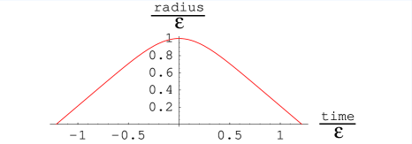
FIG. 2.: The classical collapse of a bubble. Here, ${\cal E}^{3}=\frac{2}{\pi^{2}}\frac{Energy}{\,\Lambda_{4}}$ determines the lifetime.

Now we turn to the discussion of bubble production. It should also be noted first that the quanta of the $\Phi$ field can be produced in pairs, due to the $\Phi\rightarrow-\Phi$ symmetry. This is a remnant of the $y\rightarrow-y$ symmetry of the Lagrangian which remains even if the metric solution is not required be symmetric. As a consequence, the probability to produce a bubble will be equal on the two sides. The difference shows up only at the scale of the $AdS$ curvature, well separated from the scale of bubble production.

In classical physics it is impossible to find the probability of producing a bubble in the linear approximation. The in state is vacuum and the $\Phi\leftrightarrow-\Phi$ symmetry prohibits any solution with $\Phi\neq 0$. Any solution arises as a consequence of the instability of the $\Phi=0$ solution. Even if we find such an unstable solution, the response is proportional to the input uncertainty of the $\Phi$ field strength (i.e. the brane position) which is not described correctly by classical physics.

In order to provide at least a crude quantum description of bubble generation we first model the SM process. For technical simplification we look at (3-dimensional) spherical symmetry. We take a state that contains one free particle localized in a region with radius $\rho$ that is allowed to flow apart in time to all directions. The wave function at $t=0$ is chosen to be $f(t=0,{\bf x})=\left(\frac{2}{\pi\rho^{2}}\right)^{3/4}e^{-\frac{r^{2}}{\rho^{2}}}$. The time evolution of this state is trivially found from the Fourier transform of the wave function which satisfies the Klein-Gordon equation (See Fig. 3.)

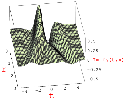
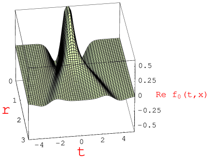
FIG. 3.: The time evolution of the wave function of the particle modeling the SM process. The m=0 case is shown.

The energy-momentum tensor is calculated next

$$T_{\mu\nu}=\left(\frac{\rho^{2}}{2\pi}\right)^{3/2}\int\int\frac{d^{3}{\bf k}\,d^{3}{\bf q}}{(2\pi)^{3}\sqrt{E_{\bf k}E_{\bf q}}}\left[k_{(\mu}q_{\nu)}+\eta_{\mu\nu}\frac{(k-q)^{2}}{4}\right]e^{-{\rho^{2}\over 4}\left({\bf k}^{2}+{\bf q}^{2}\right)}\cos\left[t(E_{\bf k}-E_{\bf q})-{\bf x}({\bf k}-{\bf q})\right].$$ (16)

In the next step we calculate the two particle state that is produced in the lowest order in ${1\over\Lambda_{4}}$ in perturbation theory. Note that although perturbation theory is not expected to be a good guide in the strong field regime, its predictions will provide the correct order of magnitude. The state at time $t$ is $|t\!>\ =|0\!>+\ |t\!>_{2}\$ with $|t\!>_{2}=\,\int\frac{d^{3}{\bf k}_{1}}{(2\pi)^{3/2}\sqrt{2E_{{\bf k}_{1}}}}\int\frac{d^{3}{\bf k}_{2}}{(2\pi)^{3/2}\sqrt{2E_{{\bf k}_{2}}}}c({\bf k}_{1},{\bf k}_{2})\hat{a}^{\dagger}_{{\bf k}_{1}}\hat{a}^{\dagger}_{{\bf k}_{1}}|0\!>$ and

$$c({\bf k}_{1},{\bf k}_{2})\,=\frac{-i}{2\Lambda_{4}}\int_{-\infty}^{t}dt^{\prime}\int d^{3}{\bf x}^{\prime}e^{i{\bf x}^{\prime}({\bf k}_{1}+{\bf k}_{2})}\left[T_{00}(t^{\prime},{\bf x}^{\prime})E_{{\bf k}_{1}}E_{{\bf k}_{2}}-T_{jl}(t^{\prime},{\bf x}^{\prime})k_{1}^{j}k_{2}^{l}\right].$$ (17)

where the free-field operator generates an elementary excitation of the $\Phi$ field.

The actual calculation of the probability to produce a topologically nontrivial field configuration requires exact knowledge of the fields on the brane. This is an unsolved problem beyond the scope of the present paper. Instead, we conjecture that a bubble of size $R$ will form whenever the energy density is larger than $\Lambda_{4}$ in a region of size $R$. If that happens, than with ${\cal O}(1)$ probability we will have a fluctuation of that compensates the force that is pulling together the brane. The intuitive classical image is that when the surface tension of the brane is compensated in a region, an instability develops and the brane will bulge out. Such a would-be bubble, if long enough compared to its size, will rather detach than be pulled back into our world.

Next we calculate the average energy density carried by the $\Phi$ field. We find

$$<t|{\cal H}(t,{\bf x})|t> = \int\frac{d^{3}{\bf q}_{1}}{(2\pi)^{3}2E_{\bf{q}_{1}}}\int\frac{d^{3}{\bf q}_{2}}{(2\pi)^{3}2E_{\bf{q}_{2}}}\left(E_{{\bf q}_{1}}q_{2}^{j}+E_{{\bf q}_{2}}q_{1}^{j}\right)$$ (19)

$$\times\left[c({\bf q}_{1},{\bf q}_{2})e^{i\,x\cdot(q_{1}+q_{2})}+\overline{c({\bf q}_{1},{\bf q}_{2})}e^{-i\,x\cdot(q_{1}+q_{2})}\right]+{\cal O}\left({1\over\Lambda_{4}^{2}}\right).$$

When we substitute Eqns. 16,17 into Eq. 19, we find a short-distance divergence. We regulate it by calculating the total amount of energy contained within radius $R$,

$${\cal E}(R) \equiv \int d^{3}{\bf x}<t|{\cal H}(t,{\bf x})|t>$$ (20)

$$= \frac{(\rho R)^{3}}{4\pi\Lambda_{4}}\int_{0}^{\infty}dpp^{4}e^{-\frac{\rho^{2}+R^{2}}{8}p^{2}}\int_{-\infty}^{\infty}dEe^{-itE}{\tilde{T}}^{E}(p)\ln(p-E+i0)+c.c.$$ (21)

with the $\Phi$ mass neglected, $E_{\pm}=|{\bf k}\pm\frac{1}{2}{\bf p}|$, and

$${\tilde{T}}^{E}(p) = {1\over 3}\int\frac{d^{3}{\bf k}}{\sqrt{E_{+}E_{-}}}e^{-\frac{\rho^{2}}{2}{\bf k}^{2}}\delta(E_{+}-E_{-}E)\left((E_{+}-E_{-})^{2}\ \left\{8{\bf k}^{2}-7\frac{(\bf k\cdot p)^{2}}{{\bf p}^{2}}-\frac{11}{4}(E_{+}-E_{-})^{2}+{\bf p}^{2}\right\}\right.$$ (23)

$$\left.-{\bf p}^{2}\ \left\{4{\bf k}^{2}-8\frac{(\bf k\cdot p)^{2}}{{\bf p}^{2}}-\frac{13}{4}(E_{+}-E_{-})^{2}+2{\bf p}^{2}\right\}\right).$$

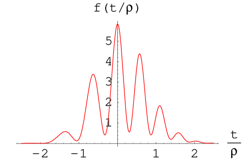
FIG. 4.: The energy density in the $\Phi$ field at $R=0$ as a function of time. The normalization is according to $\rho^{8}\Lambda_{4}\frac{{\cal E}(R)}{R^{3}}=f\left(\frac{t}{\rho}\right)$.

The resulting averaged energy density is shown in Fig. 4 in the case when $R<<\rho$. The production probability of a bubble is ${\cal O}(1)$ during time $R$ in a region of size $R$ wherever this energy density is in excess of $\Lambda_{4}$. Bubbles with size $R>>\rho$ can never be generated (With $\rho^{4}\leq\Lambda_{4}^{-1}$, the function $f$ is never $>>1$, and for large $R$ it is more suppressed.) The shape of the function in Fig. 4 tells us that to produce a bubble at all we need a minimum energy concentration $\rho^{4}\Lambda_{4}\leq\sqrt{f(0)}$. Once we achieve that, bubbles of all sizes $R\leq\rho$ will be produced with unit probability (this is a sign of that in the “hot” region of size $\rho$ an instability occurs.)

We see now that copious bubble production requires that the incoming particles be localized in a region $\rho\sim TeV^{-1}$. In a particle beam $\rho$ corresponds to the beam energy, $\rho\sim{1\over\sqrt{s}}$. The above calculation shows is that the threshold of bubble production is at $\sqrt{s}\sim\Lambda_{4}^{-1/4}$. This is so even for bubbles smaller than $R<\Lambda^{-1/4}$ whose production is possible only through tunneling. Even though the energy might be available in processes with $\sqrt{s}\sim\Lambda_{4}R^{3}<\Lambda_{4}^{-1/4}$, an energy density $\Lambda_{4}$ is not attained. Once the above threshold is reached, the production probability is ${\cal O}(1)$, the cross section is determined by the unitarity bound $\sigma\approx{1\over s}$.

The above rudimentary calculation of the expectation value of the energy density disregards energy fluctuations. Below the above threshold, with a small probability, it is possible that a large energy density fluctuation arises in a small region $R^{3}$ whose lifetime will be ${\cal O}(R)$. The probability of this is the same as producing a state of mass $M\sim 1/R$ (so it is localized in the bubble) and energy $E\sim{\Lambda_{4}R^{3}}$. This state represents the “hot region” mentioned in the previous discussion, and will decay into a bubble with branching ratio ${\cal O}(\frac{E^{4}}{\Lambda_{4}})\sim(\Lambda_{4}R^{4})^{3}$), due to the derivative couplings of the $\Phi$ field. This state is far off-shell and this introduces a suppression $(\frac{E}{{M}})^{4}\sim(\Lambda_{4}R^{4})^{4}$, so the cross section is $\sigma\sim\frac{(\Lambda_{4}R^{4})^{7}}{s}$. If we look at the largest bubbles that can be produced (they have the largest probability), $\sqrt{s}\sim E\sim\Lambda_{4}R^{3}$, we find $\sigma\sim\frac{1}{s}\,\left(\frac{\sqrt{s}}{\Lambda_{4}^{1/4}}\right)^{28/3}$.

We thus find that a high power of the energy suppresses the production of small bubbles. These bubbles in fact correspond to the massless states in string theory but in our case their mass (or existence) can be established only in a detailed model. If they exist, they should be visible in accelerator experiments somewhat below $\sqrt{s}<\Lambda_{4}^{1/4}.$ They would show up most easily if a charged particle gets trapped on the bubble.

Note that this effect does not induce (apparent) proton decay. Even though bubbles may be produced with a tiny probability at energies less than a $GeV$, no baryons can be trapped on them due to energy conservation. Ultimately, this is due to the fact that the bubble is not vanishing, only stopping to interact with our world.

Note that in the cosmological context at present time, even in supernova explosions the available energy for bubble production is too small. With a reasonable choice of $\sqrt{s}\sim 20MeV$ during the explosion, the average time a proton in a neutron star needs to form a bubble is (according to the above cross section) $\sim 10^{9}$ years, while the explosion lasts only tens of seconds.

In sum, the expected experimental signature includes (i) displaced vertices due to returning bubbles, (ii) missing energy and/or $p_{T}$, as well as missing baryon number, lepton number and electric charge as soon as the total energy reaches $\sqrt{s}\sim\Lambda_{4}^{1/4}$.

REFERENCES

- [1] L. Randall and R. Sundrum, “A large mass hierarchy from a small extra dimension,” Phys. Rev. Lett. 83, 3370 (1999) [hep-ph/9905221].
- [2] L. Randall and R. Sundrum, “An alternative to compactification,” Phys. Rev. Lett. 83 (1999) 4690 [hep-th/9906064].
- [3] J. Lykken and L. Randall, “The shape of gravity,” JHEP0006, 014 (2000) [hep-th/9908076].
- [4] W. D. Goldberger and M. B. Wise, “Phenomenology of a stabilized modulus,” Phys. Lett. B 475, 275 (2000) [hep-ph/9911457], “Modulus stabilization with bulk fields,” Phys. Rev. Lett. 83, 4922 (1999) [hep-ph/9907447].
- [5] D. J. Chung, L. Everett and H. Davoudiasl, “Experimental probes of the Randall-Sundrum infinite extra dimension,” hep-ph/0010103.
- [6] J. R. Bond et al., “CMB Analysis of Boomerang & Maxima & the Cosmic Parameters ”, In Proc. IAU Symposium 201 (PASP) [astro-ph/0011378]; S. Perlmutter et al., “Measurements of Omega and Lambda from 42 High-Redshift Supernovae,” Astrophys. J. 517, 565 (1999) [astro-ph/9812133]; A. E. Lange et al., “Cosmological parameters from the first results of BOOMERANG,” Phys. Rev. D 63, 042001 (2001) [astro-ph/0005004].
- [7] G. Dvali and G. Gabadadze, “Non-conservation of global charges in the brane universe and baryogenesis,” Phys. Lett. B 460, 47 (1999) [hep-ph/9904221].
- [8] F. C. Adams, G. L. Kane, M. Mbonye and M. J. Perry, hep-ph/0009154.
- [9] S. L. Dubovsky, V. A. Rubakov and P. G. Tinyakov, “Is the electric charge conserved in brane world?,” JHEP0008, 041 (2000) [hep-ph/0007179].
- [10] W. Israel, “Singular Hypersurfaces And Thin Shells In General Relativity,” Nuovo Cim. B44 S10, 1 (1966).
- [11] K. A. Milton, “Dimensional and dynamical aspects of the Casimir effect: Understanding the reality and significance of vacuum energy,” hep-th/0009173.
- [12] F. Ravndal, “Problems with the Casimir vacuum energy,” hep-ph/0009208.