Abstract

The production of baryons containing two charmed quarks $(\Xi^{*}_{cc}\mbox{ or }\Xi_{cc})$ in hadronic interactions at high energies and large transverse momenta is considered. It is supposed, that $\Xi_{cc}$-baryon is formed during a non-perturbative fragmentation of the $(cc)$-diquark, which was produced in the hard process of $c$-quark scattering from the colliding protons: $c+c\to(cc)+g$. It is shown that such mechanism enhances the expected doubly charmed baryon production cross section on Tevatron and LHC colliders approximately 2 times in contrast to predictions, obtained in the model of gluon - gluon production of $(cc)$-diquarks in the leading order of perturbative QCD.

1 Introduction

Doubly heavy baryons take the special place among baryons which contain heavy quarks. The existence of two heavy quarks causes the brightly expressed quark - diquark structure of the $\Xi_{cc}$ baryon, in a wave function which one’s the configuration with compact heavy $(QQ)$-diquark dominates. Regularity in a spectrum of mass of doubly heavy baryons appear in many respects to a similar case of mesons containing one heavy quark [1, 2, 3, 4]. Production mechanisms for $(QQq)$-baryons and $(Q\bar{q})$-mesons also have common features. At the first stage compact heavy $(QQ)$-diquark is formed, than it fragments in a final $(QQq)$-baryon, picking up a light quark. The calculations of production cross sections for doubly heavy baryons in $ep$- and $pp$-interactions were made recently as in the model of a hard fragmentation of a heavy quark in doubly heavy diquark [5, 6, 7] as within the framework of the model of precise calculation of cross section of a gluon – gluon fusion into doubly heavy diquarks and two heavy antiquarks in the leading order of the perturbation theory of QCD [8, 9, 10].

Mechanism of production of hadrons containing charmed quarks, based on consideration of hard parton subprocesses with one $c$-quark in an initial state, was discussed earlier in papers [11, 12, 13]. It was shown, that in the region of a large transferred momentum $(Q^{2}>>m_{c}^{2}$, where $m_{c}$ is charmed quark mass) the concept of a charm excitation in a hadron does not contradict parton model and allows to effectively take into account the contribution of the high orders of the perturbative QCD theory to the Born approximation. However, there is open problem of the ”double score”, which is determined by the fact that the part of the Born diagrams of birth of two heavy quarks in a gluon - gluon fusion can be interpreted, as the diagrams with charm excitation in one of initial protons. These diagrams give leading in $\alpha_{s}$ contribution in the $c$-quark perturbative, so-called point-like structure function (SF) of a proton. As to the non-perturbative contribution in $c-$quark SF of a proton [14] it does not depend from $Q^{2}$ and becomes very small at $Q^{2}>>m_{c}^{2}$.

For example, fig. 1 shows one of 36 Born diagrams, which have order $\alpha_{s}^{4}$, describing production of the $(cc)$-diquark in the gluon-gluon fusion subprocess. The experience in calculation of heavy quark production cross sections in a gluon - gluon fusion demonstrates that the contribution of the next order of the perturbative QCD in $\alpha_{s}$ can be comparable with the contribution of the Born diagrams. In the case of gluon – gluon production of the two pairs of heavy quarks there will be more than three hundred diagrams with additional gluon in the final state, which have order $\alpha_{s}^{5}$, and their direct calculation is now considered difficultly feasible.

2 Subprocess $c+c\to(cc)+g$

In this paper the model of $(cc)$-diquark production in proton - proton interactions, based on the mechanism of the charm excitation in a proton is considered. It is supposed, that the $(cc)$-diquark is formed during scattering of $c$-quarks from colliding protons with radiation of a hard gluon, i.e. in the parton subprocess:

$$c+c\to(cc)+g$$ (1)

The Feynman diagrams of the parton subprocess (1) are shown in fig. 2, where $q_{1}$ and $q_{2}$ are 4-momenta of the initial $c$-quarks, $k$ is 4-momentum of the final gluon, $p$ is 4-momentum of the diquark, which one is divided equally between the final $c$-quarks. The doubly heavy diquark is considered as bound state of two $c$-quarks in the antitriplet colour state and in the vector spin state. If $i$ and $j$ are colour indexes of initial quarks, and $m$ is colour index of a final diquark, the amplitude of production of the $(cc)$-diquark $M_{ijm}(c+c\to(cc)+g)$ is connected with the amplitude of production of two $c$-quarks with 4-momenta $p_{1}=p_{2}=\displaystyle{\frac{p}{2}}$ as follows:

$$M_{ijm}(c+c\to(cc)+g,p)=K_{0}\displaystyle\frac{\varepsilon^{nmk}}{\sqrt{2}}M_{ijnk}(c+c\to c+c+g,p_{1}=p_{2}=\displaystyle{\frac{p}{2}}),$$ (2)

where $K_{0}=\sqrt{\displaystyle{\frac{2}{m_{cc}}}}\Psi_{cc}(0)$, $m_{cc}=2m_{c}$ is the diquark mass, $\Psi_{cc}(0)$ is the diquark wave function in zero point, $\displaystyle{\frac{\varepsilon^{nmk}}{\sqrt{2}}}$ is the colour part of a diquark wave function. Considering spin degrees of freedom of $c-$quarks and $(cc)$-diquark, we have following conformity between amplitudes of birth of free quarks and a diquark with fixed spin projections (without colour indexes and common factor $K_{0}$):

$$M(c+c\to(cc)+g,s_{z}=+1) \sim M(c+c\to c+c+g,s_{1z}=+1/2,s_{2z}=+1/2)$$ (3)

$$M(c+c\to(cc)+g,s_{z}=-1) \sim M(c+c\to c+c+g,s_{1}z=-\frac{1}{2},s_{2z}=-\frac{1}{2})$$ (4)

$$M(c+c\to(cc)+g,s_{z}=0) \sim \frac{1}{\sqrt{2}}\Biggl{[}M(c+c\to c+c+g,s_{1}z=+\frac{1}{2},s_{2z}=-\frac{1}{2})+$$ (5)

$$+ M(c+c\to c+c+g,s_{1z}=-\frac{1}{2},s_{2z}=+\frac{1}{2})\Biggr{]}.$$

Because the wave function of the $(cc)$-diquark is antisymmetric on colour index and symmetric on remaining indexes, the production of the scalar $(cc)$-diquark is forbidden, i.e.

$$M(c+c\to c+c+g,s_{1z}=+\frac{1}{2},s_{2z}=-\frac{1}{2})-M(c+c\to c+c+g,s_{1z}=-\frac{1}{2},s_{2z}=+\frac{1}{2})=0.$$ (6)

Amplitudes adequate to the diagrams in fig. 2, where the final c-quarks are in the arbitrary spin states, are written out below, without the colour factors and the common factor $K_{0}$:

$$M_{1}=g_{s}^{3}\varepsilon_{\mu}(k)\bar{U}(p_{1})\gamma^{\mu}(\hat{p}_{1}+\hat{k}+m_{c})\gamma^{\nu}U(q_{1})\bar{U}(p_{2})\gamma_{\nu}U(q_{2})/{((p_{1}+k)^{2}-m_{c}^{2})(p_{2}-q_{2})^{2}}$$ (7)

$$M_{2}=g_{s}^{3}\varepsilon_{\mu}(k)\bar{U}(p_{1})\gamma^{\nu}U(q_{1})\bar{U}(p_{2})\gamma^{\mu}(\hat{p}_{2}+\hat{k}+m_{c})\gamma_{\nu}U(q_{2})/((p_{2}+k)^{2}-m_{c}^{2})(q_{1}-p_{1})^{2}$$ (8)

$$M_{3}=g_{s}^{3}\varepsilon_{\mu}(k)\bar{U}(p_{1})\gamma^{\nu}(\hat{q}_{1}-\hat{k}+m_{c})\gamma^{\mu}U(q_{1})\bar{U}(p_{2})\gamma_{\nu}U(q_{2})/((q_{1}-k)^{2}-m_{c}^{2})(p_{2}-q_{2})^{2}$$ (9)

$$M_{4}=g_{s}^{3}\varepsilon_{\mu}(k)\bar{U}(p_{1})\gamma^{\nu}U(q_{1})\bar{U}(p_{2})\gamma^{\nu}(\hat{q}_{2}-\hat{k}+m_{c})\gamma_{\mu}U(q_{2})/((q_{2}-k)^{2}-m_{c}^{2})(q_{1}-p_{1})^{2}$$ (10)

$$M_{5}=g_{s}^{3}\varepsilon_{\mu}(k)\bar{U}(p_{1})\gamma^{\nu}U(q_{1})\bar{U}(p_{2})\gamma^{\lambda}U(q_{2})G_{\lambda\mu\nu}(p_{2}-q_{2},k,p_{1}-q_{1})/{(q_{1}-p_{1})^{2}(p_{2}-q_{2})^{2}}$$ (11)

where $g_{s}=\sqrt{4\pi\alpha_{s}}$, $\alpha_{s}$ is strong coupling constant, $G_{\lambda\mu\nu}(p,k,q)=(p-k)_{\nu}g_{\lambda\mu}+(k-q)_{\lambda}g_{\nu\mu}+(q-p)_{\mu}g_{\nu\lambda}$. Let’s remark, that the amplitudes $M_{6}-M_{10}$ are received by replacement of the initial quarks momenta $q_{1}\leftrightarrow q_{2}$ in the amplitudes $M_{1}-M_{5}$ ans are taken with a minus sign, that allows for the antisymmetrization of the initial state of two identical $c$-quarks. The corresponding colour factors are presented by the following expressions:

$$C_{1}=\frac{\varepsilon^{nmk}}{\sqrt{2}}(T^{c}_{nl}T^{b}_{li})(T^{b}_{kj}),\quad C_{6}=\frac{\varepsilon^{nmk}}{\sqrt{2}}(T^{c}_{nl}T^{b}_{lj})(T^{b}_{ki}),$$

$$C_{2}=\frac{\varepsilon^{nmk}}{\sqrt{2}}(T^{b}_{ni})(T^{c}_{kl}T^{b}_{lj}),\quad C_{7}=\frac{\varepsilon^{nmk}}{\sqrt{2}}(T^{c}_{nj})(T^{c}_{kl}T^{b}_{li}),$$

$$C_{3}=\frac{\varepsilon^{nmk}}{\sqrt{2}}(T^{b}_{nl}T^{c}_{li})(T^{b}_{kj}),\quad C_{8}=\frac{\varepsilon^{nmk}}{\sqrt{2}}(T^{b}_{nl}T^{c}_{lj})(T^{b}_{ki}),$$ (12)

$$C_{4}=\frac{\varepsilon^{nmk}}{\sqrt{2}}(T^{b}_{ni})(T^{b}_{kl}T^{c}_{lj}),\quad C_{8}=\frac{\varepsilon^{nmk}}{\sqrt{2}}(T^{b}_{nj})(T^{b}_{kl}T^{c}_{li}),$$

$$C_{5}=\frac{i\varepsilon^{nmk}}{\sqrt{2}}(T^{b}_{ni})(T^{a}_{kj})f^{bac},\quad C_{10}=\frac{i\varepsilon^{nmk}}{\sqrt{2}}(T^{b}_{nj})(T^{a}_{ki})f^{bac}.$$

Using known property of a completely antisymmetric tensor of the third rank

$$\varepsilon_{n^{\prime}mk^{\prime}}\varepsilon^{nmk}=\delta^{n}_{n^{\prime}}\delta^{k}_{k^{\prime}}-\delta^{k}_{n^{\prime}}\delta^{n}_{k^{\prime}},$$

it is easy to find products of the colour factors $\displaystyle C_{i,j}=\sum_{color}C_{i}C^{*}_{j}$, which ones are presented in the Appendix A.

The method of the calculation of a production amplitude of a bound nonrelativistic state of quarks in the fixed spin state is based on a formalism of the projection operator [15]. Using properties of the charge conjugation matrix $C=i\gamma_{2}\gamma_{0}$, we can link a scattering amplitude of a quark on a quark with a scattering amplitude of an antiquark on a quark, for example:

$$M_{1}=g_{s}^{3}\varepsilon_{\mu}(k)\bar{U}(p_{1})\gamma^{\mu}(\hat{p}_{1}+\hat{k}+m_{c})\gamma^{\nu}U(q_{1})\bar{U}(p_{2})\gamma_{\nu}U(q_{2})/((p_{1}+k)^{2}-m_{c}^{2})(p_{2}-q_{2})^{2}=$$

$$=g_{s}^{3}\varepsilon_{\mu}(k)\bar{V}(q_{1})\gamma^{\nu}(-\hat{p}_{1}-\hat{k}+m_{c})\gamma^{\mu}V(p_{1})\bar{U}(p_{2})\gamma_{\nu}U(q_{2})/((p_{1}+k)^{2}-m_{c}^{2})(p_{2}-q_{2})^{2}.$$ (13)

As it may be shown, at $\displaystyle{p_{1}=p_{2}=\frac{p}{2}}$ one has:

$$V(p_{1},s_{1z}=-\frac{1}{2})\bar{U}(p_{2},s_{2z}=+\frac{1}{2})\sim\hat{\varepsilon}(p,s_{z}=+1)(\hat{p}+m_{cc}),$$

$$V(p_{1},s_{1z}=+\frac{1}{2})\bar{U}(p_{2},s_{2z}=-\frac{1}{2})\sim\hat{\varepsilon}(p,s_{z}=-1)(\hat{p}+m_{cc}),$$ (14)

$$\frac{1}{\sqrt{2}}\Bigl{[}V(p_{1},s_{1z}=-\frac{1}{2})\bar{U}(p_{2},s_{2z}=+\frac{1}{2})+$$

$$+V(p_{1},s_{1z}=+\frac{1}{2})\bar{U}(p_{2},s_{2z}=-\frac{1}{2})\Bigr{]}\sim\hat{\varepsilon}(p,s_{z}=0)(\hat{p}+m_{cc}),$$

where $\varepsilon^{\mu}(p)$ – is polarization 4-vector of a spin-1 particle. After following effective replacements

$$V(p_{1})\bar{U}(p_{2})\rightarrow\hat{\varepsilon}(p)(\hat{p}+m_{cc})\mbox{ and }K_{0}\rightarrow K,$$ (15)

where $p_{1}=p_{2}=p/2$ and $\displaystyle K=\frac{\Psi(0)}{2\sqrt{m_{cc}}}$, amplitudes $M_{i}$, with corresponding colour factors $C_{i}$, describe production of the $(cc)$-diquark with fixed polarization. The square of the module of amplitude of $(cc)$-diquark production after average on spin and colour degrees of freedom is given by the following expression:

$$\overline{|{\cal M}|^{2}}=\displaystyle{\frac{1}{36}}K^{2}\sum_{i,j=1}^{10}\sum_{spin}M_{i}(p_{1},p_{2})M_{j}^{*}(p_{1},p_{2})C_{i,j},$$ (16)

where in the amplitudes $M_{i}$ we have put $p_{1}=p_{2}=\displaystyle{\frac{p}{2}}$. The summation on vector diquark polarizations in the square of the amplitude of the process (1) was done using the standard formula:

$$\sum_{spin}\varepsilon^{\mu}(p)\varepsilon^{*\nu}(p)=-g^{\mu\nu}+\displaystyle{\frac{p^{\mu}p^{\nu}}{m_{cc}^{2}}}.$$ (17)

The calculation of the value $F=\displaystyle{\sum_{i,j}^{10}\sum_{spin}M_{i}M_{j}^{*}C_{i,j}}$ have been executed using the package of an analytical calculations FeynCalc [16]. The answer is shown in the Appendix B, as a function of standard Mandelstam variables $\hat{s}$ and $\hat{t}$.

3 RESULTS OF CALCULATIONS

In the parton model the cross section of a $(cc)$-diquark production in $pp$-interactions is represented as follows:

$$\displaystyle{\frac{d\sigma}{dp_{\bot}}}(pp\to(cc)+X) = p_{\bot}\int^{y_{max}}_{y_{min}}dy\int^{1}_{x_{1min}}dx_{1}C_{p}(x_{1},Q^{2})C_{p}(x_{2},Q^{2})\times$$ (18)

$$\times\displaystyle{\frac{\overline{|{\cal M}|^{2}}}{16\pi(s(s-m_{cc}^{2}))^{1/2}}\times\frac{1}{x_{1}s-\sqrt{s}m_{\bot}e^{y}}},$$

where

$$x_{2}=\displaystyle{\frac{x_{1}\sqrt{s}m_{\bot}e^{-y}-\frac{3}{2}m_{cc}^{2}}{x_{1}s-\sqrt{s}m_{\bot}e^{y}}},$$

$$x_{1min}=\displaystyle{\frac{\sqrt{s}m_{\bot}e^{y}-\frac{3}{2}m_{cc}^{2}}{s-\sqrt{s}m_{\bot}e^{-y}}},$$

$C_{p}(x,Q^{2})$ is the $c$-quark distribution function in a proton at $Q^{2}=m_{\bot}^{2}=m_{cc}^{2}+p_{\bot}^{2}$, $p_{\bot}$ is the diquark transverse momentum, $y$ is the rapidity of the diquark in c.m.f. of colliding protons,

$$\hat{s}=(q_{1}+q_{2})^{2}=x_{1}x_{2}s+\displaystyle{\frac{m_{cc}^{2}}{2}},$$

$$\hat{t}=(q_{1}-p)^{2}=\displaystyle{\frac{3}{2}m_{cc}^{2}}-x_{1}\sqrt{s}m_{\bot}e^{-y},$$ (19)

$$\hat{u}=(q_{2}-p)^{2}=\displaystyle{\frac{3}{2}m_{cc}^{2}}-x_{2}\sqrt{s}m_{\bot}e^{y}.$$

It is supposed that spin-$\frac{1}{2}$ and spin-$\frac{3}{2}$ $\Xi_{cc}-$baryons relative yield is $1:2$ as it is predicted by the simple counting rule for the spin states. The production cross section of $\Xi_{cc}$-baryons plus $\Xi_{cc}^{*}-$baryons in our approach is connected with the production cross section of $(cc)$-diquark within the framework of a model of a non-perturbative fragmentation as follows:

$${\frac{d\sigma}{dp_{\bot}}(pp\to\Xi_{cc}+X)=\int^{1}_{0}\frac{dz}{z}\frac{d\sigma}{dp^{\prime}_{\bot}}(pp\to(cc)X,p^{\prime}_{\bot}=\frac{p_{\bot}}{z})D_{(cc)\to\Xi_{cc}}(z,Q^{2})},$$ (20)

where $D_{(cc)\to\Xi_{cc}}(z,Q^{2})$ is the phenomenological function of a fragmentation, normalized approximately on unity, as a total probability of transition $(cc)$-diquark in final doubly charmed baryon. At $Q^{2}=m_{cc}^{2}$ the fragmentation function is selected in the standard form [17]:

$$D_{(cc)\to\Xi_{cc}}(z,Q^{2})=\displaystyle{\frac{D_{0}}{\displaystyle{z(m_{cc}^{2}-\frac{m_{\Xi}^{2}}{z}-\frac{m_{q}^{2}}{1-z})^{2}}}},$$ (21)

where $m_{\Xi}=m_{cc}+m_{q}$ is the $\Xi_{cc}$-baryon mass, $m_{q}$ is the light quark mass, $D_{0}$ the is rate-fixing constant. The fragmentation function for $Q^{2}>Q^{2}_{0}$ can be determined by the solving the DGLAP evolution equation [18]. Following to paper [10], at numerical calculations we have used following values of parameters: $m_{cc}=3.4$ GeV, $\alpha_{s}=0.2$, $|\Psi_{cc}(0)|^{2}=0.03$ GeV³, $m_{q}=0.3$ GeV. For a $c-$quark distribution function in a proton $C_{p}(x,Q^{2})$ the parametrization CTEQ5 [19] was used. In figures 3 and 4 at $\sqrt{s}=1.8$ TeV and $\sqrt{s}=14$ TeV, accordingly, the curves show results of our calculations of $p_{\bot}$-spectra $(|y|<1)$ of $\Xi_{cc}$-baryons, the stars show results of the calculations from paper [10], adequate to the contribution of the gluon-gluon fusion production of $\Xi_{cc}$-baryons in a Born approximation. Thus, our calculations demonstrate, that the observed production cross section of $\Xi_{cc}$-baryons on colliders Tevatron and LHC can be approximately 2 times more at the expense of the contribution of the parton subprocess $c+c\to(cc)+g$, than it was predicted earlier in the papers [8, 10].

The authors thank S.P. Baranov, V.V. Kiselev and A.K. Likhoded for useful discussions. The work is executed at support of the Program ”Universities of Russia – Basic Researches” (Project 02.01.03).

Appendix A

$C_{1,1}=\frac{7}{9}$,	$C_{2,3}=\frac{10}{9}$,	$C_{3,6}=-\frac{10}{9}$,	$C_{4,10}=-2$,	$C_{6,10}=1$
$C_{1,2}=\frac{1}{9}$,	$C_{2,4}=-\frac{2}{9}$,	$C_{3,7}=\frac{2}{9}$,	$C_{5,5}=3$,	$C_{7,7}=\frac{7}{9}$
$C_{1,3}=-\frac{2}{9}$,	$C_{2,5}=1$,	$C_{3,8}=\frac{8}{9}$,	$C_{5,6}=-1$,	$C_{7,8}=\frac{10}{9}$
$C_{1,4}=\frac{10}{9}$,	$C_{2,6}=-\frac{7}{9}$,	$C_{3,9}=-\frac{16}{9}$,	$C_{5,7}=1$,	$C_{7,9}=-\frac{2}{9}$
$C_{1,5}=-1$,	$C_{2,7}=-\frac{1}{9}$,	$C_{3,10}=2$,	$C_{5,8}=2$,	$C_{7,10}=1$
$C_{1,6}=-\frac{1}{9}$,	$C_{2,8}=\frac{2}{9}$,	$C_{4,4}=\frac{16}{9}$,	$C_{5,9}=-2$,	$C_{8,8}=\frac{16}{9}$
$C_{1,7}=-\frac{7}{9}$,	$C_{2,9}=-\frac{10}{9}$,	$C_{4,5}=-2$,	$C_{5,10}=3$,	$C_{8,9}=-\frac{8}{9}$
$C_{1,8}=-\frac{10}{9}$,	$C_{2,10}=1$,	$C_{4,6}=\frac{2}{9}$,	$C_{6,6}=\frac{7}{9}$,	$C_{8,10}=2$
$C_{1,9}=\frac{2}{9}$,	$C_{3,3}=\frac{16}{9}$,	$C_{4,7}=-\frac{10}{9}$,	$C_{6,7}=\frac{1}{9}$,	$C_{9,9}=\frac{16}{9}$
$C_{1,10}=-1$,	$C_{3,4}=-\frac{8}{9}$,	$C_{4,8}=-\frac{16}{9}$,	$C_{6,8}=-\frac{2}{9}$,	$C_{9,10}=-2$
$C_{2,2}=\frac{7}{9}$,	$C_{3,5}=2$,	$C_{4,9}=\frac{8}{9}$,	$C_{6,9}=\frac{10}{9}$,	$C_{10,10}=3$

Appendix B

$$F=-(4\pi\alpha_{s})^{3}\frac{512F_{N}}{9F_{D}}$$ (22)

$$F_{N} = 26361\,M^{18}-6\,M^{16}\,\Bigl{(}20513\,s+67472\,t\Bigr{)}+$$ (23)

$$+16\,M^{14}\,\Bigl{(}14621\,s^{2}+100076\,s\,t-86020\,t^{2}\Bigr{)}-$$

$$-16\,M^{12}\,\Bigl{(}14873\,s^{3}+122408\,s^{2}\,t-657280\,s\,t^{2}-382560\,t^{3}\Bigr{)}+$$

$$+64\,M^{10}\,\Bigl{(}2101\,s^{4}-658\,s^{3}\,t-509652\,s^{2}\,t^{2}-468736\,s\,t^{3}-170408\,t^{4}\Bigr{)}+$$

$$+65536\,s\,t^{2}\,{\Bigl{(}s+t\Bigr{)}}^{2}\,\Bigl{(}9\,s^{4}+11\,s^{3}\,t+13\,s^{2}\,t^{2}+4\,s\,t^{3}+2\,t^{4}\ \Bigr{)}-$$

$$-256\,M^{8}\,\Bigl{(}120\,s^{5}-8749\,s^{4}\,t-201737\,s^{3}\,t^{2}-$$

$$-255896\,s^{2}\,t^{3}-149332\,s\,t^{4}-44640\,t^{5}\Bigr{)}-$$

$$-1024\,M^{6}\,\Bigl{(}7\,s^{6}+2180\,s^{5}\,t+44390\,s^{4}\,t^{2}+$$

$$+74060\,s^{3}\,t^{3}+57876\,s^{2}\,t^{4}+28176\,s\,t^{5}+7184\,t^{6}\ \Bigr{)}-$$

$$-16384\,M^{2}\,t\,\Bigl{(}10\,s^{7}+353\,s^{6}\,t+924\,s^{5}\,t^{2}+$$

$$+1151\,s^{4}\,t^{3}+898\,s^{3}\,t^{4}+460\,s^{2}\,t^{5}+160\,s\,t^{6}+28\,t^{7}\Bigr{)}+$$

$$+4096\,M^{4}\,\Bigl{(}s^{7}+235\,s^{6}\,t+5484\,s^{5}\,t^{2}+11610\,s^{4}\,t^{3}+$$

$$+11609\,s^{3}\,t^{4}+7368\,s^{2}\,t^{5}+3056\,s\,t^{6}+672\,t^{7}\Bigr{)}\$$

$$F_{D}={\Bigl{(}M^{2}-s\Bigr{)}}^{2}\,{\Bigl{(}M^{2}-4\,t\Bigr{)}}^{4}\,{\Bigl{(}5\,M^{2}-4\,\Bigl{(}s+t\Bigr{)}\Bigr{)}^{4}}$$ (24)

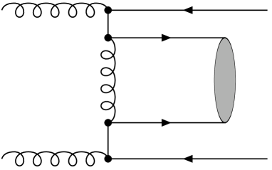
Figure 1:

One of the Born diagrams used for description subprocess $g+g\to(cc)+\bar{c}+\bar{c}$.

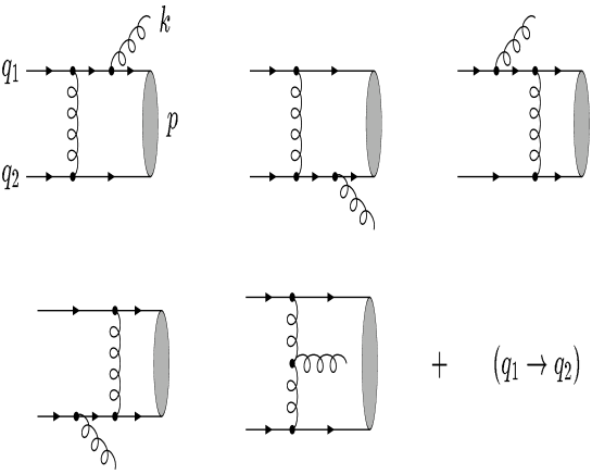
Figure 2:

Diagrams used for description subprocess $c+c\to(cc)+g$.

Figure 3:

Cross section of $\Xi_{cc}$-baryon production at $\sqrt{s}=1.8$ TeV and $|y|<1$. Stars (*) show the results of calculation from paper [10], curve is our result obtained in the model of a charm excitation in colliding protons.

Figure 4:

Cross section of $\Xi_{cc}$-baryon production at $\sqrt{s}=14$ TeV and $|y|<1$. Stars (*) show the results of calculation from paper [10], curve is our result obtained in the model of a charm excitation in colliding protons.

References

• [1] S.Fleck and J.Richard, Prog.Theor.Phys.82, 760 (1989).
• [2] E.Bagan et al., Z.Phys. C64, 57 (1994).
• [3] V.V.Kiselev et al., Phys.Lett. B332, 411 (1994).
• [4] D.Ebert et al., Z.Phys.C76, 111 (1997).
• [5] A.F.Falk et al., Phys.Rev. D49, 555 (1994).
• [6] A.P.Martynenko and V.A.Saleev, Phys.Lett. B385, 297 (1996).
• [7] V.A. Saleev, Phys.Lett., B426, 384 (1998).
• [8] A.V.Berezhnoy et al., Yad.Fiz. 59, 909 (1996).
• [9] S.P.Baranov, Phys.Rev. D54, 3228 (1996).
• [10] A.V.Berezhnoy et al., Phys.Rev. D57, 4385 (1998).
• [11] V.A.Saleev, Mod.Phys.Lett. A9, 1083 (1994).
• [12] A.P.Martynenko and V.A.Saleev, Phys.Lett. B343, 381 (1995).
• [13] S.P.Baranov, Phys.Rev. D56, 3046 (1997).
• [14] S.J.Brodsky and R.Vogt, Nucl.Phys. 478, 311 (1996).
• [15] B. Guberina et al., Nucl. Phys., B174, 317 (1980).
• [16] R.Mertig, The FeynCalc Book, Mertig Research and Consulting, 1999.
• [17] C. Peterson, Phys.Rev. D27, 105 (1983).
• [18] V.N. Gribov and L.N. Lipatov, Sov.J.Nucl.Phys. 15, 438 (1972); Yu.A. Dokshitser, Sov.Phys.JETP, 46, 641 (1977); G. Altarelli and G.Parisi, Nucl.Phys., B126, 298 (1977).
• [19] H.L. Lai et al., (CTEQ Coll.), Preprint hep-ph 9903282.