Abstract

We perform an oscillation parameter-independent analysis of solar neutrino flux measurements from which we predict the charged-current rate at SNO relative to Standard Solar Model to be $R_{\rm SNO}^{CC}=0.35^{+0.16}_{-0.09}(0.46^{+0.13}_{-0.11})$ for oscillations to active (sterile) neutrinos. By alternately considering the ⁸B flux normalization fixed and free, we find that the flux measured by Super-Kamiokande (SK) not being a result of oscillations is strongly disfavored for oscillations to active neutrinos. SNO will determine the best-fit value of the ⁸B flux normalization $\beta$ (equal to the neutral-current rate), without recourse to neutral-current measurements, from the derived relation $\beta=R_{\rm SNO}^{NC}=5.85R_{\rm SK}-4.85R_{\rm SNO}^{CC}$. Using a simple parameterization of the fraction of high, intermediate, and low energy solar neutrinos starting above resonance, we reproduce the results of global analyses to good accuracy; we find that the LMA solution with a normal mass hierarchy is clearly favored. With $\beta$ free, our analysis for oscillations to active neutrinos gives $R_{\rm SNO}^{NC}=\beta=1.34\pm 0.34$, which corresponds to $R_{\rm SNO}^{CC}=0.28\pm 0.07$.

I Introduction

Solar neutrino experiments measure an energy-dependent flux suppression  [1, 2, 3, 4, 5] relative to the Standard Solar Model (SSM) [6]. This situation has existed for thirty years and every new solar neutrino experiment has confirmed the flux-deficit. The best motivated explanation of this solar neutrino puzzle is that neutrinos are massive and undergo oscillations. The energy dependence of the flux suppression singles out very specific regions in the space of parameters that govern the frequency and amplitude of neutrino oscillations. The solar-neutrino flux deficit can be accounted for by oscillations of electron neutrinos to mu and/or tau neutrinos or to sterile neutrinos that do not interact weakly. In the two-neutrino oscillation framework, oscillations into sterile neutrinos are excluded at the 95% C. L. [7] by a comparison of the day and night spectra at Super-Kamiokande (Super–K) and the results of a global flux analysis; hence the favored explanation is $\nu_{e}\rightarrow\nu_{\mu}/\nu_{\tau}$ oscillations. For such oscillations, there are three regions (LMA, SMA and LOW) in the mass-squared difference $\delta m^{2}$ and vacuum amplitude $\sin^{2}2\theta$ parameters. These solutions involve effects from coherent $\nu_{e}$ scattering from matter [9] in the Earth and the Sun. Of these regions, the SMA region is disfavored at the 95% C. L. because of the observed flat energy spectrum and imperceptible day/night effect at Super–K [7]. For this reason we drop further consideration of the SMA region. A fourth region, the VAC or Just-So solution, which is largely independent of matter effects, is also excluded at the 95% C. L. by the same considerations that disfavor the SMA solution. Thus, we are left with the LMA and LOW regions, both of which have large mixing. With a large measure of certainty the KamLAND [10] experiment will exclude or confirm the LMA region as a solution to the solar neutrino anomaly [11, 12]. The SNO experiment [13] will be crucial in validating the above conclusions from the Super–K experiment [14, 15].

In this Letter we first perform a simple neutrino oscillation-independent analysis (with SSM fluxes) of the solar neutrino data using the total rates at the ³⁷Cl [1] and ⁷¹Ga [2, 3, 4] experiments and Super–K, following the procedure proposed in Ref. [16]. We make predictions for the charged-current (CC) rate at the SNO experiment. Allowing the ⁸B flux normalization to be free, we derive a relation for the neutral-current (NC) rate at SNO in terms of the CC rate at SNO in a model-independent way. Our analysis is suited to the LMA and LOW solutions for which the oscillations in matter are mainly adiabatic. We find the relative flux suppression of the high, intermediate, and low energy solar neutrinos, compared to the SSM, and how these suppressions depend on the normalization of the solar ⁸B neutrino flux. We then apply our analysis to the LMA and LOW solutions and approximately reproduce the results of more comprehensive fits. Finally, we predict the CC and NC rates at SNO for the ⁸B flux normalization obtained by imposing adiabatic constraints.

II Model-Independent Analysis

Following the procedure of Ref. [16], we divide the solar neutrino spectra into three parts: high energy (consisting of ⁸B and $hep$ neutrinos), intermediate energy (⁷Be, $pep$, ¹⁵O, and ¹³N), and low energy ($pp$). For each class of solar neutrino experiment the fractional contribution without oscillations to the expected rate from each part of the spectrum can be calculated in the SSM (see Table I). If $R$ is the measured rate divided by the SSM prediction for a given experiment, then with oscillations,

$$R_{\rm Cl} = 0.764P_{H}+0.236P_{I}\,,$$ (1)

$$R_{\rm Ga} = 0.096P_{H}+0.359P_{I}+0.545P_{L}\,,$$ (2)

where $P_{H}$, $P_{I}$, and $P_{L}$ are the average survival probabilities for the high, intermediate, and low energy solar neutrinos. In Eqs. (1) and (2) we assume that each probability remains the same from experiment to experiment, which is justified since the differential event rate without oscillations for each part of the spectrum has approximately the same shape for all experiments [16].

The SNO experiment detects neutrinos with energy above 5 MeV primarily via the reaction $\nu_{e}+d\rightarrow p+p+e^{-}$; the predicted CC rate is

$$R_{\rm SNO}^{CC}=P_{H}\,.$$ (3)

TABLE I.: Fractional contribution of the high, intermediate and low energy neutrinos to the ³⁷Cl, ⁷¹Ga and Super–K signals without oscillations. The last column gives the normalization uncertainty for each part of the spectrum.

				Super–K	Normalization
		37Cl	71Ga	SNO	Uncertainty
High	8B, $hep$	0.764	0.096	1.000	18.0%
Intermediate	7Be, $pep$, 15O, 13N	0.236	0.359	0.000	11.6%
Low	$pp$	0.000	0.545	0.000	1.0%

The $R$ formula for Super–K is different from SNO, even though both experiments are sensitive to only the high energy neutrinos, because Super–K detects active neutrinos by elastic scattering, $\nu_{x}+e^{-}\rightarrow\nu_{x}^{\prime}+e^{-}$ ($\nu_{x}$ denotes any of the active flavors), and that has neutral-current contributions. Using the NC/CC cross section ratio of 0.171 (for $x_{W}=0.225$), we have

$$R_{\rm SK} = 0.829P_{H}+0.171\ \ \ \,{\rm~{}(active)}\,,$$ (4)

$$= P_{H}\ \ \ \ \ \ \ \ \ \ \ \ \ \ \ \ \ \ \ \ \ {\rm~{}(sterile)}\,.$$ (5)

The solar neutrino data are summarized in Table II. Since there are three probability unknowns and three data points, there is an unique solution for the $P_{j}$. The Super–K rate depends only on the high energy neutrinos, so $P_{H}$ is directly determined by $R_{\rm SK}$. Then since $R_{\rm Cl}$ depends only on $P_{I}$ and $P_{H}$, the value of $P_{I}$ may be determined from $R_{\rm Cl}$. Finally, $P_{L}$ may be determined from $R_{\rm Ga}$. The best-fit values to the data in Table II are

$$P_{H} = 0.347\,,\ P_{I}=0.303\,,\ \ \ P_{L}=0.811\ \ \,{\rm~{}(active)}\,.$$ (6)

$$P_{H} = 0.459\,,\ P_{I}=-0.058\,,\ P_{L}=1.029\ \ {\rm~{}(sterile)}\,,$$ (7)

The sterile solution lies somewhat outside of, although close to, the physical region.

$$\begin{array}[]{lc|cc}\rm{Experiment}&&&\rm{data/SSM}\\ \hline\cr^{37}\rm{Cl}&&&0.337\pm 0.030\\ ^{71}\rm{Ga}&&&0.584\pm 0.039\\ {\rm{Super\!-\!K}}&&&0.459\pm 0.017\end{array}$$ (12)

TABLE II.: Solar neutrino data [1, 2, 3, 4, 5] expressed as the ratio $R=$ data/SSM, including the experimental uncertainties. The ⁷¹Ga number combines the results of the GALLEX, SAGE, and GNO experiments.

To determine the allowed regions in probability space, we include the experimental uncertainties in the measured values and the theoretical uncertainties of the high, intermediate, and low energy neutrino fluxes in the SSM (see Table I). We use the following expression for $\chi^{2}$:

$$\chi^{2}=\sum_{i}{(R_{i}-R_{i}^{th})^{2}\over\delta R_{i}^{2}+a_{i}^{2}P_{H}^{2}\delta_{H}^{2}+b_{i}^{2}P_{I}^{2}\delta_{I}^{2}+c_{i}^{2}P_{L}^{2}\delta_{L}^{2}}\,.$$ (13)

Here $i$ runs over the three types of experiments (³⁷Cl, ⁷¹Ga, and Super–K), $R_{i}$ and $\delta R_{i}$ are the central values and uncertainties of data/SSM, $\delta_{j}$ is the normalization uncertainty of that part of the solar spectrum ($j=H,I,L$), and the theoretical prediction for $R_{i}$ is

$$R_{i}^{th}=a_{i}P_{H}+b_{i}P_{I}+c_{i}P_{L}+d_{i}\,.$$ (14)

The coefficients in Eq. (14) are given in Eqs. (1), (2), (4), and (5), and the normalization uncertainties are given in Table I.

The best-fit values and 95.4% C.L. ($2\sigma$) allowed regions ($\Delta\chi^{2}<8.02$), for each of the two-dimensional subspaces of the three-dimensional probability space are shown in Figs. 1 and 2 for oscillations to active and to sterile neutrinos, respectively. Note that the uncertainty in $P_{I}$ spans the entire physically allowed region for active neutrino oscillations. The Borexino [17] and KamLAND [10] experiments will target ⁷Be solar neutrinos and should be able to narrow this range significantly.

SNO observes only high energy neutrinos. Our analysis with the SSM fluxes yields the simple prediction

$$R_{\rm SNO}^{CC}=P_{H} = 0.35\,{\rm~{}(active)}\,$$ (15)

$$= 0.46\,{\rm~{}(sterile)}\,$$ (16)

with a possible range

$$0.23 \leq R_{\rm SNO}^{CC}\leq 0.62\,{\rm~{}(active)}\,$$ (17)

$$0.30 \leq R_{\rm SNO}^{CC}\leq 0.71\,{\rm~{}(sterile)}\,$$ (18)

at 95.4% C.L.. Because the ranges in Eqs. (17) and (18) are partially non-overlapping, a differentiation between the active and sterile scenarios from CC data alone could be possible.

III Uncertainty of the ⁸B flux

A ⁸B flux normalization fixed by Super–K

One approach to the uncertainty of the ⁸B flux is to assume that the ⁸B neutrinos are not suppressed at all by oscillations (or other particle physics mechanisms), and hence that the Super–K experiment is providing a direct measurement of the ⁸B flux. Then the implications of the ³⁷Cl and ⁷¹Ga data on $P_{I}$ and $P_{L}$ can be examined.

This scenario can be modeled by fixing $P_{H}=0.459$, the value of data/SSM measured by Super–K. Then the $\chi^{2}$ for the remaining two types of experiments can be evaluated by using Eq. (13), with $\delta_{H}$ set equal to the fractional uncertainty in the Super–K measurement, i.e., $\delta_{H}=0.017/0.459=0.037$, and summing over $i=I,L$. There are two degrees of freedom, $P_{I}$ and $P_{L}$, and two data points. The unique solution, with $\chi^{2}=0$, is

$$P_{I}=-0.058,\,P_{L}=1.029\,.$$ (19)

While this best-fit solution lies outside the physical region, a solution with $P_{I}=0$ and $P_{L}=1$ is nearly as good, giving a $\chi^{2}$ of 0.2. At 95.4% C.L. we find that $P_{I}<0.30$ and $P_{L}>0.74$. Hence for this scenario to be a good description of the data, the intermediate energy neutrinos are strongly suppressed, while the low energy neutrinos are not greatly suppressed. Only a vacuum solution with $\delta m^{2}\sim 6\times 10^{-12}\ {\rm{eV}}^{2}$ and large mixing can give such probabilities [18]; however, the global analysis of Ref. [8] shows that this solution is acceptable only at 99% C. L. for active neutrino oscillations (90% C. L. for oscillations to sterile neutrinos). If none of the low or intermediate energy neutrinos are suppressed, the $\chi^{2}$ is 91.2. Thus the scenario in which the ⁸B flux is not suppressed by oscillations and is being directly measured by Super–K is highly disfavored for oscillations to active neutrinos.

B Varying the ⁸B flux normalization

The uncertainty in the ⁸B flux is relatively large (18% at the $1\sigma$ level), and it is possible that the SSM does not give a good estimate of it. Rather than just include the ⁸B flux uncertainty in the calculation of $\chi^{2}$, we can allow the ⁸B flux normalization to be a free parameter in the fit. We define $\beta$ to be the ⁸B flux relative to the SSM. For oscillations to active neutrinos, the neutral current rate (NC/SSM) at SNO is

$$R_{\rm SNO}^{NC}=\beta\ \ \ \ \ \,{\rm~{}(active)}\,.$$ (20)

$\chi^{2}$ for oscillations to active neutrinos is determined by using Eq. (13) with the changes $\delta_{H}\to 0$ (the uncertainty in the ⁸B flux is to be determined by the fit), $P_{H}\to\beta P_{H}$ in Eqs. (1) and (2), and $R_{\rm SK}\to\beta(0.829P_{H}+0.171)$ in Eq. (4).

Since there are now four parameters and only three data points, there is no longer a unique solution, but a family of solutions parameterized by $\beta$. The values of $P_{H}$, $P_{I}$, and $P_{L}$ that exactly reproduce the data are plotted versus $\beta$ in Fig. 3. The figure shows that for no value of $\beta$ are the $P_{j}$ all equal (although two of the three could be equal), so that there must be an energy-dependent suppression compared to the SSM. Values of $\beta\mathrel{\raise 1.29167pt\hbox{$<$\kern-7.5pt\lower 4.30554pt\hbox{$\sim$}}}1$ (i.e., initial ⁸B flux less than the SSM) imply a greater suppression of the intermediate energy oscillation probability while for $\beta\mathrel{\raise 1.29167pt\hbox{$>$\kern-7.5pt\lower 4.30554pt\hbox{$\sim$}}}1$ the high energy probability is more suppressed. Figure 3 represents the possible exact solutions of the solar neutrino puzzle against which particular models can be compared. The only caveat is that our analysis accounts only for the average rates for each part of the neutrino spectrum; other measurements, such as energy dependence within one part of the spectrum or the day/night asymmetry, may provide further constraints.

The family of exact solutions give a prediction for SNO that depends only on $\beta$ and $R_{\rm SK}$,

$$R_{\rm SNO}^{CC}=\beta P_{H} = 1.21R_{\rm SK}-0.21\beta$$ (21)

$$= 0.55-0.21\beta\ \ \ \ \ \ \ \ (R_{\rm SK}=0.459)\,.$$ (22)

Thus the SNO CC measurement will select a particular best-fit value of the ⁸B flux normalization and the NC rate,

$$R_{\rm SNO}^{NC}=\beta = 5.85R_{\rm SK}-4.85R_{\rm SNO}^{CC}$$ (23)

$$= 2.69-4.85R_{\rm SNO}^{CC}\ \ \ \ \ \ \ \ (R_{\rm SK}=0.459)\,.$$ (24)

Performing a ⁸B flux-independent analysis by varying $P_{H}$, $P_{I}$, $P_{L}$ and $\beta$, the predicted CC rate at SNO has the upper bound

$$R_{\rm SNO}^{CC}\leq 0.5\ \ \ \ \ \ \ (^{8}{\rm{B\ flux\ free}})$$ (25)

at 95.4% C.L.. The large allowed range of $R_{\rm SNO}^{CC}$ represents the variation of $\beta$ from 0.4 to 2.8 (see the plot of $\beta$ versus $\beta P_{H}$ in Fig. 4). The best-fit line with $\chi^{2}=0$ (since there are four parameters and three constraints), and 95.4% C.L. ($\Delta\chi^{2}<9.70$) allowed regions are shown in Fig. 4. The plots are made versus $\beta P_{H}$ to make the uncertainties in $R_{\rm SNO}^{CC}$ transparent. Once adiabatic constraints are included for the MSW solutions with large mixing, the number of free parameters is three, and the best-fit line collapses to a best-fit point marked by the cross; we will discuss this in Section IV B.

For sterile neutrinos, $P_{H}$ is replaced by $\beta P_{H}$ in Eqs. (1), (2), and (5). There is again a family of solutions for the probabilities, but unlike the active case, the values of $P_{I}$ and $P_{L}$ are fixed, and are the same as those in the sterile solution with the ⁸B normalization fixed at unity, Eq. (7). Only the value of $P_{H}$ depends on $\beta$, with $\beta P_{H}=0.459$. Thus we see that in the sterile case the intermediate energy neutrinos must be strongly suppressed regardless of the value of the ⁸B normalization. This shows why the sterile case requires the SMA solar solution, which has a strong suppression of the intermediate energy neutrinos. Since $R_{\rm SNO}^{CC}=\beta P_{H}=0.459$, the best fit solutions for sterile neutrinos give the same prediction for $R_{\rm SNO}^{CC}$ for any value of the ⁸B flux normalization.

Because the SMA solution seems increasingly unlikely [7, 14] for either active or sterile oscillations, we consider only active oscillations in the LMA and LOW solutions.

IV MSW solutions with large mixing

The consistency of particular neutrino oscillation solutions can be tested using the probabilities $P_{H}$, $P_{I}$, and $P_{L}$ determined in the previous sections. In MSW solutions the oscillation probability is [19]

$$P(\nu_{e}\to\nu_{e})={1\over 2}+({1\over 2}-P_{c})\cos 2\theta_{M}\cos 2\theta\,,$$ (26)

where $\theta_{M}$ is the effective mixing angle in matter at the creation point of the electron neutrino and $P_{c}$ is the Landau-Zener probability for crossing from the upper to the lower eigenstate as the neutrino propagates through the matter in the sun. We consider only the LMA and LOW solutions, whose suppression of ⁸B neutrinos has very little energy dependence, in agreement with the measured Super–K spectrum.

A Adiabatic solutions with ⁸B flux from SSM

In a typical MSW solution with large mixing, all of the solar neutrinos propagate adiabatically, which implies $P_{c}=0$ in Eq. (26) [20]. For neutrinos created in a region of the sun above the critical density for a resonance to occur and that start far above resonance, $\cos 2\theta_{M}=-1$, which implies the oscillation probability is

$$P(\nu_{e}\to\nu_{e})={1\over 2}(1-\cos 2\theta)=\sin^{2}\theta\,.$$ (27)

For neutrinos that start well below resonance, $\cos 2\theta_{M}=\cos 2\theta$ and

$$P(\nu_{e}\to\nu_{e})={1\over 2}(1+\cos^{2}2\theta)=1-{1\over 2}\sin^{2}2\theta\,.$$ (28)

For each part of the energy spectrum, we define $f_{j}$ ($j=H,I,L$) as the fraction of those neutrinos that are created above resonance; then

$$P_{j}=f_{j}\sin^{2}\theta+(1-f_{j})(1-{1\over 2}\sin^{2}2\theta)\,.$$ (29)

In Eq. (29) we have implicitly assumed that a negligible fraction of neutrinos are created near the resonance. Although this is not strictly true for a neutrino of a given energy, when averaged over the entire spectrum Eq. (29) provides a good approximation to the overall average probability $P_{j}$.

The condition for which neutrinos are created above resonance is

$$\delta m^{2}\cos 2\theta<2\sqrt{2}G_{F}N_{e}E=(1.52\times 10^{-7}{\rm~{}eV}^{2})N_{e}E\,,$$ (30)

where $N_{e}$ is the electron number density in the Sun in units of $N_{A}/$cm³ and $E$ is the neutrino energy in MeV; for a typical high or intermediate energy neutrino in the sun, $N_{e}\simeq 90$ [6]. Thus, for a given $\delta m^{2}$ and $\theta$, Eq. (30) defines the critical neutrino energy above which neutrinos are created above resonance.

The resonance condition depends directly on the neutrino energy. For a given $\delta m^{2}$ all of the neutrinos above a certain critical energy will be created above resonance. Since neutrinos in one part of the spectrum cannot be above resonance until all of the neutrinos with higher energy are also above resonance, we see immediately that MSW solutions must have $f_{H}\geq f_{I}\geq f_{L}$. Furthermore, we can define three regimes: (i) some or all of the high energy neutrinos and none of the low or intermediate energy neutrinos are created above resonance ($0\leq f_{H}\leq 1$, $f_{I}=f_{L}=0$), (ii) all of the high energy neutrinos, some or all of the intermediate energy neutrinos, and none of the low energy neutrinos are created above resonance ($f_{H}=1$, $0\leq f_{I}\leq 1$, $f_{L}=0$), and (iii) all of the high and intermediate energy neutrinos and some or all of the low energy neutrinos are created above resonance ($f_{H}=f_{I}=1$, $0\leq f_{L}\leq 1$). It should be noted that although there are a priori three fraction parameters ($f_{H}$, $f_{I}$, and $f_{L}$) in an MSW solution, $f_{I}$ cannot be nonzero unless $f_{H}=1$ and $f_{L}$ cannot be nonzero unless $f_{I}=1$, so the $f_{j}$ are in fact equivalent to a one-parameter system with each value of $\delta m^{2}$ corresponding to an unique set of $f_{j}$. By examining the expected differential rates versus neutrino energy for a given part of the spectrum, the values of the $f_{j}$ may be determined. For example, when $\sin^{2}2\theta=0.8$ ($\cos 2\theta=0.45$), $\delta m^{2}=10^{-4}$ eV² implies a critical energy of about 3 MeV, so that all of the high energy neutrinos and none of the low and intermediate energy neutrinos are created above resonance; this corresponds to $f_{H}=1$ and $f_{I}=f_{L}=0$. Thus, $\theta$ and the $f_{j}$ are effectively two free parameters.

In Fig. 5 we show $\chi^{2}$ versus the $f_{j}$ for these three regimes for various values of $\sin^{2}\theta$, assuming the ⁸B normalization is given by the SSM with the uncertainty in Table I. The best fit is

$$\sin^{2}\theta=0.273\,,\ f_{H}=0.874\,,\ f_{I}=f_{L}=0\,,$$ (31)

which in terms of probabilities, Eq. (29) is

$$P_{H}=0.315\,,\ P_{I}=0.603\,,\ P_{L}=0.603\ \,.$$ (32)

The $\chi^{2}$/d.o.f. is 1.02/1, which corresponds to a goodness-of-fit of 31%. The associated oscillation amplitude is $\sin^{2}2\theta=0.79$, which is almost exactly the value obtained in the flux-constrained global analysis of solar neutrino data in Ref. [8]. For this value of $f_{H}$, 87% of the high energy neutrinos are created above resonance. An inspection of the ³⁷Cl and Super–K spectra shows that neutrinos with energies above about 7 MeV are created above resonance, which by Eq. (30) gives $\delta m^{2}\sim 2\times 10^{-4}$ eV², a value that corresponds to an LMA solution. However, from the flux-dependent global analysis of Ref. [8], this value of $\delta m^{2}$ is allowed only at the 99% C. L. which indicates that the day and night spectra and the full resonance treatment with unaveraged energy spectra are important in the global fit.

For the LOW solution, in our approximation all of the neutrinos are created with $\cos 2\theta_{M}=-1$ in Eq. (26), so $f_{H}=f_{I}=f_{L}=1$ and $P_{H}=P_{I}=P_{L}=\sin^{2}\theta$. This condition is far from the exact fit of Eq. (6). The best fit for $P_{H}=P_{I}=P_{L}$ with the SSM ⁸B flux normalization (i.e., $\beta=1$) is $P_{j}=\sin^{2}\theta=0.517$ with $\chi^{2}/$d.o.f. = $10.6/2$, which is excluded at the 99.5% C.L. Thus the LOW solution is disfavored.

One might wonder why the values of $P_{j}$ in Eq. (32) are not the same as those in Eq. (6) from the model-independent analysis. To understand this, we note that the situations in which the intermediate and low energy neutrinos can have different flux suppressions are cases (ii) and (iii) described above, both of which require $f_{H}=1$. Working backwards from Eqs. (6) and (29) with $f_{H}=1$ gives $f_{I}=1.22$, which is unphysical. Thus there is either an inconsistency in the data from the different experiments or not all the SSM flux normalizations are correct.

B Adiabatic solutions with free ⁸B flux normalization

The MSW large angle solutions can also be tested when the ⁸B normalization is allowed to vary, in which case the $P_{j}$ are given by Fig. 3 as a function of the normalization factor $\beta$. The figure shows that for $\beta\mathrel{\raise 1.29167pt\hbox{$<$\kern-7.5pt\lower 4.30554pt\hbox{$\sim$}}}1$ (⁸B flux less than the SSM prediction) $P_{H}$ and $P_{L}$ are driven higher and $P_{I}$ lower than the best fit for $\beta=1$. This would be very hard to understand in the LMA solution, because the high energy neutrinos typically start above resonance (with $P=\sin^{2}\theta$) and the low and intermediate energy neutrinos typically start below resonance (with $P=1-{1\over 2}\sin^{2}2\theta$); since $\sin^{2}\theta<1-{1\over 2}\sin^{2}2\theta$ for $\theta<\pi/4$, this implies $P_{H}\leq P_{I}\leq P_{L}$. On the other hand, for $\beta\mathrel{\raise 1.29167pt\hbox{$>$\kern-7.5pt\lower 4.30554pt\hbox{$\sim$}}}1$, $P_{I}$ and $P_{L}$ are higher than $P_{H}$, which is qualitatively consistent with the LMA solution. By imposing the condition $P_{H}\leq P_{I}\leq P_{L}$, required for an MSW solution with $\theta<\pi/4$, Fig. 3 shows that the LMA solution favors a ⁸B flux normalization in the range $1.04\leq\beta\leq 1.48$.

We note that for an MSW solution with $\theta>\pi/4$, all of the neutrinos are created with $\cos 2\theta_{M}=-1$ in Eq. (26), so in our approximation $f_{H}=f_{I}=f_{L}=1$ and $P_{H}=P_{I}=P_{L}=\sin^{2}\theta$. There is no value of $\beta$ for which this occurs in the overall best fit (see Fig. 3); hence this region of parameter space is disfavored, and a normal mass hierarchy ($\theta<\pi/4\,,\delta m^{2}>0$) is selected. Similarly, as discussed above, all three probabilities are equal in the LOW solution in our approximation; the best fit for $\beta$ and $P_{H}=P_{I}=P_{L}$ free is $\beta=0.72$ and $P_{j}=\sin^{2}\theta=0.540$ ($\theta>\pi/4$), with $\chi^{2}/$d.o.f. = $9.16/1$. Thus the LOW solution is approximately 3$\sigma$ from the overall best fit, similar to the findings of Ref. [8].

In the above modelling with free ⁸B normalization, there are three free parameters for the large angle solutions: the vacuum mixing angle $\theta$, the ⁸B normalization $\beta$, and the fractions $f_{j}$ that determine which neutrinos start above resonance. For oscillations to active neutrinos, we find that the unique solution (with $\chi^{2}=0$) is

$$\sin^{2}\theta=0.206\,,\ \beta=1.34\,,\ f_{H}=1\,,\ f_{I}=0.301\,,\ f_{L}=0\,.$$ (33)

This solution is very close to the values $\sin^{2}\theta=0.21$ and $\beta=1.31$ found in the global analysis of Ref. [8], which also allowed the ⁸B flux be a free parameter. The $f_{j}$ of Eq. (33) imply that all of the high energy neutrinos and about 30% of the intermediate energy neutrinos are above resonance, which implies that the critical energy lies on the ⁷Be line at 0.862 MeV; this translates into $\delta m^{2}=2\times 10^{-5}$ eV² for $\sin^{2}\theta=0.206$ ($\sin^{2}2\theta=0.654$), close to the best-fit value of Ref. [8]. Thus our simplified analysis reproduces the results of a comprehensive global fit to the data. There is no exact solution possible for oscillations to sterile neutrinos since that would require $P_{I}\leq P_{H},P_{L}$, which is not allowed by the ordering $P_{H}\leq P_{I}\leq P_{L}$; this explains why oscillations to sterile neutrinos are disfavored for MSW solutions with large mixing angles.

The probabilities corresponding to Eq. (33) are (using (29))

$$P_{H}=0.206\,,\ P_{I}=0.532\,,\ P_{L}=0.673\ \,.$$ (34)

The best-fit values of and uncertainties in $\beta$ ($R_{\rm SNO}^{NC}$) and $R_{\rm SNO}^{CC}$ are (see Fig. 6)

$$R_{\rm SNO}^{NC}=\beta=1.34\pm 0.34$$ (35)

and

$$R_{\rm SNO}^{CC}=\beta P_{H}=0.28\pm 0.07\,.$$ (36)

The three values of $P_{j}$, and $\beta$ from Eq. (33) represent a unique best-fit in Fig. 4, marked by a cross; the adiabatic constraints on the line of best-fit solutions singles out one solution.

V Summary

By parameterizing the expectations for the three types of solar neutrino experiments (³⁷Cl, ⁷¹Ga and $\nu$–$e$ scattering), in terms of three average survival probabilities for the high, intermediate, and low energy solar neutrinos, we have determined a unique best fit assuming SSM fluxes. Accounting for the experimental and theoretical uncertainties, allowed regions in the probability space were found. Our analysis with the SSM fluxes yields a CC prediction for data/SSM for SNO of

$$R_{\rm SNO}^{CC} = 0.35^{+0.16}_{-0.09}\ \ \ \ \rm{(active)}$$ (37)

$$= 0.46^{+0.13}_{-0.11}\ \ \ \ \rm{(sterile)}\,$$ (38)

where the uncertainties are $1\sigma$. The prediction for oscillations to sterile neutrinos is flux-independent. For some values of $R_{\rm SNO}^{CC}$ it could be possible to distinguish between the active and sterile scenarios without using with the neutral-current rate.

A scenario in which the ⁸B flux is not affected by oscillations and is assumed to be directly measured by Super–K is highly disfavored by the data for oscillations to active neutrinos. Allowing the normalization of the ⁸B flux to be a free parameter, a family of solutions was found that depend on the flux normalization factor; ⁸B flux normalizations below the SSM imply that the intermediate energy neutrino contribution must be more suppressed, while normalizations above the SSM imply that the high energy neutrino contributions are more suppressed. The family of best-fit probabilities of Fig. 3 give a $\beta$-dependent prediction for the best-fit CC rate at SNO:

$$R_{\rm SNO}^{CC}=\beta P_{H} = 1.21R_{\rm SK}-0.21\beta$$ (39)

$$= 0.55-0.21\beta\ \ \ \ \ \ \ \ (R_{\rm SK}=0.459)\,.$$ (40)

This equation can be inverted so that the central value of SNO CC measurement determines the central value of the NC rate,

$$R_{\rm SNO}^{NC}=\beta = 5.85R_{\rm SK}-4.85R_{\rm SNO}^{CC}$$ (41)

$$= 2.69-4.85R_{\rm SNO}^{CC}\ \ \ \ \ \ \ \ (R_{\rm SK}=0.459)\,.$$ (42)

Thus, it may be possible for SNO to obtain the ⁸B flux normalization without recourse to neutral-current measurements.

By imposing adiabatic constraints on our probability parameterization with the ⁸B flux free, we found a unique solution where all of the high energy and 30% of the intermediate energy neutrinos are created above resonance. This solution has a best-fit ⁸B flux normalization $\beta=1.34$, and

$$\delta m^{2}=2\times 10^{-5}\ {\rm{eV}}^{2}\,,\ {\sin^{2}2\theta}=0.65\,,\$$ (43)

in the LMA region. These values are close to those found from more comprehensive global fits to solar data [8]. The LOW solution and an inverted mass hierarchy with $\theta<\pi/4$ and $\delta m^{2}<0$ are disfavored. From our best-fit, we predict

$$\beta=R_{\rm SNO}^{NC} = 1.34\pm 0.34$$ (44)

$$R_{\rm SNO}^{CC} = 0.28\pm 0.07\ \ \ \ \ \ \ \ ({\rm{active,\ best\ fit}}\ ^{8}{\rm{B\ flux}}).$$ (45)

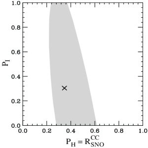
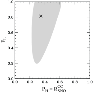
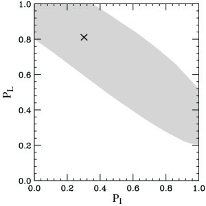
FIG. 1.: Best-fit values and 95.4% C.L. allowed regions for $P_{I}$ versus $P_{H}$, $P_{L}$ versus $P_{H}$, and $P_{L}$ versus $P_{I}$, assuming oscillations to active neutrinos and SSM fluxes ($\beta=1$).

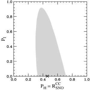
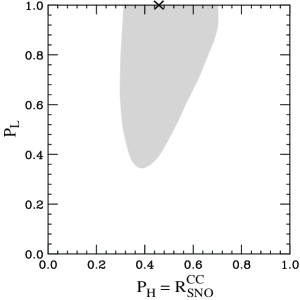
FIG. 2.: Same as Fig. 1 for oscillations to sterile neutrinos.

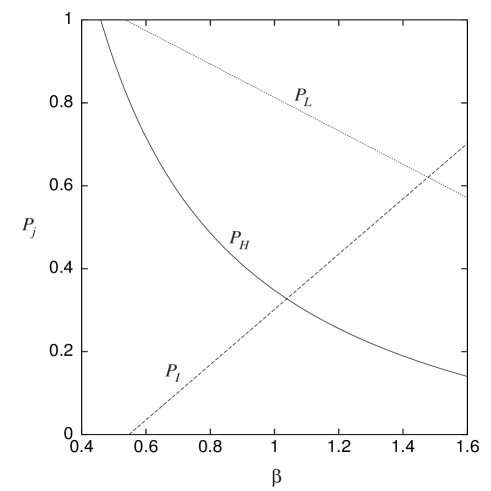
FIG. 3.: Probabilities $P_{H}$, $P_{I}$, and $P_{L}$ for active neutrino oscillations that exactly reproduce the solar neutrino data, plotted versus $\beta$, the ratio of the ⁸B flux normalization to its SSM value.

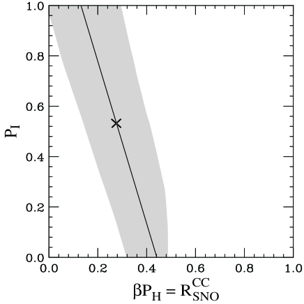
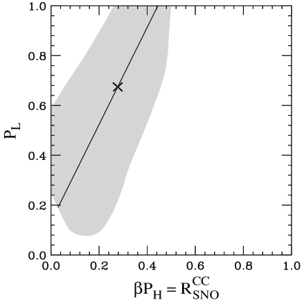
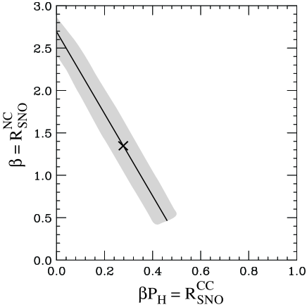
FIG. 4.: The 95.4% C.L. allowed regions from an analysis with free ⁸B flux normalization $\beta$, for $P_{I}$ versus $\beta P_{H}$, $P_{L}$ versus $\beta P_{H}$, $P_{L}$ versus $P_{I}$ and $\beta$ versus $\beta P_{H}$, assuming oscillations to active neutrinos. The line represents solutions with $\chi^{2}=0$. The cross marks the point selected once adiabatic constraints are imposed.

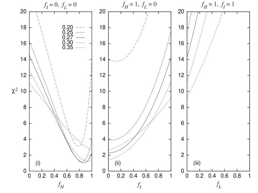
FIG. 5.: $\chi^{2}$ for the LMA solution versus (i) $f_{H}$, with $f_{I}=f_{L}=0$, (ii) $f_{I}$, with $f_{H}=1$ and $f_{L}=0$, and (iii) $f_{L}$, with $f_{H}=f_{I}=1$, where $f_{j}$ is the fraction of $j$-type neutrinos ($j=H,I,$ or $L$) created above resonance, for various values of $\sin^{2}\theta$. SSM fluxes are assumed ($\beta=1$).

FIG. 6.: The 95.4% C. L. and 68.3% C. L. allowed regions from an analysis with $\beta$, $\theta$ and $f_{j}$ free. The best-fit point $(R_{\rm SNO}^{NC},R_{\rm SNO}^{CC})=(1.34,0.28)$, is marked with a cross.

REFERENCES

- [1] B. Cleveland, T. Daily, R. Davis, Jr., J. Distel, K. Lande, C. Lee, P. Wildenhain and J. Ullman, Astropart. Phys. 496, 505 (1998).
- [2] J. Abdurashitov et al., Phys. Rev. C60, 055801 (1999).
- [3] W. Hampel et al., Phys. Lett. B447, 127 (1999).
- [4] M. Altmann et al., Phys. Lett. B490, 16 (2000).
- [5] S. Fukuda et al., hep-ex/0103032.
- [6] J. Bahcall, M. Pinsonneault and S. Basu, astro-ph/0010346.
- [7] S. Fukuda et al., hep-ex/0103033.
- [8] J. Bahcall, P. Krastev and A. Yu. Smirnov, hep-ph/0103179.
- [9] L. Wolfenstein, Phys. Rev. D17, 2369 (1978); V. Barger, K. Whisnant, S. Pakvasa and R. Phillips, Phys. Rev. D22, 2718 (1980); S. Mikheev and A.Yu. Smirnov, Nuovo Cim. C9, 17 (1986).
- [10] KamLAND proposal, Stanford-HEP-98-03.
- [11] V. Barger, D. Marfatia and B. Wood, Phys. Lett. B498, 53 (2001).
- [12] R. Barbieri and A. Strumia, hep-ph/0011307; H. Murayama and A. Pierce, hep-ph/0012075.
- [13] A. McDonald, Nucl. Phys. B (Proc. Suppl) 77, 43 (1999); J. Boger et al. Nucl. Instrum. Meth. A449, 172 (2000).
- [14] V. Barger, D. Marfatia, K. Whisnant and B. Wood, hep-ph/0104095.
- [15] J. Bahcall, P. Krastev and A. Yu. Smirnov, Phys. Rev. D63, 053012 (2000). M. Gonzalez-Garcia, C. Pena-Garay and A. Yu. Smirnov, hep-ph/0012313. J. Bahcall, P. Krastev and A. Yu. Smirnov, Phys. Rev. D62, 093004 (2000); M. Maris and S. Petcov, Phys. Rev. D62, 093006 (2000); J. Bahcall, P. Krastev and A. Yu. Smirnov, Phys. Lett. B477, 401 (2000); M. Gonzalez-Garcia and C. Pena-Garay, hep-ph/0011245; G. Fogli, E. Lisi and D. Montanino, Phys. Lett. B434, 333 (1998); W. Kwong and S. Rosen, Phys. Rev. D54, 2043 (1996).
- [16] V. Barger, R. Phillips, and K. Whisnant, Phys. Rev. D43, 1110 (1991).
- [17] C. Arpesella et al., edited by G. Bellini et al. (University of Milano Press, Milano, 1992) Vols. 1 and 2.
- [18] R. Raghavan, Science 267, 45 (1995); P. Krastev and S. Petcov, Phys. Rev. D53, 1665 (1996).
- [19] S. Parke, Phys. Rev. Lett. 57, 1275 (1986).
- [20] H. Bethe, Phys. Rev. Lett. 56, 1305 (1986); V. Barger, R. Phillips, and K. Whisnant, Phys. Rev. D34, 980 (1986).