QCD analysis of $D$-parameter
in near-to-planar three-jet events

Abstract:

We present the QCD analysis of $D$-parameter distribution in near-to-planar 3-jet $e^{+}e^{-}$ annihilation events. We derive the all-order resummed perturbative prediction and the leading power suppressed non-perturbative corrections both to the mean value and the distribution. Here non-perturbative corrections are larger than in $2$-jet shape observables, so that higher order non-perturbative effects could be relevant. Experimental data (not yet available) are needed in order to cast light on this important point. The technique we develop aims at improving the accuracy of the theoretical description of multi-jet ensembles, in particular in hadron-hadron collisions.

1 Introduction

The analysis of event shape distributions in $e^{+}e^{-}$ has provided various tests of QCD [1] and measurements of the running coupling [2]. The shape observables which have been most intensively studied and tested are: thrust $T$, $C$-parameter, jet mass $M^{2}$ and broadening $B$. Their distributions are collinear and infrared safe (CIS) and therefore can be computed order-by-order in perturbation (PT) theory. Specially interesting is the region of two narrow jets ($1\!-\!T,C,M^{2}/Q^{2},B\ll 1$), where the PT expansion needs to be resummed so that the QCD structure is most intensively probed. The available PT results [3] for these typical $2$-jet observables involve all-order resummation of double- (DL) and single-logarithmic (SL) contributions and matching of the approximate resummed expressions with the exact second order matrix elements.

To make quantitative predictions one needs to go beyond PT calculations and to take into account the $1/Q$–suppressed power corrections arising from the interaction in the confinement region. It has been proposed [4] that these non-perturbative (NP) corrections can be estimated by extrapolating the running coupling into the large distance region. A systematic method for this extrapolation is provided by the dispersive approach [5]. The leading NP corrections to the shape distributions involve a single parameter, usually denoted by $\alpha_{0}$, which is given by the integral of the QCD coupling over the region of small momenta $k\leq\mu_{I}$ (with the infrared scale $\mu_{I}$ conventionally chosen to be $\mu_{I}=2\mathop{\rm Ge\!V}$). They have been computed at two-loop level to take into account effects of non-inclusiveness of jet observables [6]. Such a procedure for computing the $1/Q$–power corrections is consistent with the data and the NP parameter $\alpha_{0}$ has been measured and appears to be universal with a reasonable accuracy [1].

We have recently studied the distribution in the thrust minor $T_{m}$, a CIS shape observable characterising $3$-jet events. It starts at order $\alpha_{\mbox{\scriptsize s}}^{2}$ and measures the radiation out of the event plane in $e^{+}e^{-}$ annihilation. The event plane is defined by the $T$ and $T_{M}$ axes, with $T_{M}$ is the thrust major. The most interesting region in which one probes QCD is that of nearly planar $3$-jet events, $T_{m}\ll T_{M}\sim T$, where PT resummation is needed. The methods developed for the analysis of $2$-jet observables $T,C,M^{2}/Q^{2}$ and $B$ were extended to the case of $T_{m}$ in [7].

In this paper we report the analysis of the distribution in another typical $3$-jet observable, the $D$-parameter which has been introduced in [8]. This is a CIS shape observable which, as $T_{m}$, measures the radiation out of the event plane. In the nearly planar $3$-jet region ($D\ll 1$), the main difference between $D$ and $T_{m}$ is that only soft particles at large angles with respect to the event plane, $p_{\mbox{\scriptsize out}}\sim p_{\mbox{\scriptsize in}}\propto D\ll 1$, contribute to $D$, contrary to the $T_{m}$ case. The fact that energetic hadrons with $p_{\mbox{\scriptsize in}}\gg p_{\mbox{\scriptsize out}}$ do contribute to $T_{m}$, gives rise, in particular, to additional logarithmic enhancement of the NP contribution from the regions where a small transverse momentum energetic gluon is emitted close to the direction of one of the three jets. This difference is similar to that between $B$ and $T,C,M^{2}/Q^{2}$ in $2$-jet events [6]: an energetic hadron emitted near the thrust axis contributes to $B$ but does not contribute to the other shape observables.

Our study is performed with the accuracy necessary to make quantitative predictions. We perform the all-order resummation of DL- and SL-enhanced PT contributions, match it [3] with the exact fixed order matrix element calculation and compute the leading $1/Q$ NP correction at the two-loop order. Actually, the fact that only hadrons at large angles contribute to $D\ll 1$ makes the present analysis significantly simpler than that of $T_{m}$.

We find that, as in the $T_{m}$ case, the structure of the result is quite rich, especially for small $D$ where both the PT and NP components of the $D$ distribution essentially depend on the geometry of the event (the angles between jets). Not only will the analysis of the $D$ distribution provide an alternative measurement of the QCD coupling $\alpha_{\mbox{\scriptsize s}}$. It gives a powerful tool for accessing genuine confinement hadronisation effects, for extracting the NP parameter $\alpha_{0}$ and testing its universality.

The paper is organised as follows. In section 2 we introduce the observable and discuss the characteristic kinematics in the near-to-planar $3$-jet region. In section 3 we discuss the resummation procedure. In section 4 we analyse the PT resummation at SL level. In section 5 we analyse the leading NP corrections in terms of the universal parameter $\alpha_{0}$. In section 6 we report the final result and discuss the necessary ingredients of the one-loop matching. In section 7 we report the numerical analysis of the distribution and the mean. In section 8 we summarise and discuss the results.

2 The observable

The $D$ parameter is defined as [8]

$$D\equiv 27\>\mbox{det}\>\theta\!=\!27\lambda_{1}\lambda_{2}\lambda_{3}\>,\qquad\theta_{\alpha\beta}=\frac{1}{\sum_{h}\left|\>\vec{p}_{h}\>\right|}\sum_{h}\frac{p_{h\alpha}\,p_{h\beta}}{\left|\>\vec{p}_{h}\>\right|}\>,$$ (1)

with $\vec{p}_{h}$ the momentum of the emitted hadron $h$ and $p_{h\alpha}$ its $\alpha$-component ($\alpha=1,2,3$). The eigenvalues $\lambda_{i}$ satisfy the conditions $0\leq\lambda_{i}\leq 1$ and $\sum_{i}\lambda_{i}=1$. We assume the order $\lambda_{3}\leq\lambda_{2}\leq\lambda_{1}$.

To select near-to-planar events we introduce a lower limit $y_{c}$ for the $3$-jet resolution variable $y_{3}$, defined according to the $k_{T}$ (Durham) algorithm [10]. We study the following normalised integrated distribution

$$\begin{split}&\Sigma(D,y_{c})=\frac{1}{\sigma(y_{c})}\sum_{m}\!\int\!{d\sigma_{m}}\>\Theta(y_{3}-y_{c})\>\Theta\left(D\!-\!27\,\mbox{det}\,\theta\right)\>,\\ &\sigma(y_{c})=\sum_{m}\!\int\!{d\sigma_{m}}\>\Theta(y_{3}-y_{c})\>,\end{split}$$ (2)

where $d\sigma_{m}$ denotes the differential distribution in the $m$ final particles with momenta $p_{h}$.

We comment here on the fact that we use the variable $y_{3}$ to select the $3$-jet events (instead of, for instance, the thrust $T$), which makes it easier to interpret the $1/Q$ power corrections that, as we shall see, are present in the D-distribution. Indeed, the difference between the hadron and parton level values of the thrust variable $T$ is known to be of the order of $1/Q$, while the values of $y_{3}$ for hadrons and partons is not affected by $1/Q$ corrections [5]. Therefore, the $1/Q$ contribution to the distribution (2) can be looked upon as a genuine NP correction to the variable $D$. On the contrary, substituting $T<T_{c}$ for $y_{3}>y_{c}$ in the distribution (2), the $1/Q$ correction would have to be shared between $D$ and $T$.

The region of small $D$ and relatively large $y_{c}$ (we consider typical values of $y_{c}$ in the range $0.025-0.1$) corresponds to the region

$$\lambda_{3}\ll\lambda_{2}\mathrel{\mathchoice{\lower 3.6pt\vbox{\halign{$\mathsurround=0pt\displaystyle\hfil#\hfil$\cr<\crcr\sim\crcr}}}{\lower 3.6pt\vbox{\halign{$\mathsurround=0pt\textstyle\hfil#\hfil$\cr<\crcr\sim\crcr}}}{\lower 3.6pt\vbox{\halign{$\mathsurround=0pt\scriptstyle\hfil#\hfil$\cr<\crcr\sim\crcr}}}{\lower 3.6pt\vbox{\halign{$\mathsurround=0pt\scriptscriptstyle\hfil#\hfil$\cr<\crcr\sim\crcr}}}}\lambda_{1}\>,\qquad T_{m}\ll T_{M}\mathrel{\mathchoice{\lower 3.6pt\vbox{\halign{$\mathsurround=0pt\displaystyle\hfil#\hfil$\cr<\crcr\sim\crcr}}}{\lower 3.6pt\vbox{\halign{$\mathsurround=0pt\textstyle\hfil#\hfil$\cr<\crcr\sim\crcr}}}{\lower 3.6pt\vbox{\halign{$\mathsurround=0pt\scriptstyle\hfil#\hfil$\cr<\crcr\sim\crcr}}}{\lower 3.6pt\vbox{\halign{$\mathsurround=0pt\scriptscriptstyle\hfil#\hfil$\cr<\crcr\sim\crcr}}}}T\>.$$ (3)

Here $\lambda_{1},\lambda_{2},y_{3}$ and $T,T_{M}$ are determined by the hard momenta characterising the three jets. The smallest eigenvalue $\lambda_{3}$ and $T_{m}$ are determined by the out-of-event-plane soft momentum component of the particles around and between the jets (inter- and intra-jet radiation). Taking the plane of the event as the $\{y,z\}$-plane, the dominant contribution to $\lambda_{3}$ in the region (3) is given by

$$\lambda_{3}\>\simeq\sum_{h}\frac{p^{2}_{h\,x}}{E_{h}Q}\,.$$ (4)

Due to the energy factor $E_{h}$ in the denominator, $\lambda_{3}$ gets the leading contribution from hadrons with $E_{h}\sim p_{h\,x}$. Instead, the observable $T_{m}$

$$T_{m}=\sum_{h}\frac{|p_{hx}|}{Q}\>,$$ (5)

as mentioned in the Introduction, receives contributions from particles with arbitrary large energies, and in particular those that are quasi-collinear with one of the hard jets.

3 Parton process and resummation

Our first aim is to express the distribution $\Sigma(D,y_{c})$ in terms of parton processes in the near-to-planar region (3). Here the parton events can be treated as $3$-jet events generated by a hard quark-antiquark-gluon system accompanied by an ensemble of secondary partons $k_{i}$. In this region, the quantities $\lambda_{1},\,\lambda_{2},\,T,\,T_{M}$ and the $3$-jet resolution variable $y_{3}$ are determined by the three momenta of the hard quark, antiquark and gluon which we denote by $P_{1},P_{2}$ and $P_{3}$, respectively. Introducing the Born $x$-invariants (for the Born Kinematics see Appendix  A)

$$x_{a}\equiv\frac{2P_{a}Q}{Q^{2}}\>,\qquad 2=x_{1}+x_{2}+x_{3}\>,$$ (6)

we have

$$\begin{split}&\lambda_{1}\,\lambda_{2}=\frac{2(1-x_{1})(1-x_{2})(1-x_{3})}{x_{1}x_{2}x_{3}}\>,\qquad y_{3}=\frac{x_{\min}(1-x_{\max})}{2-x_{\max}-x_{\min}}\>,\end{split}$$ (7)

with

$$x_{\max}=\max\{x_{1},x_{2},x_{3}\}\>,\quad x_{\min}=\min\{x_{1},x_{2},x_{3}\}\>.$$ (8)

At the Born level, all three partons are in the event plane so that $D=\lambda_{3}=0$. With account of secondary partons $k_{i}$, radiation out of the event plane is generated and one gets $\lambda_{3}>0$. At the same time, the hard quark, antiquark and gluon momenta acquire recoils and move out of the event plane. In the near-to-planar region (3), both the hard parton recoil and the secondary parton momenta can be treated as small (soft). To leading order the smallest eigenvalue $\lambda_{3}$ is given by

$$\lambda_{3}\>=\>\sum_{i}\frac{k^{2}_{i\,x}}{\omega_{i}Q}\,,$$ (9)

with $k_{i\,x}$ the out-of-event plane component and $\omega_{i}$ the energy of a secondary soft parton $i$. Corrections are quadratic in the “soft” parameter $k_{x}/Q\sim D\ll 1$. In particular, due to the presence of the energy in the denominator, the contributions from the recoiling hard primary partons $q\bar{q},g$ are of second order (${\cal{O}}\left(D^{2}\right)$) and have been neglected in (9). The quantities $\lambda_{1}\lambda_{2}$ and $y_{3}$ are given, to leading order, by (7) with corrections linear and quadratic in $D$ respectively.

3.1 Resummation of soft radiation

The starting point for the parton resummation of the distribution (2) is the factorisation of soft emission from the hard parton system. The distribution $M^{2}_{n}$ for the emission of $n$ soft partons from the primary $q\bar{q},g$ system can be factorised in the form

$$M^{2}_{n}\,(P_{a},k_{1}\ldots k_{n})\simeq M^{2}_{0}\,(P_{a})\cdot S_{n}\,(P_{a},k_{1}\ldots k_{n})\>,$$ (10)

where we have used the fact that the hard parton recoils can be neglected and the actual $q\bar{q}g$ momenta replaced by their Born values $P_{a}$. The first factor is the squared first order matrix element giving the Born distribution

$$\frac{d\sigma^{(0)}}{dx_{1}dx_{2}}=\frac{C_{F}\alpha_{\mbox{\scriptsize s}}}{2\pi}\>\frac{x_{1}^{2}+x_{2}^{2}}{(1-x_{1})(1-x_{2})}\>,\quad\alpha_{\mbox{\scriptsize s}}=\alpha_{\mbox{\scriptsize s}}(Q)\>,$$ (11)

where, from now on, $x_{1}$ and $x_{2}$ mark the quark and antiquark invariant energy fractions (or vice versa), and $x_{3}=2-x_{1}-x_{2}$ is that of the hard gluon.

The second factor $S_{n}$ describes the distribution for emitting $n$ soft partons $k_{i}$ from the hard $q\bar{q},g$ system. This distribution can also be factorised into the product of independent soft emissions. The structure of this factorisation depends on the required accuracy. Since we aim at SL accuracy, we follow the analysis of [7] in which $S_{n}$ is factorised at two-loop order.

In the region (3), from the factorised expression (10) at parton level we can write

$$\begin{split}&\Sigma(D,y_{c})\simeq\frac{1}{\sigma(y_{c})}\int dx_{1}dx_{2}\,\Theta(y_{3}-y_{c})\left\{C(\alpha_{\mbox{\scriptsize s}})\cdot\frac{d\sigma^{(0)}}{dx_{1}dx_{2}}\cdot S(D,x_{1},x_{2}))\right\},\\ &\sigma(y_{c})\simeq\int dx_{1}dx_{2}\,\Theta(y_{3}-y_{c})\>\frac{d\sigma^{(0)}}{dx_{1}dx_{2}}\>,\end{split}$$ (12)

with $y_{3}$ given by the Born expression (7). The first factor in the curly brackets is the non-logarithmic coefficient $C(\alpha_{\mbox{\scriptsize s}})=1+{\cal{O}}\left(\alpha_{\mbox{\scriptsize s}}\right)$, which is, in general, a function of $y_{3}$ and $D$, and has a finite $D\to 0$ limit. The soft factor $S(D,x_{1},x_{2})$ accumulates all logarithmic dependences on $D$, and is given by

$$\begin{split}S(D,x_{1},x_{2})\>=\>\sum_{n}\frac{1}{n!}\int\prod_{i}^{n}\frac{d^{3}k_{i}}{\pi\omega_{i}}\>S_{n}(P_{a},k_{1}\ldots k_{n})\>\Theta\!\left(\!\lambda_{3}\!-\!\sum_{i}\frac{k^{2}_{ix}}{\omega_{i}Q}\right),\end{split}$$ (13)

(with $\lambda_{3}={D}/{27\lambda_{1}\lambda_{2}}$). Taking the factorised structure of $S_{n}$ at two loops, this expression for $S(D,x_{1},x_{2})$ is accurate to SL level, see [7].

Given the factorised expression for $S_{n}$, in order to sum up the series in (13) in suffices to factorise the theta-function constraint by using the Mellin representation. We obtain

$$S(D,x_{1},x_{2})=\int\frac{d\nu}{2\pi i\nu}\>e^{\nu\lambda_{3}}\>\sigma(\nu,x_{1},x_{2})\>,$$ (14)

where

$$\sigma(\nu,x_{1},x_{2})=\sum_{n}\frac{1}{n!}\int\prod_{i}^{n}\frac{d^{3}k_{i}}{\pi\omega_{i}}\>e^{-\nu\frac{k^{2}_{ix}}{\omega_{i}Q}}\cdot S_{n}(P_{a},k_{1}\ldots k_{n})\>\equiv\>e^{-{\cal{R}}(\nu,x_{1},x_{2})}.$$ (15)

The contour in (14) runs parallel to the imaginary axis with Re $\nu>0$. The near-to-planar region $D\ll 1$ corresponds to the region of large Mellin variable $\nu\gg 1$.

We show that the radiator is given by a PT contribution and a NP correction

$${\cal{R}}(\nu,x_{1},x_{2})={\cal{R}}^{\mbox{\scriptsize PT}}(\nu,x_{1},x_{2})+\delta{\cal{R}}(\nu,x_{1},x_{2})\>.$$ (16)

In the next section we compute the PT contribution at SL level. In section 5 we compute $\delta{\cal{R}}$, the leading $1/Q$ correction including the effect of non-inclusiveness of the $D$-parameter (Milan factor).

4 PT contribution at SL accuracy

To obtain the PT radiator ${\cal{R}}^{\mbox{\scriptsize PT}}(\nu,x_{1},x_{2})$ we follow the procedure described in detail in [7] for the calculation of the $T_{m}$ distribution. The present case is simpler since the hard parton recoil can be neglected. At SL level we have

$$\begin{split}{\cal{R}}^{\mbox{\scriptsize PT}}=\frac{N_{c}}{2}\left(r_{13}+r_{23}-\frac{1}{N_{c}^{2}}\,r_{12}\right),\end{split}$$ (17)

where

$$r_{ab}(\nu,x_{1},x_{2})=\int\frac{d^{3}k}{\pi\omega}w_{ab}(k)\,\left[1-e^{-\nu\frac{k_{x}^{2}}{\omega Q}}\right],\qquad w_{ab}(k)=\frac{\alpha_{\mbox{\scriptsize s}}(k^{2}_{t,ab})}{\pi k^{2}_{t,ab}}\>,$$ (18)

with $w_{ab}(k)$ the soft distribution for the dipole $ab$. Here the running coupling is defined in the physical scheme [11] and $k_{t,\,ab}$ is the invariant transverse momentum of $k$ with respect to the hard parton pair $P_{a},P_{b}$, defined as

$$k^{2}_{t,ab}=\frac{2(P_{a}k)(kP_{b})}{(P_{a}P_{b})}\>.$$ (19)

The unity in the square bracket in (18) takes into account the virtual corrections. The contribution from the source $u(k)=e^{-\nu{k_{x}^{2}}/{\omega Q}}$ results from the exponentiation of real emissions, see (15). To reach SL accuracy one needs to take into account also the correction coming from hard collinear parton splittings, which will be embodied into a redefinition of the hard scales, see later.

4.1 Explicit calculation of the PT radiator

In the laboratory frame the hard parton momenta $P_{a}$ and $P_{b}$ are not back-to-back and the expression of soft dipole distribution $w_{ab}(k)$ is rather cumbersome (see (19)). It is then natural to evaluate $r_{ab}$ starting from its expression in the centre-of-mass frame of the dipole $P_{a}+P_{b}$,

$$P^{*}_{a}\!=\!\frac{Q_{ab}}{2}\>(1,0,0,1)\,,\quad P^{*}_{b}\!=\!\frac{Q_{ab}}{2}\>(1,0,0,-1)\,,\quad Q^{2}_{ab}\!=\!2P_{a}P_{b}\!=\!Q^{2}(x_{a}\!+\!x_{b}-1)\,,$$ (20)

in which the distribution $w_{ab}(k)$ and the phase space are given by

$$w_{ab}(k)=\frac{\alpha_{\mbox{\scriptsize s}}(\kappa^{2})}{\pi\kappa^{2}}\>,\qquad\frac{d^{3}k}{\pi\omega}=d\kappa^{2}\,\frac{d\phi}{2\pi}d\eta\>,$$ (21)

with $\kappa^{2}$, $\eta$ and $\phi$ the squared transverse momentum, the rapidity and the azimuthal angle of the soft gluon, respectively. To compute the dipole radiator $r_{ab}(\nu)$ we need to express the source for our observable $u(k)=e^{-\nu{k^{2}_{x}}/{\omega Q}}$ in the frame (20). While the variable $k_{x}$ is the same in the two frames, $k_{x}=\kappa\sin\phi$, the gluon energy $\omega$ in the laboratory frame (see (63) in Appendix A) is given, in terms of the dipole c.m.s. variables

$$\omega=\kappa\left(A_{ab}\cosh(\eta\!+\!\eta^{0}_{ab})-\sqrt{A_{ab}^{2}\!-\!1}\>\cos\phi\right)\>,$$ (22)

with $A_{ab}$ and $\eta^{0}_{ab}$ the following functions of $x_{a},x_{b}$

$$\begin{split}&A_{ab}=\frac{Q}{Q_{ab}}\sqrt{x_{a}x_{b}}=\sqrt{\frac{x_{a}x_{b}}{x_{a}+x_{b}-1}}\>,\qquad\tanh\eta^{0}_{ab}=\frac{x_{a}\!-\!x_{b}}{x_{a}\!+\!x_{b}}\>.\end{split}$$ (23)

Finally, using the frame (20), the $r_{ab}$ radiator can be written in the form

$$r_{ab}(\nu,x_{1},x_{2})=\int_{0}^{Q^{2}}\frac{d\kappa^{2}}{\kappa^{2}}\frac{\alpha_{\mbox{\scriptsize s}}(\kappa^{2})}{\pi}\int_{-\pi}^{\pi}\frac{d\phi}{2\pi}\int_{-\eta_{M}}^{\eta_{M}}d\eta\left(1\!-\!e^{-\nu\frac{\kappa}{Q}\,\tau}\right),\quad\eta_{M}=\ln\frac{Q_{ab}}{\kappa}\>,$$ (24)

where $\tau$ is the following function of $\eta$ and $\phi$

$$\tau=\frac{\sin^{2}\phi}{A_{ab}\cosh(\eta\!+\!\eta^{0}_{ab})-\sqrt{A_{ab}^{2}\!-\!1}\,\cos\phi}\>.$$ (25)

Note that, since $Q_{ab}\sim Q$, to SL accuracy, we do not care for the precise upper limit in $\kappa$ as long as it is of order $Q$.

The calculation of $r_{ab}$ is performed in Appendix B and one finds, to SL accuracy,

$$r_{ab}(\nu,x_{1},x_{2})=2\int_{{Q^{2}}/{\nu}}^{Q^{2}}\frac{d\kappa^{2}}{\kappa^{2}}\frac{\alpha_{\mbox{\scriptsize s}}(\kappa^{2})}{\pi}\ln\frac{Q_{ab}}{\kappa}+2\int_{{Q^{2}}/{\nu^{2}}}^{{Q^{2}}/{\nu}}\frac{d\kappa^{2}}{\kappa^{2}}\frac{\alpha_{\mbox{\scriptsize s}}(\kappa^{2})}{\pi}\ln\left(\frac{e^{\gamma_{E}}\,\nu\,\kappa}{2A_{ab}Q}\right).$$ (26)

Combining together the various pieces and recalling the definition of $A_{ab}$ in (23) we find the full PT radiator

$${\cal{R}}^{\mbox{\scriptsize PT}}(\nu,x_{1},x_{2})\>=\>C_{F}\left[\,r_{1}(\nu,Q_{1})+r_{2}(\nu,Q_{2})\,\right]\>+\>C_{A}\,r_{3}(\nu,Q_{3})\>,$$ (27)

where the contribution of the hard parton $\#a$ is given by

$$r_{a}(\nu,Q_{a})=2\int_{{Q^{2}}/{\nu}}^{Q^{2}}\frac{d\kappa^{2}}{\kappa^{2}}\frac{\alpha_{\mbox{\scriptsize s}}(\kappa^{2})}{2\pi}\,\ln\frac{\xi_{a}Q_{a}}{\kappa}\>+\>2\int_{{Q^{2}}/{\nu^{2}}}^{{Q^{2}}/{\nu}}\frac{d\kappa^{2}}{\kappa^{2}}\frac{\alpha_{\mbox{\scriptsize s}}(\kappa^{2})}{2\pi}\ln\left(\frac{e^{\gamma_{E}}\,\nu\,\kappa\,Q_{a}}{2x_{a}Q^{2}}\right)\>.$$ (28)

Here the hard scales $Q_{a}$ are

$$\begin{split}&Q^{2}_{1}=Q^{2}_{2}=2(P_{1}P_{2})=Q^{2}(1-x_{3})\>,\qquad\\ &Q^{2}_{3}=\frac{2(P_{1}P_{3})(P_{3}P_{2})}{(P_{1}P_{2})}=Q^{2}\frac{(1-x_{1})(1-x_{2})}{(1-x_{3})}\>.\end{split}$$ (29)

In (28) we have included into the first term the rescaling factor $\xi_{a}$

$$\xi_{1}=\xi_{2}=e^{-3/4}\>,\qquad\xi_{3}=e^{-\beta_{0}/4N_{c}}\>,$$ (30)

to take into account the hard collinear splittings of the quark and the gluon. These constants, as well as the precise expressions for the geometry dependent scales $Q_{a}$, are important in order to incorporate in the final result (27) for the radiator all terms of the order of $\alpha_{\mbox{\scriptsize s}}^{n}\ln^{n+1}\nu$ and $\alpha_{\mbox{\scriptsize s}}^{n}\ln^{n}\nu$.

To first order we find

$$r_{a}(\nu,Q_{a})=\frac{\alpha_{\mbox{\scriptsize s}}}{2\pi}\>\ln^{2}\left(\frac{e^{\gamma_{E}}\,\nu\,\xi_{a}\,Q_{a}^{2}}{2x_{a}Q^{2}}\right)+\ldots$$ (31)

This result corresponds, at DL level, to a half of the DL radiator in the $T_{m}$ case [7]. The relative factor $1/2$ is due to the fact that in the $T_{m}$ case the contribution to the observable is linear in the angle with respect to the event plane, while it is quadratic in the $D$ case.

The first order contribution to the PT part of the distribution (12) is obtained by performing the Mellin integral in (14). We find

$$\frac{d\Sigma^{\mbox{\scriptsize PT}}(D,y_{c})}{d\ln D}=\frac{\alpha_{\mbox{\scriptsize s}}}{2\pi}\left\{2C_{T}\,\ln\frac{1}{D}+\bar{G}_{11}(y_{c})\right\}+\>{\cal{O}}\left(\alpha_{\mbox{\scriptsize s}}^{2}\right),$$ (32)

with $C_{T}=2C_{F}+C_{A}$ the sum of the colour factors — the total colour charge of the hard $q\bar{q},g$ system. Here $\bar{G}_{11}$ is given by

$$\bar{G}_{11}(y_{c})=\int dx_{1}dx_{2}\Theta(y_{3}-y_{c})\frac{d\sigma^{(0)}}{\sigma(y_{c})dx_{1}dx_{2}}\,G_{11}(x_{1},x_{2})\>,$$ (33)

with

$$G_{11}(x_{1},x_{2})=2C_{T}\,\ln 27\lambda_{1}\lambda_{2}\>+\>2C_{F}\left[\ln\frac{\xi_{1}\,Q_{1}^{2}}{2x_{1}Q^{2}}+\ln\frac{\xi_{2}\,Q_{2}^{2}}{2x_{2}Q^{2}}\right]+2C_{A}\,\ln\frac{\xi_{3}\,Q_{3}^{2}}{2x_{3}Q^{2}}\>.$$ (34)

We have checked that this function correctly describes the first non-logarithmic correction by comparing with the result of the numerical program EVENT2 [12] for $y_{c}=0.025,\,0.05$ and $0.1$.

5 NP calculation

We follow the usual procedure [6] for computing the leading NP corrections, including two-loop order to take into account the non-inclusiveness of jet observables. We start from the PT expression (24) and then:

• we represent the coupling by the dispersive integral [5]

  $$\frac{\alpha_{\mbox{\scriptsize s}}(\kappa^{2})}{\kappa^{2}}=\int_{0}^{\infty}\frac{dm^{2}\,\alpha_{\mbox{\scriptsize eff}}(m^{2})}{(\kappa^{2}+m^{2})^{2}}\>;$$ (35)

• we substitute $\sqrt{\kappa^{2}+m^{2}}$ for the momentum $\kappa$ in the source in (24);

• we take the leading part of the integrand for small $\kappa$ and $m$ by linearising the source

  $$\left[1-e^{-\nu\frac{\sqrt{\kappa^{2}+m^{2}}}{Q}\tau}\right]\>\to\>\nu\frac{\sqrt{\kappa^{2}+m^{2}}}{Q}\tau\>,$$ (36)

  since the NP part of the “effective coupling” $\delta\alpha_{\mbox{\scriptsize eff}}(m)$ has a support only at small $m$;

• we multiply this expression by the Milan factor ${\cal{M}}$, computed at two-loop order, to take into account effects of non-inclusiveness of jet observables.

For the $\{ab\}$-dipole contribution this procedure gives

$$\begin{split}\delta r_{ab}(\nu,x_{1},x_{2})=\nu{\cal{M}}\!\int\!dm^{2}\frac{\delta\alpha_{\mbox{\scriptsize eff}}(m)}{\pi}\frac{-d}{dm^{2}}\!\int\frac{d^{2}\kappa}{\pi(\kappa^{2}+m^{2})}\frac{\sqrt{\kappa^{2}+m^{2}}}{Q}\int_{-\infty}^{\infty}d\eta\,\tau(\eta)\>,\end{split}$$ (37)

where $\tau$ is the function of $x_{1},x_{2}$ defined in (25). It is related with the ratio of transverse momentum to energy and therefore decreases exponentially in rapidity. This allows us to extend to infinity the $\eta$ integrals by setting $\eta_{M}=\infty$.

Here lies the main difference with the $T_{m}$ case in which the observable was uniform in rapidity so that the corresponding NP radiator involved a divergent rapidity integral. There one had to keep the hard parton recoil momentum which provided an effective cutoff to the rapidity integral and resulted in a $\log$–enhanced NP contribution.

We find the leading NP correction to the $\{ab\}$-radiator

$$\delta r_{ab}(\nu,x_{1},x_{2})=\nu\,\frac{a^{\mbox{\scriptsize NP}}}{Q}g_{ab}(x_{1},x_{2})\>,$$ (38)

where $g_{ab}$ is the geometry dependent function

$$g_{ab}(x_{1},x_{2})\equiv\int_{-\pi}^{\pi}\frac{d\phi}{2\pi}\int_{-\infty}^{\infty}\frac{d\eta\>\sin^{2}\phi}{A_{ab}\cosh\eta-\cos\phi\sqrt{A_{ab}^{2}-1}}\>,$$ (39)

and $a^{\mbox{\scriptsize NP}}$ is the NP parameter

$$a^{\mbox{\scriptsize NP}}=2{\cal{M}}\int dm\frac{\delta\alpha_{\mbox{\scriptsize eff}}(m)}{\pi}\>.$$ (40)

Combining all pieces we obtain the $1/Q$ correction to the radiator

$$\delta{\cal{R}}(\nu)=\nu\,\frac{a^{\mbox{\scriptsize NP}}}{Q}\Delta(x_{1},x_{2})\>,\qquad\Delta=\frac{N_{c}}{2}\left(g_{13}+g_{23}-\frac{1}{N_{c}^{2}}\,g_{12}\right)\>.$$ (41)

After merging the PT and NP corrections we can write the NP parameter in the form

$$a^{\mbox{\scriptsize NP}}=\frac{4\mu_{I}}{\pi^{2}}{\cal{M}}\left\{\alpha_{0}(\mu_{I})-\bar{\alpha}_{s}-\beta_{0}\,\frac{\bar{\alpha}_{s}^{2}}{2\pi}\left(\ln\frac{Q}{\mu_{I}}+\frac{K}{\beta_{0}}+1\right)\right\}\>,\qquad\bar{\alpha}_{s}=\alpha_{\overline{\mbox{\scriptsize MS}}}(Q)\>,$$ (42)

where

$$\alpha_{0}(\mu_{I})\equiv\frac{1}{\mu_{I}}\int_{0}^{\mu_{I}}\!dk\,\,\alpha_{\mbox{\scriptsize s}}(k^{2})\,.$$

The term proportional to $K$ accounts for the mismatch between the $\overline{\mbox{\scriptsize MS}}$ and the physical scheme [11] and reads

$$K=N_{c}\left(\frac{67}{18}-\frac{\pi^{2}}{6}\right)-\frac{5n_{f}}{9}\>.$$ (43)

For the analytical expression of the Milan factor ${\cal{M}}$ see [13]. To quantify the parameter $a^{\mbox{\scriptsize NP}}$ we recall the expression for the NP shift $\Delta_{T}$ in the thrust distribution [6],

$$\Delta_{T}=2C_{F}\frac{a^{\mbox{\scriptsize NP}}}{Q}\>.$$ (44)

6 Final result

We are now in a position to obtain the full distribution $\Sigma(D,y_{c})$ in (12) to the standard accuracy. First we obtain the PT expression for the soft factor $S^{\mbox{\scriptsize PT}}(D,x_{1},x_{2})$ by performing the Mellin integral (14) with the PT radiator (27). Then, using the exact result of the ${\cal{O}}\left(\alpha_{\mbox{\scriptsize s}}^{2}\right)$ matrix element calculation, we compute the first correction of the coefficient function $C(\alpha_{\mbox{\scriptsize s}})$ in (12). This allows us to perform the matching of the resummed and the exact result to this order. Finally, we include the leading NP correction from (41).

6.1 PT resummed distribution

The PT contribution is given by

$$\begin{split}&S^{\mbox{\scriptsize PT}}(D,x_{1},x_{2})=\int\frac{d\nu\,e^{\,\nu\lambda_{3}}}{2\pi i\nu}\>e^{-{\cal{R}}^{\mbox{\scriptsize PT}}(\nu,x_{1},x_{2})}\simeq\frac{e^{-{\cal{R}}^{\mbox{\scriptsize PT}}\left(\lambda_{3}^{-1}\!,x_{1},x_{2}\right)}}{\Gamma(1+{\cal{R}}^{\prime})}\>,\\ &{\cal{R}}^{\prime}\equiv-D\partial_{D}\,{\cal{R}}^{\mbox{\scriptsize PT}}\left(D^{-1}\!,x_{1},x_{2}\right),\end{split}$$ (45)

This evaluation of the Mellin integral is accurate to SL level, (see e.g. [7]). In the calculation of the logarithmic derivative of ${\cal{R}}$ the precise expression for the hard scale $Q_{a}$ in $r_{a}(\nu,Q_{a})$ is beyond SL accuracy as long as it is of order $Q$. We can use then $Q$ as a common hard scale in the SL functions $r^{\prime}$, and substitute the logarithmic derivative of the radiator ${\cal{R}}^{\prime}$ with

$${\cal{R}}^{\prime}_{T}\equiv C_{T}\,\int_{(DQ)^{2}}^{DQ^{2}}\frac{d\kappa^{2}}{\kappa^{2}}\frac{\alpha_{\mbox{\scriptsize s}}(\kappa^{2})}{\pi}\>,$$ (46)

where we have explicitly used the expression (26).

Again, to SL accuracy, we can expand the radiator in the exponent of (45) and write

$${\cal{R}}^{\mbox{\scriptsize PT}}\left(\lambda_{3}^{-1}\!,x_{1},x_{2}\right)={\cal{R}}^{\mbox{\scriptsize PT}}\left(D^{-1}\!,x_{1},x_{2}\right)+{\cal{R}}^{\prime}_{T}\cdot\ln(27\lambda_{1}\lambda_{2})\>,$$ (47)

where ${\cal{O}}\left(\alpha_{\mbox{\scriptsize s}}\right)$ corrections have been neglected. We conclude by giving the SL–accurate expression

$$\begin{split}S^{\mbox{\scriptsize PT}}(D,x_{1},x_{2})=e^{-{\cal{R}}^{\mbox{\scriptsize PT}}\left(D^{-1},x_{1},x_{2}\right)}\cdot\frac{e^{-{\cal{R}}^{\prime}_{T}\,\ln(27\lambda_{1}\lambda_{2})}}{\Gamma(1+{\cal{R}}^{\prime}_{T})}\>.\end{split}$$ (48)

Using the expression of the PT radiator given in Appendix B and ${\cal{R}}^{\prime}_{T}$ given in (46), this distribution can be written as

$$\ln S^{\mbox{\scriptsize PT}}(D,x_{1},x_{2})=L\,g_{1}(\bar{\alpha}\,L)+g_{2}(\bar{\alpha}\,L,x_{1},x_{2})\>,\quad\bar{\alpha}=\alpha_{\overline{\mbox{\scriptsize MS}}}(Q)\>,\quad L=-\ln D\>,$$ (49)

where only the logarithmic terms in $D$ were kept, while the finite corrections ${\cal{O}}\left(\alpha_{\mbox{\scriptsize s}}\right)$ dropped. This precaution is necessary in order to properly set up the procedure for matching the resummed expression with the exact fixed order result. The DL contribution, the first term in (49), does not depend on $x_{1},x_{2}$. Therefore the dependence on the event geometry emerges at the level of subleading SL effects. In the first order we recover from (49) the result already obtained in (32).

Finally, the resummed PT distribution is given by

$$\Sigma^{\mbox{\scriptsize PT}}(D,y_{c})=\int dx_{1}dx_{2}\Theta(y_{3}-y_{c})\frac{d\sigma^{(0)}}{\sigma(y_{c})dx_{1}dx_{2}}\>S^{\mbox{\scriptsize PT}}(D,x_{1},x_{2})\>.$$ (50)

6.2 Matching resummed and fixed-order prediction

Here we consider the matching with the exact result of order $\alpha_{\mbox{\scriptsize s}}^{2}$, which allows us to compute the first order contribution to the coefficient function $C(\alpha_{\mbox{\scriptsize s}})$ in (12). The exact first order result reads

$$\Sigma_{\mbox{\scriptsize exact}}^{\mbox{\scriptsize PT}}(D,y_{c})=1+\frac{\alpha_{\mbox{\scriptsize s}}}{2\pi}\left(-C_{T}\ln^{2}\frac{1}{D}-\bar{G}_{11}(y_{c})\,\ln\frac{1}{D}+c_{1}(D,y_{c})\right)+{\cal{O}}\left(\alpha_{\mbox{\scriptsize s}}^{2}\right)\>,$$ (51)

where $\bar{G}_{11}(y_{c})$ is defined in (33) and $c_{1}(D,y_{c})$ is a function (regular at $D=0$) which we calculate numerically by using the four–parton numerical program EVENT2 [12]. This gives

$$C(\alpha_{\mbox{\scriptsize s}})=1+\frac{\alpha_{\mbox{\scriptsize s}}}{2\pi}c_{1}(D,y_{c})+\ldots$$ (52)

In fig. 1 we report $c_{1}(D,y_{c})$ as a function of $D$ for three values of $y_{c}$.

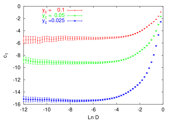
Figure 1: The first order coefficient function for three different values of $y_{c}$.

We define the three matched expressions:

• Log-R matching:

  $$\Sigma^{\mbox{\scriptsize PT}}_{\mbox{\scriptsize mat}}(D,y_{c})\equiv e^{\frac{\alpha_{\mbox{\scriptsize s}}}{2\pi}\,c_{1}(D,y_{c})}\cdot\Sigma^{\mbox{\scriptsize PT}}(D,y_{c})\>,$$ (53)

• R-matching:

  $$\begin{split}\Sigma^{\mbox{\scriptsize PT}}_{\mbox{\scriptsize mat}}(D,y_{c})\equiv\left(1+\frac{\alpha_{\mbox{\scriptsize s}}}{2\pi}c_{1}(0,y_{c})\right)\cdot\Sigma^{\mbox{\scriptsize PT}}(D,y_{c})\>+\frac{\alpha_{\mbox{\scriptsize s}}}{2\pi}\,\left(c_{1}(D,y_{c})-c_{1}(0,y_{c})\right)\>,\end{split}$$ (54)

• modified R-matching:

  $$\Sigma^{\mbox{\scriptsize PT}}_{\mbox{\scriptsize mat}}(D,y_{c})\equiv\left(1+\frac{\alpha_{\mbox{\scriptsize s}}}{2\pi}\,c_{1}(D,y_{c})\right)\cdot\Sigma^{\mbox{\scriptsize PT}}(D,y_{c})\>.$$ (55)

It is easy to see that each of these expressions reproduces the first order result (51) and accounts for all terms of order $\alpha_{\mbox{\scriptsize s}}^{n}\,\ln^{m}D$ with $m\geq 2n\!-\!2$. To obtain also the $\alpha_{\mbox{\scriptsize s}}^{n}\,\ln^{2n-3}D$ terms one needs a second order matching (${\cal{O}}\left(\alpha_{\mbox{\scriptsize s}}^{3}\right)$ exact matrix element calculation) which requires five-parton generators [14], [15]. The matching procedure becomes more involved and will be discussed in [16].

6.3 Including NP corrections

We now consider the distribution with the NP corrections included. Using the expression (41) for the NP radiator, we have

$$\begin{split}S(D,x_{1},x_{2})=\int\frac{d\nu\,e^{\,\nu\lambda_{3}}}{2\pi i\nu}\>e^{-\left\{\nu\,\frac{a^{\mbox{\scriptsize NP}}}{Q}\,\Delta+{\cal{R}}^{\mbox{\scriptsize PT}}(\nu)\right\}}=S^{\mbox{\scriptsize PT}}\left(D\!-\!\delta D,\,x_{1},x_{2}\right)\>,\end{split}$$ (56)

where

$$\delta D=\frac{a^{\mbox{\scriptsize NP}}}{Q}\cdot{\cal{D}}(x_{1},x_{2})\>,\quad{\cal{D}}(x_{1},x_{2})=27\lambda_{1}\lambda_{2}\,\Delta(x_{1},x_{2})\>.$$ (57)

As for other shape observables, we have embodied the leading NP correction as a $1/Q$ shift of the argument of the PT distribution. The magnitude of the shift is determined by the product of the universal NP parameter and the geometry dependent function ${\cal{D}}(x_{1},x_{2})$ with $\Delta(x_{1},x_{2})$ given in (41).

The final expression that includes the NP correction is given (for instance, in the Log-R matching scheme) by

$$\Sigma(D,y_{c})=\int dx_{1}dx_{2}\Theta(y_{3}-y_{c})\frac{d\sigma^{(0)}}{\sigma(y_{c})dx_{1}dx_{2}}\,e^{\frac{\alpha_{\mbox{\scriptsize s}}}{2\pi}\,c_{1}(D^{\prime},y_{c})}\cdot S^{\mbox{\scriptsize PT}}(D^{\prime},x_{1},x_{2})\>,$$ (58)

where $D^{\prime}$ is the shifted variable

$$\frac{1}{D^{\prime}}=\frac{1}{D-\delta D}-\frac{1}{1-\delta D}+1\>.$$ (59)

The two last terms in (59) are relevant only at large $D$ and have been added as to ensure the correct normalisation of the distribution, $D^{\prime}=1$ at $D=1$.

6.4 Mean value

We can also consider the mean value of $D$ at fixed $y_{c}$ defined as

$$\left\langle D\right\rangle=\int_{0}^{1}dDD\>\frac{d\Sigma(D,y_{c})}{dD}\>.$$ (60)

The integral is dominated by the region of finite $D$ where the secondary partons are all hard, and out of the event plane, so that no logarithmic enhancements are involved here. The PT contribution $\left\langle D\right\rangle^{\mbox{\scriptsize PT}}$ should be then obtained from a fixed order calculation. We have to add to it, however, a NP correction

$$\left\langle D\right\rangle=\left\langle D\right\rangle^{\mbox{\scriptsize PT}}+\left\langle D\right\rangle^{\mbox{\scriptsize NP}}\>.$$ (61)

The NP correction is determined by soft (small transverse momentum) partons and can be obtained from the present analysis, cf. [7]. It is simply related with the average value of the shift as follows

$$\left\langle D\right\rangle^{\mbox{\scriptsize NP}}=\frac{a^{\mbox{\scriptsize NP}}}{Q}\,\int dx_{1}dx_{2}\Theta(y_{3}-y_{c})\frac{d\sigma^{(0)}}{\sigma(y_{c})dx_{1}dx_{2}}\cdot{\cal{D}}(x_{1},x_{2})\>,$$ (62)

with ${\cal{D}}(x_{1},x_{2})$ given in (57).

7 Numerical analysis

We report here the numerical results for some typical values of $y_{c}$. Data are not yet available. The results depend on the two parameters $\alpha_{\overline{\mbox{\scriptsize MS}}}(M_{Z})$ and $\alpha_{0}(\mu_{I})$ (with $\mu_{I}=2\mathop{\rm Ge\!V}$) which values we fix in the range determined by the $2$-jet shape analysis, see for instance  [17].

In fig. 2 we plot, as a function of $Q$, the mean value $\left\langle D\right\rangle$ given in (60) for $y_{c}=0.05$. The leading order PT contribution is obtained from EVENT2 [12]. The next-to-leading order PT contribution is obtained from DEBRECEN [14]. The NP contribution is given by (62).

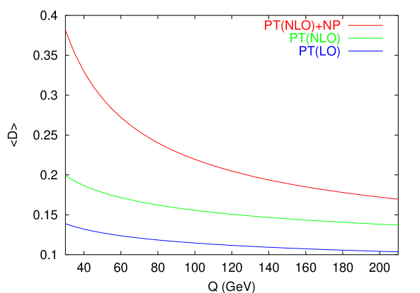
Figure 2: The mean value $\left\langle D\right\rangle$ as a function of $Q$ for $y_{c}=0.05$. Here we have taken $\alpha_{\overline{\mbox{\scriptsize MS}}}(M_{Z})=0.118$ and the NP parameter $\alpha_{0}(2\mathop{\rm Ge\!V})=0.44$.

We see that the NP correction is large up to LEP-II energies. Actually, the coefficient $\Delta(x_{1},x_{2})$ of the NP correction is large due to the fact that one of the three radiating hard partons is the gluon whose contribution to the NP radiation is proportional to its large colour charge, see (41).

In fig. 3 we plot the mean value $\left\langle D\right\rangle$ given in (60) for three different values of $y_{c}$ at $Q=91.2\mathop{\rm Ge\!V}$. The mean value decreases with $y_{c}$ decreasing. This is expected since decreasing $y_{c}$ one includes configurations in which the hard gluon become close to one of the quarks, so that the independent radiation off the gluon gets suppressed.

Figure 3: The mean value $\left\langle D\right\rangle$ as a function of $y_{c}$ for $Q=91.2\mathop{\rm Ge\!V}$ for $\alpha_{\overline{\mbox{\scriptsize MS}}}(M_{Z})$ and $\alpha_{0}(\mu_{I})$ taken at the values of the previous figure.

In figs. 4, 5 and 6 we plot the distributions $\Sigma(D,y_{c})$ for three values of $y_{c}$ for $Q=91.2\mathop{\rm Ge\!V}$. The PT distribution is given by the first order Log-R matched expression in (53). (The second order matching will be presented elsewhere [16].) The full distribution is given by the expression (58). The PT peak is shifted to the right by an amount of order of the NP part of the mean values, see fig. 3. The shift of the PT distribution is not uniform since the $x_{1},x_{2}$–dependent shift has been averaged over the Born distribution.

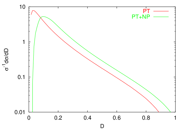
Figure 4: The distribution for $Q=91.2\mathop{\rm Ge\!V}$ and $y_{c}=0.025$ for $\alpha_{\overline{\mbox{\scriptsize MS}}}(M_{Z})=0.118$ and the NP parameter $\alpha_{0}(\mu_{I})=0.52$ at $\mu_{I}=2\mathop{\rm Ge\!V}$.

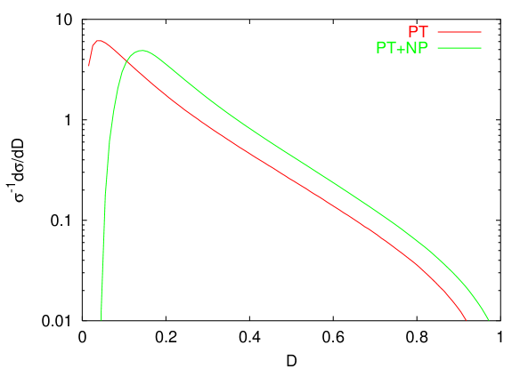
Figure 5: The distribution for $Q=91.2\mathop{\rm Ge\!V}$ and $y_{c}=0.5$ for $\alpha_{\overline{\mbox{\scriptsize MS}}}(M_{Z})=0.118$ and the NP parameter $\alpha_{0}(\mu_{I})=0.52$ at $\mu_{I}=2\mathop{\rm Ge\!V}$.

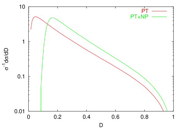
Figure 6: The distribution for $Q=91.2\mathop{\rm Ge\!V}$ and $y_{c}=0.1$ for $\alpha_{\overline{\mbox{\scriptsize MS}}}(M_{Z})=0.118$ and the NP parameter $\alpha_{0}(\mu_{I})=0.52$ at $\mu_{I}=2\mathop{\rm Ge\!V}$.

8 Discussion and conclusion

The aim of the present study is the understanding of the structure of multi-jet events in $e^{+}e^{-}$. To master this field is important, especially, for hadron-hadron collisions where the QCD events involve more than two jets.

This is the second near-to-planar three-jet shape variable, after $T_{m}$, studied at an accuracy sufficient to make quantitative predictions (SL resummation, matching with fixed order, NP corrections). The main difference between the $D$-parameter and $T_{m}$ is the dependence of the observable on particle rapidity. Actually, $T_{m}$ is uniform in rapidity, while $D$ is exponentially dumped. This feature has important consequences both at PT and NP level.

On the PT side, the hard parton recoil explicitly enters the observable in the $T_{m}$ case. On the contrary, in the $D$ case it gives rise to corrections beyond SL accuracy. This in turn implies that the PT $D$ distribution depends only on the geometry of the event (the angles between jets) and not on its colour configuration.

In what concerns NP corrections, one finds that in the $D$ case only soft radiation at large angles contributes to the NP shift. As a consequence, the shift is not logarithmically enhanced, as was the case of $T_{m}$. This is the same difference that occurs between $1-T,C,M^{2}/Q^{2}$ and $B$ jet shapes in the two-jet case.

We observe that the shift for the $D$ parameter is larger than is typical for 2-jet observables. This is explained by the fact that in 3-jet events we have three hard radiating partons whose total colour charge $2C_{F}+C_{A}$ is significantly larger than $2C_{F}$, the total colour charge of a two-jet system. As a consequence, while for 2-jet observables higher order NP effects come into play below the peak of the distribution, for the $D$ parameter they are already relevant in the proximity of the peak. This calls for a deeper analysis that would address higher powers in $1/Q$, for example, along the lines of Korchemsky-Sterman approach which was recently developed for some 2-jet observables in [18]. The comparison with experimental data (not yet available) would shed light on this important point.

Near-to-planar 3-jet events provide a new method to measure the fundamental QCD parameter $\alpha_{\mbox{\scriptsize s}}(M_{Z})$ and to have a further test of the universality of genuine NP effects in jet physics.

Appendix A Born kinematics

We select the event plane in such a way that the two Born momenta with the maximum and minimum $x$-component are given by

$$\begin{split}&P_{\max}=E(x_{\max},0,0,x_{\max})\>,\qquad P_{\min}=E(x_{\min},0,-T_{M},-t_{\min})\>.\end{split}$$ (63)

with $Q=2E$ and

$$\begin{split}x_{\max}\!=\!T\>,\quad x_{\min}\!=\!1\!-\!\frac{T}{2}(1\!+\!\rho)\>,\quad t_{\min}\!=\!\frac{T}{2}\!-\!\rho\left(1-\frac{T}{2}\right)\>,\quad\rho\equiv\sqrt{1\!-\!\frac{T_{M}^{2}}{1\!-\!T}}\>,\end{split}$$ (64)

so that the thrust major is

$$T_{M}=\frac{2}{x_{\max}}\sqrt{(1-x_{1})(1-x_{2})(1-x_{3})}\>.$$ (65)

To define these massless momenta one needs that $T$ and $T_{M}$ are restricted to the region

$$\frac{2(1-T)\sqrt{2T-1}}{T}<T_{M}<\sqrt{1-T}\>.$$ (66)

In this paper we consider $T,T_{M}$ restricted to this region.

Appendix B The PT radiator

Here we compute the radiator component $r_{ab}(\nu)$ given in (24). We change integration variable from $\eta$ to $\tau$ with the Jacobian

$$d\eta=-\frac{d\tau}{\tau}\,K(\tau)\>,\qquad K(\tau)=\frac{\sin^{2}\phi}{\sqrt{\left(\sin^{2}\phi+\tau\sqrt{A^{2}\!-\!1}\,\cos\phi\right)^{2}-\tau^{2}A^{2}}}\>.$$ (67)

In this appendix we set $A_{ab}\to A$ and $\eta^{0}_{ab}\to\eta_{0}$ defined in (23). The $\eta$-integral can be divided into the positive and negative rapidity regions and one has

$$r_{ab}(\nu)=r_{ab}^{+}(\nu)+r_{ab}^{-}(\nu)\>,$$ (68)

where

$$r_{ab}^{\pm}(\nu)=2\int_{0}^{Q}\frac{d\kappa}{\kappa}\frac{\alpha_{\mbox{\scriptsize s}}(\kappa^{2})}{\pi}\int_{-\pi}^{\pi}\frac{d\phi}{2\pi}\int_{\tau_{M}^{\pm}}^{\tau_{0}}\frac{d\tau}{\tau}\,K(\tau)\left(1-e^{-\nu\frac{\kappa}{Q}\tau}\right).$$ (69)

The limits are for $\eta=\pm\eta_{0}$ and $\eta=\eta_{M}$

$$\tau_{0}=\frac{\sin^{2}\phi}{A\!-\!\sqrt{A^{2}\!-\!1}\,\cos\phi}\>,\qquad\tau_{M}^{\pm}=\frac{\sin^{2}\phi}{A\cosh(\eta_{M}\pm\eta_{0})\!-\!\sqrt{A^{2}\!-\!1}\,\cos\phi}\>.$$ (70)

The limit $\tau_{M}^{\pm}$ is a function of $\kappa$ given, for small $\kappa$, by

$$\tau_{M}^{\pm}(\kappa)\simeq\frac{2\sin^{2}\phi}{A}\frac{\kappa}{Q^{\pm}_{ab}}\>,\qquad Q_{ab}^{\pm}=Q_{ab}e^{\pm\eta_{0}}\>.$$ (71)

In (69) we can substitute, to SL accuracy, the factor $[1-e^{-\nu\frac{\kappa}{Q}\,\tau}]$ by the effective cutoff (89) and we obtain

$$r_{ab}^{\pm}(\nu)\simeq 2\int_{0}^{Q}\frac{d\kappa}{\kappa}\frac{\alpha_{\mbox{\scriptsize s}}(\kappa^{2})}{\pi}\int_{-\pi}^{\pi}\frac{d\phi}{2\pi}\int_{\tau_{M}^{\pm}}^{\tau_{0}}\frac{d\tau}{\tau}\,K(\tau)\>\vartheta\left(\tau-\frac{Q}{\bar{\nu}\kappa}\right).$$ (72)

In order to reach SL accuracy, we have to take the running coupling at two loops and include the non-soft part of the parton splitting function. Before discussing this case, it is instructive to consider the first order term in $\alpha_{\mbox{\scriptsize s}}=\alpha_{\mbox{\scriptsize s}}(Q)$.

B.1 First order result

We change again variables $q=\kappa\tau$ and obtain

$$r_{ab}^{\pm}=\frac{2\alpha_{\mbox{\scriptsize s}}}{\pi}\int_{{Q}/{\bar{\nu}}}^{Q}\frac{dq}{q}\int_{-\pi}^{\pi}\frac{d\phi}{2\pi}\int_{\tau_{\pm}}^{\tau_{0}}\frac{d\tau}{\tau}\,K(\tau)\>,$$ (73)

where $\tau_{\pm}$ is the solution of the equation

$$\tau_{\pm}=\tau_{M}^{\pm}\left(\frac{q}{\tau_{\pm}}\right)=\sqrt{\frac{2\sin^{2}\phi}{A}\frac{q}{Q^{\pm}_{ab}}}+{\cal{O}}\left(\frac{q}{Q}\right)\>,$$ (74)

with $\tau_{M}^{\pm}(k)$ the function of $\kappa$ given in (70). Again in (73) we take as upper limit the hard scale $Q$. For small $q$ the $\tau$ integral is

$$\int_{\tau_{\pm}}^{\tau_{0}}\frac{d\tau}{\tau}K(\tau)=\mbox{\small$\frac{1}{2}$}\ln\frac{2\,Q^{\pm}_{ab}}{Aq}+\mbox{\small$\frac{1}{2}$}\ln\sin^{2}\phi+{\cal{O}}\left(\frac{q}{Q}\right)\>.$$

Summing the $r^{+}_{ab}$ and $r^{-}_{ab}$ contributions, we get, at SL accuracy,

$$\begin{split}r_{ab}(\nu)\simeq\frac{2\alpha_{\mbox{\scriptsize s}}}{\pi}\int_{Q/\bar{\nu}}^{Q}\frac{dq}{q}\ln\frac{Q_{ab}}{2Aq}\simeq\frac{\alpha_{\mbox{\scriptsize s}}}{\pi}\,\ln^{2}\left(\frac{\bar{\nu}Q^{2}_{ab}}{2\sqrt{x_{a}x_{b}}Q^{2}}\right)\>.\end{split}$$ (75)

Finally, using (17) we obtain, for fixed $\alpha_{\mbox{\scriptsize s}}$, the complete radiator ${\cal{R}}^{\mbox{\scriptsize PT}}(\nu)$ in (27). The parton $\#a$ component in (31) is obtained from (75) by taking into account the non-soft part of the splitting function which gives the rescaling factors $\xi_{a}$ in (30).

B.2 SL result

Here we evaluate $r_{ab}^{\pm}$ in (72) with the running coupling at two loops. We consider the two regions of the $\tau$-integration: $\tau^{\pm}_{M}>Q/\bar{\nu}\kappa$ and $\tau^{\pm}_{M}<Q/\bar{\nu}\kappa$. We then have two contributions

$$\begin{split}&r_{ab}^{\pm}=2\int_{-\pi}^{\pi}\frac{d\phi}{2\pi}\left\{\int_{q_{\pm}}^{Q}\frac{d\kappa}{\kappa}\frac{\alpha_{\mbox{\scriptsize s}}(\kappa^{2})}{\pi}\int_{\tau^{\pm}_{M}}^{\tau_{0}}\frac{d\tau}{\tau}K(\tau)+\int_{\frac{Q}{\bar{\nu}\tau_{0}}}^{q_{\pm}}\frac{d\kappa}{\kappa}\frac{\alpha_{\mbox{\scriptsize s}}(\kappa^{2})}{\pi}\int_{\frac{Q}{\bar{\nu}\kappa}}^{\tau_{0}}\frac{d\tau}{\tau}K(\tau)\right\}\\ &\simeq 2\int_{-\pi}^{\pi}\frac{d\phi}{2\pi}\left\{\int_{q_{\pm}}^{Q}\frac{d\kappa}{\kappa}\frac{1}{\pi}\left(\alpha_{\mbox{\scriptsize s}}(\kappa^{2})+\alpha_{\mbox{\scriptsize s}}\left(\frac{q_{\pm}^{4}}{\kappa^{2}}\right)\right)\ln\frac{Q_{ab}^{\pm}}{\kappa}\right\}\,,\qquad q_{\pm}^{2}=\frac{QQ_{ab}^{\pm}\,A_{ab}}{\bar{\nu}\,2\sin^{2}\phi}\>,\end{split}$$ (76)

where in the second term we made the variable change $\kappa\to q^{2}_{\pm}/\kappa$. The precise expression of the upper limit in the first term is beyond SL accuracy as long as of order $Q$. In the second line we have neglected terms beyond SL accuracy ($\alpha_{\mbox{\scriptsize s}}^{n}\ln^{n-1}\nu$).

Now we can perform the $\phi$-integration observing that only terms containing one power of $\ln\sin^{2}\phi$ contribute to the radiator at SL level. Therefore we make the substitution

$$\int_{-\pi}^{\pi}\frac{d\phi}{2\pi}\ln\sin^{2}\phi=-\ln 4\>\Rightarrow\>q_{\pm}^{2}\to q_{\pm}^{2}=\frac{QQ_{ab}^{\pm}\,2A_{ab}}{\bar{\nu}}\>,$$

In conclusion the radiator may be written as

$$r_{ab}^{\pm}=2\int_{q^{2}_{\pm}}^{Q^{2}}\frac{d\kappa^{2}}{\kappa^{2}}\frac{\alpha_{\mbox{\scriptsize s}}(\kappa^{2})}{2\pi}\ln\frac{Q_{ab}^{\pm}}{\kappa}+2\int_{q^{4}_{\pm}/Q^{2}}^{q^{2}_{\pm}}\frac{d\kappa^{2}}{\kappa^{2}}\frac{\alpha_{\mbox{\scriptsize s}}(\kappa^{2})}{2\pi}\ln\frac{\bar{\nu}\,\kappa}{2A_{ab}Q}\>.$$ (77)

One finds that the dependence on $q_{\pm}$ in the integration limits cancels out, so that, adding $r_{ab}^{+}$ and $r_{ab}^{-}$, one is left with (26). Combining together the various pieces and recalling the definition of $A_{ab}$ in (23) we find the full radiator ${\cal{R}}^{\mbox{\scriptsize PT}}(\nu)$ in (27) with the parton $\#a$ component $r_{a}$ given by the sum of two terms

$$\begin{split}&r_{a}=r_{a}^{U}+r_{a}^{L}\>,\\ &r_{a}^{U}=2\int_{{Q^{2}}/{\nu}}^{Q^{2}}\frac{d\kappa^{2}}{\kappa^{2}}\frac{\alpha_{\mbox{\scriptsize s}}(\kappa^{2})}{2\pi}\ln\frac{\xi_{a}Q_{a}}{\kappa}\>,\quad r_{a}^{L}=2\int_{{Q^{2}}/{\nu^{2}}}^{{Q^{2}}/{\nu}}\frac{d\kappa^{2}}{\kappa^{2}}\frac{\alpha_{\mbox{\scriptsize s}}(\kappa^{2})}{2\pi}\ln\left(\frac{\bar{\nu}\,\kappa\,Q_{a}}{2x_{a}Q^{2}}\right).\end{split}$$ (78)

The hard scales are given by (29). The SL terms coming from the parton hard collinear splitting are taken into account, see [7] and [19], simply by rescaling the scale $Q_{a}$ by the constants $\xi_{a}$ in (30) in the piece $r_{a}^{U}$. To first order in $\alpha_{\mbox{\scriptsize s}}$ this expression coincides with the result in (31).

To evaluate the two components $r_{a}^{U},r_{a}^{L}$ it is enough to consider the following expression for the running coupling:

$$\alpha_{\mbox{\scriptsize s}}(\mu^{2})=\frac{\alpha_{\mbox{\scriptsize s}}}{1-\lambda}\left(1-\frac{\beta_{1}}{\beta_{0}}\frac{\alpha_{\mbox{\scriptsize s}}}{2\pi}\frac{\ln(1-\lambda)}{1-\lambda}\right)\>,\qquad\lambda=\frac{\alpha_{\mbox{\scriptsize s}}\beta_{0}}{4\pi}\ln\frac{Q^{2}}{\mu^{2}}\>,$$ (79)

with

$$\beta_{0}=\frac{11N_{c}-2n_{f}}{3}\,,\qquad\beta_{1}=\frac{17N_{c}^{2}-5N_{c}\,n_{f}-3C_{F}\,n_{f}}{3}\,,$$ (80)

and $\alpha_{\mbox{\scriptsize s}}=\alpha_{\mbox{\scriptsize s}}(Q)$ in the physical scheme [11] related to the $\overline{\mbox{\scriptsize MS}}$ by

$$\alpha_{\mbox{\scriptsize s}}=\bar{\alpha}_{\mbox{\scriptsize s}}\left(1+\frac{K\bar{\alpha}_{\mbox{\scriptsize s}}}{2\pi}+\ldots\right),\qquad\bar{\alpha}_{\mbox{\scriptsize s}}=\alpha_{\overline{\mbox{\scriptsize MS}}}(Q)\>,$$ (81)

with $K$ given in (43).

We can separate the pieces depending on the geometry. We write

$$\begin{split}r_{a}^{U}=r_{DL}^{U}+r_{SL}^{U}\cdot\ln\left(\frac{\xi_{a}Q_{a}}{Q}\right)^{2},\qquad r_{a}^{L}=r_{DL}^{L}+r_{SL}^{L}\cdot\ln\left(\frac{e^{\gamma_{E}}Q_{a}}{2x_{a}Q}\right)^{2}.\end{split}$$ (82)

Here the geometry dependence is explicitly expressed by the scales $Q_{a}$, while the various $r$-functions are evaluated at the common hard scale $Q$. The various functions are

$$\begin{split}r_{DL}^{U}=&\int_{\frac{Q^{2}}{\nu}}^{Q^{2}}\frac{d\kappa^{2}}{\kappa^{2}}\frac{\alpha_{\mbox{\scriptsize s}}(\kappa^{2})}{2\pi}\ln\frac{Q^{2}}{\kappa^{2}}=\frac{8\pi}{\bar{\alpha}_{\mbox{\scriptsize s}}\beta_{0}^{2}}\left(-\rho-L(\rho)\right)-\frac{4\beta_{1}}{\beta_{0}^{3}}\left(\mbox{\small$\frac{1}{2}$}L^{2}(\rho)+\frac{L(\rho)+\rho}{1-\rho}\right)\\ &+\frac{4K}{\beta^{2}_{0}}\left(L(\rho)+\frac{\rho}{1-\rho}\right)\>,\\ r_{DL}^{L}=&\int_{\frac{Q^{2}}{\nu^{2}}}^{\frac{Q^{2}}{\nu}}\frac{d\kappa^{2}}{\kappa^{2}}\frac{\alpha_{\mbox{\scriptsize s}}(\kappa^{2})}{2\pi}\ln\frac{\nu^{2}\kappa^{2}}{Q^{2}}=\frac{8\pi}{\bar{\alpha}_{\mbox{\scriptsize s}}\beta_{0}^{2}}\left(\rho+(2\rho-1)(L(\rho)-L(2\rho))\right)\\ &-\frac{4\beta_{1}}{\beta_{0}^{3}}\left(\mbox{\small$\frac{1}{2}$}(L^{2}(\rho)-L^{2}(2\rho))+(2\rho-1)\left(\frac{L(2\rho)+2\rho}{1-2\rho}-\frac{L(\rho)+\rho}{1-\rho}\right)\right)\\ &+\frac{4K}{\beta^{2}_{0}}\left(L(\rho)-L(2\rho)-\frac{\rho}{1-\rho}\right)\>,\\ r_{SL}^{U}=&\int_{\frac{Q^{2}}{\nu}}^{Q^{2}}\frac{d\kappa^{2}}{\kappa^{2}}\frac{\alpha_{\mbox{\scriptsize s}}(\kappa^{2})}{2\pi}=\frac{2}{\beta_{0}}\ln\frac{1}{1\!-\!\rho}\>,\quad r_{SL}^{L}=\int_{\frac{Q^{2}}{\nu^{2}}}^{\frac{Q^{2}}{\nu}}\frac{d\kappa^{2}}{\kappa^{2}}\frac{\alpha_{\mbox{\scriptsize s}}(\kappa^{2})}{2\pi}=\frac{2}{\beta_{0}}\ln\frac{1\!-\!\rho}{1\!-\!2\rho}\>.\end{split}$$ (83)

where

$$\rho=\bar{\alpha}_{\mbox{\scriptsize s}}\>\frac{\beta_{0}}{4\pi}\ln\nu\>,\qquad L(x)=\ln(1-x)\>.$$ (84)

Notice that the radiator contain only DL and SL terms

$${\cal{R}}^{\mbox{\scriptsize PT}}(\nu)=\frac{1}{\alpha_{\mbox{\scriptsize s}}}F_{1}(\rho)+F_{2}(\rho)\>.$$ (85)

Appendix C Effective cutoff

Performing the variable change $q=\kappa\tau$ in (69) the radiator is proportional to

$$r(Q)=\int_{0}^{Q}\frac{dq}{q}\left(1-e^{-\nu\frac{q}{Q}}\right)\>I(q)\>,\qquad I(q)=\int_{-\pi}^{\pi}\frac{d\phi}{2\pi}\int_{\tau_{\pm}}^{\tau_{0}}\frac{d\tau}{\tau}\,K(\tau)\>\alpha_{\mbox{\scriptsize s}}(q^{2}/\tau^{2})\>.$$ (86)

This shows that $I(q)$ has the form

$$I(q)=F(\alpha_{\mbox{\scriptsize s}}L_{q})+\alpha_{\mbox{\scriptsize s}}G(\alpha_{\mbox{\scriptsize s}}L_{q})+\ldots\>,\quad\alpha_{\mbox{\scriptsize s}}=\alpha_{\mbox{\scriptsize s}}(Q)\>,\quad L_{q}\!=\!\ln\frac{Q}{q}\>,$$ (87)

where the dots do not contribute at SL level. We consider first the contribution from the leading piece of $I(q)$

$$r^{\prime}(Q)=\int_{0}^{Q}\frac{dq}{q}\left(1-e^{-\nu\frac{q}{Q}}\right)\>F(\alpha_{\mbox{\scriptsize s}}L_{q})\>.$$ (88)

To SL accuracy here we can make the substitution

$$\left(1-e^{-\nu\frac{q}{Q}}\right)\to\vartheta\left(q-\frac{Q}{\bar{\nu}}\right),\qquad\bar{\nu}=e^{\gamma_{E}}\nu\>.$$ (89)

For completeness we prove this well known result (see [3]). We can write

$$r^{\prime}(Q)=\int_{\bar{q}}^{Q}\frac{dq}{q}\,F(\alpha_{\mbox{\scriptsize s}}L_{q})+\Delta(\bar{q})\>,$$ (90)

with

$$\begin{split}\Delta(\bar{q})&=\int_{0}^{\bar{q}}\frac{dq}{q}\left(\frac{q}{Q}\right)^{\epsilon}\,F(\alpha_{\mbox{\scriptsize s}}L_{q})-\int_{0}^{Q}\frac{dq\,e^{-\nu\frac{q}{Q}}}{q}\left(\frac{q}{Q}\right)^{\epsilon}F(\alpha_{\mbox{\scriptsize s}}L_{q})\\ &=F(-\alpha_{\mbox{\scriptsize s}}\partial_{\epsilon})\cdot\left\{\int_{0}^{\bar{q}}\frac{dq}{q}\left(\frac{q}{Q}\right)^{\epsilon}-\int_{0}^{Q}\frac{dq\,e^{-\nu\frac{q}{Q}}}{q}\left(\frac{q}{Q}\right)^{\epsilon}\right\}.\end{split}$$ (91)

for $\epsilon\to 0$. We can extend the last integral to infinity and get, up to $e^{-\nu}$ corrections for large $\nu$,

$$\Delta(\bar{q})\simeq F(-\alpha_{\mbox{\scriptsize s}}\partial_{\epsilon})\cdot\left\{\frac{1}{\epsilon}\left(\frac{\bar{q}}{Q}\right)^{\epsilon}-\frac{\Gamma(1+\epsilon)}{\epsilon}\nu^{-\epsilon}\,\right\}.$$ (92)

Our aim now is to select $\bar{q}$ in such a way that $\Delta$ is beyond SL accuracy. Setting $\bar{q}=Q/\bar{\nu}$ we get

$$\Delta(\bar{q})=F(\alpha_{\mbox{\scriptsize s}}L_{\bar{q}}-\alpha_{\mbox{\scriptsize s}}\partial_{\epsilon})\cdot f(\epsilon)\>,\qquad L_{\bar{q}}=-\ln\bar{\nu}\>.$$ (93)

where

$$f(\epsilon)=\frac{1-\Gamma(1+\epsilon)\,e^{\epsilon\gamma_{E}}}{\epsilon}={\cal{O}}\left(\epsilon\right)\>.$$ (94)

We conclude then that

$$\Delta(\bar{q})\sim\alpha_{\mbox{\scriptsize s}}\,F^{\prime}(\alpha_{\mbox{\scriptsize s}}L_{\bar{q}})\>,\qquad F^{\prime}(x)=\partial_{x}\,F(x)\>,$$ (95)

which is negligible within SL accuracy. We conclude then, to SL accuracy,

$$r^{\prime}(Q)\simeq\int_{Q/\bar{\nu}}^{Q}\frac{dq}{q}\,F(\alpha_{\mbox{\scriptsize s}}L_{q})\>.$$ (96)

For the second term $\alpha_{\mbox{\scriptsize s}}G(\alpha_{\mbox{\scriptsize s}}L_{q})$ in (87) the analysis is simpler. Since it gives only a SL contribution the lower scale can be taken at any value of the order $Q/\nu$. We then conclude that to compute the radiator to SL accuracy we can use the cutoff substitution (89).