UdeM-GPP-TH-01-85

IMSc/2001/04/17

Extracting Weak Phase Information from $B\to V_{1}V_{2}$ Decays

We describe a new method for extracting weak, CP-violating phase information, with no hadronic uncertainties, from an angular analysis of $B\to V_{1}V_{2}$ decays, where $V_{1}$ and $V_{2}$ are vector mesons. The quantity $\sin^{2}(2\phi_{1}+\phi_{3})$ can be obtained cleanly from the study of decays such as $B_{d}^{0}(t)\to D^{*\pm}\rho^{\mp}$, $D^{*\pm}a_{1}^{\mp}$, $D^{*0}$${\scriptscriptstyle(}$–${\scriptscriptstyle)}$  $K^{*0}$${\scriptscriptstyle(}$–${\scriptscriptstyle)}$  , etc. Similarly, one can use $B_{s}^{0}(t)\to D_{s}^{*\pm}K^{*\mp}$ or even $B^{\pm}\to\hbox{$D^{*0}$\kern-12.80006pt\raise 5.16666pt\hbox{{\raise 1.20557pt\hbox{${\scriptscriptstyle(}$}}--{\raise 1.20557pt\hbox{${\scriptscriptstyle)}$}}}}~{}~{}K^{*\pm}$ to extract $\sin^{2}\phi_{3}$. There are no penguin contributions to these decays. It is possible that $\sin^{2}(2\phi_{1}+\phi_{3})$ will be the second function of CP phases, after $\sin 2\phi_{1}$, to be measured at $B$-factories.

One of the most important open questions in particle physics is the origin of CP violation. In the standard model (SM), CP violation is due to the presence of a nonzero complex phase in the Kobayashi-Maskawa (KM) quark mixing matrix. This explanation can be tested in the $B$ system by measuring the CP-violating rate asymmetries in $B$ decays, thereby extracting $\phi_{1}(\equiv\beta)$, $\phi_{2}(\equiv\alpha)$ and $\phi_{3}(\equiv\gamma)$, the three interior angles of the unitarity triangle. $\!{}^{{\bf?}}$

The reason that $B$ decays are such a useful tool is that the CP angles can be obtained without hadronic uncertainties. It was thought that the CP angles could be easily measured in $B_{d}^{0}(t)\to J/\psi K_{\scriptscriptstyle S}~{}(\phi_{1})$, $B_{d}^{0}(t)\to\pi^{+}\pi^{-}~{}(\phi_{2})$, and $B_{s}^{0}(t)\to\rho K_{\scriptscriptstyle S}~{}(\phi_{3})$. It has become clear that the presence of penguin amplitudes $\!{}^{{\bf?}}$ makes the extraction of $\phi_{2}$ from $B_{d}^{0}(t)\to\pi^{+}\pi^{-}$ more difficult, and completely spoils the measurement of $\phi_{3}$ in $B_{s}^{0}(t)\to\rho K_{\scriptscriptstyle S}$. Even in the gold-plated mode $B_{d}^{0}(t)\to\Psi K_{\scriptscriptstyle S}$, penguin contributions limit the precision with which $\phi_{1}$ can be measured to about 2%. A great deal of work has since been done developing new methods to cleanly obtain the CP angles from a wide variety of final states.

One class of final states that was considered consists of two vector mesons, $V_{1}V_{2}$. Because the final state does not have a well-defined orbital angular momentum, the final state $V_{1}V_{2}$ cannot be a CP eigenstate. This then implies that, even if both $B^{0}$ and ${\overline{B^{0}}}$ can decay to the final state $V_{1}V_{2}$, one cannot extract a CP phase cleanly. However, this situation can be remedied with the help of an angular analysis. $\!{}^{{\bf?}}$ By examining the decay products of $V_{1}$ and $V_{2}$, one can measure the various helicity components of the final state. Since each helicity state corresponds to a state of well-defined CP, an angular analysis allows one to use $B\to V_{1}V_{2}$ decays to obtain one of the CP phases cleanly.

We show that the angular analysis is more powerful than has been realized previously. Due to the interference between the different helicity states, there are enough independent measurements that one can obtain weak phase information from the decays of $B^{0}$ and ${\overline{B^{0}}}$ to a common final state $f$. Furthermore, contrary to other methods, it is not necessary to measure the branching ratios of both $B^{0}\to f$ and ${\overline{B^{0}}}\to f$. This is important for final states such as $D^{*\pm}\rho^{\mp}$, in which one of the two decay amplitudes is considerably smaller than the other one.

The most general covariant amplitude for a $B$ meson decaying to a pair of vector mesons has the form

$$A(\displaystyle B(p)\to V_{1}(k,\epsilon_{1})V_{2}(q,\epsilon_{2}))=\displaystyle\epsilon_{1}^{*\mu}\epsilon_{2}^{*\nu}\times$$

$$\left(a\;g_{\mu\nu}+\frac{b}{m_{1}m_{2}}p_{\mu}p_{\nu}+i\frac{c}{m_{1}m_{2}}\epsilon_{\mu\nu\alpha\beta}k^{\alpha}q^{\beta}\right)~{},$$ (1)

where $m_{1}$, $m_{2}$ are the masses of $V_{1}$, $V_{2}$ respectively. The coefficients $a$, $b$, and $c$ can be expressed in terms of the linear polarization basis $A_{\|}$, $A_{\perp}$ and $A_{0}$ as follows:

$$A_{0} = -xa-(x^{2}-1)b~{},$$

$$A_{\|} = \sqrt{2}a~{},$$ (2)

$$A_{\perp} = \sqrt{2(x^{2}-1)}\,c~{},$$

where $x=k.q/(m_{1}m_{2})$. If both mesons subsequently decay into two $J^{P}\!=\!0^{-}$ mesons, i.e. $V_{1}\!\to\!P_{1}P_{1}^{\prime}$ and $V_{2}\to P_{2}P_{2}^{\prime}$, the amplitude can be expressed as $\!{}^{{\bf?},{\bf?}}$

$$A(\displaystyle B\to V_{1}V_{2})\propto(A^{0}\cos\theta_{1}\cos\theta_{2}+\frac{A^{\|}}{\sqrt{2}}$$

$$\sin\theta_{1}\sin\theta_{2}\cos\phi-i\frac{A^{\perp}}{\sqrt{2}}\sin\theta_{1}\sin\theta_{2}\sin\phi),$$ (3)

where $\theta_{1}$ ($\theta_{2}$) is the angle between the $P_{1}$ ($P_{2}$) three-momentum vector, $\vec{k_{1}}(\vec{q_{1}})$ in the $V_{1}(V_{2})$ rest frame and the direction of total $V_{1}$ ($V_{2}$) three-momentum vector defined in the $B$ rest frame. $\Phi$ is the angle between the normals to the planes defined by $P_{1}P_{1}^{\prime}$ and $P_{2}P_{2}^{\prime}$, in the $B$ rest frame. The angular distribution for the decay $B\to D^{*}\rho$ is shown in Figure 1.

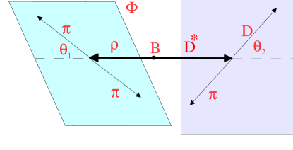
Figure 1: The angular distribution of the decay $B\to D^{*}\rho\to(D\pi)(\pi\pi)$

We consider a final state $f$, consisting of two vector mesons, to which both $B^{0}$ and ${\overline{B^{0}}}$ can decay. If only one weak amplitude contributes to $B^{0}\to f$ and ${\overline{B^{0}}}\to f$, we can write the helicity amplitudes as follows:

$$A_{\lambda}\equiv Amp(B^{0}\to f)_{\lambda} = a_{\lambda}e^{i\delta_{\lambda}^{a}}e^{i\phi_{a}}~{},$$ (4)

$$A^{\prime}_{\lambda}\equiv Amp({\overline{B^{0}}}\to f)_{\lambda} = b_{\lambda}e^{i\delta_{\lambda}^{b}}e^{i\phi_{b}}~{},$$ (5)

$${\bar{A}}^{\prime}_{\lambda}\equiv Amp(B^{0}\to{\bar{f}})_{\lambda} = b_{\lambda}e^{i\delta_{\lambda}^{b}}e^{-i\phi_{b}}~{},$$ (6)

$${\bar{A}}_{\lambda}\equiv Amp({\overline{B^{0}}}\to{\bar{f}})_{\lambda} = a_{\lambda}e^{i\delta_{\lambda}^{a}}e^{-i\phi_{a}}~{},$$ (7)

where the helicity index $\lambda$ takes the values $\left\{0,\|,\perp\right\}$. In the above, $\phi_{a,b}$ and $\delta^{a,b}_{\lambda}$ are the weak and strong phases, respectively.

Using CPT invariance, and the decay amplitude expressed in Eq. 3, the total decay amplitudes can be written as

$${\cal A}=Amp(B^{0}\to f)=A_{0}g_{0}+A_{\|}g_{\|}+i\,A_{\perp}g_{\perp}~{}~{},$$ (8)

$${\bar{\cal A}}=Amp({\overline{B^{0}}}\to{\bar{f}})={\bar{A}}_{0}g_{0}+{\bar{A}}_{\|}g_{\|}-i\,{\bar{A}}_{\perp}g_{\perp}~{}~{},$$ (9)

$${\cal A}^{\prime}=Amp({\overline{B^{0}}}\to f)=A^{\prime}_{0}g_{0}+A^{\prime}_{\|}g_{\|}-i\,A^{\prime}_{\perp}g_{\perp}~{}~{},$$ (10)

$${\bar{\cal A}}^{\prime}=Amp(B^{0}\to{\bar{f}})={\bar{A}}^{\prime}_{0}g_{0}+{\bar{A}}^{\prime}_{\|}g_{\|}+i\,{\bar{A}}^{\prime}_{\perp}g_{\perp}~{}~{},$$ (11)

where the $g_{\lambda}$ are the coefficients of the helicity amplitudes, defined using Eq. 3.

With the above equations, the time-dependent decay rate for a $B^{0}$ decaying into the two vector–meson final state, i.e. $B^{0}(t)\to f$, can be expressed as

$$\Gamma(B^{0}(t)\to f)=e^{-\Gamma t}\sum_{\lambda\leq\sigma} \Bigl{(}\Lambda_{\lambda\sigma}+\Sigma_{\lambda\sigma}\cos(\Delta Mt)$$ (12)

$$-\!\rho_{\lambda\sigma}\sin(\Delta Mt)\Bigr{)}g_{\lambda}g_{\sigma}\!~{}.$$

By performing a time-dependent study and angular analysis of the decay $B^{0}(t)\to\!f$, one can measure the 18 observables $\Lambda_{\lambda\sigma}$, $\Sigma_{\lambda\sigma}$ and $\rho_{\lambda\sigma}$. In terms of the helicity amplitudes $A_{0},A_{\|},A_{\perp}$, these can be expressed as follows:

$$\Lambda_{\lambda\lambda}=\displaystyle\frac{|A_{\lambda}|^{2}+|A^{\prime}_{\lambda}|^{2}}{2}, \Sigma_{\lambda\lambda}=\displaystyle\frac{|A_{\lambda}|^{2}-|A^{\prime}_{\lambda}|^{2}}{2},$$ (13)

$$\Lambda_{\perp i}=-\!{\rm Im}({A}_{\perp}{A}_{i}^{*}\!-\!A^{\prime}_{\perp}{A^{\prime}_{i}}^{*}), \Lambda_{\|0}={\rm Re}(A_{\|}A_{0}^{*}\!+\!A^{\prime}_{\|}{A^{\prime}_{0}}^{*}),$$

$$\Sigma_{\perp i}=-\!{\rm Im}(A_{\perp}A_{i}^{*}\!+\!A^{\prime}_{\perp}{A^{\prime}_{i}}^{*}), \Sigma_{\|0}={\rm Re}(A_{\|}A_{0}^{*}\!-\!A^{\prime}_{\|}{A^{\prime}_{0}}^{*}),$$

$$\rho_{\perp i}\!=\!-\!{\rm Re}\!\Bigl{(}\!\frac{q}{p}\![A_{\perp}^{*}A^{\prime}_{i}\!+\!A_{i}^{*}A^{\prime}_{\perp}\!]\!\Bigr{)}, \rho_{{\scriptscriptstyle\perp\perp}}\!=\!-\!{\rm Im}\Bigl{(}\frac{q}{p}\,A_{\perp}^{*}A^{\prime}_{\perp}\Bigr{)},$$

$$\rho_{\|0}\!=\!{\rm Im}\!\Bigl{(}\frac{q}{p}\![A_{\|}^{*}A^{\prime}_{0}\!+\!A_{0}^{*}A^{\prime}_{\|}\!]\!\Bigr{)}, \rho_{ii}\!=\!{\rm Im}\!\Bigl{(}\frac{q}{p}A_{i}^{*}A^{\prime}_{i}\Bigr{)},$$

where $i=\{0,\|\}$. In the above, $q/p=\exp({-2\,i\phi_{\scriptscriptstyle M}})$, where $\phi_{\scriptscriptstyle M}$ is the weak phase present in $B^{0}$–${\overline{B^{0}}}$ mixing.

Similarly, the decay rate for $B^{0}(t)\to{\bar{f}}$ is given by

$$\Gamma(B^{0}(t)\to{\bar{f}})=e^{-\Gamma t}\sum_{\lambda\leq\sigma} \Bigl{(}{\bar{\Lambda}}_{\lambda\sigma}+{\bar{\Sigma}}_{\lambda\sigma}\cos(\Delta Mt)$$ (14)

$$-{\bar{\rho}}_{\lambda\sigma}\sin(\Delta Mt)\Bigr{)}g_{\lambda}g_{\sigma}~{}.$$

The expressions for the observables ${\bar{\Lambda}}_{\lambda\sigma}$, ${\bar{\Sigma}}_{\lambda\sigma}$ and ${\bar{\rho}}_{\lambda\sigma}$ are similar to those given in Eq. (13), with the replacements $A_{\lambda}\to{\bar{A}}^{\prime}_{\lambda}$ and $A^{\prime}_{\lambda}\to{\bar{A}}_{\lambda}$.

With the above expressions for the various amplitudes, we now show how to extract weak phase information using the above measurements. First, we note that

$$\Lambda_{\lambda\lambda}={\bar{\Lambda}}_{\lambda\lambda}=\frac{(a_{\lambda}^{2}+b_{\lambda}^{2})}{2},\Sigma_{\lambda\lambda}=-{\bar{\Sigma}}_{\lambda\lambda}=\frac{(a_{\lambda}^{2}-b_{\lambda}^{2})}{2}.$$ (15)

Thus, one can determine the magnitudes of the amplitudes appearing in Eqs. (4)–(7), $a_{\lambda}^{2}$ and $b_{\lambda}^{2}$. However, it must be stressed that the knowledge of $b_{\lambda}^{2}$ will not be necessary within our method. This is important for the final states that have $b_{\lambda}\ll a_{\lambda}$, for which the determination of $b_{\lambda}^{2}$ would be very difficult.

Next, we have

$$\Lambda_{\perp i}\!=\!-{\bar{\Lambda}}_{\perp i}\!=\!b_{\perp}b_{i}\sin(\delta_{\perp}\!-\!\delta_{i}\!+\!\Delta_{i})-a_{\perp}a_{i}\sin(\Delta_{i}),$$

$$\Sigma_{\perp i}\!=\!{\bar{\Sigma}}_{\perp i}\!=\!-b_{\perp}b_{i}\sin(\delta_{\perp}\!-\!\delta_{i}\!+\!\Delta_{i})-a_{\perp}a_{i}\sin(\Delta_{i}),$$ (16)

where $\Delta_{i}\equiv\delta_{\perp}^{a}-\delta_{i}^{a}$ and $\delta_{\lambda}\equiv\delta_{\lambda}^{b}-\delta_{\lambda}^{a}$. Using Eq. (16) one can solve for $a_{\perp}a_{i}\sin\Delta_{i}$. We will see that this is the only combination needed to cleanly extract weak phase information.

The coefficients of the $\sin(\Delta mt)$ term, which can be obtained in a time-dependent study, can be written as

$$\rho_{\lambda\lambda}\!=\!\pm a_{\lambda}b_{\lambda}\sin(\phi\!+\!\delta_{\lambda}),{\bar{\rho}}_{\lambda\lambda}\!=\!\pm a_{\lambda}b_{\lambda}\sin(\phi\!-\!\delta_{\lambda}),$$ (17)

where the sign on the right hand side is positive for $\lambda=\|,0$, and negative for $\lambda=\perp$. In the above, we have defined the CP phase $\phi\equiv-2\phi_{\scriptscriptstyle M}+\phi_{b}-\phi_{a}$. These quantities can be used to determine

$$2b_{\lambda}\cos\delta_{\lambda}\!=\!\pm\frac{\rho_{\lambda\lambda}\!+\!{\bar{\rho}}_{\lambda\lambda}}{a_{\lambda}\sin\phi},2b_{\lambda}\sin\delta_{\lambda}\!=\!\pm\frac{\rho_{\lambda\lambda}\!-\!{\bar{\rho}}_{\lambda\lambda}}{a_{\lambda}\cos\phi}.$$ (18)

Similarly, the terms involving interference of different helicities are given as

$$\rho_{\perp i}\! = \!-a_{\perp}b_{i}\cos(\phi\!+\!\delta_{i}\!-\!\Delta_{i})\!-\!a_{i}b_{\perp}\cos(\phi\!+\!\delta_{\perp}\!+\!\Delta_{i}),$$

$${\bar{\rho}}_{\perp i}\! = \!-a_{\perp}b_{i}\cos(\phi\!-\!\delta_{i}\!+\!\Delta_{i})\!-\!a_{i}b_{\perp}\cos(\phi\!-\!\delta_{\perp}\!-\!\Delta_{i}).$$ (19)

Putting all the above information together, we are now in a position to extract the weak phase $\phi$. Using Eq. (18), the expressions in Eq. (19) can be used to yield

$$\!\rho_{\perp i}\!+\!{\bar{\rho}}_{\perp i}\!=-\cot\phi\,{a_{i}a_{\perp}}\cos\Delta_{i}\Bigg{[}\frac{\rho_{ii}+{\bar{\rho}}_{ii}}{a_{i}^{2}}-\frac{\rho_{\scriptscriptstyle\perp\perp}+{\bar{\rho}}_{{\scriptscriptstyle\perp\perp}}}{a_{\perp}^{2}}\Bigg{]}$$

$$~{}~{}~{}~{}~{}~{}~{}~{}~{}~{}~{}~{}-{a_{i}a_{\perp}}\sin\Delta_{i}\Bigg{[}\frac{\rho_{ii}-{\bar{\rho}}_{ii}}{a_{i}^{2}}+\frac{\rho_{{\scriptscriptstyle\perp\perp}}-{\bar{\rho}}_{{\scriptscriptstyle\perp\perp}}}{a_{\perp}^{2}}\Bigg{]},$$ (20)

$$\rho_{\perp i}\!-\!{\bar{\rho}}_{\perp i}=\tan\phi\,{a_{i}a_{\perp}}\cos\Delta_{i}\Bigg{[}\frac{\rho_{ii}-{\bar{\rho}}_{ii}}{a_{i}^{2}}-\frac{\rho_{\scriptscriptstyle\perp\perp}-{\bar{\rho}}_{{\scriptscriptstyle\perp\perp}}}{a_{\perp}^{2}}\Bigg{]}$$

$$~{}~{}~{}~{}~{}~{}~{}~{}~{}~{}~{}~{}-{a_{i}a_{\perp}}\sin\Delta_{i}\Bigg{[}\frac{\rho_{ii}+{\bar{\rho}}_{ii}}{a_{i}^{2}}+\frac{\rho_{{\scriptscriptstyle\perp\perp}}+{\bar{\rho}}_{{\scriptscriptstyle\perp\perp}}}{a_{\perp}^{2}}\Bigg{]}.$$ (21)

Now, we already know most of the quantities in the above two equations: (i) $\rho_{\lambda\sigma}$ and ${\bar{\rho}}_{\lambda\sigma}$ are measured quantities, (ii) the $a_{\lambda}^{2}$ are determined from the relations in Eq. (15), and (iii) ${a_{i}a_{\perp}}\sin\Delta_{i}$ is obtained from Eq. (16). Thus, the above two equations involve only two unknown quantities — $\tan\phi$ and ${a_{i}a_{\perp}}\cos\Delta_{i}$ — and can easily be solved (up to a sign ambiguity in each of these quantities). In this way $\tan^{2}\phi$ (or, equivalently, $\sin^{2}\phi$) can be cleanly obtained from the angular analysis.

Note that our method relies on the measurement of the interference terms between different helicities. However, we do not actually require that all three helicity components of the amplitude be used. In fact, one can use observables involving any two of largest helicity amplitudes. In the above description, one could have chosen ‘$\|\,0$’ instead of ‘$\perp\!\|$’ or ‘$\perp\!0$’.

We now turn to specific applications of this method. Consider first the situation in which the final state is a CP eigenstate, $f=\pm{\bar{f}}$. In this case, the parameters of Eqs. (4)–(7) satisfy $a_{\lambda}=b_{\lambda}$, $\delta_{\lambda}^{a}=\delta_{\lambda}^{b}$ (which implies that $\delta_{\lambda}=0$), and $\phi_{a}=-\phi_{b}$ (so that $\phi\equiv-2\phi_{\scriptscriptstyle M}+2\phi_{b}$). As described above, $a_{\lambda}^{2}$ can be obtained from Eq. 15. But now the measurement of $\rho_{\lambda\lambda}$ [Eq. (17)] directly yields $\sin\phi$. In fact, this is the conventional way of using the angular analysis to measure the weak phases: each helicity state separately gives clean CP-phase information. Thus, when $f$ is a CP eigenstate, nothing is gained by including the interference terms.

Of course, in general, final states that are CP eigenstates will all receive penguin contributions at some level. Thus, these states violate our assumption that only one weak amplitude contributes to $B^{0}\to f$ and ${\overline{B^{0}}}\to f$. The only quark-level decays which do not receive penguin contributions are ${\bar{b}}\to{\bar{c}}u{\bar{d}},~{}{\bar{u}}c{\bar{d}}$, as well as their Cabibbo-suppressed counterparts, ${\bar{b}}\to{\bar{c}}u{\bar{s}},~{}{\bar{u}}c{\bar{s}}$. Consider first the decays $B_{d}^{0}/{\overline{B_{d}^{0}}}\to D^{*-}\rho^{+},D^{*+}\rho^{-}$ In this case we have $\phi_{\scriptscriptstyle M}=\phi_{1}$, $\phi_{a}=0$ and $\phi_{b}=-\phi_{3}$, so that $\phi=-2\phi_{1}-\phi_{3}$. The method described above allows one to extract $\sin^{2}(2\phi_{1}+\phi_{3})$ from an angular analysis of the final state $D^{*\pm}\rho^{\mp}$.

In Ref. 6, Dunietz pointed out that $\sin^{2}(2\phi_{1}+\phi_{3})$ could, in principal, be obtained from measurements of $B_{d}^{0}(t)\to D^{\mp}\pi^{\pm}$. He used the method of Ref. 7, which requires the accurate measurement of the quantity $\Gamma({\overline{B_{d}^{0}}}\to D^{-}\pi^{+})/\Gamma(B_{d}^{0}\to D^{-}\pi^{+})$. This ratio is essentially $|V_{ub}V_{cd}^{*}/V_{cb}^{*}V_{ud}|^{2}\simeq 4\times 10^{-4}$. Obviously, it will be very difficult to measure this tiny quantity with any precision, which creates a serious barrier to carrying out Dunietz’s method in practice. On the other hand, our method does not suffer from this problem. In our notation [Eqs. (4)–(7)], the rate $\Gamma({\overline{B_{d}^{0}}}\to D^{*-}\rho^{+})$ is proportional to $b_{\lambda}^{2}$. However, as we have already emphasized in the discussion following Eq. (15), a determination of this quantity is not needed to extract $\sin^{2}(2\phi_{1}+\phi_{3})$ using the angular analysis: none of the observables or combinations required for the analysis are proportional to $b_{\lambda}^{2}$. Thus, we avoid the practical problems present in Dunietz’s method.

The two decay amplitudes for the final states $D^{*\pm}\rho^{\mp}$ have very different sizes, i.e. $b_{\lambda}\ll a_{\lambda}$. This results in a very small CP-violating asymmetry whose size is approximately $|V_{ub}V_{cd}^{*}/V_{cb}^{*}V_{ud}|\approx 2\%$. Thankfully, the situation is alleviated by the large branching ratio for the decay $B_{d}^{0}\to D^{*-}\rho^{+}$, roughly 1%. The Cabibbo-suppressed decays, e.g. $B_{d}^{0}\!\to\!{\bar{D}}^{*0}\!K^{*0}$, $D^{*0}K^{*0}$ and ${\overline{B_{d}^{0}}}\!\to\!D^{*0}{\bar{K}}^{*0}$, ${\bar{D}}^{*0}{\bar{K}}^{*0}$, with $K^{*0}$ and ${\bar{K}}^{*0}$ decaying to $K_{\scriptscriptstyle S}\pi^{0}$, lead to a larger asymmetry of about $|V_{ub}V_{cs}^{*}/V_{cb}^{*}V_{us}|\approx 40\%$. $\!{}^{{\bf?}}$ However, such Cabibbo-suppressed decays have much smaller branching ratios than those for $B_{d}^{0}/{\overline{B_{d}^{0}}}\to D^{*\pm}\rho^{\mp}$.

One can also consider $B_{s}^{0}$ and ${\overline{B_{s}^{0}}}$ decays. corresponding to the quark-level decays ${\bar{b}}\to{\bar{c}}u{\bar{d}},~{}{\bar{u}}c{\bar{d}}$, or ${\bar{b}}\to{\bar{c}}u{\bar{s}},~{}{\bar{u}}c{\bar{s}}$. The most promising processes are the Cabibbo-suppressed decay modes $B_{s}^{0}/{\overline{B_{s}^{0}}}\to D_{s}^{*\pm}K^{*\mp}$. Here the $B_{s}^{0}-{\overline{B_{s}^{0}}}$ mixing phase is almost $0$, so that the quantity $\sin^{2}\phi_{3}$ can be extracted from the angular analysis of $B_{s}^{0}(t)\to D_{s}^{*\pm}K^{*\mp}$. Other methods $\!{}^{{\bf?},{\bf?}}$ for obtaining the CP phase $\phi_{3}$ using similar final states have also been considered. $\!{}^{{\bf?}}$

It is even possible to cleanly extract the weak phase $\phi_{3}$ using only charged $B^{\pm}$ decays, $\!{}^{{\bf?}}$ by studying the angular distribution. The decays $B^{+}\to D^{*0}V^{+}$, $B^{+}\to\overline{D^{*0}}V^{+}$ and $B^{-}\to D^{*0}V^{-}$, $B^{-}\to\overline{D^{*0}}V^{-}$ can be related by CPT. Consider $D^{*0}/\overline{D^{*0}}$ decaying into $D^{0}\pi^{0}/\overline{D^{0}}\pi^{0}$, with $D^{0}/\overline{D^{0}}$ meson further decaying to a final state ‘$f$’ that is common to both $D^{0}$ and $\overline{D^{0}}$. $f$ is chosen to be a Cabibbo-allowed mode of $D^{0}$ or a doubly-suppressed mode of $\overline{D^{0}}$. The amplitudes for the decays of $B^{+}$ and $B^{-}$ to a final state involving $f$ will be a sum of the contributions from $D^{*0}$ and $\overline{D^{*0}}$, and similarly for the CP-conjugate processes. In this case one can experimentally measure the magnitudes of the 12 helicity amplitudes, as well as the interference terms, leading to a total of 24 independent observables. However, there are just 15 unknowns involved in the amplitudes: $a_{\lambda},b_{\lambda},\delta_{\lambda}^{a},\delta_{\lambda}^{b},\phi_{3},\Delta~{}{\rm and}~{}{\cal R}$; where, ${\cal R}^{2}=\frac{Br(\overline{D^{0}}\to f)}{Br(D^{0}\to f)},$ and $\Delta$ is the strong phase difference between $D^{0}\to f$ and $D^{0}\to{\overline{f}}$. Hence, the weak phase $\phi_{3}$ may be cleanly extracted.

The extraction of $\sin^{2}(2\phi_{1}+\phi_{3})$ may well turn out to be the second clean measurement to be made at $B$-factories. Studies are already underway for a possible measurement at the first generation B factory. $\!{}^{{\bf?}}$ The angle $\phi_{2}$ can be measured using an isospin analysis in $B_{d}^{0}\to\pi\pi$, $\!{}^{{\bf?}}$ but this technique requires measuring the branching ratio for $B_{d}^{0}\to\pi^{0}\pi^{0}$, which may be quite small. It is also possible to extract $\phi_{2}$ using a Dalitz-plot analysis of $B_{d}^{0}(t)\to\pi^{+}\pi^{-}\pi^{0}$ decays. $\!{}^{{\bf?}}$ It is estimated that this measurement will take roughly six years to complete. As for the angle $\phi_{3}$, the original suggestion using the decays $B^{\pm}\to D^{0}K^{\pm},~{}{\overline{D^{0}}}K^{\pm},~{}D^{0}_{\scriptscriptstyle CP}K^{\pm}$ $\!{}^{{\bf?}}$ runs into problems because it is virtually impossible to tag the flavor of the final-state $D$-meson. One can still obtain $\phi_{3}$ cleanly in other modes $\!{}^{{\bf?},{\bf?}}$ but this requires many more $B$’s, so that it is unlikely such measurements can be carried out in the first generation $B$-factories. Finally, there has been much work recently looking at the possibilities for extracting $\phi_{3}$ from $B\to\pi K$ decays. $\!{}^{{\bf?}}$ However, all of these methods use flavor $SU(3)$ symmetry, and so rely heavily on theoretical input. In view of all of this, it is conceivable that the second clean extraction of CP phases at $B$ factories will be the measurement of $\sin^{2}(2\phi_{1}+\phi_{3})$ using the method described here. We also note that the measurement of $\sin^{2}(2\phi_{1}+\phi_{3})$ may turn out to be very useful in looking for physics beyond the SM. For more details one is referred to Refs. 11 and 18.

To summarize, we have presented a new method of using an angular analysis in $B\to VV$ decay modes, which do not receive penguin contributions, to cleanly extract the weak phases $(2\phi_{1}+\phi_{3})$ and $\phi_{3}$. We have shown that the quantity $\sin^{2}(2\phi_{1}+\phi_{3})$ can be cleanly obtained from the time dependent angular analysis study of the decays $B_{d}^{0}(t)\to D^{*\pm}\rho^{\mp}$, $D^{*\pm}a_{1}^{\mp}$, $D^{*0}$${\scriptscriptstyle(}$–${\scriptscriptstyle)}$  $K^{*0}$${\scriptscriptstyle(}$–${\scriptscriptstyle)}$  , etc. Similarly, $\sin^{2}\phi_{3}$ can be cleanly extracted from $B_{s}^{0}(t)\to D_{s}^{*\pm}K^{*\mp}$, or simply performing an angular analysis of the decay mode $B^{\pm}\to\hbox{$D^{*0}$\kern-16.00008pt\raise 6.45831pt\hbox{{\raise 1.50696pt\hbox{${\scriptscriptstyle(}$}}--{\raise 1.50696pt\hbox{${\scriptscriptstyle)}$}}}}~{}~{}K^{*\pm}$ . Due to difficulties in measuring CP phases with other methods, $\sin^{2}(2\phi_{1}+\phi_{3})$ may well be the second clean measurement, after $\sin 2\phi_{1}$, to be measured at $B$-factories.

D.L. and R.S. would like to thank Prof. A. I. Sanda and the local organizers of BCP4 for financial support. We thank the organizers for an exciting conference. The work of D.L. was financially supported by NSERC of Canada.

References

References

[1] For a review, see H. Quinn and A. I. Sanda, Eur. Phys. J.C15, 626 (2000),
in The Review of Particle Physics, (Particle Data Group),
D.E. Groom et. al., Eur. Phys. J.C15, 1 (2000).
[2] D. London and R. Peccei, Phys. Lett.223B, 257 (1989); M.
Gronau, Phys. Rev. Lett.63, 1451 (1989), Phys. Lett.300B, 163 (1993); B. Grinstein,
Phys. Lett.229B, 280 (1989).
[3] I. Dunietz, H.R. Quinn, A. Snyder, W. Toki and H.J.
Lipkin, Phys. Rev.D43, 2193 (1991).
[4] N. Sinha and R. Sinha, Phys. Rev. Lett.80, 3706 (1998).
[5] A. S. Dighe I. Dunietz and R. Fleischer, Eur. Phys. J.C6, 647 (1999).
[6] I. Dunietz, Phys. Lett.427B, 179 (1998).
[7] R. Aleksan, I. Dunietz, B. Kayser and F. Le Diberder,
Nucl. Phys.B361, 141 (1991).
[8] For a discussion of CP violation in decays, see B. Kayser and D. London, Phys. Rev.D61: 116013 (2000).
[9] R. Aleksan, I. Dunietz and B. Kayser, Zeit. Phys.C54, 653 (1992).
[10]I. Dunietz and R. Fleischer, Phys. Lett.387B, 361 (1996).