LBNL-47750

CP-violation from Noncommutative Geometry

I. Hinchliffe and N. Kersting

Lawrence Berkeley National Laboratory, Berkeley, CA

If the geometry of space-time is $\rm noncommutative$, $\it i.e.$ $[x_{\mu},x_{\nu}]=i\theta_{\mu\nu}$, then $\rm noncommutative$ $CP~{}\rm{violating}$ effects may be manifest at low energies. For a $\rm noncommutative$ scale $\Lambda\equiv\theta^{-1/2}\leq 2~{}~{}TeV$, $CP~{}\rm{violation}$ from $\rm noncommutative~{}geometry$ is comparable to that from the Standard Model (SM) alone: the $\rm noncommutative$ contributions to $\epsilon$ and $\epsilon^{\prime}/\epsilon$ in the $K$-system, may actually dominate over the Standard Model contributions. Present data permit $\rm noncommutative~{}geometry$ to be the only source of $CP~{}\rm{violation}$. Furthermore the most recent findings for $g-2$ of the muon are consistent with predictions from $\rm noncommutative~{}geometry$.

1 Introduction

In recent years there has been a growing interest in quantum field theory over noncommutative spaces [1], that is spaces where the space-time coordinates $x_{\mu}$, replaced by hermitian operators $\widehat{x}_{\mu}$, do not commute:

$$[\widehat{x}_{\mu},\widehat{x}_{\nu}]=i\theta_{\mu\nu}$$ (1)

Here $\theta$ is a real and antisymmetric object with the dimensions of length-squared and corresponds to the smallest patch of area in physical space one may ’observe’, similar to the role $\hbar$ plays in $[\widehat{x_{i}},\widehat{p_{j}}]=i\hbar\delta_{ij}$, defining the corresponding smallest patch of phase space in quantum mechanics. In this paper we define the energy scale $\Lambda\equiv{1\over\sqrt{\theta}}$ (where $\theta$ is the average magnitude of an element of $\theta_{\mu\nu}$) which is a more convenient parameterization in constructing an effective theory at low energies. Many researchers set $\theta_{0i}=0$ to avoid problems with unitarity and causality, but since this is only an issue at energies above $\Lambda$ [2], we do not use this constraint for the purposes of low-energy phenomenology. We may view $\theta_{\mu\nu}$ as a “background $B$-field” which has attained a vacuum expectation value, hence appearing in the Lagrangian as a Lorentz tensor of constants [3]. Assuming that the components of $\theta_{\mu\nu}$ are constant over cosmological scales, in any given frame of reference there is a special “$\rm noncommutative$ direction” given by the vector $\theta^{i}\equiv\epsilon^{ijk}\theta_{jk}$. Experiments sensitive to $\rm noncommutative~{}geometry$ will therefore be measuring the components of $\overrightarrow{\theta}$, and it is necessary to take into account the motion of the lab frame in this measurement. Since $\rm noncommutative$ effects are measured in powers of $p^{\mu}\theta_{\mu\nu}p^{\prime\nu}$, where $p,p^{\prime}$ are some momenta involved in the measurement, it is possible that odd powers of $\theta$ will partially average to zero if the time scale of the measurement is long enough. Effects of first order in $\theta$ vanish at a symmetric $e^{+}e^{-}$-collider, for example, if the measurement averages over the entire $4\pi$ solid angle of decay products. If the data is binned by angle then it is possible to restore the sensitivity to $\theta$. In addition to any other averaging process over short time scales, terrestrial experiments performed over several days will only be sensitive to the projection of $\overrightarrow{\theta}$ on the axis of the Earth’s rotation. Of course binning the data hourly or at least by day/night, taking into account the time of year, can partially mitigate this effect. This axis, as well as the motion of the solar system, galaxy, $\it etc.$, does not vary over time scales relevant to terrestrial experiments.

The basic idea of $\rm noncommutative~{}geometry$ is not new and has been known in the context of string theory for some time [4]. We refer the reader to a few of the many excellent reviews of the mathematics of noncommutative space  [5, 6, 7, 8, 9] for a more rigorous understanding of the present material. Noncommuting coordinates are expected on quite general grounds in any theory that seeks to incorporate gravity into a quantum field theory: the usual semi-classical argument is that a particle may only be localized to within a Planck length $\lambda_{P}$ without creating a black hole that swallows the particle, hence $\sum_{i<j}{\Delta x_{i}\Delta x_{j}}\geq{\lambda_{P}}^{2}$; alternatively, one is led to think of space as a noncommutative algebra upon trying to quantize the Einstein theory [10, 11].

Much research has already gone into understanding noncommutative quantum field theory [12, 13, 14, 15]; it is equivalent to working with ordinary (commutative) field theory and replacing the usual product by the $\star~{}\rm{product}$ defined as follows:

$$(f\star g)(x)\equiv e^{i\theta_{\mu\nu}\partial_{\mu}^{y}\partial_{\nu}^{z}}f(y)g(z)\mid_{y=z=x}$$ (2)

With this definition (1) holds in function space equipped with a $\star~{}\rm{product}$:

$$[x_{\mu},x_{\nu}]_{\star}=i\theta_{\mu\nu}$$ (3)

This $\star~{}\rm{product}$ intuitively replaces the point-by-point multiplication of two fields by a sort of ’smeared’ product (see Fig. 1). Indeed the concept of ’smearing’ is borne out in more detailed analysis of 1- and 2- point functions [16]: spacetime is only well defined down to distances of order $\sqrt{\theta}$ so functions of spacetime must be appropriately averaged over a neighborhood of points. In each $(i,j)$ plane, we must replace

$$\phi(x_{i},x_{j})\rightarrow\int dx_{i}^{\prime}dx_{j}^{\prime}\phi(x^{\prime})e^{-\frac{(x_{i}-x_{i}^{\prime})^{2}+(x_{j}-x_{j}^{\prime})^{2}}{\theta_{ij}}}(\pi\theta_{ij})^{-1}$$ (4)

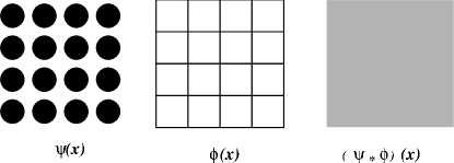
Figure 1: An illustration of the star product between two functions. The two scalar functions $\psi$ and $\phi$ are strongly orthogonal($\psi(x)\phi(x)=0~{}~{}\forall x$) yet the $\star~{}\rm{product}$ is nonzero.

Examples of theories which have received attention include scalar field theory [13, 17, 18], NCQED (the $\rm noncommutative$ analog of QED) [19], as well as noncommutative Yang-Mills [20, 21]; perturbation theory in $\theta$ is applicable and the theories are renormalizable [22, 23]. For gauge theories, a suitably adjusted definition of the gauge transformations  [24, 25] permits the construction of $SU(N)$ theories. There has been no work explicitly proving that fermion representations are consistent with such theories, however we know that the proof must exist since $\rm noncommutative~{}geometry$ is derived from a string theory which of course is self-consistent for all gauge groups and representations.

A $\rm noncommutative$ modification of the Standard Model(SM) is possible as a working field theory, at least up to ${\cal O}(\theta)$. Replacing the ordinary product with the $\star~{}\rm{product}$ in the Lagrangian, the appropriate Feynman rules for this $\rm noncommutative$ SM (ncSM) follow straightforwardly and are reproduced in the Appendix.

Whatever the physics at the Planck scale is like, we expect there to be some residual effect at low energies beyond that of classical gravity. If we parameterize this effect as in (1), then low energy physics will receive corrections in powers of the small parameter $\theta$. Several papers have addressed how these corrections may modify observations at an accelerator [26], precision tests of QED in hydrogen [27], and various dipole moments [28]; in general, if $\Lambda\leq 1~{}TeV$, there will be some observable effects in these systems at the next generation of colliders. This paper aims to investigate the $CP~{}\rm{violating}$ potential of $\rm noncommutative~{}geometry$ in low energy phenomenology.

2 Computing in the Noncommutative Standard Model(ncSM)

The method of computing $\rm noncommutative$ field theory amplitudes is effected by replacing the ordinary function product with the $\star~{}\rm{product}$ in the Lagrangian. The theory is otherwise identical to the commuting one (i.e. the Feynman path integral formulation provides the usual setting for doing QFT): for example a Yukawa theory with a scalar $\phi$, Dirac fermion $\psi$, has the action

$$S=\int{d^{4}x\left(\overline{\psi}i\hbox to0.0pt{\hbox to5.30904pt{\hfil/\hfil}\hss}\partial\psi+(\partial\phi)^{2}+\lambda\overline{\psi}\star\psi\star\phi\right)}$$ (5)

(Here we have used the fact that $\int{dx\xi\star\xi}=\int{dx\xi\xi}$, which follows straightforwardly from (2) ) Gauge interactions likewise generalize from the standard form; the action for NCQED for example is

$$S=\int{d^{4}x\left(-\frac{1}{4e^{2}}F^{\mu\nu}F_{\mu\nu}+\overline{\psi}i\hbox to0.0pt{\hbox to5.30904pt{\hfil/\hfil}\hss}\partial\psi-e\overline{\psi}\star\hbox to0.0pt{\hbox to7.50002pt{\hfil/\hfil}\hss}A\star\psi-m\overline{\psi}\psi\right)}$$ (6)

where

$$F_{\mu\nu}\equiv\partial_{\mu}A_{\nu}-\partial_{\nu}A_{\mu}-i[A_{\mu},A_{\nu}]_{\star}$$ (7)

Note the extra term in the field strength which is absent in ordinary QED; this nonlinearity gives NCQED a NonAbelian-like structure. There will be, for example, 3- and 4-point photon self-couplings at tree level (see Appendix).

In momentum space the $\star~{}\rm{product}$ becomes a momentum-dependent phase factor which means that the theory effectively contains an infinite number of derivative interactions suppressed by powers of $\theta$. This directly exhibits the nonlocal character of $\rm noncommutative~{}geometry$. From (5) and (6) we can derive the action for the $\rm noncommutative$ version of the Standard Model (ncSM). We present its content as the list of Feynman rules in the Appendix.

A central feature of computations in the SM is the presence of divergences and the need to absorb them into counterterms. The ncSM is similar in this respect, yet it is necessary to renormalize carefully: if one simply uses dimensional regularization and sums virtual energies to infinity, bizarre infrared singularities appear in the theory which are difficult to handle [13]. To illustrate, consider the loop integral

$$\int{d^{d}k\frac{e^{ik^{\mu}\theta_{\mu\nu}p^{\nu}}}{(k^{2}-m^{2})^{2}}}$$ (8)

which is finite for $\left|\theta\cdot p\right|\neq 0$ but is logarithmically divergent if $\left|\theta\right|=0$. Explicitly, we Wick-rotate (8), introduce the Schwinger parameters [29], integrate over momenta, and obtain

$$\int{dS~{}S^{1-{d\over 2}}~{}e^{-\frac{1}{4}(\theta\cdot p)^{2}S^{-1}-m^{2}S}}$$ (9)

If we take $\left|\theta\right|=0$ now, dimensional regularization gives the usual $\Gamma[1-{d\over 2}]$ which we would absorb into a counterterm of the theory. However for small finite values of $\left|\theta\cdot p\right|$ we get an approximation of the integral (9) in four dimensions:

$$\int{d^{4}k\frac{e^{ik^{\mu}\theta_{\mu\nu}p^{\nu}}}{(k^{2}-m^{2})^{2}}}\approx ln(m^{2}\left|\theta\cdot p\right|^{2})\left(1+m^{2}\left|\theta\cdot p\right|^{2}\right)$$ (10)

There is a $ln(\left|\theta\right|)$ divergence as $\left|\theta\right|\to 0$ which is expected since in this limit the theory tends to the commutative one and reproduces the $\Gamma[1-{d\over 2}]$ divergence mentioned above. This is formally correct, however the theory in this limit is awkward to work with since some contributions will diverge as $\left|\theta\right|\to 0$ and must produce final results such as scattering amplitudes which are finite. For the computational purposes of this paper, in which $\it e.g.$ ${m_{W}}^{2}\left|\theta\right|\ll 1$, it is more convenient to regularize with a Pauli-Vilars regulator with mass $M$. Then (9) becomes

$$\int{dS~{}S^{1-{d\over 2}}~{}e^{-(M^{-2}+\frac{1}{4}(\theta\cdot p)^{2})S^{-1}-m^{2}S}}$$ (11)

Taking the limit $\left|\theta\right|\to 0$ now gives

$$\int{d^{d}k\frac{e^{ik^{\mu}\theta_{\mu\nu}p^{\nu}}}{(k^{2}-m^{2})^{2}}}\approx ln(\frac{m^{2}}{M^{2}}+m^{2}\left|\theta\cdot p\right|^{2})+m^{2}\left|\theta\cdot p\right|^{2}ln(\frac{m^{2}}{M^{2}}+m^{2}\left|\theta\cdot p\right|^{2})$$ (12)

Note that in the limit $\left|\theta\right|\to 0$ the second term vanishes while the first term reproduces the ordinary(commutative) loop integral divergence. We subtract this into a counterterm, while the remaining piece gives a small correction to the commutative theory of ${\cal O}(x~{}ln(x))$ where $x\equiv\left|m~{}\theta\cdot p\right|^{2}$. Renormalizing in this manner guarantees sensible results.

3 CP Violation in the ncSM

In the SM, there are only two sources of $CP~{}\rm{violation}$: the irremovable phases in the CKM matrix and the $\Theta F\tilde{F}$ term in the strong interaction Lagrangian(the coefficient $\Theta$ has to be miniscule to avoid contradicting experiment [30]).

In the ncSM, there is an additional source of $CP~{}\rm{violation}$: the parameter $\theta$ itself is the $CP~{}\rm{violating}$ object, which is apparent from the NCQED action (6) considering the transformation of $A_{\mu}$ and $\partial_{\mu}$ under $C$ and $P$ and assuming $CPT$ invariance [31]. Physically speaking, an area of ${\cal O}(\theta)$ represents a “black box” in which some or all spacetime coordinates become ambiguous, which in turn leads to an ambiguity between particle and antiparticle. More detailed work reveals that $\theta$ is in fact proportional to the size of an effective particle dipole moment [32]. Therefore $\rm noncommutative~{}geometry$ can actually explain the origin of $CP~{}\rm{violation}$. At the field theory level, it is the momentum-dependent phase factor appearing in the $\rm noncommutative$ theory which gives $CP~{}\rm{violation}$. For example, the ncSM W-quark-quark $SU(2)$ vertex in the flavor basis is

$${\cal L}_{Wqq}=\overline{u(p)}\gamma^{\mu}(1-\gamma_{5})e^{ip\cdot\theta\cdot p^{\prime}}~{}d(p^{\prime})~{}W_{\mu}$$ (13)

Once we perform rotations on the quark fields to diagonalize the Yukawa interactions, $\it i.e.$ $u_{L}\to Uu_{L}$ and $d_{L}\to Vd_{L}$, the above becomes

$${\cal L}_{Wqq}=\overline{u(p)}\gamma^{\mu}(1-\gamma_{5})e^{ip\cdot\theta\cdot p^{\prime}}U^{\dagger}V~{}d(p^{\prime})~{}W_{\mu}$$ (14)

Even if $U^{\dagger}V$ is purely real, there will be some nonzero phases $e^{ip\cdot\theta\cdot p^{\prime}}$ in the Lagrangian whose magnitudes increase as the momentum flow in the process increases. Of course, the above phase factor has no effect at tree-level (suitably redefining all the fields) but will affect results at 1-loop and beyond.

Experimentally, the signal for $\rm noncommutative~{}geometry$ here is a momentum-dependent CKM matrix (ncCKM) which we define as follows:

$$\overline{V}(p,p^{\prime})\equiv\left(\begin{array}[]{ccc}1-\lambda^{2}/2+ix_{ud}&\lambda+i\lambda x_{us}&A\lambda^{3}(\rho-i\eta)+iA\lambda^{3}\rho x_{ub}\\ -\lambda-i\lambda x_{cd}&1-\lambda^{2}/2+ix_{cs}&A\lambda^{2}+iA\lambda^{2}x_{cb}\\ A\lambda^{3}(1-\rho-i\eta)+iA\lambda^{3}\rho x_{td}&-A\lambda^{2}-A\lambda^{2}ix_{ts}&1+ix_{tb}\\ \end{array}\right)$$ (15)

where $x_{ab}\equiv{p_{a}}^{\mu}\theta_{\mu\nu}{p^{\prime}_{b}}^{\nu}$ for quarks $a,b$. This matrix is an approximation of the exact ncSM in the perturbative limit where we expand $e^{ip\cdot\theta\cdot p^{\prime}}\approx 1+ip\cdot\theta\cdot p^{\prime}$ . In the limit $\theta\to 0$, the $x_{ab}$ all go to zero and $\overline{V}$ becomes the CKM matrix $V$ in the Wolfenstein parameterization [33] in terms of the small number $\lambda\approx 0.22$. Note that $\overline{V}$ is not guaranteed to be unitary, since, in contrast to the SM CKM matrix, $\overline{V}$ is not a collection of derived constants: a given matrix element will attain different values depending on the process it is describing. As an example, suppose we measure a non-zero $\tau$-polarization asymmetry in $t\to b\tau^{+}\nu$ [34]; this puts a constraint on the value of $\Im(\overline{V}_{tb})$ at the energy scale $\mu\approx m_{t}$. We can get another constraint on $\Im(\overline{V}_{tb})$ through a $B^{0}-\overline{B}^{0}$ oscillation experiment, but we must take into consideration that this is a measurement at the energy scale $\mu\approx m_{b}$. In the former process we would find (for $\eta=0$) $\Im(\overline{V}_{tb})\approx{\cal O}({m_{t}}^{2}\left|\theta\right|)$ whereas in the latter it would be ${\cal O}(m_{t}m_{b}\left|\theta\right|)$, so these phases differ by a factor of $m_{t}/m_{b}\approx 30$. Therefore we expect the phenomenology of $\overline{V}$ to be rather different from that of the SM. In addition to $CP~{}\rm{violation}$ from the weak interaction (in $\overline{V}$), there will also be $CP~{}\rm{violation}$ from the strong and electromagnetic interactions (since there are phases entering any vertex with three (or more) fields (see Appendix)). We now turn to the phenomenological implications of these.

3.1 CP Violating Observables

3.1.1 $\epsilon_{K}$

The $CP~{}\rm{violating}$ observable of choice in the $K^{0}$-meson system is $\epsilon_{K}$ which is directly proportional to the imaginary part $\Im(M_{12})$ of the box graph (see Fig. 2):

$$\epsilon_{K}\equiv\frac{\Im(M_{12})}{\Delta m}$$ (16)

The mass splitting $\Delta m$ between the long- and short-lived $K^{0}$ eigenstates
is $\Delta m\approx 3.5\cdot 10^{-15}~{}GeV$ [36]. We can rewrite

$$\Im(M_{12})=\frac{{G_{F}}^{2}{m_{W}}^{2}{f_{K}}^{2}B_{K}m_{K}}{12\pi^{2}}\Im(loop)$$ (17)

in terms of the decay constants $f_{K},B_{K}$, and the loop factor. In the SM, the loop factor is

$$\Im(loop)\approx\Im({\lambda_{c}}^{2}f(m_{c})+{\lambda_{t}}^{2}f(m_{t})+\lambda_{c}\lambda_{t}f(m_{c},m_{t}))$$ (18)

Figure 2: The box graph for $K^{0}$-$\overline{K^{0}}$ mixing in the Standard Model with exchange of virtual $W$-bosons and up-type quarks from the $i,j$ generations.

where $\lambda_{q}\equiv V_{qd}V_{qs}^{*}$ and $f(x)$ is a loop function (see Appendix). In the SM, both charm and top quarks contribute roughly equally to the imaginary part of the loop, and the measured value for $\epsilon_{K}$ puts a constraint on the parameters $\rho,\eta$ of the CKM matrix. However, in the ncSM we must replace the entire loop since the momentum-dependent phases in $\overline{V}$ change how the loop integral behaves. Note the charm quark will dominate the imaginary part of the graph because the phase of the product $(\overline{V}_{ts}^{*}\overline{V}_{td})^{2}$ is a factor of $\lambda^{8}$ suppressed relative to the phase of $(\overline{V}_{cs}^{*}\overline{V}_{cd})^{2}$ (see (15)). We record the evaluation of the loop integral in the Appendix.

If the kaons used in the measurement emerge from a beam with an average velocity $\beta\equiv{v\over c}$ in the lab frame, we must average over the motion of the internal constituents of the kaon, since the entire $\rm noncommutative$ effect is proportional to $p\cdot\theta\cdot p^{\prime}$, where $p,p^{\prime}$ are the momenta of the constituents. We assume that these momenta have random orientation in the rest frame of the kaon, subject to $p+p^{\prime}=(m_{K},0,0,0)$. The average over these internal momenta produces a result which is proportional to the velocity of the kaon in the lab frame: $\langle p\cdot\theta\cdot p^{\prime}\rangle\approx\left|\theta\right|\beta\gamma~{}m_{K}^{2}$. Therefore it is important that the $\beta\gamma$ of the beam not be so small as to wash out the signal. Recent determinations of $\epsilon_{K}$ use a reasonable $\beta\gamma$ [37], so we do not concern ourselves further with this caveat. Experiments at an $e^{+}e^{-}$ collider ($\it e.g.$ [38, 39]) where the center of mass is stationary in the lab frame should, however, see no signal for $\epsilon_{K}$ since $\langle\overrightarrow{\beta}\gamma\rangle=0$. As we mentioned in the Introduction, the data may be sensitive to the time of day. If there is a component of $\overrightarrow{\theta}$ along the axis of the Earth, then given enough statistics there should be a “day/night effect” for $\epsilon_{K}$ which, as far as we know, no experiment has looked for.

In the case $\eta=0$ (so the phase from $\overline{V}$ is due entirely to $\rm noncommutative~{}geometry$), we obtain

$$\begin{array}[]{l}\epsilon_{K}\approx\frac{{G_{F}}^{2}{m_{W}}^{2}{f_{K}}^{2}B_{K}m_{K}}{12\pi^{2}\Delta m}\lambda^{2}\frac{m_{K}}{m_{W}}\xi^{2}\\ \\ \xi\equiv\frac{m_{W}}{\Lambda}\end{array}$$ (19)

Using $G_{F}=1.166\cdot 10^{-5}~{}GeV^{-2},m_{W}=80.4~{}GeV,f_{K}=0.16~{}GeV,m_{K}=0.498~{}GeV,B_{K}=0.70\pm 0.2,\rho=0.3\pm 0.2$, and the latest measurement of $\epsilon_{K}\approx(2.280\pm 0.013)\cdot 10^{-3}$ [36], this implies $\xi\approx(4\pm 2)\cdot 10^{-2}$ (see Fig. 3); in this scenario spacetime becomes effectively $\rm noncommutative$ at energies above $\approx 2~{}TeV$.

Figure 3: Variation of $\epsilon$ with $\xi\equiv m_{W}/\Lambda$. Here $\eta=0$ so all $CP~{}\rm{violation}$ is from $\rm noncommutative~{}geometry$.

3.1.2 $\epsilon^{\prime}/\epsilon$

Direct $CP~{}\rm{violation}$ is measurable in the neutral kaon system as a difference between the rates at which $K_{L,S}$ decay into $I=0,2$ states of pions:

$$\epsilon^{\prime}\equiv\frac{\langle 2\mid T\mid K_{L}\rangle\langle 0\mid T\mid K_{S}\rangle-\langle 2\mid T\mid K_{S}\rangle\langle 0\mid T\mid K_{L}\rangle}{\sqrt{2}\langle 0\mid T\mid K_{S}\rangle^{2}}$$ (20)

Then the ratio of direct to indirect $CP~{}\rm{violation}$ is

$$\frac{\epsilon^{\prime}}{\epsilon}=\frac{1}{\sqrt{2}}\left(\frac{\langle 2\mid T\mid K_{L}\rangle}{\langle 0\mid T\mid K_{L}\rangle}-\frac{\langle 2\mid T\mid K_{S}\rangle}{\langle 0\mid T\mid K_{S}\rangle}\right)$$ (21)

The theoretical computation of this ratio is a challenge in the SM not only because the perturbative description of the strong interaction is not reliable at low energies but also because it is proportional to a difference between two nearly equal contributions, enhancing the theoretical error [40]. The most naive way to estimate $\frac{\epsilon^{\prime}}{\epsilon}$ employs the so-called vacuum-saturation-approximation (VSA) which is based on the factorization of four-quark operators into products of currents and the use of the vacuum as an intermediate state (for more details see [41]). The estimate is

$$\frac{\epsilon^{\prime}}{\epsilon}\approx(0.8\pm 0.5)\cdot 10^{-3}\left(\frac{\Im(\lambda_{t})}{10^{-4}}\right)$$ (22)

where in the SM $\lambda_{t}$ represents the $CP~{}\rm{violating}$ phases from the CKM matrix, $\lambda_{t}=A^{2}\lambda^{5}\eta\approx 1.3\cdot 10^{-4}$. The experiments measure $\frac{\epsilon^{\prime}}{\epsilon}=(1.92\pm 0.46)\cdot 10^{-3}$ which does not closely match the VSA number, but it is possible to use more elaborate models that agree closely with the measured value [40].

In the ncSM it is no less difficult to compute $\frac{\epsilon^{\prime}}{\epsilon}$; in particular, the extra phases from
$\rm noncommutative~{}geometry$ will become involved in the complicated nonperturbative quark-gluon dynamics. The best estimate we can make here is (see Appendix C)

$$\Im(\lambda_{t})\approx 2\frac{m_{K}}{m_{W}}\xi^{2}~{}ln(\frac{m_{W}}{\xi m_{K}})$$ (23)

For $\xi\approx 0.04$, we get roughly the same VSA value as in the SM.

3.1.3 $sin2\beta$ and the unitarity triangle

The only $CP~{}\rm{violating}$ observation from the $B$-system to date, the asymmetry in the decay products of $B^{0}\to J/\psi{K_{s}}^{0}$  [42, 43, 44, 45], is a measurement in the SM of a combination of CKM elements called $sin2\beta$:

$$sin2\beta\equiv\Im\left(-\left[\frac{V_{tb}^{*}V_{td}}{V_{tb}V_{td}^{*}}\right]\left[\frac{V_{cs}^{*}V_{cb}}{V_{cs}V_{cb}^{*}}\right]\left[\frac{V_{cd}^{*}V_{cs}}{V_{cd}V_{cs}^{*}}\right]\right)$$ (24)

where the first bracketed factor is from ${B_{d}}^{0}-\overline{B_{d}}^{0}$ mixing, the second from the observed decay asymmetry, and the third from ${K}^{0}-\overline{K}^{0}$ mixing. In the Wolfenstein parameterization,

$$sin2\beta\approx\frac{2\eta(1-\rho)}{\eta^{2}+(1-\rho)^{2}}$$ (25)

which, for $(\rho,\eta)\approx(0.2,0.3)$, corresponding to a point in the center of the allowed region of the $\rho-\eta$ plane [46] implies $sin2\beta\approx 0.7$. The most recent experimental world average for this quantity is $\approx 0.49\pm 0.23$ [47].

In the ncSM the corresponding quantity is (24) with each matrix element $V_{ij}$ replaced by $\overline{V}_{ij}$ extracted from the relevant process:

$$sin2\beta\to\Im\left(-\left[\frac{\overline{V}_{tb}^{*}\overline{V}_{td}}{\overline{V}_{tb}\overline{V}_{td}^{*}}\right]\left[\frac{\overline{V}_{cs}^{*}\overline{V}_{cb}}{\overline{V}_{cs}\overline{V}_{cb}^{*}}\right]\left[\frac{\overline{V}_{cd}^{*}\overline{V}_{cs}}{\overline{V}_{cd}\overline{V}_{cs}^{*}}\right]\right)$$ (26)

Of course experiments don’t measure the precise value of a given $\overline{V}_{ij}$ but rather some combination of them integrated over internal momenta. If we again consider the scenario where $\eta=0$ then the imaginary parts of these quantities increase roughly proportionally to the momenta involved and we expect the first bracketed term in (26) to dominate since the size of the momenta involved in ${B_{d}}^{0}-\overline{B_{d}}^{0}$ mixing exceeds that of $B^{0}$-decay or ${K}^{0}-\overline{K}^{0}$ mixing, $\it i.e.$ $m_{b}m_{t}\theta\gg m_{b}^{2}\theta,m_{K}m_{t}\theta$. We therefore set the second and third brackets to unity, obtaining

$$sin2\beta\approx\Im\left(\frac{1-ix_{tb}}{1+ix_{tb}}\right)\approx\frac{m_{b}}{m_{W}}\xi^{2}$$ (27)

If we use the measurement of $\epsilon_{K}$ to fix $\xi\approx 10^{-2}$, then the ncSM predicts $sin2\beta\approx 0$ which is not excluded by experiment. The motion of the quarks inside the $B$-meson moreover partially washes out the signal (see previous discussion for kaons) as the asymmetry of the $e^{+}e^{-}$ collider gives the ${B_{d}}^{0}-\overline{B_{d}}^{0}$ center-of-mass only a modest boost of $\beta\gamma\approx 0.6$ in the lab frame. We conclude that this model predicts that current $B$-physics experiments should see a value of $sin2\beta$ which is consistent with zero.

The other two $CP~{}\rm{violating}$ observables commonly defined in $B$-physics are $\alpha$ and $\gamma$:

$$\alpha\equiv arg\left(-\frac{V_{tb}^{*}V_{td}}{V_{ud}V_{ub}^{*}}\right)~{}~{}~{}~{}~{}~{}~{}~{}~{}~{}~{}~{}~{}~{}~{}~{}~{}~{}~{}~{}~{}\gamma\equiv arg\left(-\frac{V_{cd}^{*}V_{cb}}{V_{ud}V_{ub}^{*}}\right)$$ (28)

where $V_{tb}^{*}V_{td}$ can be extracted from ${B_{d}}^{0}-\overline{B_{d}}^{0}$ mixing and $V_{ud}V_{ub}^{*}$, $V_{cd}^{*}V_{cb}$ from neutral and charged $B$-decays such as $B^{0}\to\pi\pi$ and $B^{+}\to\pi^{+}K^{0}$, for example. In the SM $\alpha+\beta+\gamma=\pi$ because the CKM matrix $V$ is unitary. The ncSM matrix $\overline{V}$ is not unitary (see Section 3), so we expect $\alpha+\beta+\gamma\neq\pi$ as these “angles” are defined (by $\overline{V}$ replacing $V$ in (28) above). For $\eta=0$ the parameters $\alpha,\beta,\gamma$ in the ncSM assume the following form:

$$\begin{array}[]{l}\alpha\approx tan^{-1}\left(\frac{m_{b}}{m_{W}}\xi^{2}\right)\\ \beta\approx tan^{-1}\left(\frac{m_{b}+m_{K}}{m_{W}}\xi^{2}\right)\\ \gamma\approx\pi-tan^{-1}\left(\frac{m_{K}}{m_{W}}\xi^{2}\right)\\ \end{array}$$ (29)

In Figure 4 we plot the sum $\alpha+\beta+\gamma$. The angles essentially add up to $\pi$ in the same range of $\xi$ which is required by the $\epsilon_{K}$-constraint. If all the matrix elements of $\overline{V}$ could be measured at the same energy then the unitarity triangle would close exactly. The small deviation from exact closure is ${\cal O}(\frac{m_{b}}{m_{W}}\xi^{2})$ and represents the fact that the angles as defined in (26) and (28) are a combination of amplitudes measured at different energies: $\mu\sim m_{t}$ (for ${B_{d}}^{0}-\overline{B_{d}}^{0}$ mixing) and and $\mu\sim m_{b}$ (for $B$ decays).

Figure 4: Plot of the difference $\alpha+\beta+\gamma-\pi$ in the ncSM illustrating that the unitarity triangle does not close exactly.

3.1.4 Electric Dipole Moments

Nonzero values of the electric dipole moments ($\it edm$s) of the elementary fermions necessarily violate $T$, and hence $CP$ (assuming the $CPT$ theorem). This follows from the observation that a dipole moment $\overrightarrow{D}$ is a directional quantity, so for an elementary particle it must transform like the spin $\overrightarrow{J}$, the only available directional quantum number. The interation with an external electric field $\overrightarrow{E}$ is $\overrightarrow{J}\cdot\overrightarrow{E}$ which is therefore $CP$-odd. The presence of an $\it edm$ for a particle $\psi$ implies an interaction with the electromagnetic field strength $F^{\mu\nu}$ in the Lagrangian of the form

$$O_{edm}=-(i/2)\overline{\psi}\gamma_{5}\sigma_{\mu\nu}\psi F^{\mu\nu}$$

In the SM this operator is absent at tree level and even at one loop due to a cancellation of the CKM phases. For the electron, moreover, the $\it edm$ ($d_{e}$) vanishes at two loops and the three-loop prediction is miniscule, of order $10^{-50}e~{}cm$ [48]. For the neutron $\it edm$ ($d_{n}$), gluon interactions can give rise to a two-loop contribution which is ${\cal O}(10^{-33})e~{}cm$. Upper limits from experiments exist: $d_{e}\leq 4.3\cdot 10^{-27}e~{}cm$ [49], $d_{n}\leq 6.3\cdot 10^{-26}e~{}cm$ [50].

Since the SM predictions of $\it edm$s are almost zero, we might expect that new sources of $CP~{}\rm{violating}$ physics from $\rm noncommutative~{}geometry$ would be observable. The noncommutative geometry provides in addition a simple explanation for this type of $CP~{}\rm{violation}$: the directional sense of $\overrightarrow{D}$ derives from the different amounts of noncommutivity in different directions ($\it i.e.$ $D_{i}\propto\epsilon_{ijk}\theta^{jk}$) and the size of the $\it edm$, classically proportional to the spatial extent of a charge distribution, is likewise in $\rm noncommutative~{}geometry$ proportional to $\left|\theta\right|$, the inherent “uncertainty” of space. The effects of $\rm noncommutative~{}geometry$ will be proportional to the typical momentum involved, which for an electron $\it edm$ observation is $\sim keV$. A detailed analysis of the size of the $\it edm$ appears in  [28], but a simple estimate of the expected dipole moment is

$$d_{e}\sim e\left|p\theta\right|\approx 10^{-20}(\frac{p_{e}}{1~{}keV})\xi^{2}~{}e\cdot cm$$ (30)

which gives an apparently strong upper bound: $\xi<10^{-3}$. Although the phenomenologically interesting values of $\xi$ from the $K$-sector is well above this bound, we cannot exclude the possibility that the actual $\it edm$ is much smaller than the above naive estimate, a situation which can arise in supersymmetric models  [51, 52].

4 Constraints from $\bf{g-2}$ of the Muon

Since $\rm noncommutative$ effects are proportional to momentum, we might expect an even stronger constraint by considering the muon $\it edm$ in an experiment using relativistic muons, however the experimental bound here is weaker: $d_{\mu}<1.05\cdot 10^{-18}e~{}cm$ [53].

The recent measurement of the anomalous magnetic moment of the muon [54], $a_{\mu}$, although not a $CP~{}\rm{violating}$ observable, does however provide an interesting constraint on the ncSM. Experiments dedicated to $a_{\mu}$ have undergone continual refinement (for history and experimental details, see [53], [55]) to the point where $a_{\mu}$ is now very precisely known:

$$a_{\mu}^{expt}=11659202(14)\cdot 10^{-10}$$ (31)

The experimental technique employs muons trapped in a storage ring. A uniform magnetic field $B$ is applied perpendicular to the orbit of the muons; hence the muon spin will precess. The signal is a discrepancy between the observed precession and cyclotron frequencies.

Precession of the muon spin is determined indirectly from the decay $\mu\to e~{}{\overline{\nu}}_{e}~{}\nu_{\mu}$. Electrons emerge from the decay vertex with a characteristic angular distribution which in the SM has the following form in the rest frame of the muon:

$$dP(y,\phi)=n(y)(1+A(y)cos(\phi))dyd(cos(\phi))$$ (32)

where $\phi$ is the angle between the momentum of the electron and the spin of the muon, $y=2p_{e}/m_{\mu}$ measures the fraction of the maximum available energy which the electron carries, and $n(y),A(y)$ are particular functions which peak at $y=1$. The detectors (positioned along the perimeter of the ring) accept the passage of only the highest energy electrons in order to maximize the angular asymmetry in (32). In this way, the electron count rate is modulated at the frequency $a_{\mu}eB/(2\pi mc)$.

Although $a_{\mu}$ does receive a sizable contribution from $\rm noncommutative~{}geometry$, it is a constant contribution [28], $\it i.e.$ the interaction with the external magnetic field $\Delta E\sim B_{i}\theta_{jk}\epsilon^{ijk}$ is independent of the muon spin, and therefore the experiment described above is not sensitive to this perturbation of $a_{\mu}$. The effect of $\rm noncommutative~{}geometry$ on this measurement does however enter in the manner in which the muon spin is measured in its decay. Specifically, the electron decay distribution (32) has a slightly different angular dependence due to the departure of the ncSM from the standard V-A theory of the weak interactions (see Figure 5). The electron distribution $dP^{\prime}$ in the ncSM differs from the SM (we reserve the details for a future publication):

$$\begin{array}[]{ll}dP^{\prime}(y,\phi)&\approx n(y)\left(1+A(y)(\overrightarrow{p_{e}}\cdot\overrightarrow{s}_{\mu})+f(y)(\hat{p}_{e}\cdot\theta\cdot\overrightarrow{s}_{\mu})(\overrightarrow{p_{e}}\cdot\overrightarrow{s}_{e})+\cdot\cdot\cdot\right)dyd\Omega\\ &\to n(1)\left(1+A(1)cos(\phi)+f(1)sin(2\phi)\left|\theta\right|+\cdot\cdot\cdot\right)dyd\Omega\\ \\ {\rm where}&\left|{f(1)\over A(1)}\right|\approx\frac{\alpha}{16\pi^{2}}\frac{p_{\mu}}{m_{W}}\xi\\ \end{array}$$ (33)

The effect of $\rm noncommutative~{}geometry$ is greater than one would naively expect as, for reasons of efficiency, the muons are stored at highly relativistic energies: $p_{\mu}\approx 3~{}GeV$. Hence the ratio $\left|{f(1)\over A(1)}\right|\approx 10^{-6}\xi$. However, the frequency is measured over many cycles and a more conservative estimate of the effective size of the $\rm noncommutative$ term is closer to $(10^{-7}~{}to~{}10^{-8})\xi$ The angular distribution is therefore not a pure $cos(\phi)$ and we expect the measurement of the precession frequency to differ from the SM prediction at the level of 1 part in $10^{8}$.

Currently, the discrepancy between the measured value of $a_{\mu}$ and the SM prediction is

$$a_{\mu}^{expt}-a_{\mu}^{SM}=43(16)\cdot 10^{-10}$$ (34)

which imposes the constraint $\xi\leq 5\cdot 10^{-2}$. This bound accomodates the values of $\xi$ inferred from $CP~{}\rm{violating}$ observables in section 3.1. We expect the value of $\xi$ determined from a $g-2$ experiment to be smaller than that from a $K$ or $B$-physics experiment since the circulation of the muons at their cyclotron frequency introduces an additional averaging of the components of $\overrightarrow{\theta}$. For a storage ring located at an Earth lattitude of $\psi$ degrees, there will be a $sin(\psi)$ suppression factor.

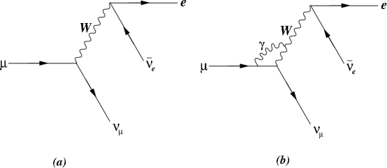
Figure 5: Contributions to muon decay (a) SM tree level (b) ncSM graph which upsets the electron’s angular distribution

5 Conclusions

The Standard Model(SM) is a highly successful effective theory for energies below the weak scale $\sim 100~{}GeV$, but it must eventually give way to a description of nature that includes gravity. Noncommutative geometry is one candidate for such a description, exhibiting some features of gravity such as nonlocality and space-time uncertainty.

In this paper we have considered the potential effects at low eneriges of a noncommutative geometry which sets in at some high scale $\Lambda$. Remarkably, for $\Lambda$ in the $TeV$- range, $\rm noncommutative$ contributions to $CP~{}\rm{violating}$ observables such as $\epsilon_{K}$ and $\epsilon^{\prime}/\epsilon$ are competitive with the SM contributions, whereas $sin2\beta\approx 0$. If $\Lambda\sim 2~{}TeV$, the predictions of these observables from $\rm noncommutative~{}geometry$ is consistent with data. Moreover the recent $2.6~{}\sigma$ deviation between the SM prediction of $(g-2)$ of the muon and data is explained in the $\rm noncommutative$ scenario for this same value of $\Lambda$. These perturbative results in terms of the small parameter $\xi\equiv m_{W}/\Lambda$ are encouraging, but more work is needed in the treatment of the full, nonperturbative theory. Nonetheless, noncommutativity of the space-time coordinates offers a more physical interpretation of $CP~{}\rm{violation}$ which, if correct, suggests interesting physics at $TeV$ energies.

Appendix A Feynman Rules in the NCSM

Figure 6: Feynman rules for fermions (solid lines), gauge particles (wavy lines), and ghosts (dotted lines). Notation:     $p,q,r,s$ Momenta       $\mu,\nu,\rho,\sigma$ Lorentz indices       $a,b,c,d$ gauge indices       $T^{a}_{bc}$ gauge generator       $f_{abc}$ structure constants for $SU(N)$: $[T_{a},T_{b}]=f_{abc}T^{c}$        $d_{abc}$ structure constants for $SU(N)$: $\{T_{a},T_{b}\}=d_{abc}T^{c}+{1\over N}\delta_{ab}$       $L_{abcd}\equiv d_{abe}d_{cde}+d_{ade}d_{cbe}-f_{abe}f_{cde}-f_{ade}f_{cbe}$       $M_{abcd}\equiv d_{abe}f_{cde}-d_{ade}f_{cbe}+f_{abe}d_{cde}-f_{ade}d_{bce}$       $T_{\mu\nu\rho\sigma}\equiv g_{\mu\nu}g_{\rho\sigma}+g_{\mu\sigma}g_{\nu\rho}-2g_{\mu\rho}g_{\nu\sigma}$      For QED/Weak vertices, index $0$ corresponds to a photon: $d_{0,i,j}=\delta_{ij}$, $d_{0,0,i}=0$, and $d_{0,0,0}=1$, $f_{0,a,b}$ = 0.

Appendix B Kaon System

The loop function in (18) is given by

$$\begin{array}[]{l}f(x)\equiv\frac{x}{(1-x)^{2}}(1-\frac{11x}{4}+\frac{x^{2}}{4}-\frac{3x^{2}ln(x)}{2(1-x)})\\ f(x,y)\equiv xy\left(\frac{-3}{4(1-x)(1-y)}+\frac{ln(y)(1-2y+\frac{y^{2}}{4})}{(y-x)(1-y)^{2}}+\frac{ln(x)(1-2x+\frac{x^{2}}{4})}{(x-y)(1-x)^{2}}\right)\\ \end{array}$$ (35)

Numerically,

$$\begin{array}[]{l}f((m_{t}/m_{W})^{2})\approx 2.5\\ f((m_{c}/m_{W})^{2})\approx 2\cdot 10^{-4}\\ f((m_{c}/m_{W})^{2},(m_{t}/m_{W})^{2})\approx 2\cdot 10^{-3}\end{array}$$ (36)

In the $\rm noncommutative$ case with $\eta=0$, the imaginary part of the loop integral for the box graph with a virtual quark $q$ becomes

$$\begin{array}[]{l}\int d^{4}k~{}\overline{u}(p_{1})\gamma_{\mu}(1-\gamma_{5})(\hbox to0.0pt{\hbox to7.83125pt{\hfil/\hfil}\hss}p_{1}-\hbox to0.0pt{\hbox to5.52084pt{\hfil/\hfil}\hss}k+m_{q})\gamma_{\nu}(1-\gamma_{5})d(p_{1}-k)\\ \times\overline{u}(p_{2})\gamma_{\mu}(1-\gamma_{5})(\hbox to0.0pt{\hbox to5.52084pt{\hfil/\hfil}\hss}k-\hbox to0.0pt{\hbox to7.83125pt{\hfil/\hfil}\hss}p_{2}+m_{q})\gamma_{\nu}(1-\gamma_{5})d(k-p_{2})\\ \times\frac{(\overline{V}_{qd}\overline{V^{*}}_{qs})^{2}}{((p_{2}+k)^{2}-m_{q}^{2})((p_{1}-k)^{2}-m_{q}^{2})(k^{2}-{m_{W}}^{2})^{2}}\\ \end{array}$$ (37)

which in the high loop momentum limit ($k\gg p_{1},p_{2}$) is approximately

$$i\lambda^{3}\rho\int^{M}_{m_{W}}{d^{4}k~{}\frac{(\frac{k^{2}m_{q}^{4}}{4m_{W}^{4}}+k^{2}-\frac{2m_{q}^{4}}{m_{W}^{2}})\left|k\right|\left|p_{1}\cdot\theta\cdot p_{2}\right|}{(k^{2}-m_{q}^{2})^{2}(k^{2}-m_{W}^{2})^{2}}}$$ (38)

where we have introduced the cutoff $M\sim\Lambda$ explicitly since we don’t know the theory at higher energies (taking this limit to infinity doesn’t change the answer appreciably.) The imaginary part of the integral (38) for $q=c$ is approximately

$$\Im(nc~{}loop)\approx\frac{\lambda^{2}}{m_{W}^{2}}\frac{m_{K}}{18m_{W}}\left(\frac{29\pi}{2}\xi^{2}+\frac{134\xi^{3}}{1+\xi^{2}}-\frac{20\xi^{3}}{4+\xi^{2}}\right)$$ (39)

where $\xi\approx\frac{m_{W}}{\Lambda}$. For small values of $\xi\ll 1$, this is approximately

$$\Im(nc~{}loop)\approx\frac{\lambda^{2}}{m_{W}^{2}}\frac{m_{K}}{m_{W}}\xi^{2}$$ (40)

which is the simplified form we use in (19).

Appendix C $\epsilon^{\prime}/\epsilon$

Direct $CP~{}\rm{violation}$ in the SM implies that two or more diagrams contribute to the kaon decay with disparate weak and strong phases. In $\rm noncommutative~{}geometry$, the vertex phases mimic a weak phase ($\it i.e.$ we use the ncCKM matrix). To give an estimate for the effects of $\rm noncommutative~{}geometry$ on $\epsilon^{\prime}/\epsilon$, we consider a typical electroweak penguin loop integral. In the limit of high loop momentum, the penguin is characterized by the dimensionless number $P_{l}$

$$P_{l}\approx\int_{m}^{M}{\frac{d^{4}k}{(2\pi)^{4}}\frac{~{}i~{}m_{K}~{}sin(q\cdot\theta\cdot k)}{k^{5}}}$$ (41)

where $m$ is the mass of the heaviest particle in the loop and $q$ is the typical momentum of the process $\sim m_{t}$ in a hadron machine. Switching to Euclidean space and performing the integral,

$$P_{l}\approx\left|m_{K}\theta q\right|\left[Ci(\left|\theta q\Lambda\right|)-Ci(\left|\theta qm\right|)\right]+\frac{sin(\left|\theta qm\right|)}{m}-\frac{sin(\left|\theta q\Lambda\right|)}{\Lambda}$$ (42)

where we take $M\sim\Lambda$. We use the cosine integral function which for small values of its argument is

$$Ci(x)\approx const.+ln(x)-\frac{x^{2}}{4}+\frac{x^{4}}{4!4}+\cdot\cdot\cdot$$ (43)

Taking the average mass $m\sim m_{K}$ for simplicity, we obtain in the limit of small $\xi\equiv\theta m_{W}^{2}$

$$P_{l}\approx 2\frac{m_{K}}{m_{W}}\xi^{2}~{}ln(\frac{m_{W}}{\xi m_{K}})$$ (44)

as quoted in (23).

References

- [1] A. Connes, Noncommutative Geometry. New York: Academic Press, 1994
- [2] M. Chaichian, A. Demichev,P. Presnajder,A. Tureanu, hep-th/0007156
- [3] R. G. Cai and N. Ohta, JHEP 0010:036 (2000)
- [4] E. Witten, Nuc.Phys B 268, 253 (1986); N. Seiberg and E. Witten, JHEP 9909:032 (1999)
- [5] J. Madore, An introduction to noncommutative differential geometry and its physical applications. New York: Cambridge University Press, 1999
- [6] A. Connes, Jour. Math. Phys. 41, 3832 (2000)
- [7] D. Kastler, Jour. Math. Phys. 41, 3867 (2000)
- [8] R. V. Mendes, Jour. Math. Phys. 41, 156 (2000)
- [9] J. C. Varilly, physics/9709045
- [10] M. Dubois-Violette,J. Madore,R. Kerner, Jour. Math. Phys. 39, 730 (1998)
- [11] S. Doplicher,K. Fredenhagen, J. E. Roberts, Commun. Math. Phys. 172, 187 (1995)
- [12] S. Minwalla,M. Van Raamsdonk,N. Seiberg, JHEP 0002:020 (2000)
- [13] M. Raamsdonk and N. Seiberg, JHEP 0003:035 (2000)
- [14] A. Matusis,L. Susskind,N. Toumbas, JHEP 0012:002 (2000)
- [15] H. Grosse,C. Klimcik,P. Presnajder, Commun. Math. Phys. 180, 429 (1996)
- [16] M. Chaichian, A. Demichev, P. Presnajder, Nuc. Phys. B567, 360 (2000)
- [17] H. Grosse , hep-th/9602115
- [18] I. Y. Aref’eva,D. M. Belov,A. S. Koshelev, Phys. Lett B476, 431 (2000)
- [19] M. Hayakawa, hep-th/9912167
- [20] T. Krajewski and R. Wulkenhaar, Int. J. Mod. Phys. A15, 1011 (2000)
- [21] A. Armoni, Nuc. Phys. B593, 229 (2001)
- [22] L. Bonora and M. Salizzoni, Phys. Lett B504, 80 (2001)
- [23] C. Brouder and A. Frabetti, hep-th/0011161
- [24] J. Madore,S .Schraml,P. Schupp,J. Wess, Eur. Phys. J. C16, 161 (2000)
- [25] B. Juro , hep-th/0104153
- [26] J. L. Hewett,F. J. Petriello,T. G. Rizzo, hep-ph/0010354
- [27] M. Chaichian,M. M. Sheikh-Jabbari,A. Tureanu, Phys. Rev. Lett 86, 2716 (2001)
- [28] I. F. Riad and M. M. Sheikh-Jabbari, JHEP 0008:045 (2000)
- [29] J. Schwinger, Phys. Rev. 76,790 (1949)
- [30] R. J. Crewther , Phys. Lett. 88B, 123 (1979). Errata 91B, 487 (1980)
- [31] M. M. Sheikh-Jabbari, Phys. Rev. Lett 84,5265 (2000)
- [32] M. M. Sheikh-Jabbari, JHEP 9906:015 (1999)
- [33] L. Wolfenstein, Phys. Rev. Lett 51,1945 (1983)
- [34] D. Atwood, S. Bar-Shalom,G. Eilam,A. Soni, hep-ph/0006032
- [35] Z. Maki, M. Nakagawa, S. Sakata, Prog. Theor. Phys. 28,870 (1962)
- [36] D. E. Groom , Eur. Phys. J. C15 1 (2000)
- [37] R. Adler , Nuc. Instrum. Meth. A379,76 (1996)
- [38] O. Yavas,A. K. Ciftci, S. Sultansoy, hep-ex/0005035
- [39] S. Bertolucci , Int. J. Mod. Phys. A 15S1,132 (2000)
- [40] S. Bertolini, hep-ph/0101212
- [41] S. Bertolini,M. Fabbrichesi,J. O. Eeg, Rev. Mod. Phys. 72,65 (2000)
- [42] R. Barate , Phys. Lett. B492,259 (2000)
- [43] B. Aubert , hep-ex/0102030
- [44] A. Abashian ,hep-ex/0102018
- [45] T. Affolder , Phys. Rev. D61,072005 (2000)
- [46] S. Mele, hep-ph/0103040
- [47] R. Culbertson , hep-ph/0008070
- [48] J. Donoghue, Phys. Rev. D18,1632 (1978)
- [49] E. D. Commins,S. B. Ross,D. DeMille,B. C. Regan, Phys. Rev. A50 2960 (1994)
- [50] P. G. Harris , Phys. Rev. Lett 82,904 (1999)
- [51] V. Barger hep-ph/0101106
- [52] M. Brhlik, G . J. Good, G. L. Kane, Phys. Rev. D 59,115004 (1999)
- [53] F. J. M Farley and E. Picasso, Quantum Electrodynamics, ed. T. Kinoshita. Singapore: World Scientific, 1990
- [54] H. N. Brown, , Phys. Rev. Lett 86,2227 (2001)
- [55] B. Lee Roberts, Int. J. Mod. Phys. A 15S1,386 (2000)
- [56] E. D. Commins, Weak Interactions. New York: McGraw-Hill,1973