Hard photon production from unsaturated quark gluon plasma at two loop level

Abstract

The hard photon productions from bremsstrahlung and annihilation with scattering that arise at two loop level are estimated from a chemically non-equilibrated quark gluon plasma using the frame work of Hard Thermal Loop (HTL) resummed effective thermal field theory. The rate of photon production is suppressed due to unsaturated phase space compared to it’s equilibrium counterpart. However, the suppression is relatively weaker than expected from the kinetic theory due to an additional collinear enhancement arising from the decrease in thermal quark mass. For an unsaturated plasma, unlike the effective one loop case, the reduction in the effective two loop processes is found to be independent of gluon fugacity, but strongly depends on quark and anti-quark fugacities. It is also found that, since the phase space suppression is highest for annihilation with scattering, the photon production is entirely dominated by bremsstrahlung mechanism at all energies. This is to be contrasted with the case of the equilibrated plasma where annihilation with scattering dominates the photon production particularly at higher energies.

]

I Introduction

The study of single photon production at relativistic heavy ion collisions has gained momentum in recent years due to availability of experimental data from CERN, SPS and also the data expected shortly from the RHIC experiments at BNL [1, 2, 3, 4, 5, 6]. Assuming the formation of a quark gluon plasma (QGP), the theoretical studies utilize the effective field theoretical formulation with hard thermal loop (HTL) resummation technique [7, 8, 9, 10, 11] to calculate the imaginary part of the photon self energy and hence the photon rate. An important aspect in this approach is to distinguish hard momentum of order $T$ from soft momentum of order $gT$ where $g$ is the QCD coupling constant. The propagation of soft momentum is connected with infrared divergences in loops and therefore the propagators need to be dressed to get finite result. According to Braaten and Pisarski [8, 9], for soft momentum, instead of using bare propagators and vertices, effective propagators and vertices should be used. This method has been adopted for the calculation of the rate of soft dilepton production [12] and hard real photon production due to annihilation ($q{\bar{q}}\rightarrow\gamma g$) and QCD Compton ($qg\rightarrow q\gamma$, ${\bar{q}}g\rightarrow{\bar{q}}\gamma$) processes from a quark matter at one loop level in the effective theory [13, 14]. In this method, a cutoff parameter $(gT\leq k_{c}\leq T)$ is introduced to distinguish between the soft and the hard quark momentum circulating in the loop. For hard real photon production, it is sufficient to use an effective propagator (summed over successive one loop insertions) for one of the quark loops carrying momentum below the cutoff while the other loops and vertices can remain undressed. Above the cutoff, bare propagators and vertices can be used and a loop correction must be inserted on the hard propagator. When adding the soft and the hard contributions, the cutoff dependence cancels out.

Alternatively, the rate of photon production can also be estimated on the basis of relativistic kinetic theory where the integration is carried out over a phase space volume multiplied by the square of the reaction amplitude and the appropriate distribution functions for initial and final states. In this approach also a cutoff $k_{c}$ for integration can be introduced so that the soft part that involves divergence can be treated separately. It is interesting to note that the total photon production rate can also be estimated directly from the hard part using a lower cutoff parameter for integration equal to twice the thermal quark mass $(k_{c}^{2}=2m_{q}^{2})$ [13]. This approach has been extended to calculate photon production from non-equilibrium plasma [15, 16] with the use of thermal quark mass and parton distribution functions appropriate for a non-equilibrium situation [17]. In case of a non-equilibrated plasma, additional contribution is expected from the pinch singularity [17, 18, 19]. However, it is shown in [17] that pinch contribution at soft momentum scale is subleading with respect to the dominant HTL contribution. Similarly, for the hard scale, pinch singularity is absent due to restricted kinematics.

It may be mentioned here that in the above cutoff method, a bare gluon propagator has been used even if the cutoff does not constrain the gluon to be hard. Allowing the gluon to be soft, leads to new physical processes that may contribute to the hard photon production. Recently, it is shown by Aurenche et al. [20, 21] that significant contribution comes from the bremsstrahlung and a new process called annihilation with scattering (AWS) that arise at two loop level in the effective theory due to space like soft gluon exchange. Their results can also be written in a way that separates the phase space from the amplitude of the process producing the photon. The magnitude of the amplitude usually becomes less when the number of loops increases. However, it is found that, within the effective theory, the phase space contribution at one loop level turns out to be smaller than the two loop due to kinematical constraints. Both effects compensate so that two loop diagrams in the effective theory also contribute at the dominant level.

The work of Aurenche et al. [20, 21] assumes the plasma to be in equilibrium at temperature $T$. However, the rate of photon production may be affected significantly if the phase space remains unsaturated. The present work extends the formulation of Aurenche et al. to the non-equilibrium QGP. We estimate the photon production from bremsstrahlung and AWS processes for a chemically unsaturated quark gluon plasma. We restrict to the region of Landau damping part ($L^{2}<0$ where $L$ is the gluon four momentum), whereas the region $L^{2}>0$ for hard gluon exchange has been included in the one loop calculations in the effective theory. In a subsequent work [22, 23], Aurenche et al. have shown that even the higher order contribution can not be ignored for real photon production indicating that the thermal real photon production in QGP is a non-perturbative mechanism. On the other hand, in such situation the applicability of HTL resummation technique which is based on perturbative approaches, may become questionable [24]. However, the purpose of the present work is not to go into the above aspect in detail. Here, we only focus on the bremsstrahlung and the AWS photon production from a chemically unsaturated quark gluon plasma which is of significance at RHIC and LHC energies [25, 26, 27, 28, 29, 30, 31, 32, 33].

First we consider the bremsstrahlung and AWS photon productions from an equilibrated QGP [34]. We draw similar conclusions as that of previous work [21] that, within the framework of effective theory, the two loop contributions particularly due to AWS, compete with one loop contributions at all energies. For a chemically non-equilibrated plasma, since the phase space is unsaturated, the photon productions both at effective one and two loops level are suppressed as compared to the equilibrated case. Since the thermal quark mass decreases with fugacities, the collinear enhancement for the effective two loop processes also goes up. As a consequence, the suppression at the effective two loop level has been found to be weaker than expected. Interestingly, the above suppression is independent of the gluon fugacity and depends only on unsaturated quark and anti-quark distribution functions. Further, it is noticed that the suppression for the AWS process is the highest and the photon production is entirely dominated by the bremsstrahlung mechanism particularly when the plasma is strongly unsaturated. This is contrary to the case of equilibrium situation where AWS is the dominant mechanism of photon production at higher energies. This result can be qualitatively understood on the basis of relativistic kinetic theory where the AWS process has more incoming fermion lines compared to the bremsstrahlung process. We may mention here that based on kinetic theory argument and using the equilibrium results, an extension to non-equilibrium QGP has been discussed by Mustafa et al. [35]. However, their results are not in agreement with the present findings which are derived using the formalisms given in [20, 21].

The paper is organized as follows. We begin with the description of an unsaturated plasma with a brief review of the photon production both at one and two loop level in the effective theory in section II. In section III, we evaluate the bremsstrahlung and the AWS photon production from an unsaturated quark gluon plasma. We show that the imaginary part of the self energy can be written in a form which separates the amplitude of the reaction from the phase space so that the use of kinetic theory can be justified for non-equilibrium plasma. We discuss the results of photon production both at one and two loop levels in the effective theory in section IV. Finally, the conclusion and summary are presented in section V. For effective two loop calculation, we follow the Retarded/Advanced (RA) formalism [36, 37] where the propagators remain same as zero temperature field theory while the vertices are redefined which include nonequilibrium distribution functions. It is shown in the appendix that the redefined vertex has the same form as that of equilibrium case except that the distribution functions need to be defined appropriately to represent a non-equilibrium phenomena.

II General formalism

We consider a thermalized plasma of quarks and gluons expected to be formed during the collisions of two heavy ions at relativistic energies. However, at RHIC and LHC energies, several perturbative-inspired QCD models [38, 39] predict the formation of an unsaturated plasma with high gluon content [29]. Such a plasma will attain thermal equilibrium in a short time $t_{0}\approx 0.3-0.7$ fm, but will remain far from chemical equilibrium [25]. Since the initial plasma is gluon dominated, more quark and anti-quark pairs will be needed in order to achieve chemical equilibration. The dynamical evolution of the plasma undergoing chemical equilibration was studied initially by Biro et al. [25] and subsequently by many others [16, 33] by solving the hydrodynamical equations along with a set of rate equations governing chemical equilibrations. In this work, we do not consider the hydrodynamical evolution of the plasma, rather calculate only the static rate of real photon production from an unsaturated plasma. Further, we also assume an ideal situation where the plasma is baryon free.

A chemically non-equilibrated but thermally equilibrated plasma can be described by the Juttner distribution function for quarks (anti-quarks) and gluons, given by,

$$n_{q}(p_{0})=\left\{\begin{array}[]{ll}n_{q}(|p_{0}|)~{},&p_{0}>0\\ 1-n_{q}(|p_{0}|)~{},&p_{0}<0\end{array}\right.$$ (1)

$$n_{g}(p_{0})=\left\{\begin{array}[]{ll}n_{g}(|p_{0}|)~{},&\mbox{$p_{0}>0$}\\ -[1+n_{g}(|p_{0}|)]~{},&\mbox{$p_{0}<0$}.\end{array}\right.$$ (2)

where

$$n_{i}(|p_{0}|) = \frac{\lambda_{i}}{e^{|p_{0}|/T}\pm\lambda_{i}}$$ (3)

$$= \frac{1}{e^{(|p_{0}|-\mu_{i})/T}\pm 1}$$ (4)

The fugacity factor $\lambda_{i},~{}(i=q,{\bar{q}},g)$ is related to the chemical potential $\mu_{i}$ as $\lambda_{i}=e^{\mu_{i}/T}$. The plus and minus signs are meant for the Fermi-Dirac and Bose-Einstein distributions respectively. At equilibrium, chemical potential vanishes and $\lambda_{i}\rightarrow 1$. The distribution functions can also be factorized in an approximate way as $n_{i}=\lambda_{i}n^{eq}$ where $n^{eq}$ is the distribution function at equilibrium. In this representation, $\lambda_{i}$ gives a measure of deviation from the corresponding Fermi-Dirac or Bose-Einstein distributions. In case of a baryon rich plasma, the quark and the anti-quark distribution functions can also be described by the same Juttner distribution functions. However, the chemical potential will have an additional component to account for the finite baryon density of the plasma (See Refs. [16, 33] and the appendix A for detail ). In the present case, since the plasma is baryon free, the fugacity and the chemical potential both refer only to the unsaturation properties of the plasma.

The thermal photon production rate from such a plasma can be related to the retarded polarization tensor of the photon using thermal field theory [40]. For real photons, this relation gives the number of photons emitted per unit time and per unit volume of the plasma as

$$2E{{dR}\over{d^{3}q}}=-{{2}\over{(2\pi)^{3}}}\;n_{{}_{B}}(E)\,{\rm Im}\,\Pi^{{}^{RA}}{}_{\mu}{}^{\mu}(E,{\vec{q}})\;,$$ (5)

where $E=q_{0}$ is the energy of the emitted photon and $\Pi$ is the retarded self-energy at finite T. This relation is valid only at first order in the QED coupling constant $\alpha$ but is true for all orders of the strong coupling constant $\alpha_{s}$, as it has been assumed that the produced photons emerged from the matter without further scattering. It may be mentioned here that the emitted photon of energy $E$ is not the part of the heat bath and therefore, has no distribution of any form. Thus $n_{{}_{B}}(E)$ in Eq. (5) is just a prefactor which happens to coincide with the form of Bose-Einstein distribution only when the plasma is in full equilibrium. The photon production due to QCD Compton and annihilation processes can be estimated by evaluating the photon self energy from the diagrams shown in Figure 1. The imaginary part of the self energy can be obtained by cutting the above diagram using thermal cutting rule[41, 42, 43]. It may be mentioned here that the rate of photon production evaluated from imaginary part of photon self energy with some finite order of loop expansion is equivalent to the relativistic kinetic theory [13]. The self energy calculated upto $N$ loop level for $m$ particles $\rightarrow$ $n$ particles + $\gamma$, is equivalent to the kinetic theory estimates from all reactions consistent with $m+n\leq N+1$.

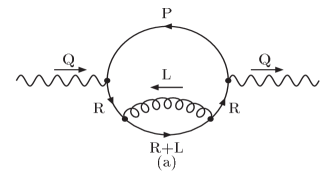
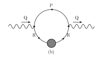
FIG. 1.: Diagrams contributing to the photon self energy for the Compton and annihilation processes when intermediate quark momentum is (a) hard (b) soft

Similarly, the photon production from bremsstrahlung and annihilation with scattering (AWS) processes can be obtained from the two loop effective diagrams as shown in Figure 2 (notations are same as given in [20, 21]).

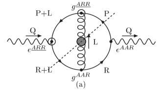
FIG. 2.: (a) Vertex and (b) Self diagram for two loop self energy in the effective theory

In section III, we estimate the above self energy (at effective two loop level) more explicitly for an unsaturated plasma as defined above.

III Photon production at two loop level

In the two loop level of effective theory the Feynmann diagrams need to be considered are shown in Figure 2. The imaginary part of the photon self energy can be expressed as a sum over the possible cuts through the effective two loop diagrams. The physical processes bremsstrahlung and quark anti-quark annihilation are obtained by cutting through the effective gluon propagator. To obtain the contribution of bremsstrahlung and AWS, the same order of magnitude as of contribution from Compton and annihilation processes, the quark momentum circulating in the loop should be hard. As a result, all the vertices and propagators can be used as bare one except for the gluon propagator since the gluon can be soft. Recall that only Landau Damping part ($L^{2}<0$) gives bremsstrahlung and AWS, whereas the $L^{2}>0$ part gives Compton and annihilation process which has been already included in the effective one loop level calculations for hard gluon exchange. However, due to phase space restriction, the Landau damping is the dominant mechanism if $L$ is soft [20].

Figure 2 shows the relevant cuts and circling required to evaluate the self energy using thermal cutting valid for RA formalism [36, 37, 43]. In the following, we extend the formalism of Aurenche et al. [20, 21] to the chemically non-equilibrated situation. An important aspect in the RA formalism is the redefined vertices which contain the distribution functions. We have derived them in appendix A for a more general situation where the plasma is chemically unsaturated as well as has non zero baryo-chemical potential. However, in the present work, we consider only a baryon free chemically unsaturated plasma. The vertex functions corresponding to Figure 2(a) are given by

$$e^{AAR}(R,-P,-Q)=e[n_{{}_{F}}(r_{0})-n_{{}_{F}}(p_{0})]$$ (6)

$$g^{AAR}(R+L,-L,-R)=g[n_{{}_{B}}(l_{0})+n_{{}_{F}}(r_{0}+l_{0})]$$ (7)

$$e^{\underline{ARR}}(Q,P+L,-R-L)=-e^{ARR}(Q,P+L,-R-L)$$ (8)

$$~{}~{}~{}~{}~{}~{}~{}~{}~{}~{}~{}~{}~{}~{}~{}~{}~{}~{}~{}~{}~{}~{}~{}~{}~{}~{}~{}~{}~{}~{}~{}~{}~{}=-e$$ (9)

$$g^{\underline{ARR}}(-P-L,P,L)=-g^{ARR}(-P-L,P,L)$$ (10)

$$~{}~{}~{}~{}~{}~{}~{}~{}~{}~{}~{}~{}~{}~{}~{}~{}~{}~{}~{}~{}~{}~{}~{}~{}~{}~{}~{}~{}~{}~{}~{}~{}~{}=-g$$ (11)

The above vertex functions are in the same form as the equilibrated case except the distribution functions should contain appropriate chemical potential. In the above example, the chemical potentials associated with $R$ and $P$ lines are $\mu_{q}$ where as it vanishes for $Q$ and $L$ lines. Therefore, using the above definitions, the vertex (Figure 2(a)) and self (Figure 2(b)) diagrams of the imaginary part of the photon self energy can be expressed as

$${\rm Im}\,\Pi^{{}^{RA}}{}_{\mu}{}^{\mu}(E,{\vec{q}})_{|_{\rm vertex}}=-{\rm Im}\,\Pi^{{}^{AR}}{}_{\mu}{}^{\mu}(E,{\vec{q}})_{|_{\rm vertex}}$$ (12)

$$={{NC_{{}_{F}}}\over 2}\int{{d^{4}P}\over{(2\pi)^{4}}}\int{{d^{4}L}\over{(2\pi)^{4}}}$$ (13)

$$\times\;e^{{}^{\underline{ARR}}}(Q,P+L,-R-L)g^{{}^{\underline{ARR}}}(-P-L,P,L)$$ (14)

$$\times\;g^{{}^{{AAR}}}(R+L,-L,-R)e^{{}^{{AAR}}}(R,-P,-Q)$$ (15)

$$\times\;{\rm Tr}\left[\gamma^{\mu}{\cal S}^{{}^{\underline{AR}}}(P+L)\gamma^{\rho}{\cal S}^{{}^{A\underline{R}}}(P)\gamma_{\mu}{\cal S}^{{}^{RA}}(R)\gamma^{\sigma}{\cal S}^{{}^{\underline{R}A}}(R+L)\right]$$ (16)

$$\times D^{{}^{A\underline{R}}}_{\rho\sigma}(L)$$ (17)

and

$$\!\!\!{\rm Im}\,\Pi^{{}^{RA}}{}_{\mu}{}^{\mu}(E,{\vec{q}})_{|_{\rm self}}=-{\rm Im}\,\Pi^{{}^{AR}}{}_{\mu}{}^{\mu}(E,{\vec{q}})_{|_{\rm self}}$$ (18)

$$={{NC_{{}_{F}}}\over 2}\int{{d^{4}P}\over{(2\pi)^{4}}}\int{{d^{4}L}\over{(2\pi)^{4}}}$$ (19)

$$\times\;e^{{}^{\underline{ARR}}}(Q,P,-R)g^{{}^{\underline{ARR}}}(R,L,-R-L)$$ (20)

$$\times\;g^{{}^{{AAR}}}(R+L,-L,-R)e^{{}^{{AAR}}}(R,-P,-Q)$$ (21)

$$\times\;{\rm Tr}\,\left[\gamma^{\mu}{\cal S}^{{}^{A\underline{R}}}(P)\gamma_{\mu}{\cal S}^{{}^{{RA}}}(R)\gamma^{\rho}\right.\left.{\cal S}^{{}^{\underline{R}A}}(R+L)\gamma^{\sigma}{\cal S}^{{}^{\underline{RA}}}(R)\right]$$ (22)

$$\times D^{{}^{A\underline{R}}}_{\rho\sigma}(L)\;.$$ (23)

According to the cutting rule valid for RA formalism [43], the fermion cut propagators are given by

$${\cal S}^{{}^{RA}}(P)\equiv{\cal S}^{{}^{A}}(P)$$ (24)

$${\cal S}^{{}^{\underline{AR}}}(P)\equiv-{\cal S}^{{}^{A}}(P)$$ (25)

$${\cal S}^{{}^{A\underline{R}}}(P)\equiv{\cal S}^{{}^{R}}(P)-{\cal S}^{{}^{A}}(P)$$ (26)

$${\cal S}^{{}^{\underline{R}A}}(P)\equiv{\cal S}^{{}^{A}}(P)-{\cal S}^{{}^{R}}(P).$$ (27)

We denote the fermion propagator:

$${\cal S}^{{}^{R,A}}(P)\equiv{\overline{P\!\!\!/}}S^{{}^{R,A}}(P){\ \rm with\ }{\overline{P}}\equiv(p_{o},\sqrt{p^{2}+M^{2}_{\infty}}\,\hat{p})$$ (28)

$$S^{{}^{R,A}}(P)\equiv{i\over{{\overline{P}}^{2}\pm ip_{o}\varepsilon}}={i\over{P^{2}-M^{2}_{\infty}\pm ip_{o}\varepsilon}}\;.$$ (29)

Similarly, boson cut propagator

$$D_{\rho\sigma}^{{}^{A\underline{R}}}(L)\equiv D_{\rho\sigma}^{{}^{R}}(L)-D_{\rho\sigma}^{{}^{A}}(L)\;.$$ (30)

The effective gluon propagator in a linear covariant gauge is given by

$$-D_{\rho\sigma}^{{}^{R,A}}(L)\equiv P^{{}^{T}}_{\rho\sigma}(L)\Delta^{{}^{R,A}}_{{}_{T}}(L)+P^{{}^{L}}_{\rho\sigma}(L)\Delta^{{}^{R,A}}_{{}_{L}}(L)$$ (31)

$$~{}~{}~{}~{}~{}~{}~{}~{}~{}~{}~{}~{}~{}~{}~{}~{}~{}~{}+\xi L_{\rho}L_{\sigma}/L^{2}$$ (32)

$$\Delta^{{}^{R,A}}_{{}_{T,L}}(L)\equiv\left.{i\over{L^{2}-\Pi_{{}_{T,L}}(L)}}\right|_{{}_{R,A}}\;.$$ (33)

Here $P^{{}^{T,L}}_{\rho\sigma}$ are the usual transverse and longitudinal projectors in linear covariant gauges [21, 44, 45] and

$$\Pi_{{}_{T}}(L)\equiv 3m_{\rm g}^{2}\left[{{x^{2}}\over 2}+{{x(1-x^{2})}\over{4}}\ln\left({{x+1}\over{x-1}}\right)\right]$$ (34)

$$\Pi_{{}_{L}}(L)\equiv 3m_{\rm g}^{2}(1-x^{2})\left[1-{{x}\over{2}}\ln\left({{x+1}\over{x-1}}\right)\right]\;,$$ (35)

where, $x=l_{0}/l$.

Using the expression of the vertices in Eq.(11) and the cut propagators, the vertex diagram of photon self energy can be simplified as

$${\rm Im}\,\Pi^{{}^{RA}}{}_{\mu}{}^{\mu}(E,{\vec{q}})_{|_{\rm vertex}}$$ (36)

$$=-{{NC_{{}_{F}}}\over 2}e^{2}g^{2}\int{{d^{4}P}\over{(2\pi)^{4}}}\int{{d^{4}L}\over{(2\pi)^{4}}}\left[\Delta^{{}^{R}}_{{}_{T,L}}(L)-\Delta^{{}^{A}}_{{}_{T,L}}(L)\right]$$ (37)

$$\times\;\left[S^{{}^{R}}(P)-S^{{}^{A}}(P)\right]\left[S^{{}^{R}}(R+L)-S^{{}^{A}}(R+L)\right]$$ (38)

$$\times\;\left(n_{{}_{F}}(r_{o})-n_{{}_{F}}(p_{o})\right)\left(n_{{}_{B}}(l_{o})+n_{{}_{F}}(r_{o}+l_{o})\right)$$ (39)

$$\times\;S(R)S(P+L)P_{\rho\sigma}^{{}^{T,L}}(L)\;{\rm Trace}^{\rho\sigma}{}_{|_{\rm vertex}}\;.$$ (40)

Similarly, the photon self energy for the self diagram can be expressed as in Ref. [21] with appropriate distribution functions

$$\!\!\!{\rm Im}\,\Pi^{{}^{RA}}{}_{\mu}{}^{\mu}(E,{\vec{q}})_{|_{\rm self}}$$ (41)

$$=-{{NC_{{}_{F}}}\over 2}e^{2}g^{2}\int{{d^{4}P}\over{(2\pi)^{4}}}\int{{d^{4}L}\over{(2\pi)^{4}}}\left[\Delta^{{}^{R}}_{{}_{T,L}}(L)-\Delta^{{}^{A}}_{{}_{T,L}}(L)\right]$$ (42)

$$\times\;\left[S^{{}^{R}}(P)-S^{{}^{A}}(P)\right]\left[S^{{}^{R}}(R+L)-S^{{}^{A}}(R+L)\right]$$ (43)

$$\times\;\left(S(R)\right)^{2}\left(n_{{}_{F}}(r_{o})-n_{{}_{F}}(p_{o})\right)\left(n_{{}_{B}}(l_{o})+n_{{}_{F}}(r_{o}+l_{o})\right)$$ (44)

$$\times P_{\rho\sigma}^{{}^{T,L}}(L)\;{\rm Trace}^{\rho\sigma}{}_{|_{\rm self}}\;$$ (45)

where $e$ is the electric charge of the quark which depends on its flavor. The trace in Eq. (40) and Eq.(45) are given by,

$${\rm Trace}^{\rho\sigma}{}_{|_{\rm vertex}} = {\rm Tr}[\gamma^{\mu}{({P\!\!\!/}+{L\!\!\!/})}\gamma^{\rho}({P\!\!\!/})\gamma_{\mu}({R\!\!\!/})\gamma^{\sigma}({R\!\!\!/}+{L\!\!\!/})]$$ (46)

$${\rm Trace}^{\rho\sigma}{}_{|_{\rm self}} = {\rm Tr}[\gamma^{\mu}{P\!\!\!/}\gamma_{\mu}({R\!\!\!/})\gamma^{\rho}({R\!\!\!/}+{L\!\!\!/})\gamma^{\sigma}{R\!\!\!/}]\;.$$ (47)

The factor $S(R)$, $S(P+L)$ without any $R$ and $A$ superscript denotes the principal part of the propagator i.e.,

$$S(R) = \frac{1}{(R^{2}-M_{\infty}^{2})}$$ (48)

$$S(P+L) = \frac{1}{((P+L)^{2}-M_{\infty}^{2})}\;.$$ (49)

The difference between the retarded and the advanced gluon propagators, in both the vertex (Eq. 40) and self (Eq. 45) part of the photon self-energy is known as spectral function given by

$$\rho_{{}_{T,L}}(L)=\Delta^{{}^{R}}_{{}_{T,L}}(L)-\Delta^{{}^{A}}_{{}_{T,L}}(L)\;.$$ (50)

The properties of these spectral functions depend upon the analytic structure of the gluon propagator. For $L^{2}<0$ (i.e. $|x|<1$) region, in which we are interested about, the self-energies $\Pi_{{}_{T,L}}$ acquire an imaginary part due to the logarithm and the corresponding expression of the spectral functions are given by,

$$\rho_{{}_{T,L}}(L)\equiv\frac{\left.{-2{\rm Im}\Pi_{{}_{T,L}}(L)}\right|_{{}_{R}}}{(L^{2}-{\rm Re}\Pi_{{}_{T,L}}(L))^{2}-(\left.{{\rm Im}\Pi_{{}_{T,L}}(L)}\right|_{{}_{R}})^{2}}\;.$$ (51)

Here the imaginary part of retarded self energies are

$$\left.{{\rm Im}\Pi_{{}_{T}}(L)}\right|_{{}_{R}}=\frac{3\pi m_{g}^{2}}{4}x(1-x^{2})$$ (52)

$$\left.{{\rm Im}\Pi_{{}_{L}}(L)}\right|_{{}_{R}}=-2\left.{{\rm Im}\Pi_{{}_{T}}(L)}\right|_{{}_{R}}\;.$$ (53)

Adding the contributions from these two diagrams and plugging into the expression (Eq.(5)), the photon production from the effective two loop level can be evaluated. It should be noticed that the expression for the self energy is same as used in [21], except for the non-equilibrium distribution functions $n_{{}_{F}}$ and thermal masses which contain chemical potentials. Like in one loop case, here also we ignore the pinch contribution and assume that the effective quark and gluon propagators are still given by their equilibrium counter part with use of asymptotic thermal quark mass $M_{\infty}^{2}=2m_{q}^{2}$ defined by

$$m_{q}^{2}=\frac{g^{2}}{3\pi^{2}}\int p~{}dp~{}[2n_{g}+(n_{q}+n_{\bar{q}})]$$ (54)

which can be shown to be $(\lambda_{g}+\frac{\lambda_{q}}{2})g^{2}T^{2}/9$ for factorized distributions. The thermal gluon mass $m_{\rm g}^{2}$ appropriate for non-equilibrium plasma [44, 46] is given by

$$m_{\rm g}^{2}=\frac{g^{2}}{3\pi^{2}}\int pdp[6n_{g}+N_{f}(n_{q}+n_{\bar{q}})]\;.$$ (55)

For a factorised distribution the $m_{g}^{2}$ can be written as $(3\lambda_{g}+\frac{N_{f}}{2}\lambda_{q})g^{2}T^{2}/9$. The kinematic conditions restrict the phase space for the physical process into three regions as shown in Figure 3.

FIG. 3.: Physical processes appear by cutting the two loop diagram of Figure 2 for $L^{2}<0$ (a) Region I: (b) Region II (c) Region III

$\displaystyle\begin{array}[!h]{cc}\mbox{Region I}&p_{0}<0~{}~{}\mbox{ and}~{}~{}r_{0}+l_{0}<0\\ \mbox{Region II}&p_{0}<0~{}~{}\mbox{ and}~{}~{}r_{0}+l_{0}>0\\ \mbox{Region III}&p_{0}>0~{}~{}\mbox{ and}~{}~{}r_{0}+l_{0}>0\\ \end{array}$

Region I and III corresponds to bremsstrahlung from anti-quark and quark respectively. The region II corresponds to AWS processes. The physical processes with the lower line in the Fig. 3 replaced with quark, anti-quark have also been included. It may be mentioned here that region I and region III will give same contribution as long as quark and anti-quark distribution functions are same (i.e. for a baryon free plasma). We will study the contribution from region III and multiply it by a factor 2 to get the total bremsstrahlung photon yield. Similarly, we will discuss about the region II for AWS process.

A Bremsstrahlung

The two points which need to be addressed here are the collinear limit and the enhancement due to collinear singularity. It is important to notice that due to the factors $[(R^{2}-M_{\infty}^{2})((P+L)^{2}-M_{\infty}^{2})]^{-1}$ which appear in the integral Eq. (40) is responsible for the collinear divergence. Although we will carry out the complete integration, even at the qualitative level, we can understand the nature of the divergence from the integral of the type

$$I\equiv\int_{0}^{2}\frac{du}{(R^{2}-M_{\infty}^{2})}\int_{0}^{2\pi}\frac{d\phi}{(P+L)^{2}-M_{\infty}^{2}}$$ (56)

where $\theta~{}(u=1-cos\theta)$ is the angle between $\vec{p}$ and $\vec{q}$ and $\phi$ is the azimuthal angle between $\vec{q}$ and $\vec{l}$ when projected on a plane orthogonal to $\vec{r}$. For hard photon production, the following approximations can be used

$$R^{2}-M_{\infty}^{2} \approx 2pq(u+a);~{}~{}a=\frac{M_{\infty}^{2}}{2p^{2}}$$ (57)

$$\int\frac{d\phi}{(P+L)^{2}-M_{\infty}^{2}} \approx \frac{2\pi(p+q)}{2qp^{2}(u+b)};~{}b=\frac{M_{\infty}^{2}}{2p^{2}}+\frac{L^{2}}{2p^{2}}$$ (58)

In the above, $(b-a)\sim L^{2}/p^{2}$ gives a measure of the distance between the two poles. Since the two poles are very near by (for soft gluon exchange), the above integral is of the order

$$I\sim\frac{p+q}{p(p^{2}q^{2})a}$$ (59)

for $a>L^{2}/p^{2}$ or $M_{\infty}^{2}>L^{2}$. Note that this enhancement factor which is associated with the smallness of the angle of emission is same irrespective of whether the emitted photon is soft or hard. As a consequence, the integral is enhanced by a factor of order $p^{2}/M_{\infty}^{2}\sim 1/(g^{2}\lambda_{g})$ if the plasma is strongly gluon dominated i.e. $\lambda_{q}<\lambda_{g}\ll 1$. The above enhancement is larger by a factor of $\lambda_{g}^{-1}$ as compared to the equilibrated case. Although the above argument is qualitative, it remains valid even after all the integrations are carried out (see Figure 4 in section IV). Now, proceeding as before [21] under collinear approximation, the expression for the imaginary part of self energy can be written as

$${\rm Im}\,\Pi^{{}^{AR}}{}_{\mu}{}^{\mu}{}(E,{\vec{q}})$$ (63)

$$\approx(-1)_{T}\frac{NC_{F}}{4\pi^{4}}e^{2}g^{2}\frac{1}{E^{2}}\int_{p^{\ast}}^{\infty}[n_{{}_{F}}(p)-n_{{}_{F}}(p+E)]$$

$$\times(p^{2}+(p+E)^{2})~{}dp\int_{0}^{l^{\ast}}l^{4}~{}dl\int_{-1}^{1}dx\int_{0}^{1}du^{\prime}~{}n_{{}_{B}}(lx)$$

$$\times\rho_{T,L}(l,lx)(1-x^{2})^{2}(1-u^{\prime})^{-1/2}(4M_{\infty}^{2}+l^{2}(1-x^{2})u^{\prime})^{-1}$$

where $u^{\prime}\equiv-8r^{2}u/L^{2}$ and the symbol $(-1)_{T}$ denotes an extra minus sign in the transverse contribution. Here we have introduced some cut-offs $p^{\ast}$ and $l^{*}$ at a scale intermediate between $gT$ and $T$, where we assume $r$ to be hard and $l$ to be negligible compared to $T$. We have ignored the factor $n_{{}_{F}}(r_{0}+l_{0})$ since it is much smaller compared to the Bose distribution $n_{{}_{B}}(l_{0})$ (where $l_{0}=lx$) particularly for unsaturated QGP. As a result, the integral over $p$ becomes independent of integrals over $L$. The Bose-distribution is also approximated to $n_{{}_{B}}(lx)\sim\frac{T}{lx}$. This assumption considerably simplifies the numerical evaluation of the self energy which can be expressed in terms of the dimensionless constants $J_{T}$ and $J_{L}$,

$$J_{T,L} = \int_{0}^{1}\frac{dx}{x}{\tilde{I}}_{T,L}(x)$$ (66)

$$\times\int_{0}^{w^{*}}dw\frac{\sqrt{\frac{w}{w+4}}\tanh^{-1}\sqrt{\frac{w}{w+4}}}{(w+{\tilde{R}}_{T,L}(x))^{2}+({\tilde{I}}_{T,L}(x))^{2}}$$

where

$$w\equiv\frac{-L^{2}}{M_{\infty}^{2}},~{}~{}~{}~{}~{}~{}~{}~{}{\tilde{I}}_{T,L}(x)\equiv\frac{{\rm Im}\Pi_{T,L}(x)}{M_{\infty}^{2}},$$ (67)

$${\tilde{R}}_{T,L}(x)\equiv\frac{{\rm Re}\Pi_{T,L}(x)}{M_{\infty}^{2}}.$$ (68)

Note that we do not assign any chemical potential to the gluon line $L$ leading to the approximation $\frac{T}{lx}$ rather than $\lambda_{g}\frac{T}{lx}$ (see subsection $D$ for more discussion). The functions $J_{T},~{}J_{L}$ depend on the thermal mass ratio $m_{\rm g}^{2}/M_{\infty}^{2}$ and $l^{\ast}/M_{\infty}$. Notice that the above expressions for $J_{T}$ and $J_{L}$ are same as in Ref.[21] except that the thermal masses now depend on the chemical potentials or fugacities. It has been shown in [20, 21] that for equilibrated plasma, taking $w^{\ast}\rightarrow\infty$ introduces a negligible contribution to the integration of $J_{T,L}$. This argument is also valid for chemically non-equilibrated plasma since the value of $w^{\ast}$ increases with decreasing fugacity. Thus extrapolating the upper limit of the integration $w^{\ast}$ to $\infty$ introduces smaller error as compared to the equilibrated plasma and can be neglected. Finally, the imaginary part of the self energy can be written as

$${\rm Im}\,\Pi^{{}^{AR}}{}_{\mu}{}^{\mu}{}(E,{\vec{q}})$$ (69)

$$\approx \frac{NC_{F}}{\pi^{4}}e^{2}g^{2}(J_{T}-J_{L})\frac{T}{E^{2}}$$ (71)

$$\times\int_{0}^{\infty}[n_{{}_{F}}(p)-n_{{}_{F}}(p+E)](p^{2}+(p+E)^{2})~{}dp$$

The total photon production rate for bremsstrahlung process can be evaluated as

$$\left.2E\frac{dR}{d^{3}q}\right|_{brem}\approx 4\frac{NC_{F}\alpha\alpha_{s}}{\pi^{5}}\left(\sum_{f}e_{f}^{2}\right)~{}\frac{T}{E^{2}}(J_{T}-J_{L})$$ (72)

$$\times n_{{}_{B}}(E)~{}\int_{0}^{\infty}dp~{}(p^{2}+(p+E)^{2})[n_{{}_{F}}(p)-n_{{}_{F}}(p+E)]$$ (73)

where $e_{f}$ is the electric charge of the quark flavor $f$ in units of electron charge and $n_{{}_{B}}(E)=[\exp(E/T)-1]^{-1}$ is the prefactor independent of any chemical potential for the bremsstrahlung process. The $J_{T}$ and $J_{L}$ integrals depend only on the thermal mass ratio $m_{g}^{2}/M_{\infty}^{2}$ and are insensitive to the chemical potential or fugacity. Since the prefactor $n_{B}(E)$ is independent of $\mu$ for bremsstrahlung, the chemical unsaturation effect enters only through the quark distribution functions $n_{F}(p)$ in the $p$ integral. Therefore, for factorized distribution functions, the bremsstrahlung contribution from non-equilibrated plasma is suppressed by a factor of $\lambda_{q}$ as compared to the equilibrium case.

B Annihilation with scattering

In case of $q{\bar{q}}$ annihilation with scattering (AWS), one should consider the region II where $p_{0}<0$. The procedure to estimate AWS rate is nearly identical to that of bremsstrahlung except for the exchanges $u\rightarrow v$ and $p\rightarrow-p$ where $v=1+\cos\theta$. In this case also the enhancement mechanism remains same as before. Finally, with the replacement of $p$ by $-p$, the $p$ integral in Eq.( LABEL:self) can be written as

$$\left.2E\frac{dR}{d^{3}q}\right|_{AWS}\approx 2\frac{NC_{F}\alpha\alpha_{s}}{\pi^{5}}\left(\sum_{f}e_{f}^{2}\right)~{}\frac{T}{E^{2}}(J_{T}-J_{L})$$ (74)

$$\times n_{{}_{B}}(E)~{}\int_{0}^{\infty}dp(p^{2}+(E-p)^{2})[n_{{}_{F}}(-p)-n_{{}_{F}}(E-p)]$$ (75)

where $n_{{}_{F}}(-p)=1-n_{{}_{F}}(p)$. For equilibrated plasma, the contribution from $[n_{{}_{F}}(-p)-n_{{}_{F}}(E-p)]$ is assumed $\sim 1$. This approximation is also valid in case of non-equilibrated plasma since the distribution functions are smaller by a factor of $\lambda_{q}$. The unsaturation effect appears through the prefactor $n_{{}_{B}}(E)$ which goes as $[\exp(E/T)-1]^{-1}\lambda_{q}^{2}$ under factorized approximation (see the discussions in appendix A). Therefore, the AWS photon production is suppressed by a factor of $\lambda_{q}^{2}$ as compared to its equilibrium counterpart.

Finally, we would like to end this sub-section with the remark that both bremsstrahlung and AWS photon productions for non-equilibrated plasma are suppressed by a factor of $\lambda_{q}$ and $\lambda_{q}^{2}$ respectively due to unsaturated quark and anti-quark distribution functions. The suppression due to unsaturated gluon distribution function seems to get compensated by the additional enhancement caused by collinear singularity.

C Factorisation and Kinetic theory

In this section, we establish a connection between the field theoretical formalism as given in previous sub-section and relativistic kinetic theory which can also be used to estimate the photon production rate under semiclassical approximation [20, 47]. Consider the case of photon production due to bremsstrahlung. In the kinetic theory approach, the photon production rate can be evaluated by integrating the amplitude squared of the process over the phase space of unobserved particles and given by

$$\frac{dR}{d^{3}q}=\frac{1}{(2\pi)^{3}~{}2E}\int\frac{d^{4}p}{(2\pi)^{4}}\int\frac{d^{4}K}{(2\pi)^{4}}\int\frac{d^{4}L}{(2\pi)^{4}}$$ (76)

$$\times\left|\raisebox{-25.6073pt}{\begin{picture}(130.0,15.0)(0.0,0.0){ \mbox{\psfig{}} }\end{picture}}\right|^{2}$$ (77)

$$\times 2\pi\delta(P^{2}-M_{\infty}^{2})~{}2\pi\delta((R+L)^{2}-M_{\infty}^{2})$$ (78)

$$\times 2\pi\delta(K^{2}-M_{\infty}^{2})~{}2\pi\delta((K+L)^{2}-M_{\infty}^{2})$$ (79)

$$\times n_{{}_{F}}(r_{0}+l_{0})~{}n_{{}_{F}}(k_{0})~{}[1-n_{{}_{F}}(p_{0})]~{}[1-n_{{}_{F}}(k_{0}+l_{0})]$$ (80)

(81)

Here we have only considered the amplitude for the bremsstrahlung process where quark has been scattered from another quark. In order to get total photon production rate from bremsstrahlung, the processes involving quark scattered from a gluon or an anti-quark also have to be considered.

In order to establish a connection to field theory, we now look for various statistical factors that appear in Eq.(81). Let us consider the product of all the distribution functions that appear in the calculation of self energy [see Eq.(5) and Eq.(40)]

$$n_{{}_{B}}(q_{0})[n_{{}_{B}}(l_{0})+n_{{}_{F}}(r_{0}+l_{0})]$$ (84)

$$\times[n_{{}_{F}}(r_{0})-n_{{}_{F}}(p_{0})][n_{{}_{F}}(k_{0}+l_{0})-n_{{}_{F}}(k_{0})]$$

$$=n_{{}_{F}}(r_{0}+l_{0})[1-n_{{}_{F}}(p_{0})]n_{{}_{F}}(k_{0})[1-n_{{}_{F}}(k_{0}+l_{0})]$$

The pre-factor $n_{{}_{B}}(q_{0})$ ($q_{0}=E$) comes from Eq.(5) while the second and third factors come from the vertex functions $g^{AAR}$ and $e^{AAR}$. Although not explicit in Eq.(40), the last factor appears due to the hard thermal quark loop contribution to the gluon self energy [20]. In the last factor, $n_{{}_{F}}$ will be replaced by $n_{{}_{B}}$ when the quark scattering from gluon is considered. For the above identity to be valid, the distribution functions should be defined properly with appropriate chemical potentials. For example, in case of bremsstrahlung, the chemical potential for $Q$ and $L$ lines are zero where as chemical potentials for $R+L$, $R$ and $P$ lines are $\mu_{q}$. Similarly, the chemical potentials for $K$ and $K+L$ lines are $\mu_{q}$ for quark loop and $\mu_{g}$ for gluon loop respectively (see appendix A for detail). The baryo-chemical potential is zero since we restrict only to the case of a baryon free plasma. Due to the validity of the above factorisation, similar to the case of an equilibrated plasma [20, 21], we can show the equivalence between two approaches based on field theory and kinetic theory. Similar arguments also apply for the case of annihilation with scattering due to the following identity (given only for quark quark scattering)

$$n_{{}_{B}}(q_{0})[n_{{}_{B}}(l_{0})+n_{{}_{F}}(r_{0}+l_{0})]$$ (87)

$$\times[n_{{}_{F}}(r_{0})-n_{{}_{F}}(-p_{0})][n_{{}_{F}}(k_{0}+l_{0})-n_{{}_{F}}(k_{0})]$$

$$=n_{{}_{F}}(r_{0}+l_{0})n_{{}_{F}}(p_{0})n_{{}_{B}}(k_{0})[1-n_{{}_{F}}(k_{0}+l_{0})].$$

The above identity is quite similar to Eq.(84) except that the chemical potential associated with the pre-factor $n_{B}(q_{0})$ is $2\mu_{q}$.

Recently, Mustafa et al. [35] have calculated the photon production from a non-equilibrated plasma based on the above kinetic theory approach. Assuming a factorized form of parton distribution functions i.e. $n_{i}=\lambda_{i}n_{i}^{eq}$ where $n_{i}^{eq}$ is the distribution function at equilibrium and combining the contributions from quark and gluon scattering with appropriate spin, colour and flavour statistics, the rate for the bremsstrahlung production can be written as [see Eq.(81)].

$$\frac{dR}{d^{3}q} = (\frac{A}{A+B}\lambda_{g}\lambda_{q}+\frac{B}{A+B}\lambda_{q}^{2})\times{\cal R}$$ (88)

$$= \lambda_{q}(\frac{2}{5}\lambda_{g}+\frac{3}{5}\lambda_{q})\times{\cal R}$$ (89)

where $\cal R$ is the equilibrium contribution to photon production, ${\cal R}=(A+B)\cal I$ with $\cal I$ given by Eq.(81) to be evaluated under classical approximation. The degeneracy factors $A$ and $B$ are given by

$$A = \frac{4}{9}\times 2\times 2_{f}\times 2_{s}\times 3_{c}=\frac{32}{3}~{}~{}~{};$$ (90)

$$B = 2_{s}\times 8_{c}=16.$$ (91)

The factor $4/9$ in the expression for $A$ appears due to the assumption $|{\cal M}|^{2}_{q\leftrightarrow q}=4/9|{\cal M}|^{2}_{q\leftrightarrow g}$ where $|{\cal M}|^{2}_{q\leftrightarrow q}$ and $|{\cal M}|^{2}_{q\leftrightarrow g}$ are the square of the matrix element for quark-quark scattering and quark-gluon scattering respectively [47]. Recall that it is possible to combine the quark and gluon contribution in a form given by Eq.(89) only if $n_{{}_{F}}\approx n_{{}_{B}}$ and quantum statistics are ignored in Eq.(81) which is true under classical approximation. In this context, the factorisation in Eq.(89) is only approximate. This has been the basis of the result used in Ref. [35], although they subsequently use correct equilibrated value for $\cal R$ obtained from the imaginary part of the photon self energy. Note that in Ref. [35], instead of $2/5$ and $3/5$ as in Eq.(89), these factors are found to be $3/7$ and $4/7$ respectively. Apart from this minor discrepancy, the use of equilibrium value for $\cal R$ is incorrect for the following reason even though Eq.(89) is approximately correct as mentioned before. The factor $\cal R$ contains the square of the matrix elements involving the product of the terms $(R^{2}-M_{\infty}^{2})$ and $(P+L)^{2}-M_{\infty}^{2}$ in the denominator. Due to the presence of two very near by poles, the matrix element will be enhancement by an factor of $\sim p^{2}/M_{\infty}^{2}$ while the enhancement would have been logarithmic if only one of the terms appear in the denominator. Therefore, there is an additional enhancement $\sim(2~{}\lambda_{g}+\lambda_{q})/3$ if the plasma is unsaturated. This additional enhancement will be compensated to a large extent by the suppression factor given in Eq.(89) above particularly when the plasma is gluon dominated. In addition to taking out the fugacity factors from the distribution functions appearing in Eq.(81), the square of the amplitude should also be calculated properly for a non-equilibrated plasma. Although a detailed calculation needs to be carried out, naively, $\cal R$ should differ from the equilibrium value by a factor of $\sim\lambda_{g}^{-1}$ when $\lambda_{q}\ll\lambda_{g}\ll 1$. A comparison with Eq.(89) suggests that the photon production rate for bremsstrahlung should have strong dependence on $\lambda_{q}$ which (within above approximations) is consistent with the results obtained in section III. Based on the similar arguments, it can be shown that the AWS photon production will depend only on $\lambda_{q}^{2}$.

D Suppression and Enhancement mechanism

Let us now summarize why the suppression and partial compensation occur when the plasma is unsaturated. First, it may be easier to understand from the kinetic theory arguments. For example, consider the case of bremsstrahlung due to quark-quark scattering [see Eq.(81) and Eq.(84)]. The suppression is due to the unsaturated distribution functions $n_{{}_{F}}(r_{0}+l_{0})$ and $n_{{}_{F}}(k_{0})$ that appear in the initial states. Similar suppression occurs in case of quark-gluon scattering except $n_{{}_{F}}(k_{0})$ has to be replaced by $n_{{}_{B}}(k_{0})$. The above suppression is partially compensated by an additional enhancement factor that arise due to the mass effect in the matrix element. It may be noted here that the gluon distribution that appears in the initial and final states comes through cutting the effective gluon propagator. In the field theoretical description, $n_{{}_{B}}(k_{0})$ does not appear explicitly, but contained in the effective gluon propagator through the thermal gluon mass $m_{g}^{2}$. Further, notice that the soft gluon associated with $n_{{}_{B}}(l_{0})$ and responsible for scattering has no role in the above suppression.

The same thing happens in the field theoretical description as well. Since $R+L$ and $R$ correspond to the same quark in the initial and final states of scattering, we assign same fugacity to both $R+L$ and $R$ lines. This argument is also consistent with the kinetic theory for the fact that any of the physical processes do not change the quark contents in the final states. Therefore, it is reasonable to assume the same chemical potential both for the initial and final quark lines i.e. to both $R+L$ and $R$ lines. From the conservation of potential, it follows that $L$ line should have zero chemical potential or unit fugacity. Therefore, $n_{{}_{B}}(l_{0})$ still follows the Bose distribution. Then, how do we understand the suppression due to gluon fugacity which gets compensated by the additional linear enhancement ? Let us consider Eq.(66) again. In case of equilibrated plasma, it is shown [20] that Eq.(66) depends only on the ratio $m_{g}^{2}/M_{\infty}^{2}$. The integrals $J_{T}$ and $J_{L}$ diverge if the thermal quark mass $M_{\infty}$ is switched off. Therefore, the above singularity is regularized by this thermal quark mass. In case of non-equilibrated plasma, $M_{\infty}^{2}$ decreases giving enhancement in $J_{T}$ and $J_{L}$. However, this enhancement is compensated by a simultaneous decrease in $m_{g}^{2}$. To be more explicit, $M_{\infty}^{2}$ differs from the equilibrium value $(g^{2}T^{2}/6)$ by a factor of $(2\lambda_{g}+\lambda_{q})/3$. Similarly, $m_{g}^{2}$ differs from the equilibrium value $(4g^{2}T^{2}/9)$ by a factor of $(3\lambda_{g}+\lambda_{q})/4$ when $N_{f}=2$. For $\lambda_{g}=\lambda_{q}=1$, the ratio $m_{g}^{2}/M_{\infty}^{2}$ is 1.33. Under two extreme conditions, $\lambda_{q}\ll\lambda_{g}$ and $\lambda_{g}\ll\lambda_{q}$, the above ratios are 1.5 and 1.0 respectively. The corresponding changes in the $J_{T}$ and $J_{L}$ values are within $5\%$ to $10\%$ of the equilibrated values and can be ignored. Therefore, it is fair enough to say that the enhancement due to the decrease in $M_{\infty}^{2}$ gets (nearly) compensated by the corresponding decrease in $m_{g}^{2}$. In other words, for a gluon dominated plasma, the collinear enhancement and the suppression due to gluon fugacity cancels out leaving $J_{T}$ and $J_{L}$ practically unchanged. The only factor that suppresses the yield is the $p$ integral in case of bremsstrahlung that involves only the quark and anti-quark fugacities and the prefactor $n_{{}_{B}}(E)$ in case of annihilation with scattering.

E One loop results for comparison

For the completeness and also for comparison, in the following, we briefly mention our previous results for effective one loop level for the case of a non-equilibrated plasma at zero baryon density. The physical processes of photon production (annihilation $q{\bar{q}}\rightarrow g\gamma$ and Compton processes $q({\bar{q}})g\rightarrow q({\bar{q}})\gamma$) in the lowest order of perturbative expansion $({\cal O}(\alpha\alpha_{s}))$ are obtained by cutting the loop diagram as shown in Figure 1. Since the self energy is IR divergent in the soft momentum limit, a cut-off parameter $k_{c}^{2}$ is introduced to separate the soft from the hard momenta of the intermediate quark. The soft part is obtained from a resummed quark propagator and it involves a thermal quark mass which acts as an infrared cutoff. The hard part is obtained from the relativistic kinetic theory from the expression

$$2E\frac{dR^{hard}}{d^{3}q}=\frac{N}{(2\pi)^{8}}\int\frac{d^{3}p_{1}}{2E_{1}}\frac{d^{3}p_{2}}{2E_{2}}\frac{d^{3}p_{3}}{2E_{3}}~{}n_{1}(E_{1})~{}n_{2}(E_{2})$$ (92)

$$\times(1\pm n_{3}(E_{3}))\delta(p_{1}^{\mu}+~{}p_{2}^{\mu}-~{}p_{3}^{\mu}-~{}q^{\mu})\sum|{\cal M}|^{2}$$ (93)

by carrying out integration above the cut-off [13, 16, 48]. In the above, $n_{1,2,3}$ are the parton distribution functions with plus sign for annihilation and the minus sign for the two Compton processes. The total rate can be obtained by adding soft and hard contributions together. The cutoff dependence cancels out in the summation. It is also found that the total photon rate can be obtained from the hard part alone by using the lower limit of integration $k_{c}^{2}$ equal to $2m_{q}^{2}$ where the thermal quark mass $m_{q}^{2}$ is given in Eq. (54). Therefore, Eq.(93) can be used to estimate the rate of photon production using appropriate distribution functions and thermal quark mass for non-equilibrium plasma. Although the Juttner functions for parton distributions can be used, we restrict to the factorized form for convenience. However, our conclusions are independent of the above choice. Using factorized distributions and the identity,

$$n_{1}~{}n_{2}(1\pm n_{3}) = \lambda_{1}\lambda_{2}\lambda_{3}n_{1}^{eq}~{}n_{2}^{eq}~{}(1\pm n_{3}^{eq})$$ (95)

$$+\lambda_{1}\lambda_{2}(1-\lambda_{3})n_{1}^{eq}~{}n_{2}^{eq}.$$

the above equation can be broken into two parts [15, 16]. For the first part, one can use the analytic form that can be obtained using Boltzmann distribution for $n_{1}$ and $n_{2}$ [13]

$$\left(2E\frac{dR}{d^{3}q}\right)_{1}=\frac{5\alpha~{}\alpha_{s}}{9~{}\pi^{2}}~{}T^{2}~{}e^{-E/T}$$ (96)

$$\times\Biggl{[}~{}\underbrace{~{}\lambda_{q}^{2}\lambda_{g}\left\{\frac{2}{3}~{}ln\left(\frac{4~{}ET}{k_{c}^{2}}\right)-1.43\right\}}_{annihilation}$$ (97)

$$+~{}\underbrace{~{}2\lambda_{q}^{2}\lambda_{g}\left\{\frac{1}{6}ln\left(\frac{4~{}ET}{k_{c}^{2}}\right)+0.0075\right\}}_{Compton}\Biggr{]}$$ (98)

Following Ref. [15], the second part can be written as

$$\left(2E\frac{dR}{d^{3}q}\right)_{2}=\frac{10\alpha~{}\alpha_{s}}{9~{}\pi^{4}}~{}T^{2}~{}e^{-E/T}$$ (99)

$$\times\Biggl{[}\underbrace{\lambda_{q}^{2}(1-\lambda_{g})\Biggl{\{}-2-2\beta+2~{}ln\left(\frac{4~{}ET}{k_{c}^{2}}\right)\Biggr{\}}}_{annihilation}$$ (100)

$$+~{}\underbrace{\lambda_{q}\lambda_{g}(1-\lambda_{q})\Biggl{\{}1-2\beta+2~{}ln\left(\frac{4~{}ET}{k_{c}^{2}}\right)\Biggr{\}}}_{Compton}\Biggr{]}$$ (101)

where $\alpha$, $\alpha_{s}$ are electromagnetic and strong coupling constants respectively and $\beta=0.577$ is the Euler constant. In the above, the first term is the contribution from the annihilation whereas the second and third terms are due to Compton like processes. The total rate is estimated by adding Eq.(98) and Eq.(101). It may be pointed out here that Baier et al. [17] have also estimated the rate for a non-equilibrated plasma. Although the order of magnitude is same, the above expressions are different from the result given in [17] due to Boltzmann approximations for the initial states. We have also compared the above results with the exact numerical calculations using Eq.(93) and find good agreement. Therefore, we prefer to retain the above form for consistency with our previous work [16].

IV Result and discussion

In the following, we estimate numerically photon production rates for various processes. The crucial aspect of the calculation is the numerical integration of the $J_{T}$ and $J_{L}$ functions which depend sensitively only on the ratio $m_{\rm g}^{2}/M_{\infty}^{2}$.

FIG. 4.: The variation of $J_{T}$ and $J_{L}$ with $m_{\rm g}^{2}/M_{\infty}^{2}$

Figure 4 shows the plot of $J_{T}$ and $J_{L}$ over a range of mass ratios which is of interest in the present study. Although $J_{T}$ and $J_{L}$ diverge logarithmically in the limit $M_{\infty}\rightarrow 0$, it has approximately a linear dependence in the above region. In case of equilibrated plasma, the above mass ratio is about $1.33$ (for $N=3$ and $N_{f}=2$) and the corresponding $J_{T}$ and $J_{L}$ values are found to be 1.108 and -1.064 respectively [34]. Note that these values are less exactly by a factor of $4$ than the values originally reported in [20, 21] and used subsequently by many others. Since the variation of $m_{\rm g}^{2}/M_{\infty}^{2}$ with fugacity is not significant, we also use the above values for $J_{T}$ and $J_{L}$ both for equilibrated and non-equilibrated plasma.

Figure 5(a) shows the comparison between one and two loop contributions to photon self energy evaluated with the corrected values of $J_{T}$ and $J_{L}$. As in [21] bremsstrahlung dominates in the low momentum region whereas AWS dominates in the higher momentum scale. Figure 5b shows the photon production rate at a fixed temperature $T=0.57$ GeV for a chemically equilibrated plasma ($\lambda_{g}=\lambda_{q}=1.0$). The two loop contribution (bremsstrahlung + AWS) competes or even dominates over one loop photon production over a wide energy range. Further, it is noticed that the bremsstrahlung process has strong contribution to photon production below $E\sim 1$GeV and falls at a faster rate as compared to the one loop contribution particularly at higher energy. Since the $J_{T}$ and $J_{L}$ factors are same, the bremsstrahlung and AWS photon productions differ only due to different phase space factors. The $p$-integral in Eq.(73) involves the quark distribution functions $n_{{}_{F}}(p)-n_{{}_{F}}(p+E)$ whereas the $p$-integral in Eq.(75) is nearly independent of distribution functions for $0<p<E$ and has insignificant contribution for $p>E$. Therefore, the phase space suppression is stronger for bremsstrahlung as compared to the AWS process. The most significant contribution to photon production comes from the AWS process at higher photon energies. Our results obtained with the correct $J_{T}$ and $J_{L}$ values are qualitatively in agreement with the conclusions drawn from the earlier studies of Aurenche et al.

Next, we consider a chemically unsaturated plasma with two different initial conditions at RHIC bombarding energy. Figure 6(a) corresponds to the initial conditions $T=0.57$ GeV, $\lambda_{g}=0.09$ and $\lambda_{q}=0.02$ as obtained from HIJING model calculation [25] whereas Figure 6(b) is plotted with the initial conditions $T=0.67$ GeV, $\lambda_{g}=0.34$ and $\lambda_{q}=0.064$ corresponding to a typical SSPC model [35]. Note that in both cases the initial plasma is gluon dominated. A general observation is that the AWS contribution is less than the one loop contributions and the bremsstrahlung seems to be the dominant mechanism of photon production over a wide range of energy particularly when the plasma is strongly unsaturated. The above results can be understood as follows. The dominant contributions to photon production at the one loop level comes from the term which is linear in $\lambda_{q}\lambda_{g}$ [see Eq.(98) and Eq.(101)]. Also see Eq.(45) of Ref. [17]. Since the $J_{T}$ and $J_{L}$ are insensitive to fugacities, the contributions at the two loop level (say) bremsstrahlung is suppressed by a factor of $\lambda_{q}$.

FIG. 5.: (a) The photon self energy for one loop and two loop processes as a function of photon energy. (b) The rate of photon production for an equilibrated plasma ($\lambda_{g}=\lambda_{q}=1.0$) at constant temperature $T=0.57$ GeV

Similarly, the AWS process is suppressed by a factor of $\lambda_{q}^{2}$ that arises due to the prefactor although $p$-integral is nearly independent of any distribution functions. As a consequence, the AWS process is suppressed strongly as compared to the both one loop and bremsstrahlung processes. Interestingly, it is the bremsstrahlung which dominates the photon production at all energies. This is to be contrasted with the equilibrium situation where the AWS is the dominant mechanism of photon production at higher energies. Naively, from the kinetic theory arguments, it is expected that for an unsaturated plasma (gluon dominated), the bremsstrahlung and the AWS processes will be reduced by a factor of $\lambda_{q}\lambda_{g}$ and $\lambda_{q}^{2}\lambda_{g}$ respectively. However, the suppression due to $\lambda_{g}$ gets compensated by the collinear enhancement which goes up by a factor of $\lambda_{g}^{-1}$. These findings are also quite intuitive with processes initiated by one quark in the initial state being less suppressed than those initiated by two quarks. Therefore the suppression factors for the AWS, one-loop and the bremsstrahlung processes are $\lambda_{q}^{2}$, $\lambda_{q}\lambda_{g}$ and $\lambda_{q}$ respectively.

FIG. 6.: The rate of photon production at (a) $T=0.57$ GeV, $\lambda_{g}=0.09$, $\lambda_{q}=0.02$ corresponds to HIJING model and at (b) $T=0.67$ GeV, $\lambda_{g}=0.34$, $\lambda_{q}=0.064$ corresponds to SSPC model

V Conclusion

The effect of chemical potential on photon production from a quark gluon plasma has been studied. Since, the non-vanishing chemical potential characterizes an unsaturated phase space, the contributions to photon productions both at effective one and two loop levels are suppressed as compared to their equilibrium counterparts. The contributions at the effective two loop level i.e. the bremsstrahlung and annihilation with scattering (AWS) processes are suppressed by a factor of $\lambda_{q}$ and $\lambda_{q}^{2}$ respectively. Interestingly, the above suppressions are found to be independent of the gluon fugacity $\lambda_{g}$. The reduction in the photon production rate due to unsaturated gluon distribution gets compensated to the large extent by the collinear enhancement. This aspect can be understood from the kinetic theory formalism. However, there is no such enhancement for annihilation and Compton processes at the one loop level and the rate of photon production is suppressed by a factor of $\sim\lambda_{q}\lambda_{g}$. Therefore, in case of an unsaturated plasma, the AWS process is more suppressed as compared to the one loop contributions which itself is less by a factor of $\lambda_{g}$ compared to the bremsstrahlung process. This is in contrast to the equilibrium scenario where AWS dominates the photon production followed by one loop and bremsstrahlung contributions. In either case, whether the plasma is saturated or unsaturated, the two loop contributions seem to dominate over the one loop processes particularly at higher photon energies.

Further, we would like to mention here that an inherent assumption which has gone into the above formalism is the infinite lifetime of the plasma. As a consequence, the photon production rate is independent of time and depends only on the photon energy and the temperature of the plasma. The consideration of the finite life time of the plasma will lead to the time dependent production rate which may enhance the photon production further. The finite life time effect has been studied in [49] where the plasma is assumed to be both in thermal and chemical equilibrium. Although the emission rate is a non-equilibrium phenomena, the present study is quite different in the sense that the non-equilibrium here refers to a chemically unsaturated plasma that evolves with time. The basic production rate is still static, but the time dependence arises due to the hydrodynamical evolution of the plasma. Therefore, a meaningful quantity that can be compared with the experimental results is the space time integrated photon yields from a plasma undergoing chemical equilibrium. Such a study is being carried out and will be published elsewhere.

RA formalism at finite chemical potential

We generalize the RA formalism [36, 37] appropriate for an unsaturated quark gluon plasma (QGP) at finite baryon density. Since the QGP is in a thermalized state, the parton distributions can be described by the Juttner functions with non-vanishing chemical potential $\mu$. This $\mu$ can be decomposed as a sum of two components $\mu^{c}$ and $\mu^{b}$ where $\mu^{c}$ characterizes the unsaturated properties and $\mu^{b}$ is associated with the finite baryon density of the plasma.

The propagators in RA formalism are $2\times 2$ diagonal matrices, constructed from the retarded and advanced propagators of the T=0 theory while all the temperature dependence appears in the vertices. The propagators for fermions and (gauge) bosons, defined on the contour characterized by $\sigma$, can be written as,

$${\cal S}_{F}(P) = (P\!\!\!/+M)~{}~{}U^{[\eta]}(P)~{}D(P)~{}V^{[\eta]}(P)$$ (102)

$${G}_{B}^{\mu\nu}(P) = -g^{\mu\nu}~{}~{}U^{[\eta]}(P)~{}D(P)~{}V^{[\eta]}(P)$$ (103)

where $[\eta]=B(F)$ for bosonic (fermionic) propagators and $D(P)$ is the diagonal matrix

$$D(P)=\left(\begin{array}[]{cc}\Delta_{R}(P)&0\\ 0&\Delta_{A}(P)\end{array}\right)$$ (104)

with the retarded and advanced propagators given by

$$\Delta_{R,A}(P)=\frac{i}{P^{2}-M^{2}\pm i\epsilon p_{0}}$$ (105)

The matrices $U$ and $V$ are defined as

$$U^{[\eta]}(P)=e^{\beta(p_{0}-\mu)}n^{[\eta]}(p_{0})\left(\begin{array}[]{cc}b^{-1}&\eta c^{-1}e^{(\sigma p_{0}-x)}\\ b^{-1}e^{-\sigma p_{0}}&c^{-1}\end{array}\right)$$ (106)

$$V^{[\eta]}(P)=\left(\begin{array}[]{cc}b&\eta be^{(\sigma p_{0}-x)}\\ -ce^{-\sigma p_{0}}&-c\end{array}\right)$$ (107)

where $b$ and $c$ are arbitrary scalar functions of $P$, $\eta=\pm 1$ for a boson(fermion) and n${}^{[\eta]}(p_{0})$ is the usual Bose-Einstein or Fermi-Dirac distribution defined as

$$n^{[\eta]}(p_{0})=\frac{1}{e^{x}-\eta};~{}~{}~{}~{}~{}x=\beta(p_{0}-\mu)$$ (108)

$\beta$ being the inverse of temperature and $\mu$ is the chemical potential as defined above. In the RA formalism, $U$ is associated to an outgoing line while $V$ is associated to an incoming line. All the temperature dependence which is contained in $U$ and $V$ will then appear in the vertices.

The different types of vertices are calculated depending on the momentum flow. Let us consider a vertex with all lines incoming as shown in Figure A1.

FIG. A1.: (a) EM and (b)Strong vertices

The new vertex function has the form

$$-i\gamma_{\alpha\beta\rho}(P,Q,R)=-ig_{abd}V^{F}_{\alpha a}(P)~{}V^{B}_{\beta b}(Q)~{}V^{F}_{\rho d}(R)$$ (109)

The Greek indices take the value R or A and the Latin indices refer to the $1$ (particle) $2$ (ghost) of the usual formulation of the real time formalism (RTF) so that $g_{111}=\zeta$, $g_{222}=-\zeta$, where $\zeta$=$e$ or $g$ depending on the electromagnetic or strong vertex and all other couplings being zero. From the definitions above it can be shown that,

$$\gamma_{\alpha\beta\rho}(P,Q,R)=\zeta[b(P)]^{\delta_{\alpha R}}[b(Q)]^{\delta_{\beta R}}[b(R)]^{\delta_{\rho R}}$$ (110)

$$\times[-c(P)]^{\delta_{\alpha A}}[-c(Q)]^{\delta_{\beta A}}[-c(R)]^{\delta_{\rho A}}~{}e^{\sigma L_{0}}$$ (111)

$$\left[1-(-1)^{\delta_{\alpha R}+\delta_{\rho R}}~{}e^{-\beta~{}L_{0}^{\prime}}\right]$$ (112)

with $L_{0}=p_{0}\delta_{\alpha R}+q_{0}\delta_{\beta R}+r_{0}\delta_{\rho R}$ and $L_{0}^{\prime}=[p_{0}-\epsilon(P)\mu_{P}]\delta_{\alpha R}+[q_{0}-\epsilon(Q)\mu_{Q}]\delta_{\beta R}+[r_{0}-\epsilon(R)\mu_{R}]\delta_{\rho R}$. In the above, with each momentum $P$, $Q$ and $R$, we have introduced an associated chemical potential $\epsilon(P)\mu_{P}$, $\epsilon(Q)\mu_{Q}$ and $\epsilon(R)\mu_{R}$. The sign function has been introduced to ensure that when the momentum reverses, the associated chemical potential also changes its sign. This aspect is also consistent with the definition of parton distribution functions as given in section II. The causality requirement that three particles propagating forward in time (or backward in time) can not annihilate into (or be created from) the vacuum demands that $\gamma_{AAA}$ and $\gamma_{RRR}$ should vanish. It is immediately clear from Eq.(112) that $\gamma_{AAA}$ always vanishes. However, the vanishing of $\gamma_{RRR}$ requires energy and chemical potential conservation. In case of finite baryon density, both $\mu^{c}$ and $\mu^{b}$ needs to be conserved separately. Therefore, the following set of conservation equations are satisfied when $\gamma_{RRR}=0$

$$p_{0}+q_{0}+r_{0}=0;$$ (113)

$$\mu_{P}^{c}+\mu_{Q}^{c}+\mu_{R}^{c}=0;$$ (114)

$$\mu_{P}^{b}+\mu_{R}^{b}=0$$ (115)

Note that in the above the baryo-chemical potential for photon or gluon has been set to zero. Next, we consider a crossing fermion line as shown in Figures A2(a) and A2(b) with the conservation laws,

$$P+Q=R;~{}~{}\mu_{P}^{c}+\mu_{Q}^{c}=\mu_{R}^{c};~{}~{}\mu_{P}^{b}=\mu_{R}^{b}$$ (116)

The vertex function can be evaluated from

$$-i\gamma_{\alpha\beta;\rho}(P,Q;R)=-ig_{abd}V^{F}_{\alpha a}(P)~{}V^{B}_{\beta b}(Q)~{}U^{F}_{d\rho}(R)$$ (117)

Using the definition of $U$ and $V$, the above equation can be written similar way as that of Eq.(112) given by,

$$\gamma_{\alpha\beta;\rho}(P,Q;R)=\zeta[b(P)]^{\delta_{\alpha R}}[b(Q)]^{\delta_{\beta R}}[b(R)]^{-\delta_{\rho R}}$$ (118)

$$\times[-c(P)e^{-\sigma p_{0}}]^{\delta_{\alpha A}}[-c(Q)e^{-\sigma q_{0}}]^{\delta_{\beta A}}[-c(R)e^{-\sigma r_{0}}]^{-\delta_{\rho A}}$$ (119)

$$~{}n_{{}_{F}}(r_{0})[e^{\beta(r_{0}-\mu_{R})}]^{\delta_{\rho R}}\left[(-1)^{\delta_{\rho R}}+(-1)^{\delta_{\alpha R}}~{}e^{-\beta P_{0}^{\prime}}\right]$$ (120)

where, $P_{0}^{\prime}=[p_{0}-\epsilon(P)\mu_{P}]\delta_{\alpha R}+[q_{0}-\epsilon(Q)\mu_{Q}]\delta_{\beta R}-[r_{0}-\epsilon(R)\mu_{R}]\delta_{\rho A}$.

FIG. A2.: (a) and (b) are the QED and QCD vertices for crossing fermion line (c) and (d) are the QED and QCD vertices for crossing boson line

By comparing with Eq.(112), we can derive the relations

$$\gamma_{\alpha\beta;R}(P,Q;R)=-\frac{e^{-\sigma r_{0}}~{}n_{{}_{F}}(-r_{0})}{b(R)c(-R)}\gamma_{\alpha\beta A}(P,Q,-R)$$ (121)

$$\gamma_{\alpha\beta;A}(P,Q;R)=-\frac{e^{\sigma r_{0}}~{}n_{{}_{F}}(r_{0})}{b(-R)c(R)}\gamma_{\alpha\beta R}(P,Q,-R)$$ (122)

The choice

$$b(-R)c(R)=-n_{{}_{F}}(r_{0})e^{\sigma r_{0}}$$ (123)

gives the crossing relation for fermion

$$\gamma_{\alpha\beta;\rho}(P,Q;R)=\gamma_{\alpha\beta{\bar{\rho}}}(P,Q,-R)$$ (124)

where ${\bar{\rho}}=A,R$ is the conjugate index of $\rho=R,A$. The crossing property of boson [see Figures A2(c) and A2(d)] can also be derived in a similar way except the conservation

$$P+R=Q;~{}~{}\mu_{P}^{c}+\mu_{R}^{c}=\mu_{Q}^{c};~{}~{}\mu_{P}^{b}+\mu_{R}^{b}=0$$ (125)

should be followed. The replacement of $-n_{F}(r_{0})$ in Eq.(123) with $n_{{}_{B}}(q_{0})$ leads to the equation for boson

$$b(-Q)c(Q)=n_{{}_{B}}(q_{0})e^{\sigma q_{0}}.$$ (126)

It needs to be stressed here that the factor $n_{{}_{B}}(q_{0})$ represents the boson distribution function of energy $q_{0}$ and with appropriate chemical potential $\mu_{Q}$. This distribution is not to be associated with the emitted photon of energy $q_{0}$ which has no chemical potential and distribution function. Using Eq.(112) with the conditions given by Eq.(123) and Eq.(126) and also with the choice $b=1$, all the required vertices can be calculated. For example, we consider Figure A3 which contributes to the physical process annihilation with scattering.

FIG. A3.: Self energy which contribute to AWS process

The Eq.(112) can be simplified for $e^{AAR}$ using appropriate conservation laws to get

$$e^{AAR}(R,P,-Q)=-\frac{e~{}n_{{}_{F}}(r_{0})n_{{}_{F}}(p_{0})}{n_{{}_{B}}(q_{0})}$$ (127)

which has same form what one would have expected for an equilibrated case except the distribution functions which now contain appropriate chemical potential. Assuming $\mu_{P}^{c}=\mu_{R}^{c}=\mu_{q}^{c}$ (quark chemical potential) and $|\mu_{P}^{b}|=|\mu_{R}^{b}|=\mu_{q}^{b}$, the conservation laws, $Q=P+R;~{}~{}\mu_{Q}^{c}=\mu_{P}^{c}+\mu_{R}^{c}$ and $\mu_{P}^{b}+\mu_{R}^{b}=0$ suggest that the boson line should have a total chemical potential $2\mu_{q}^{c}$ while the total chemical potential for $P$ and $R$ lines are $\mu_{q}^{c}+\mu_{q}^{b}$ and $\mu_{q}^{c}-\mu_{q}^{b}$. (Note that in this topology, the chemical potential $\mu_{R}$ and $\mu_{P}$ are associated with a quark and anti-quark respectively. Both should have same chemical potential $\mu^{c}$ and opposite baryo-chemical potential $\mu^{b}$). Using the distribution function with the above chemical potentials, Eq.(127) can also be written as

$$e^{AAR}(R,P,-Q)=e[n_{{}_{F}}(r_{0})-n_{{}_{F}}(-p_{0})]$$ (128)

Similarly, we can write other vertices

$$g^{AAR}(R+L,-L,-R)=g[n_{{}_{B}}(l_{0})+n_{{}_{F}}(r_{0}+l_{0})]$$ (129)

$$e^{\underline{ARR}}(Q,-P+L,-R-L)$$ (130)

$$=-e^{ARR}(Q,-P+L,-R-L)=-e$$ (131)

$$g^{\underline{ARR}}(P-L,-P,L)=-g^{ARR}(P-L,-P,L)=-g$$ (132)

(133)

Since the chemical potential associated with $R+L$ and $R$ are same $(\mu=\mu_{q}^{c}+\mu_{q}^{b})$, the chemical potential for $L$ line is zero. The above diagram contributes to bremsstrahlung when $P$ reverses it’s direction. In this topology, the total chemical potential for $R$, $P$ and $Q$ lines are $\mu_{q}^{c}+\mu_{q}^{b}$, $\mu_{q}^{c}+\mu_{q}^{b}$ and $0$ respectively. The corresponding four vertices are

$$e^{AAR}(R,-P,-Q)=e[n_{{}_{F}}(r_{0})-n_{{}_{F}}(p_{0})]$$ (134)

$$g^{AAR}(R+L,-L,-R)=g[n_{{}_{B}}(l_{0})+n_{{}_{F}}(r_{0}+l_{0})]$$ (135)

$$e^{\underline{ARR}}(Q,P+L,-R-L)=-e^{ARR}(Q,P+L,-R-L)$$ (136)

$$=-e$$ (137)

$$g^{\underline{ARR}}(-P-L,P,L)=-g^{ARR}(-P-L,P,L)=-g$$ (138)

(139)

REFERENCES

- [1] WA80 collaboration, R. Albrecht et al., Phys. Rev. Lett. 76, 3506 (1996).
- [2] WA98 collaboration, Aggarwal et al., nucl-ex/0006007.
- [3] D. K. Srivastava, Eur. Phys. J. C10, 487 (1999); nucl-th/0103023; D. K. Srivastava and B. Sinha, Eur. Phys. J. C12, 109 (2000); nucl-th/0103022.
- [4] S. Sarkar, P. Roy, J. Alam and B. Sinha, Phys. Rev. C60, 054907 (1999).
- [5] C. Y. Wang and H. Wang, Phys. Rev. C58, 376 (1998).
- [6] D. K. Srivastava and B. Sinha, nucl-th/0006018; K. Gallmeister, B. Kampfer and O. P. Pavlenko, hep-ph/0006134; J. Alam, S. Sarkar, T. Hatsuda, T. Nayak and B. Sinha, hep-ph/0008074.
- [7] R. D. Pisarski, Phys. Rev. Lett. 63, 1129 (1989).
- [8] E. Braaten and R. D. Pisarski, Nucl. Phys. B337, 569 (1990).
- [9] E. Braaten and R. D. Pisarski, Nucl. Phys. B339, 310 (1990).
- [10] J. Frenkel, J. C. Taylor, Nucl. Phys. B334,199 (1990).
- [11] J. Frenkel, J. C. Taylor, Nucl. Phys. B374,156 (1992).
- [12] E. Braaten, R. D. Pisarski and T. C. Yaan, Phys. Rev. Lett. 64, 2242 (1990).
- [13] J. I. Kapusta, P. Lichard and D. Seibert, Phys. Rev. D44, 2774 (1991).
- [14] R. Baier, H. Nakkagawa, A. Neigawa and K. Redlich, Z. Phys. C53, 433 (1992).
- [15] C. T. Traxler and M. H. Thoma, Phys. Rev. C53, 1348 (1996).
- [16] D. Dutta, A. K. Mohanty, K. Kumar and R. K. Choudhury, Phys. Rev. C61, 06491 (2000).
- [17] R. Baier, M. Dirks, K. Redlich and D. Schiff, Phys. Rev. D56, 2548 (1997).
- [18] T. Altherr, Phys. Lett. B341, 325 (1995).
- [19] M. Le. Bellac and H. Mabilat, Z. Phys. C75, 137 (1997).
- [20] P. Aurenche, F. Gelis, R. Kobes and E. Petitgirard, Z. Phys. C75, 315 (1997).
- [21] P. Aurenche, F. Gelis, R. Kobes and H. Zaraket, Phys. Rev. D58, 085003 (1998).
- [22] P. Aurenche, F. Gelis and H. Zaraket, Phys. Rev. D61, 116001 (2000).
- [23] P. Aurenche, F. Gelis and H. Zaraket, Phys. Rev. D62, 096012 (2000).
- [24] F. D. Steffen and M. H. Thoma, hep-ph/0103044.
- [25] T. S. Biro, E. Von Doorn, B. Muller, M. H. Thoma and X. N. Wang, Phys. Rev. C34, 1275 (1993).
- [26] T. S. Biro, B. Muller, M. H. Thoma and X. N. Wang, Nucl. Phys. A566, 543c (1995).
- [27] P. Levai, B. Muller and X. N. Wang, Phys. Rev. C51, 3326 (1995).
- [28] S. Chakrabarty, J. Alam, D. K. Srivastava and B. Sinha, Phys. Rev. D46, 3802 (1992); M. Strickland, Phys. Lett. B331, 245 (1994);
- [29] E. Shuryak, Phys. Rev. Lett. 68, 3270 (1992).
- [30] K. Geiger and J. I. Kapusta, Phys. Rev. D47, 4905 (1993); K. Geiger and B. Muller, Nucl. Phys. 369, 600 (1992); K. Geiger, Phys. Rep., 258, 376 (1995); K. J. Eskola and X. N. Wang, Phys. Rev. D49, 1284 (1994).
- [31] D. K. Srivastava, M. G. Mustafa and B. Muller, Phys. Lett. B396, 45 (1997); Phys. Rev. C56, 1064 (1997).
- [32] S. M. H. Wong, Phys. Rev. C54, 2588 (1996); Nucl. Phys. A607, 442 (1996); Phys. Rev. C56, 1075 (1997).
- [33] D. Dutta, K. Kumar, A. K. Mohanty and R. K. Choudhury, Phys. Rev. C60, 014905 (1999) and refernces therein.
- [34] We had estimated the photon production rate from an equilibrated plasma using the and values which are less by a factor of compared to the results reported in [20, 21]. This work was reported by us in International Symposium in Nuclear Physics, December 18-22, 2000, Mumbai. We have also discussed it with Aurenche and Gelis and confirmed that their and values should be less by a factor of at all mass ratios . This discrepancy has also been noticed recently in [24].
- [35] M. G. Mustafa and M. H. Thoma, Phys. Rev. C62, 014902 (2000).
- [36] P. Aurenche and T. Becherrawy, Nucl. Phys. B379, 259 (1992).
- [37] P. Aurenche, T. Becherrawy and E. Petitgirard, hep-ph/9403320.
- [38] X. N. Wang and M. Gyulassy, Phys. Rev D44, 3501 (1991).
- [39] K. J. Eskola, B. Muller and X. N. Wang, Phys. Lett. B374, 20 (1996).
- [40] H. A. Weldon, Phys. Rev. D28, 2007 (1983); Phys. Rev. D42, 2384 (1990).
- [41] R. L. Kobes and G. W. Semenoff, Nucl. Phys. B260, 714 (1985).
- [42] R. L. Kobes and G. W. Semenoff, Nucl. Phys. B272, 329 (1986).
- [43] F. Gelis, Nucl. Phys. B508, 483 (1997).
- [44] H. A. Weldon, Phys. Rev. D26, 1394 (1982).
- [45] N. P. Landsman and Ch. G. Van Weert, Phys. Rep. 145, 141 (1987).
- [46] F. Flechsig and A. K. Rebhan, Nucl. Phys. B464, 279 (1996).
- [47] J. Cleymans, V. V. Goloviznin, K. Redlich, Phys. Rev. D47, 989 (1993).
- [48] C. Traxler, H. Vija and M. H. Thoma, Phys. Lett. B346, 329 (1995).
- [49] S. Y. Wang and D. Boyanovsky, hep-ph/0009215; hep-ph/0101251.