Transport Coefficients in Large $N_{f}$ Gauge Theory:
Testing Hard Thermal Loops

Abstract

We compute shear viscosity and flavor diffusion coefficients for ultra-relativistic gauge theory with many fermionic species, $N_{\rm f}{\gg}1$, to leading order in $1/N_{\rm f}$. The calculation is performed both at leading order in the effective coupling strength $g^{2}N_{\rm f}$, using the Hard Thermal Loop (HTL) approximation, and completely to all orders in $g^{2}N_{\rm f}$. This constitutes a nontrivial test of how well the HTL approximation works. We find that in this context, the HTL approximation works well wherever the renormalization point sensitivity of the leading order HTL result is small.

I Introduction

Many problems in early universe cosmology, and in heavy ion physics, require thermal field theory. Perturbation theory was developed for thermal field theory decades ago [1]. However, the application of perturbative techniques to problems sensitive to long time scales, or to low frequency or wave number plasma excitations, runs into subtleties which have made it very difficult to compute interesting time dependent phenomena even at leading order in the gauge coupling.

The physics of Fourier modes with frequency and wave number $(\omega,k)\sim gT$ (with $g$ the gauge coupling and $T$ the temperature), the so called “soft” degrees of freedom, cannot be treated even at leading order in $g$ without the resummation of a class of diagrams, called the Hard Thermal Loops (HTL’s) [2]. This problem was elucidated by Braaten, Pisarski, Frenkel, Taylor, and Wong, who showed that, once the HTL diagrams have been re-summed into the propagators and vertices of soft excitations, one may make a loopwise expansion which is now an expansion in $g$. This breakthrough has made possible the calculation at leading order of a number of time dependent plasma properties, such as particle damping rates [3] and hard particle energy loss [4]. It has also allowed the development of an effective theory for even more infrared fields, relevant to baryon number violation in the standard model [5].

Another problem of interest in thermal field theory is to compute very long time scale properties of the plasma. Since the most infrared properties of the plasma admit a hydrodynamic description, this requires, besides understanding of the thermodynamics, the calculation of transport coefficients (shear and bulk viscosity, electric conductivity, fermionic number diffusion). The transport coefficients can be formally related to zero frequency and momentum limits of correlation functions of physical observables, and require for their computation, at leading order in the coupling, the resummation of an infinite class of diagrams, which for scalar field theory has been shown to be ladder graphs [6].

To date, the only leading order calculation of a transport coefficient in relativistic field theory is for one component scalar field theory [6]. Despite a substantial literature [7, 8, 9, 10, 11, 12, 13, 14, 15, 16, 17, 18, 19], it is only recently that transport coefficients have been computed correctly in a gauge theory to leading order in the logarithm of the coupling [20]. This is partly because there are new complications in hot gauge theories; unlike scalar field theory, hydrodynamic transport coefficients are sensitive at leading order to soft physics. Hence their calculation requires control of both long time scales and soft momenta.

Clearly it would be valuable to compute transport coefficients to full leading order in the coupling within a gauge theory, even if only in some simplifying regime which rendered the calculation easier. Such a calculation will require resummation of hard thermal loops. It would be even more valuable to compute transport coefficients beyond leading order in the coupling. Aside from the intrinsic interest of the calculation, such a calculation would also permit a test of the quality of the HTL approximation. The best measure of the usefulness of a perturbative expansion is to see how fast the series converges as one goes to higher and higher order. So far, in applications where HTL resummation is necessary, even the best results are at leading order in the coupling. Therefore it is hard to know what confidence to assign to a result computed at leading order using hard thermal loops.

The purpose of this paper is to compute transport coefficients, at leading order and to all orders in the coupling, in a toy theory where it is possible to perform the calculation. The toy theory is QED or SU($N_{\rm c}$) QCD, with a large number $N_{\rm f}$ of massless fermions, $N_{\rm f}\gg N_{\rm c}$, $N_{\rm f}\gg 1$. We treat $g^{2}$ as very small, and will work only to leading nontrivial order in this quantity; but the t’Hooft-like coupling $g^{2}N_{\rm f}$ can either be expanded in perturbatively, or treated as $O(1)$. As we will see, at leading order in $1/N_{\rm f}$, nonabelian effects are unimportant, so we will generally use language and normalizations of QED.

QED with $N_{\rm f}\gg 1$ is still a very nontrivial theory, with substantial similarities to realistic QED or QCD. Unlike a scalar theory, the theory is derivative coupled. HTL corrections are needed for soft gauge boson lines, and represent a rich set of plasma physics phenomena, such as Debye screening and Landau damping. At weak coupling, scattering cross sections show the Coulombic divergence, cut off by screening effects; there is also interesting collinear physics with an analog in full QED or QCD (see Sec. V B). Yet the theory is enough simpler that we can treat it to all orders in $g^{2}N_{\rm f}$. Naturally, this is because it is missing some of the physics of QED or QCD. For instance, bremsstrahlung is absent at leading order in $1/N_{\rm f}$, even at large $g^{2}N_{\rm f}$. The added complications in QED and QCD may mean that the HTL expansion is worse behaved in those theories, so our results on the convergence should be considered as optimistic estimates for the series convergence in realistic theories.

The large $N_{\rm f}$ theory has a peculiar structure; while there are an enormous number, $O(N_{\rm f})$, of fermionic degrees of freedom, there are only $O(1)$ gauge field degrees of freedom (for QCD we treat $N_{\rm c}\sim 1$). Since the vertices of the theory always involve the gauge boson, the rate at which a fermion interacts is actually very small; there are only $O(1)$ degrees of freedom for a fermion to couple to, and $g^{2}\sim 1/N_{\rm f}$ is very small. The gauge bosons, on the other hand, couple to all of the different fermions. Though the interactions are individually weak, $g^{2}N_{\rm f}$ is not small, so for the gauge bosons the interactions are significant.

           

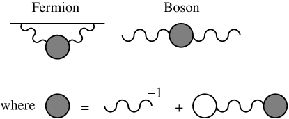
FIG. 1.: All bubble graphs, left, and the resulting self-energies when they are cut, right.

This structure leads to key simplifications which make the calculation of transport coefficients tractable without an expansion in $g^{2}N_{\rm f}$ small. Since the fermions only couple to $O(1)$ gauge boson degrees of freedom, the fermionic self-energy is $O(g^{2})\sim O(1/N_{\rm f})\ll 1$. This behavior is clear at one loop, but it is also true to all orders in loops. The easiest way to see this is to draw all bubble diagrams which appear in the theory at $O(N_{\rm f}^{0})$, which are illustrated in Fig. 1. Since any self-energy can be generated by cutting one line in a bubble diagram, the fermionic self-energy to the order of interest can be obtained from this set of bubble diagrams.

The smallness of the fermionic self-energy means that fermions are almost free particles. In particular, the imaginary part of the fermionic self-energy is $\sim 1/N_{\rm f}$ for all momenta. Therefore, there is a sharp quasi-particle mass shell for fermions, even if $g^{2}N_{\rm f}$ is parametrically $O(1)$. Fermions propagate freely over very long distances, undergoing occasional collisions with mean separation $\sim N_{\rm f}/T$. For this reason a kinetic theory description of the fermions is reliable, with $O(g^{2}\sim 1/N_{\rm f})$ (and therefore negligible) corrections.

A kinetic description of fermions only, without including gauge bosons as kinetic degrees of freedom, is also sufficient. This is so because fermions dominate the observables of interest in this paper, the stress-energy $T_{\mu\nu}$ and all fermionic number currents, simply because there are $O(N_{\rm f})$ times as many fermionic as gauge degrees of freedom.

The other key simplification is that, at leading order, the fermion and gauge boson self-energies each have a very simple structure. The gauge boson propagator is, at $O(N_{\rm f}^{0})$ but to all orders in $g^{2}N_{\rm f}$, given by re-summing a one loop fermionic self-energy,

$$D_{\mu\nu}^{-1}=D_{\mu\nu,{\rm free}}^{-1}-\Pi_{\mu\nu}({\rm 1\;loop})\,.$$ (1)

This should be clear from Fig. 1. The fermionic self-energy is gotten by putting the resummed gauge boson propagator into the self-energy diagram shown in Fig. 1. At leading order in a $1/N_{\rm f}$ expansion the fermionic lines needed to compute $\Pi_{\mu\nu}$ in Eq. (1), and the fermionic line appearing in the fermionic self-energy, are free theory lines.

These simplifications will be sufficient so that we will be able to solve for the transport coefficients within kinetic theory, without uncontrolled approximations. Our method for solving for the transport coefficients follows very closely our previous work [20], except that we will not need to make a leading log approximation of scattering processes, but will be able to treat them in a complete way (at leading order in $1/N_{\rm f}$). Some integrals need to be done numerically and the momentum dependence of the departure from equilibrium has to be modeled with a several parameter Ansatz, but for both approximations the error in the treatment can be made arbitrarily small with sufficient numerical effort; modest effort drives relative errors to $0.1\%$.

The large $N_{\rm f}$ theory has a technical problem, which is that it does not exist, because the gauge boson propagator exhibits a Landau pole at finite $Q^{2}$. However, provided $Q_{\rm Landau}\gg T$ (say, at least $40T$), this problem is only manifested at energy scales which the thermal bath probes exponentially rarely. It is therefore irrelevant to the thermal physics we study. Avoiding Landau pole physics restricts somewhat the range of $g^{2}N_{\rm f}$ we can consider, but it is not a severe restriction; the perturbative expansion is still not guaranteed to be well behaved at the largest values of $g^{2}N_{\rm f}$ which satisfy the above criterion.

An outline of the paper is as follows. We discuss how the transport coefficients are to be computed via kinetic theory in Sec. II. The most complicated feature of the kinetic theory is the collision integral, which is discussed in Sec. III, with some details relegated to two appendices. Our exact (at leading order in $1/N_{\rm f}$) results for transport coefficients appear in Sec. IV. Then, Sec. V discusses how the HTL approximation can be used in the calculation to obtain the result to leading order in $g^{2}N_{\rm f}$, using a simpler scattering matrix element. It presents a comparison of the leading order result with the exact result. Finally, there is a conclusion, Sec. VI. A very brief summary of the conclusion is that, at relatively weak coupling, the leading order calculation works extremely well; but at couplings relevant for even the highest energy heavy ion collisions currently being considered, a full leading order treatment is at best a factor of 2 estimate, because of severe renormalization scale uncertainty. The renormalization point suggested by dimensional reduction turns out to do surprisingly well at large $N_{\rm f}$; but it is difficult to extrapolate, whether this will occur more generally.

II Transport Coefficients and Kinetic Theory

A Transport coefficients

The equilibrium state of a plasma, or any system, is determined by the densities of all conserved quantities. For the theory we consider, massless QED or QCD with many Dirac fermion species, the conserved quantities are the energy-momentum tensor, fermionic particle number, and the charges under SU($N_{\rm c}$)$\times$SU($N_{\rm c}$) flavor rotations. In the grand canonical ensemble these are determined by the timelike inverse temperature 4-vector $\beta_{\mu}$ and various chemical potentials $\mu^{s}$ (with $s$ a combined species and spin label). Here $\beta_{\mu}$ determines both the temperature $1/T=\beta=\sqrt{-\beta_{\mu}\beta^{\mu}}$ and the velocity of flow $u_{i}=\beta_{i}/\beta_{0}$ of the fluid, and the $\mu^{s}$ determine the values of the conserved particle numbers. [Note that we use a $({-}{+}{+}{+})$ index metric throughout, so timelike 4-vectors have negative squares.]

The hydrodynamic regime is the regime where the densities of conserved quantities vary slowly enough in space that the local state at each point can be described up to small corrections by the equilibrium configuration, but with spacetime dependent $\beta_{\mu}$ and $\mu^{s}$. Transport coefficients are defined in terms of the departure from equilibrium, due to the gradients of conserved quantities, and are related to entropy production and the damping away of the spatial inhomogeneity. In particular, viscosities are defined by the difference between the equilibrium and actual stress energy tensor. If in equilibrium and in the (local) rest frame ${\bf u}(x)=0$ the stress tensor is given by $T_{ij}=\delta_{ij}{\cal P}$ (${\cal P}$ the pressure, a function of $\beta_{\mu}$ and the $\mu^{s}$), then when ${\bf u}$ has gradients, $T_{ij}$ is given to lowest order in the gradients of ${\bf u}$ by

$$T_{ij}=\delta_{ij}{\cal P}-\eta\Big{[}\nabla_{i}u_{j}+\nabla_{j}u_{i}-\frac{2}{3}\delta_{ij}\nabla_{l}u_{l}\Big{]}-\zeta\delta_{ij}\nabla_{l}u_{l}\,,$$ (2)

with $\eta$ the shear viscosity and $\zeta$ the bulk viscosity. (Both are functions of $\beta$ and the $\mu^{s}$.) Evaluating bulk viscosity is quite complicated because it involves the physics of particle number changing processes [6]; we will not treat it here, but estimate parametrically that $\zeta\sim N_{\rm f}^{2}T^{3}$, times a dimensionless function of $g^{2}N_{\rm f}$, in this theory.

The other transport coefficient we consider is number diffusion. The diffusion constant for a conserved current $j_{\mu}$ is defined by the constitutive relation (in the frame ${\bf u}=0$)

$$j_{i}=-D\nabla_{i}j_{0}\,.$$ (3)

If we choose to consider a U(1) theory where all fermions have the same U(1) gauge charge, the total fermionic particle number is constrained, in equilibrium, to be zero. However this restriction does not apply for nonabelian gauge theories, or for the other conserved particle numbers. There are therefore a large number of fermionic number densities with diffusion constants we can consider. In general we should permit the diffusion “constant” to be a matrix in the flavor space of conserved currents. However, to leading order in $N_{\rm f}$ all the diffusion constants prove to be the same, so we will ignore this complication. In the U(1) theory, the diffusion of the total fermionic number density is related to the behavior of infrared electric fields and turns out to give the electrical conductivity; this is discussed more in [20].

B Kinetic theory

The stress tensor arises predominantly from fermionic degrees of freedom, simply because there are $O(N_{\rm f})$ of them, and only $O(1)$ gauge degrees of freedom. Naturally, fermionic currents and densities are determined entirely by the fermionic degrees of freedom. Furthermore, because $g^{2}\sim 1/N_{\rm f}$ is very small, the stress-energy and fermionic currents are determined up to small correction by the fermionic two point functions. Hence it is sufficient, to determine transport coefficients to leading order in $1/N_{\rm f}$, to determine the departure from equilibrium of the fermionic two point function. This is precisely the purpose of kinetic theory, so we turn to it next.

It is not our intention in this paper to derive kinetic theory; we feel that the groundwork has been adequately established elsewhere [22, 23, 6]. However, we will outline the parametric argument that kinetic theory is applicable to the current problem. The easiest way to see that a kinetic theory description is possible is to write down all bubble graphs which appear at $O(N_{\rm f}^{1})$ and at $O(N_{\rm f}^{0})$. These are shown in Fig. 1. Cutting one line in a graph gives the propagator to the order of interest. The leading order diagram is an undecorated fermion loop. Cutting it gives the bare fermionic propagator, which tells us that the fermionic propagator is at leading order a free propagator. (This is obvious since the lowest order fermionic self-energy is $O(g^{2}\sim 1/N_{\rm f})$.) Cutting the $O(N_{\rm f}^{0})$ graph on a gauge boson line shows that the gauge boson propagator is at leading order a resummation of one loop self-energy insertions, while cutting on a fermionic line shows that the leading fermionic self-energy correction involves such a resummed gauge boson line and a bare fermionic line. (The gauge boson self-energy is large and requires resummation because $N_{\rm f}$ different fermions can run in the loop, and we must treat $g^{2}N_{\rm f}$ as $O(1)$.)

This means that it will be possible to use kinetic theory to determine transport coefficients in this theory, with errors suppressed by $1/N_{\rm f}$, provided that we carry out a resummation of the gauge boson self-energy wherever a gauge boson line appears in any process. It is incorrect and unnecessary to include gauge bosons as degrees of freedom of the kinetic theory; incorrect because they do not have a sharp mass shell, and unnecessary because there are so few gauge boson degrees of freedom, so they have a negligible role both in carrying conserved quantities and as out states in scattering processes.

The set of scattering processes needed in the kinetic theory, neglecting $1/N_{\rm f}$ corrections, is very small, and it will turn out that the scattering processes are simple enough that they can be treated without uncontrolled approximations. Note that the large $N_{\rm f}$ expansion is much more restrictive than the large $N_{\rm c}$ expansion in QCD; whereas at large $N_{\rm c}$ all planar diagrams survive at leading order, at large $N_{\rm f}$ the structure even of the first subleading diagrams is still very simple. In particular it is only at $O(1/N_{\rm f})$ that diagrams containing nonabelian 3-point vertices first appear. This is why, at the order of interest, there is no difference between treating QCD and QED.

Another requirement for a kinetic treatment to be useful is that it is possible to expand the space dependence of the two point function in gradients and drop terms with more than 1 gradient. This is permissible in determining transport coefficients because they by definition describe the plasma’s response to an arbitrarily slowly varying disturbance. In the case of shear viscosity, we consider an arbitrarily slowly varying, divergenceless velocity field. In the case of fermionic particle number diffusion, we consider a slowly spatially varying chemical potential $\mu$, which we take to be small, $\beta\mu\ll 1$. Slowly varying means that the gradients must vary on scales well larger than $\beta N_{\rm f}$.

In this regime we can write down a Boltzmann equation for the fermionic population function (1 particle density matrix) $f^{s}({\bf p},{\bf x},t)$ (with $s$ a spin, flavor, particle/anti-particle index), describing its time evolution:

$$\left[{\partial\over\partial t}+{\bf v}_{\bf p}\cdot{\partial\over\partial{\bf x}}+{\bf F_{\rm ext}}\cdot{\partial\over\partial{\bf p}}\right]f^{s}({\bf p},{\bf x},t)=-C[f]\,,$$ (4)

with ${\bf v}_{\bf p}=\hat{\bf p}$ the particle velocity, $F_{\rm ext}$ an external force (if any), and $C$ the collision integral, discussed more below. Neither shear viscosity nor fermionic number diffusion require including $F_{\rm ext}$, so we drop it henceforth. The collision integral is zero for the equilibrium population function

$$f_{0}^{s}({\bf p})=\Big{[}1+\exp(-\beta_{\mu}p^{\mu}-q^{s}\beta\mu)\Big{]}^{-1}\,,$$ (5)

where $q^{s}$ is the charge of species $s$ under the fermionic number under consideration. The sign of $q^{s}$ is opposite between particle and anti-particle. We will expand in the small departure from equilibrium, which is justified since the size of the spatial scale of variation of $\beta_{\mu}({\bf x})$, $\mu({\bf x})$ is very large;

$$f^{s}({\bf p},{\bf x},t)=f_{0}({\bf p},\beta({\bf x}),\mu({\bf x}))+f_{0}(1{-}f_{0})\;\delta f^{s}({\bf p},{\bf x},t)\,.$$ (6)

$\delta f^{s}$ is the quantity we are after, since the transport coefficients are determined by it. The nonequilibrium piece of the stress tensor is

$$T_{ij}-\delta_{ij}{\cal P}=\sum_{s}\int\frac{d^{3}p}{(2\pi)^{3}}|{\bf p}|\>\hat{p}_{i}\hat{p}_{j}\,f_{0}(1{-}f_{0})\;\delta f^{s}({\bf p})\,,$$ (7)

and the current of species $s$ is

$$j_{i}^{s}=\sum\int\frac{d^{3}p}{(2\pi)^{3}}\,q^{s}\,\hat{p}_{i}\,f_{0}(1{-}f_{0})\;\delta f^{s}({\bf p})\,,$$ (8)

with the sum over particle and anti-particle. Hence, determining $\delta f$ in terms of $\partial_{i}u_{j}$ and $\nabla_{i}\mu$ will determine the transport coefficients.

Since the gradient is taken small, $\delta f\ll f_{0}$ and we can linearize in $\delta f$. The spatial variation, both of $f_{0}$ and $\delta f$, is slow; so we need only keep the gradient terms on the LHS of Eq. (4) when they act on $f_{0}$. The time derivative term is also irrelevant [20]. The LHS of the Boltzmann equation becomes

$$\beta f_{0}({\bf p})[1{-}f_{0}({\bf p})]\left[q^{s}\hat{p}_{i}\nabla_{i}\mu^{s}+\frac{|{\bf p}|}{2}\left(\hat{p}_{i}\hat{p}_{j}-\frac{1}{3}\delta_{ij}\right)\left(\nabla_{i}u_{j}+\nabla_{j}u_{i}-\frac{2}{3}\delta_{ij}{\bf\nabla}\cdot{\bf u}\right)\right]\,.$$ (9)

In writing the term involving $\nabla_{i}u_{j}$ in this form we have used the restriction that we only consider divergenceless flow, ${\bf\nabla}\cdot{\bf u}=0$. The linearized collision operator is rotationally invariant, so $\delta f$ will have the same angular dependence on $\hat{\bf p}$ as the left hand side. Since the two terms have different angular dependence (the chemical potential involves an $\ell=1$ spherical harmonic while the velocity gradient involves an $\ell=2$ spherical harmonic), the two problems can be treated separately. We will define a particle’s “charge” $q$ to be $q^{s}$ for the case of number diffusion and $|{\bf p}|$ for the case of shear viscosity. It is also convenient to introduce [20]

$$I_{i\cdots j}(\hat{\bf p})\equiv\cases{\;\hat{p}_{i}\,,\vphantom{\Big{|}}&\mbox{(diffusion)}\cr\sqrt{3\over 2}\,(\hat{p}_{i}\hat{p}_{j}-{1\over 3}\delta_{ij})\,,&\mbox{(shear viscosity)}\cr}$$ (10)

and

$$X_{i\cdots j}(x)\equiv\cases{\;\nabla_{i}\,\mu\,,&\mbox{(diffusion)}\cr\frac{1}{\sqrt{6}}\left(\nabla_{i}u_{j}+\nabla_{j}u_{i}-{2\over 3}\delta_{ij}\nabla\cdot{\bf u}\right).&\mbox{(shear viscosity)}\cr}$$ (11)

$X_{i\cdots j}$ parameterizes the source for the departure from equilibrium. The LHS of Eq. (9) is proportional to $X_{i\cdots j}(x)I_{i\cdots j}(\hat{\bf p})$. The normalization is chosen so that $I_{i\cdots j}(\hat{\bf p})I_{i\cdots j}(\hat{\bf p})=1$. For two general vectors ${\bf p}$ and ${\bf k}$,

$$I_{i\cdots j}(\hat{\bf p})I_{i\cdots j}(\hat{\bf k})=P_{\ell}(\hat{\bf p}\cdot\hat{\bf k})\,,$$ (12)

with $P_{\ell}$ the $\ell$’th Legendre polynomial, and with $\ell$ the spherical harmonic represented by $I_{i\cdots j}$, which is the same as the number of indices $I_{i\cdots j}$ carries.

Rotational invariance of the collision integral ensures that we can write the departure from equilibrium as

$$\delta f^{s}({\bf p},{\bf x})=\beta^{2}X_{i\cdots j}(x)\chi^{s}_{i\cdots j}({\bf p})\,,\qquad\chi^{s}_{i\cdots j}({\bf p})=I_{i\cdots j}(\hat{\bf p})\chi^{s}(|{\bf p}|)\,.$$ (13)

The function $\chi^{s}(|{\bf p}|)$ depends only on the magnitude of the momentum and characterizes the departure from equilibrium of the plasma. It has the size of the source for departure from equilibrium, $X_{i\cdots j}$, and the angular dependence of the departure, $I_{i\cdots j}$, scaled out from it, and is the most convenient variable in terms of which to write the Boltzmann equation. Defining a “normalized source” for the departure from equilibrium,

$$S^{s}_{i\cdots j}({\bf p})\equiv-T\,q^{s}f_{0}({\bf p},x)[1{-}f_{0}({\bf p},x)]\>I_{i\cdots j}(\hat{\bf p})\,,$$ (14)

(where again, for diffusion $q^{s}$ is defined above and for shear viscosity $q^{s}=|{\bf p}|$), the linearized Boltzmann equation, Eq. (9), becomes

$$S^{s}_{i\cdots j}({\bf p})=\left({\cal C}\chi_{i\cdots j}\right)^{s}({\bf p})\,.$$ (15)

The exact form of the collision operator ${\cal C}$ will be presented below. The solution $\chi_{i\cdots j}$ is simply related to the transport coefficients [20]. Introducing the inner product (under which the collision operator ${\cal C}$ is Hermitian and positive semidefinite)

$$\Big{(}f,g\Big{)}\equiv\beta^{3}\sum_{a}\int\frac{d^{3}p}{(2\pi)^{3}}\,f^{a}({\bf p})\,g^{a}({\bf p})\,,$$ (16)

and considering the case of a fermionic number where all fermions have $q^{2}=1$, using Eq. (7) and Eq. (8) and the definitions of the transport coefficients leads to

$$\eta = \frac{1}{15}\Big{(}\chi_{ij},{\cal C}\chi_{ij}\Big{)}\,,$$ (17)

$$D = \frac{1}{N_{\rm f}T^{2}}\Big{(}\chi_{i},{\cal C}\chi_{i}\Big{)}\,.$$ (18)

The coefficient in front of $D$ would be $1/3$, except that $D$ is defined as $-j_{i}/\nabla_{i}j_{0}$, not $-j_{i}/\nabla_{i}\mu$. The ratio $j_{0}/\mu$ is the charge susceptibility, and for small $\mu$ a simple calculation gives $j_{0}/\mu=N_{\rm f}T^{2}/3$.

C Variational method

The departure from equilibrium $\chi(|{\bf p}|)$ is determined by Eq. (15), which is an integral equation. (This will become clear when we write the form of the collision integral explicitly, Eq. (27) below.) Integral equations are difficult to solve unless the integration kernel ${\cal C}$ has a particularly simple form, which is not the case for us. Abandoning an exact solution, we can still get a very accurate solution for $\chi$, and a more accurate determination of $\eta$ and $D$, by expressing the problem as a variational one, writing down a trial function for $\chi(|{\bf p}|)$ and solving for a finite number of variational coefficients. The accuracy can then be improved, in principle without limit, by enlarging the basis of variational functions considered. This technique constitutes a controlled approximation, meaning that it can be made arbitrarily accurate. It does not in practice limit the accuracy with which we can extract transport coefficients. This strategy has a very long history in the solution of kinetic equations, see for instance [24]. Here we follow the approach of [20]. Eq. (15) is satisfied at the variational extremum of

$$Q(\chi)\equiv\Big{(}S_{i\cdots j}\,,\,\chi_{i\cdots j}\Big{)}-\frac{1}{2}\Big{(}\chi_{i\cdots j}\,,\,{\cal C}\chi_{i\cdots j}\Big{)}\,,$$ (19)

and the value of the extremum is

$$Q_{\rm max}=\frac{1}{2}\Big{(}\chi_{i\cdots j}\,,\,{\cal C}\chi_{i\cdots j}\Big{)}\,.$$ (20)

This extremal value is simply related to the transport coefficients, presented in Eq. (18). Since the transport coefficients correspond to the value of $Q$ at a maximum, the error in their determination is quadratic in the error between a trial $\chi$ and the optimal $\chi$. Hence, extremizing over a suitably flexible Ansatz for $\chi$ will give a very accurate value for the transport coefficients. Following [20], we consider the Ansatz

$$\chi^{s}(p)=\sum_{m=1}^{N}a_{m}q^{s}\phi^{(m)}(p)\,,$$ (21)

with $p=|{\bf p}|$ and $\phi^{(m)}$ some set of test functions. Our choice is

$$\phi^{(m)}(p)=\frac{(p/T)^{m}}{(1+p/T)^{N-1}}\,,\qquad m=1,\ldots,N\,,$$ (22)

but other choices also work and lead to the same numerical answer. Note that the $\phi^{(m)}$ for a small value of $N$ are each linear combinations of the $\phi^{(m)}$ for a larger $N$, so increasing $N$ strictly increases the span of the Ansatz.

Inserting this Ansatz for $\chi$ into Eq. (19) turns it into a quadratic equation for the coefficients $a_{m}$;

$$\tilde{Q}[\{a_{m}\}]=\sum_{m=1}^{N}a_{m}\,\tilde{S}_{m}-{\textstyle{1\over 2}}\sum_{m,n=1}^{N}a_{m}\,\tilde{C}_{mn}\,a_{n}\,,$$ (23)

with $\tilde{S}_{m}$ given by $\tilde{S}_{m}\equiv\Big{(}S_{i\cdots j},q\phi_{i\cdots j}^{(m)}\Big{)}$, and similarly $\tilde{C}_{mn}\equiv\Big{(}q\phi_{i\cdots j}^{(m)},\,{\cal C}q\phi_{i\cdots j}^{(n)}\Big{)}$, where $\phi^{(m)}_{i\cdots j}({\bf p})\equiv I_{i\cdots j}(\hat{\bf p})\phi^{(m)}(p)$. Maximizing $\tilde{Q}$ is now a trivial linear algebra exercise which gives $a=\tilde{C}^{-1}\,\tilde{S}$ and

$$Q_{\rm max}=\frac{1}{2}\tilde{S}^{\top}\,\tilde{C}^{-1}\,\tilde{S}\,,$$ (24)

where $a=||a_{m}||$ and $\tilde{S}=||\tilde{S}_{m}||$ are the $N$-component coefficient and source vectors, respectively, in the chosen basis, and $\tilde{C}\equiv||\tilde{C}_{mn}||$ is the (truncated) collision matrix. The determination of transport coefficients then hinges on the accurate evaluations of the integrals $\Big{(}S_{i\cdots j},q\phi_{i\cdots j}^{(m)}\Big{)}$ and $\Big{(}q\phi_{i\cdots j}^{(m)},\,{\cal C}q\phi_{i\cdots j}^{(n)}\Big{)}$. The integral involved in determining $\tilde{S}_{m}$ is 1 dimensional and is easy to evaluate, quickly and accurately, by numerical quadratures; we do not discuss it further. Evaluating $\tilde{C}_{mn}$ is the topic of the next section. However it is already possible to determine the power of $N_{\rm f}$ which will appear in the final answer. The quantity $\tilde{S}$ contains a sum over all species but no powers of the coupling constant, so it is $O(N_{\rm f})$. The collision integral, since it arises from an $O(1)$ bubble diagram, must be $\tilde{C}_{mn}\sim N_{\rm f}^{0}$. The appropriate powers of $T$ follow easily on dimensional grounds. Therefore $\eta\propto N_{\rm f}^{2}T^{3}$, and $D\propto N_{\rm f}/T$ (because there is an explicit negative power of $N_{\rm f}$ in Eq. (18)).

III Collision integral

A Relevant diagrams

To make more progress we must analyze what collision processes are important in this theory. They are given by cutting the fermionic self-energy diagram of Fig. 1, see Fig. 2. Two scattering processes are important, $t$ channel scattering from a particle or anti-particle and $s$ channel annihilation and creation of a new pair. The external lines in these processes may all be treated as massless, on-shell particles, with uncorrected dispersion relations, since the self-energy of the fermion is $O(g^{2}\sim 1/N_{\rm f})$. This is not so for the gauge boson propagator appearing in the diagram, which must be treated with care.

FIG. 2.: Scattering processes which must be considered at leading order .

Note that only $2\leftrightarrow 2$ processes appear in the collision integral to the order of interest, and that the external lines are all fermions. The set of diagrams required is much simpler than the set which are needed at leading order in $g$ when not adopting the large $N_{\rm f}$ expansion. In that case, Compton scattering and annihilation to gauge bosons are already present at leading logarithmic order [20], and at leading order interference diagrams between external leg assignments of the $s$ and $t$ channel processes are also present. Similarly, in the current context, bremsstrahlung emission is also suppressed. These “notable for their absence” diagrams are summarized in Fig. 3. In each case there is a clear power counting reason for the diagram’s absence. Interference between external legs is only possible when all external lines are of the same species; but this only occurs in $1/N_{\rm f}$ of scattering events. Similarly, Compton scattering or annihilation to gauge bosons involve a sum over only one, not two, fermionic species indices. Another way to see the suppression of these processes is to consider what bubble graph must be cut to produce them; this is also shown in Fig. 3, and in each case the bubble diagram is $O(N_{\rm f}^{-1})$.

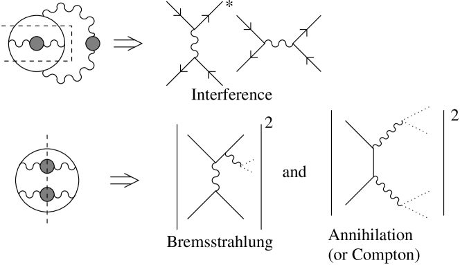
FIG. 3.: Scattering processes which may be important at leading order in the coupling $g$, when we do not expand in $N_{\rm f}$, but which are $N_{\rm f}$ suppressed and can be neglected here. Dashed lines on the bubble graphs show where they are cut to give the diagrams presented. Dotted lines in the scattering processes indicate that gauge bosons are not propagating states in the kinetic theory, and we must consider the process including the states a gauge boson eventually scatters against or decays into.

B Form of $\tilde{C}_{mn}$

Since only $2\leftrightarrow 2$ processes are important, the collision integral can be written [20]

$$({\cal C}\chi_{i\cdots j})^{a}({\bf p}) = \frac{1}{2}\sum_{bcd}\int\frac{d^{3}{\bf k}d^{3}{\bf p}^{\prime}d^{3}{\bf k}^{\prime}}{(2\pi)^{9}16pkp^{\prime}k^{\prime}}(2\pi)^{4}\delta^{3}({\bf p}+{\bf k}-{\bf p}^{\prime}-{\bf k}^{\prime})\delta(p+k-p^{\prime}-k^{\prime})$$ (27)

$$\qquad\quad\times\left|{\cal M}^{ab}_{cd}({\bf p},{\bf k},{\bf p}^{\prime},{\bf k}^{\prime})\right|^{2}f_{0}^{a}(p)\,f_{0}^{b}(k)[1{-}f_{0}^{c}(p^{\prime})][1{-}f_{0}^{d}(k^{\prime})]$$

$$\qquad\quad\times\Bigl{[}\chi^{a}_{i\cdots j}({\bf p})+\chi^{b}_{i\cdots j}({\bf k})-\chi^{c}_{i\cdots j}({\bf p}^{\prime})-\chi^{d}_{i\cdots j}({\bf k}^{\prime})\Bigr{]}\,.$$

Our notation is that the incoming momenta are ${\bf p}$ and ${\bf k}$ and the outgoing momenta are ${\bf p}^{\prime}$ and ${\bf k}^{\prime}$; and as before, $k=|{\bf k}|$, and so forth. ${\cal M}^{ab}_{cd}({\bf p},{\bf k},{\bf p}^{\prime},{\bf k}^{\prime})$ is the matrix element (in relativistic normalization) for $(ab)$ to go to $(cd)$. We have already enforced on-shell delta functions on the external 4-momenta using free massless dispersion relations, so the energies of the external particles equal the magnitudes of their momenta. The leading factor of $(1/2)$ corrects for the $c\leftrightarrow d$ double counting of the sum, or for the outgoing symmetry factor when $c=d$.

The quantity we want is $\tilde{C}_{mn}$, that is, Eq. (27) with $\chi_{ij}^{s}$ replaced with $q^{s}\phi^{(m)}_{i\cdots j}$, multiplied by $q^{a}\phi^{(n)}_{i\cdots j}({\bf p})$, integrated over ${\bf p}$, and summed over $a$. The resulting phase space integral and matrix element are symmetric on interchange of the $(abcd)$ indices, so we can also symmetrize the $\phi$ factors, yielding

$$\Big{(}q\phi^{(m)}_{i\cdots j}\,,\,{\cal C}q\phi^{(n)}_{i\cdots j}\Big{)} = \frac{\beta^{3}}{8}\sum_{abcd}\int\frac{d^{3}{\bf p}d^{3}{\bf k}d^{3}{\bf p}^{\prime}d^{3}{\bf k}^{\prime}}{(2\pi)^{12}16pkp^{\prime}k^{\prime}}(2\pi)^{4}\delta^{3}({\bf p}+{\bf k}-{\bf p}^{\prime}-{\bf k}^{\prime})\delta(p+k-p^{\prime}-k^{\prime})$$ (31)

$$\qquad\quad\times\left|{\cal M}^{ab}_{cd}({\bf p},{\bf k},{\bf p}^{\prime},{\bf k}^{\prime})\right|^{2}f_{0}^{a}(p)\,f_{0}^{b}(k)[1{-}f_{0}^{c}(p^{\prime})][1{-}f_{0}^{d}(k^{\prime})]$$

$$\qquad\quad\times\Bigl{[}q^{a}\phi^{(m)}_{i\cdots j}({\bf p})+q^{b}\phi^{(m)}_{i\cdots j}({\bf k})-q^{c}\phi^{(m)}_{i\cdots j}({\bf p}^{\prime})-q^{d}\phi^{(m)}_{i\cdots j}({\bf k}^{\prime})\Bigr{]}$$

$$\qquad\quad\times\Bigl{[}q^{a}\phi^{(n)}_{i\cdots j}({\bf p})+q^{b}\phi^{(n)}_{i\cdots j}({\bf k})-q^{c}\phi^{(n)}_{i\cdots j}({\bf p}^{\prime})-q^{d}\phi^{(n)}_{i\cdots j}({\bf k}^{\prime})\Bigr{]}\,.$$

It is clear from this expression that ${\cal C}$ is positive semidefinite. For $\ell\neq 0$, it is in fact positive definite.

The matrix element gets 3 contributions; the $s$ channel contribution, the $t$ channel contribution for scattering of like sign (both particle or both anti-particle) fermions, and the $t$ channel contribution for scattering of opposite sign fermions (a particle and an anti-particle). The matrix element for the $s$ channel process, summed over all species indices $(abcd)$ and including the symmetry factor of $(1/8)$, is

$${\rm s\;channel:}\quad\frac{1}{8}\sum_{abcd}\left|{\cal M}^{ab}_{cd}\right|^{2}=4(g^{2}N_{\rm f})^{2}\;\raisebox{8.00003pt}{\mbox{``}}\!\!\left(\frac{t^{2}+u^{2}}{s^{2}}\right)\!\!\raisebox{8.00003pt}{\mbox{''}}\>\,,$$ (32)

for the U(1) theory. We discuss the nonabelian generalization in the next section. The meaning of “[$t^{2}+u^{2}$$/s^{2}$]” is a quantity which equals this (with $s,t,u$ the usual Mandelstam variables) in the small $g^{2}N_{\rm f}$ limit, and is given in complete detail in Appendix B Eq. (B9). The expression for $t$ channel, like sign scattering is

$${\rm t\;channel\;like\;sign:}\quad\frac{1}{8}\sum_{abcd}\left|{\cal M}^{ab}_{cd}\right|^{2}=4(g^{2}N_{\rm f})^{2}\;\raisebox{8.00003pt}{\mbox{``}}\!\!\left(\frac{s^{2}+u^{2}}{t^{2}}\right)\!\!\raisebox{8.00003pt}{\mbox{''}}\>\,.$$ (33)

The expression for opposite sign scattering is identical. Again, the quantity “[$s^{2}+u^{2}$$/t^{2}$]” equals this in the small $g^{2}N_{\rm f}$ limit, but is given by a more complicated expression presented in Appendix B, Eq. (B12).

C Doing the integrals

To compute transport coefficients it remains to perform the integrals presented in Eq. (31). There is a 12 dimensional integral to perform. Four of the integrals will be performed by the energy-momentum conserving delta functions, and three are trivial because the way we structured Eq. (9) makes Eq. (31) invariant under global rotations. This leaves 5 integrals. Appendix A shows two nice ways of parametrizing these remaining integrals. One way, due to [13], is convenient for $t$ channel exchange, and another is convenient for $s$ channel exchange.

We can write Eq. (31) as a sum of two 5 dimensional integrals, one containing the $s$ channel contribution to $|{\cal M}|^{2}$ and the other containing the $t$ channel contributions, by using Eq. (A6) and Eq. (A20). The matrix elements are given by Eq. (32) with Eq. (B9), and twice Eq. (33) with Eq. (B12). The product of $\phi$ functions is evaluated for shear viscosity using

$$|{\bf p}|\phi^{(m)}_{ij}(\hat{\bf p})|{\bf k}|\phi^{(n)}_{ij}(\hat{\bf k})=pk\phi^{(m)}(p)\phi^{(n)}(k)P_{2}(\cos\theta_{pk})\,,$$ (34)

and similarly for the other terms when the product of $\phi$’s is expanded. Here $P_{2}(x)=(3x^{2}-1)/2$ is the second Legendre polynomial, and all the cosines of angles are given in Appendix A. For both the $s$ and $t$ channel part of the scattering integral, there is an integration over an azimuthal angle $\phi$ which can be done analytically, leaving a 4 dimensional integral, over the frequency $\omega$ and momentum $q$ carried by the gauge boson line and two external momenta. The integrand is long and unenlightening and can be obtained from the equations listed above. We perform it by numerical quadratures using adaptive mesh refinement methods. The accuracy with which the integrals can be performed limits the accuracy of the determination of the transport coefficients, but it is not too difficult to achieve $0.1\%$ accuracy in the finally determined transport coefficients, for the full range of the coupling constant $g^{2}N_{\rm f}$ that we consider. Note that, besides the explicit $g^{2}N_{\rm f}$ dependence of Eq. (32) and Eq. (33), there is also quite complicated $g^{2}N_{\rm f}$ dependence in the matrix elements because of the gauge boson self-energies. Therefore the full integration must be re-performed for every value of $g^{2}N_{\rm f}$ under study. Note also that $g^{2}N_{\rm f}$ requires (vacuum) renormalization. We regularize using the $\overline{\hbox{MS}}$ scheme. We also choose the renormalization point $\bar{\mu}$ to be the “dimensional reduction” value [25] $\bar{\mu}_{\rm DR}=\pi T\exp(-\gamma_{\rm E})$, with $\gamma_{\rm E}=.577\ldots$ the Euler-Mascheroni constant. This choice is arbitrary and represents a choice in the presentation of the results only. Its motivation is that, at this renormalization point only, the free energy of an infrared electromagnetic field is given by $\int d^{3}x({\bf E}^{2}+{\rm B}^{2})/2$.

We also cannot treat arbitrarily large $g^{2}N_{\rm f}$ because the presence of the Landau pole in the theory becomes problematic. Requiring that the Landau pole occur further into the ultraviolet than $|q^{\mu}q_{\mu}|=(40T)^{2}$ requires $g\sqrt{N_{\rm f}}\leq 4.4$. A Landau pole this far in the ultraviolet does not affect our calculation because the contribution to Eq. (31) from integration regions with $|\omega^{2}-q^{2}|$ large enough to encounter the Landau pole is exponentially small. In fact such regions were never sampled by the adaptive integration routine. For $gN_{\rm f}^{1/2}=3$, the energy scale where the pole appears is already above $1000T$.

For the case of fermion number diffusion, there are some additional cancellations which make the structure of the integrand slightly simpler than for shear viscosity. Unlike shear viscosity, the charge $q^{s}$ for number diffusion is opposite for a particle and its anti-particle. Further, the $t$ channel matrix element to scatter from a particle equals the matrix element to scatter from its anti-particle (up to $1/N_{\rm f}$ suppressed corrections). Hence, for $t$ channel exchange, summing on like and opposite sign scatterings cancels all “cross-terms” in Eq. (31) with both $p$ and $k$ line arguments for $\phi$’s. Using also the ${\bf p}\leftrightarrow{\bf k}$ symmetry of the integration, and the fact that the incoming and outgoing particles $a$ and $c$ are the same type and have the same charge, one may substitute

$$\sum_{abcd}|{\cal M}|^{2}(t{\rm\;channel})\Bigl{[}q^{a}\phi^{(m)}_{i}({\bf p})+q^{b}\phi^{(m)}_{i}({\bf k})-q^{c}\phi^{(m)}_{i}({\bf p}^{\prime})-q^{d}\phi^{(m)}_{i}({\bf k}^{\prime})\Bigr{]}$$ (36)

$$\hskip 93.95122pt\times\Bigl{[}q^{a}\phi^{(n)}_{i}({\bf p})+q^{b}\phi^{(n)}_{i}({\bf k})-q^{c}\phi^{(n)}_{i}({\bf p}^{\prime})-q^{d}\phi^{(n)}_{i}({\bf k}^{\prime})\Bigr{]}$$

$$\Rightarrow \sum_{abcd}2|{\cal M}|^{2}(t{\rm\;channel})(q^{a})^{2}\Bigl{[}\phi^{(m)}_{i}({\bf p})-\phi^{(m)}_{i}({\bf p}^{\prime})\Bigr{]}\Bigl{[}\phi^{(n)}_{i}({\bf p})-\phi^{(n)}_{i}({\bf p}^{\prime})\Bigr{]}\,.$$ (37)

For the $s$ channel exchange a similar simplification occurs because in that case $q^{c}=-q^{d}$ but the integral is symmetric on ${\bf p}^{\prime}\leftrightarrow{\bf k}^{\prime}$ (as well as on $({\bf p},{\bf k})\leftrightarrow({\bf p}^{\prime},{\bf k}^{\prime})$); so

$$\sum_{abcd}|{\cal M}|^{2}(s{\rm\;channel})\Bigl{[}q^{a}\phi^{(m)}_{i}({\bf p})+q^{b}\phi^{(m)}_{i}({\bf k})-q^{c}\phi^{(m)}_{i}({\bf p}^{\prime})-q^{d}\phi^{(m)}_{i}({\bf k}^{\prime})\Bigr{]}$$ (39)

$$\hskip 93.95122pt\times\Bigl{[}q^{a}\phi^{(n)}_{i}({\bf p})+q^{b}\phi^{(n)}_{i}({\bf k})-q^{c}\phi^{(n)}_{i}({\bf p}^{\prime})-q^{d}\phi^{(n)}_{i}({\bf k}^{\prime})\Bigr{]}$$

$$\Rightarrow \sum_{abcd}2|{\cal M}|^{2}(s{\rm\;channel})(q^{a})^{2}\Bigl{[}\phi^{(m)}_{i}({\bf p})-\phi^{(m)}_{i}({\bf k})\Bigr{]}\Bigl{[}\phi^{(n)}_{i}({\bf p})-\phi^{(n)}_{i}({\bf k})\Bigr{]}\,.$$ (40)

(The same symmetries were used in [20] to allow a simple leading log calculation of the diffusion constant.) For both the $s$ and $t$ channel integrations, there is an azimuthal integration which is trival, and the two external momentum integrations factor and can be performed separately (rather than being nested). This simplifies somewhat the numerical integrations.

Further, the cancellations just described show that, for number diffusion, the way that the departure from equilibrium in one species evolves decouples from the departure from equilibrium in every other species. This is why all the fermionic diffusion constants are the same, unless the total fermionic number is coupled to a gauged U(1) field.

IV All-orders Results

FIG. 4.: Shear viscosity, computed to all orders in $g^{2}N_{\rm f}$. The renormalization point $\bar{\mu}$ in the $\overline{\hbox{MS}}$ scheme is $\bar{\mu}=\pi e^{-\gamma_{\rm E}}T$, the “dimensional reduction” answer.

FIG. 5.: Diffusion constant, computed to all orders in $g^{2}N_{\rm f}$. The renormalization point is the same as in Fig. 4.

The last two sections describe how the transport coefficients, at leading order in $1/N_{\rm f}$ but all orders in $g^{2}N_{\rm f}$, may be computed for $U(1)$ gauge theory. The results appear in Figures 4 and 5. Here we discuss the results and generalize them to QCD, with $N_{\rm c}\ll N_{\rm f}$ so as not to spoil the expansion we have used.

First we remark that, while there is no “diffusion constant” for the total  fermionic number density when it is coupled to a U(1) gauge field, the would-be diffusion constant instead determines the electric conductivity for the U(1) gauge field [20]:

$$\sigma=\frac{g^{2}N_{\rm f}T^{2}}{3}\,D\,.$$ (41)

Therefore the results in Fig. 5 also constitute a result for the electrical conductivity of this theory. For this interpretation the choice of renormalization constant is essential, since only for $\bar{\mu}=\bar{\mu}_{\rm DR}$ does the free energy density stored in an electric field equal $E^{2}/2$.

In presenting the transport coefficients in Figs 4 and 5, we factor out the leading $g^{-4}$ behavior from the transport coefficients; but there remains nontrivial $g^{2}N_{\rm f}$ dependence. This is because the size of the gauge boson self-energy, relative to the tree gauge propagator, depends on $g^{2}N_{\rm f}$. It is not surprising that this is important for $g^{2}N_{\rm f}\mbox{~{}{\raisebox{1.72218pt}{$>$}} {\raisebox{-2.58334pt}{$\sim$}}~{}}1$. In fact the dependence continues down to arbitrarily small $g^{2}N_{\rm f}$, where the transport coefficient scales as $1/\ln(1/g^{2}N_{\rm f})$. This is because the $t$ channel contribution to the scattering integral, Eq. (31), has a logarithmic small $q$ divergence which is cut off by the presence of a self-energy on the gauge boson line. This is discussed further in the next section.

The results presented in Fig. 4 and Fig. 5 are for U(1) gauge theory. Consider instead a general nonabelian theory, with $N_{\rm f}$ flavors of fermions in a common representation of the group, of dimension $d_{\rm F}$ and with quadratic Casimir $C_{\rm F}$, and trace normalization $T_{\rm F}=C_{\rm F}d_{\rm F}/d_{\rm A}$, with $d_{\rm A}$ the dimension of the adjoint representation. For SU($N_{\rm c}$) gauge theory with fundamental representation fermions, $C_{\rm F}=(N_{\rm c}^{2}-1)/2N_{\rm c}$, $d_{\rm F}=N_{\rm c}$, and $T_{\rm F}=1/2$. The total number of fermionic degrees of freedom is then $4d_{\rm F}N_{\rm f}$, rather than $4N_{\rm f}$ in the U(1) theory. (The 4 is because we consider Dirac fermions; there are two spins, and particle/anti-particle.) Therefore, the sum in Eq. (16) includes $4N_{\rm f}d_{\rm F}$ terms, rather than $4N_{\rm f}$ terms as in the U(1) theory, so $\tilde{S}_{m}$ is multiplied by $d_{\rm F}$. Meanwhile, the gauge field self-energy has the replacement

$$m_{\rm D}^{2}=\frac{g^{2}N_{\rm f}T^{2}}{3}\quad\Rightarrow\quad m_{\rm D}^{2}=\frac{g^{2}(T_{\rm F}N_{\rm f}+T_{\rm A})T^{2}}{3}\simeq\frac{g^{2}T_{\rm F}N_{\rm f}T^{2}}{3}\,.$$ (42)

The expression with $T_{\rm A}$ ($T_{\rm A}=C_{\rm A}$ the adjoint Casimir, $T_{\rm A}=N_{\rm c}$ in SU($N_{\rm c}$) gauge theory) holds generally to leading order in $g^{2}$ in QCD, with the $T_{\rm A}$ term arising from gauge boson loops; in the last expression we have enforced the large $N_{\rm f}$ limit to eliminate this nonabelian term. The group theory coefficient for $\tilde{C}_{mn}$ is $(d_{\rm F}^{2}C_{\rm F}^{2}/d_{\rm A})$. Also, the fermion number susceptibility, which goes into the determination of $D$, is multiplied by $d_{\rm F}$; hence $D$ is smaller by this factor. Therefore, to use the figures to get the transport coefficients for a nonabelian theory, one should interpret the $x$ axis in Fig. 4 as

$$gN_{\rm f}^{1/2}\quad\Rightarrow\quad g(T_{\rm F}N_{\rm f})^{1/2}\,,$$ (43)

and replace the $y$ axis label with

$$\eta\times\frac{g^{4}}{T^{3}}\quad\Rightarrow\quad\eta\times\frac{g^{4}C_{\rm F}^{2}}{d_{\rm A}T^{3}}\,,\qquad D\times g^{4}N_{\rm f}T\quad\Rightarrow\quad D\times\frac{g^{4}N_{\rm f}C_{\rm F}^{2}d_{\rm F}T}{d_{\rm A}}\,.$$ (44)

In SU($N_{\rm c}$) QCD with fundamental fermions, $T_{\rm F}=1/2$, $d_{\rm F}=N_{\rm c}$, and $C_{\rm F}^{2}/d_{\rm A}=(N_{\rm c}^{2}-1)/(4N_{\rm c}^{2})$. In converting $D$ into $\sigma$ using Eq. (41), the $g^{2}$ appearing in that equation should be the U(1) gauge coupling, and there is an additional factor of $d_{\rm F}$,

$$\sigma=\frac{e^{2}d_{\rm F}N_{\rm f}T^{2}}{3}D\,,$$ (45)

with $e$ the fermionic coupling to the U(1) gauge field.

V Leading Order Calculation

One use of our results is to allow a comparison against a leading order calculation which relies on the hard thermal loop expansion. To date, only leading logarithmic results are available. Repeating the analysis of [20] in this context gives at leading logarithmic order

$$D=\frac{91.1725}{N_{\rm f}g^{4}T}\>\times\>\frac{1}{\ln(T/m_{\rm D})+O(1)}\,,\qquad\eta=\frac{61.0727T^{3}}{g^{4}}\>\times\>\frac{1}{\ln(T/m_{\rm D})+O(1)}\,.$$ (46)

To study better the reliability of the HTL expansion, we present here a leading order calculation. We perform it in the spirit of other leading order HTL calculations, which is to say, all self-energies are replaced with just the thermal part of the self-energy in the HTL approximation, wherever that treatment is parametrically justified. Note that the HTL vertices all vanish at leading order in $1/N_{\rm f}$ and are not needed here. In this section and this section alone, we will treat $g^{2}N_{\rm f}$ as a small quantity which can be expanded in parametrically. Equivalently we treat the Debye mass, given by $m_{\rm D}^{2}=g^{2}N_{\rm f}T^{2}/3$, as $m_{\rm D}\ll T$.

It turns out that both the $t$ and $s$ channel exchange parts of the collision integral depend in a nontrivial way on the presence of a self-energy on the gauge boson line. We will discuss each in turn.

A Leading order $t$ channel exchange

It has long been appreciated that there is a subtlety in the $t$ channel exchange process, and that inclusion of a self-energy on the gauge boson lines is necessary, not only to get the correct leading order behavior, but to get a behavior which does not suffer from infrared divergences in the evaluation of the collision integral [13]. This is because of the small denominator provided by the propagator when ${\bf p}-{\bf p}^{\prime}$ is small. As shown in Appendix A, the $t$ channel phase space integrals can be written [13] (Eq. (A6))

$$\frac{\beta^{3}}{2^{9}\pi^{6}}\int_{0}^{\infty}dq\int_{-q}^{q}d\omega\int_{\frac{q-\omega}{2}}^{\infty}dp\int_{\frac{q+\omega}{2}}^{\infty}dk\int_{0}^{2\pi}d\phi\,,$$ (47)

with $p$ and $k$ the energies of the two incoming particles, and $\omega$ and $q$ the energy and momentum carried by the exchanged gauge boson. When the particle energies are $O(T)$ but the exchange momentum is $m_{\rm D}\ll q\ll T$, we can expand in small $q/p$ and simultaneously drop the self-energy effects on the propagators, so that Eq. (B12) becomes

$$\;\raisebox{8.00003pt}{\mbox{``}}\!\!\left(\frac{s^{2}+u^{2}}{t^{2}}\right)\!\!\raisebox{8.00003pt}{\mbox{''}}\>\simeq\frac{s^{2}+u^{2}}{t^{2}}\simeq\frac{8p^{2}k^{2}(1-\cos\theta)^{2}}{q^{4}}\,.$$ (48)

At first sight the integral over $q$ is severely infrared divergent. However, two more powers of $q$ arise from cancellations in the expressions of the form $\Big{[}\phi_{i\cdots j}({\bf p})-\phi_{i\cdots j}({\bf p}^{\prime})\ldots\Big{]}$ in Eq. (31) [20], because ${\bf p}{-}{\bf p}^{\prime}={\bf q}$ is $O(q)$ and $\phi_{i\cdots j}$ is a smooth function of its argument; so the $\phi_{i\cdots j}({\bf p})$ and $\phi_{i\cdots j}({\bf p}^{\prime})$ terms cancel up to an $O(q)$ remainder. Therefore, the $q$ integration is really of the form

$$\sim\int_{\sim m_{\rm D}}^{\sim T}dq\int_{-q}^{q}d\omega\frac{1}{q^{2}}\,,$$ (49)

which is logarithmically sensitive to the $gT$ scale. The upper end of the logarithm is cut off because the expansion $q\ll p$ is no good there. The lower end of the integration range is only cut off by the inclusion of the self-energies in the scattering processes. Therefore it is necessary to include those self-energies to get a finite answer. However, for $m_{\rm D}\ll T$, they only play a role when $q\mbox{~{}{\raisebox{1.72218pt}{$<$}} {\raisebox{-2.58334pt}{$\sim$}}~{}}m_{\rm D}\ll T$, which is clear from the form of the matrix element, given in Eq. (B12).

At leading logarithmic order it is only necessary to determine the coefficient of the log divergence arising from the $m_{\rm D}\ll q\ll T$ momentum range. Such a calculation was carried out in [20], where it was also not necessary to appeal to a large $N_{\rm f}$ expansion. However, a leading order calculation requires a treatment of both the $q\sim m_{\rm D}$ and the $q\sim T$ momentum ranges, as well as the intermediate range. For such a leading order calculation we must perform the full integration presented in Eq. (31). However we may simplify the treatment by replacing the full self-energy on the gauge boson line with its HTL counterpart. That is, we may drop the vacuum contribution to the self-energies, and make the simplifying approximations for the thermal parts which are presented in Eq. (B23). We may do this throughout the integration range of Eq. (31). The vacuum part is uniformly suppressed by $g^{2}N_{\rm f}$ (up to logarithms). At small transfer momenta $q\sim m_{\rm D}$, the corrections to the HTL approximation for the thermal contribution to self-energies is $O(m_{\rm D}^{2}/T^{2}\sim g^{2}N_{\rm f})$, and the approximation is valid. At large momenta $q\sim T$, the HTL approximation is invalid, but the whole thermal self-energy is an $O(g^{2}N_{\rm f})$ correction and is negligible anyway.

Our method for achieving a leading order determination of the integrals in Eq. (31) is therefore to replace the self-energy on the gauge boson line with the HTL self-energy, over the full momentum integration range. The integral is then performed without further approximation (such as expansion in $q\ll p$).

We have also tested the sensitivity to a slight modification of the matrix element, moving the $\cos\phi$ independent piece in Eq. (B12) which is multiplied by $(q^{2}+\tilde{\Pi}_{\rm T})^{-2}$ over to the piece multiplied by $(q^{2}+\tilde{\Pi}_{\rm L})^{-2}$, so appearances of the transverse self-energy coincide with powers of $\cos\phi$. This modification makes an $O(g^{2}N_{\rm f})$ change because the piece moved is $O(g^{2}N_{\rm f})$ suppressed where the difference in self-energies matters. It coincides with the separation between transverse and longitudinal self-energies presented in [14], and is the easiest thing to implement, especially if scatterings with gauge bosons are important (in a nonabelian theory and not at large $N_{\rm f}$). We find the difference is relatively small, comparable to the difference between the leading order at the dimensional reduction renormalization point and the all orders answer. This is not the procedure we used to get the results presented in the figures to follow.

B Leading order $s$ channel exchange

Naively, the $s$ channel exchange contribution to Eq. (31) should not need any self-energy insertion at all on the gauge boson propagator. After all, the exchange energy is only small when both incoming fermions have small momentum, which is a strongly phase space suppressed region. Since we are working with fermions there is also no enhancement from the statistical factors in this region. However, while the self-energy is in fact negligible at generic momenta, this is not so when the incoming fermions are hard but collinear, $p,k\sim T$ but $1{-}\hat{\bf p}\cdot\hat{\bf k}\sim g^{2}N_{\rm f}$, or equivalently $\omega-q\sim g^{2}N_{\rm f}T$. Furthermore, this region turns out to contribute $O(1)$ of the contribution of the entire $s$ channel piece of Eq. (31). The reason is that the thermal self-energy lifts the transverse gauge boson mass shell from lying on the light cone $\omega^{2}-q^{2}=0$ to lying in the timelike region, $\omega^{2}-q^{2}\sim m_{\rm D}^{2}$. Since the fermions still propagate at the speed of light, it is kinematically allowed for a fermion pair to annihilate to an on-shell gauge boson, which propagates for some time and then breaks up back into fermions; that is, there is resonant enhancement of the scattering cross section on the gauge boson “mass shell”. The phase space suppression is compensated for by the on-shell near singularity from the propagator.

FIG. 6.: Diagram for production of an on-shell gauge boson.

At finite $g^{2}N_{\rm f}$, this does not lead to any divergence in the the matrix element at any value of $\omega\neq q$, because the gauge boson self-energy has a nonzero imaginary part everywhere except the light cone. The imaginary part “smears out” the gauge boson mass shell from a delta function into a sharply peaked Lorentzian. We now estimate the matrix element near resonance. The relevant part of the matrix element, Eq. (32), is the term involving the square of the transverse propagator, which is of the form (see Eq. (B9))

$$|{\cal M}|^{2}(s{\rm\;channel})\sim\frac{(\omega^{2}-q^{2})^{2}}{|\omega^{2}-q^{2}-\Pi_{\rm T}|^{2}}\times O(1)\,.$$ (50)

The real part of $\Pi_{\rm T}$ is $\sim m_{\rm D}^{2}$, which is relevant for $(\omega-q)\sim m_{\rm D}^{2}/(\omega+q)$, that is, within $g^{2}T$ of the light cone. At timelike momentum but near the light cone, the leading order expansion for the real and imaginary parts of $\Pi_{\rm T}$, keeping the largest real and the largest imaginary part, is

$$\Pi_{\rm T}(\omega,q)\Big{|}_{\omega-q\ll\omega}\simeq\frac{m_{\rm D}^{2}}{2}-i\frac{g^{2}N_{\rm f}}{12\pi}(\omega^{2}-q^{2})\left[1-{\rm thermal\;part}\right]\,.$$ (51)

The thermal imaginary part is of the opposite sign as the vacuum imaginary part, and is strictly smaller. Its form is rather complicated even in the small $(\omega{-}q)$ limit. Note that the imaginary part vanishes as the momentum approaches the light cone, $q\rightarrow\omega$. The imaginary part vanishes in the standard HTL approximation to the self-energy.

The location of the mass shell, for $\omega\sim T\gg m_{\rm D}$, is

$$\omega\simeq q+\frac{m_{\rm D}^{2}}{4q}\,,$$ (52)

just as if the gauge boson had a mass squared of $m_{\rm D}^{2}/2$. The half width of the mass shell is

$$\Delta q_{1/2}\sim\frac{g^{2}N_{\rm f}m_{\rm D}^{2}}{48\pi\omega}\,,$$ (53)

which is very narrow, $O(g^{4}N_{\rm f}^{2}T)$. This gives a phase space suppression to the resonance region. The value of the matrix element on resonance is

$${\cal M}^{2}({\rm on\;shell})\sim\frac{(\omega^{2}-q^{2})^{2}}{{\rm Im}\>\Pi_{\rm T}^{2}}\sim\left(\frac{12\pi}{g^{2}N_{\rm f}}\right)^{2}\sim(g^{2}N_{\rm f})^{-2}\,,$$ (54)

which is exactly enough to make up for the phase space suppression and make the contribution to the scattering rate, from exchange of an on-shell gauge boson, comparable to the integral over all exchanges of off-shell gauge bosons.

An easier way of seeing this result is to consider the process of on-shell gauge boson production, shown in Fig. 6. This process contains an explicit $g^{2}N_{\rm f}$, and it is also phase space suppressed for kinematic reasons, by $O(m_{\rm D}^{2}/T^{2})$, which is $O(g^{2}N_{\rm f})$. Therefore it contributes $O(g^{4}N_{\rm f}^{2})$ to Eq. (31), which is parametrically of the same order as the other scattering processes, even when the coupling is taken small so the gauge boson propagates close to the light cone.

We parenthetically remark that the “formation timescale” for the collinear annihilation process just described is $\sim q/m_{\rm D}^{2}\sim 1/g^{2}N_{\rm f}T$. This is shorter than the mean time between scatterings for the fermions, $\sim 1/g^{2}T$, by a factor of $1/N_{\rm f}\ll 1$. Therefore the annihilation process, although it involves collinear physics, is not sensitive to scatterings of the fermions at leading order; there is no Landau-Pomeranchuk-Migdal suppression. However, if we were speaking of QCD or QED outside the large $N_{\rm f}$ expansion, this would not be the case. The collinear pair annihilation to a gauge boson process would occur at a rate of $O(1)$ importance to transport coefficients, but the rate itself would get $O(1)$ corrections from scatterings on the incoming legs. This has recently been discussed, in the context of photon emission from the quark-gluon plasma, by Gelis et. al. [26].

There are two strategies to compute the leading order in $g^{2}N_{\rm f}$ contribution of $s$ channel scattering to Eq. (31). One method is to compute the $s$ channel scattering diagram, with no self-energy insertion on the gauge boson propagator, and to add to it the rate of the $f\bar{f}\leftrightarrow\gamma$ process just discussed, computed using the corrected gauge boson dispersion relations and treating the gauge boson as an external line. This method means that we are allowing gauge bosons to be external states in scattering processes, which means that they are being included as kinetic degrees of freedom. Such a kinetic description of the fermions and gauge bosons is possible at leading order in $g^{2}N_{\rm f}$ and should be distinguished from the kinetic treatment of the fermions alone, which is accurate to $O(1/N_{\rm f})$ corrections as discussed above.

A kinetic treatment of both fermions and gauge bosons requires considering the departure from equilibrium of the gauge bosons. For number diffusion this is trivial; the departure vanishes, as the gauge bosons carry no fermionic number. For shear viscosity it is not trivial, though. Therefore we turn to an alternative, which gives the same result. It is to compute the rate of the $f\bar{f}\leftrightarrow f\bar{f}$ process at finite $g^{2}N_{\rm f}$, using either the full self-energy or the approximation of Eq. (51) above, and to extract numerically the small $g^{2}N_{\rm f}$ limit. The convergence to a small $g^{2}N_{\rm f}$ limit is very good, with power suppressed corrections.

We emphasize, however, that it is not correct to compute the leading order scattering contributions from $s$ channel exchange by simply dropping the self-energy on the gauge boson line. This misses the contribution from resonant scattering through an on-shell gauge boson. It is also not correct to insert the HTL self-energy on the gauge boson line. The HTL approximation to the self-energies is correct at leading order, not only at soft momentum $q,\omega\sim m_{\rm D}$, but at nearly lightlike momentum $\omega^{2}-q^{2}\sim m_{\rm D}^{2}$, and this is the important regime. However, in the HTL approximation the self-energy has no imaginary part at timelike momentum. The presence of a small imaginary part is essential to prevent a divergence in the scattering rate, so it is necessary here to go beyond the HTL approximation and get the leading nonzero imaginary part.

Numerically, the contribution of the on-resonance region is comparable to the off-resonance $s$ channel region for the case of number diffusion, and is a few times smaller for the case of shear viscosity. The importance of all $s$ channel scattering processes, relative to $t$ channel contributions, is numerically small for both transport coefficients. Throughout the range of coupling $g$ we have considered, the $t$ channel scattering part of Eq. (31) dominates the $s$ channel part by at least a factor of 3 for number diffusion and a factor of 20 for shear viscosity. The domination grows larger for smaller values of $g$. The dominant role of $t$ channel scattering processes in setting the shear viscosity is also found at leading log order [20].

C Leading order results

We compare the leading order calculation to the complete calculation in Fig. 7 and Fig. 8. The errors due to imprecision of numerical integrations are smaller than the line thicknesses in the figures. Note however that there is a formally $O(g^{2}N_{\rm f})$ ambiguity in the leading order calculation. The self-energy is taken to be only the HTL thermal one, without the vacuum contribution. Therefore, in the leading order calculation, the value of $g^{2}$ does not vary with $q^{\mu}q_{\mu}=q^{2}-\omega^{2}$, but is fixed. In the complete calculation the coupling is the running coupling. To compare the results of the leading order and complete calculations we must decide at what renormalization point to evaluate the running coupling constant, to insert as the fixed $g^{2}$ of the leading order calculation. This is a normal problem in gauge theories; a calculation made to some order in a coupling constant carries renormalization point dependence at one higher order in the coupling.

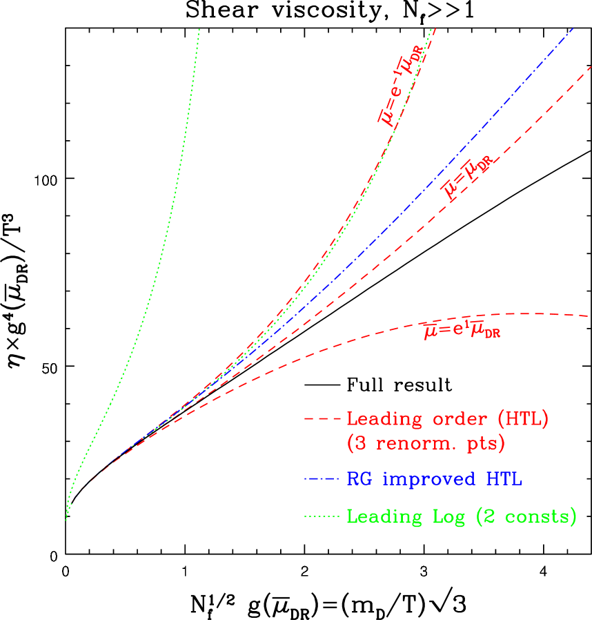
FIG. 7.: Shear viscosity computed with various approximations. The leading order calculation has an $O(g^{2}N_{\rm f})$ ambiguity associated with the renormalization point chosen for $g^{2}$; we show the result for three choices of renormalization point, $\bar{\mu}=\bar{\mu}_{\rm DR}$, and $e$ and $1/e$ times this, and “RG improved.” The leading log result is shown for two constants under the log. The curve which grossly disagrees with all others is using $O(1)=0$ in Eq. (46), the other leading-log curve picks the $O(1)$ constant to reproduce the leading order result at the smallest value of $g\sqrt{N_{\rm f}}$.

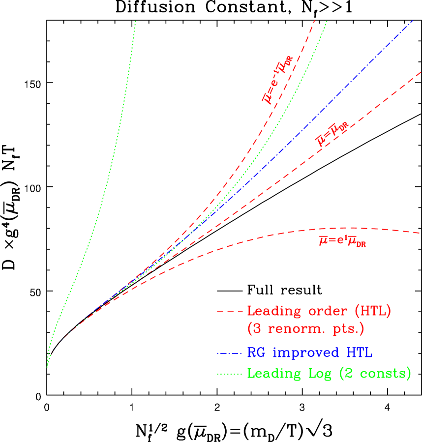
FIG. 8.: Same as Fig. 7 but for flavor diffusion.

There is a particularly natural choice for the renormalization point, which is the one for which tree expressions give the correct infrared, thermodynamic description of the gauge field physics. This is the “dimensional reduction” value $\bar{\mu}=\pi e^{-\gamma_{\rm E}}T$ [25]. We have chosen this as a “central” value for the presentation of results, and we illustrate the dependence on $\bar{\mu}$ by varying renormalization point by a factor of $e$ on either side.

An alternative approach is to settle the renormalization point dependence by including the real part of the (very simple) vacuum self-energy contribution everywhere, in addition to the HTL approximation of the thermal contribution. This is equivalent to using $g^{2}(\bar{\mu}=|\omega^{2}-q^{2}|)$ as the value of $g^{2}$ when the exchange momentum is $(\omega,q)$–that is, allowing the gauge coupling to run as the exchange momentum varies inside the integral in Eq. (31). We therefore term this a “renormalization group improved” leading order calculation. It is not correct beyond leading order in $g^{2}N_{\rm f}$, but it is free of renormalization point ambiguities. It is also shown in Figs. 7 and 8. The RG improved result systematically lies above the $\bar{\mu}=\bar{\mu}_{\rm DR}$ value, and turns out to be a worse approximation over the entire range considered. Note the strikingly good performance of the $\bar{\mu}=\bar{\mu}_{\rm DR}$ renormalization point, leading-order result, especially at small coupling. We interpret this as the result of “getting the renormalization point right”; the leading thermal correction, left out when we make the HTL approximation, cancels the vacuum running of the coupling and effectively sets $g^{2}\simeq g^{2}(\bar{\mu}_{\rm DR})$ in the soft exchange momentum region.

The figures also show the result of the leading-log calculation. There is an even more severe ambiguity in the leading-log calculation than in the leading order one; we do not know the $O(1)$ constant in Eq. (46). We display two values. The curve in each figure which lies above all other curves is setting $O(1)=0$ in Eq. (46), while the curve which tracks very closely the $\bar{\mu}=\bar{\mu}_{\rm DR}e^{-1}$ leading order curve is the result if we choose the $O(1)$ constant to match the leading order calculation at the smallest value of $m_{\rm D}/T$ shown. The ambiguity in the leading-log result is large even where the coupling is weak, and the naive choice $O(1)=0$ in Eq. (46) gives horrible results. However, what amounts to a “next to leading log” calculation works surprisingly well, comparably to leading order.

VI Conclusions

Computing transport coefficients, or any other quantity involving infrared limits of correlation functions, is a difficult problem in the context of relativistic gauge theories. We have shown that, in a rather special limit, this problem simplifies and the calculation, though still difficult, is tractable. This limit is the limit of a large number of fermions, $N_{\rm f}\gg 1$, expanding to leading nontrivial order in $1/N_{\rm f}$. In this limit, nonabelian effects become unimportant. Furthermore, the fermions enjoy nearly free dispersion relations, with corrections (both dispersion and scattering corrections) suppressed by $1/N_{\rm f}$. This allows a kinetic theory treatment of transport coefficients, which we have presented.

This kinetic treatment is actually simpler than a kinetic treatment of QED or QCD would be, if we intended to compute to leading order in $g$. In particular, in large $N_{\rm f}$ QED, there are no contributions at leading order from Compton scattering and annihilation to gauge bosons, or from interference diagrams or bremsstrahlung processes. Nonabelian effects are also irrelevant at leading order, so the QED and QCD calculations differ only by group factors. The structure of the scattering integral is simple enough that it is possible to carry the calculation out nonperturbatively in $g^{2}N_{\rm f}$, though this demands some care in the treatment of the scattering matrix element. In particular, the hard thermal loop (HTL) approximation for the thermal self-energy is inadequate, and a general expression for the thermal self-energy is needed.

It is also possible to perform a leading order in $g^{2}N_{\rm f}$ calculation by making the hard thermal loop (HTL) approximation. This permits an interesting test of the quality of the HTL approximation. Because the physics of this model is missing some complications present in QED and QCD (such as bremsstrahlung), we expect the HTL approximation to work, if anything, better in this model than in realistic QED or QCD. In fact, corrections to the HTL leading order calculation which we made here are parametrically $O(g^{2}N_{\rm f})$, while in full QED or QCD we believe that gauge boson emission processes and nonabelian effects (QCD only) will introduce $O(g)$ corrections.

Our results for the comparison between the complete solution and the HTL approximation are presented in Fig. 7 and Fig. 8, which constitute the main results of this paper. They show that, for $g^{2}N_{\rm f}\leq 1$, the leading order treatment is accurate to a few percent. This is good news for QED, where the coupling is indeed small. For instance, between the electron and muon mass scales, the QED coupling is $g\sqrt{N_{\rm f}}\simeq.30$. At this coupling the difference between the HTL and full treatments is less than $0.3\%$. Even at this coupling, however, a calculation to leading order in the logarithm of the coupling is of very little value.

On the other hand, as the coupling grows larger, the leading order treatment becomes much less reliable and more renormalization point dependent. In the theory we have looked at, the size of the renormalization point dependence of the leading order calculation and the size of its error (its difference from the exact result) are comparable. However, the “RG improved” calculation shows that the error is probably not due to a poor choice of renormalization point, but is a failure of the HTL approximation to correctly represent the thermal part of the self-energy. This is mixed news for QCD.

We can estimate how accurate a leading order calculation of transport coefficients in QCD would be by seeing how accurate the large $N_{\rm f}$ results are at a value of the Debye mass $m_{\rm D}/T$ equal to the relevant QCD value. First consider QCD for $T$ at the electroweak scale, $T\sim 100$GeV. Taking $\alpha_{\rm s}=0.11$, $N_{\rm f}=6$ and using Eq. (42), we find this corresponds to $g\sqrt{N_{\rm f}}\simeq 2.9$. For this value, the renormalization point uncertainty in the leading order value is about $30\%$. This is not so bad, though in full QCD the actual error will likely be larger than this.

The correction is much more severe at $T\sim$1GeV, where the coupling is much larger. This value of $T$ gives a $g$ roughly equal to the right hand edge of the figures, where the renormalization point sensitivity of the leading order calculation is at least a factor of 2. Therefore, at temperatures which may realistically be obtained in heavy ion collisions in the foreseeable future, a full leading order calculation is at best a factor of 2 estimate.

A Integration variables

Both $s$ and $t$ channel scattering processes must be computed in the main text. Different simplifications of the phase space integration in Eq. (31) prove most convenient for $s$ and $t$ channel scattering processes. It is convenient to have, as integration variables, the magnitudes of the spatial and temporal components of the momentum carried by the gauge boson, since it is by far easiest to express $|{\cal M}|^{2}$ in terms of these. Here we present both choices for phase space parameterization we have found useful. Note that we always take the external momenta to be strictly lightlike (massless dispersion relations), meaning $p_{0}=|{\bf p}|\equiv p$, which is justified at leading order in $1/N_{\rm f}$.

1 $t$ channel exchange

First consider the case were ${\bf p}^{\prime}-{\bf p}$ is the exchange momentum. Then in the collision integral , Eq. (31), it is convenient to use the spatial $\delta$ function to perform the ${\bf k}^{\prime}$ integration, and to shift the ${\bf p}^{\prime}$ integration into an integration over ${\bf p}^{\prime}{-}{\bf p}\equiv{\bf q}$. We may write the angular integrals in spherical coordinates with ${\bf q}$ as the $z$ axis and choose the $x$ axis so ${\bf p}$ lies in the $x$-$z$ plane. This yields

$$\beta^{3}\int\frac{d^{3}{\bf p}d^{3}{\bf k}d^{3}{\bf p}^{\prime}d^{3}{\bf k}^{\prime}}{(2\pi)^{12}16pkp^{\prime}k^{\prime}}(2\pi)^{4}\delta^{3}({\bf p}+{\bf k}-{\bf p}^{\prime}-{\bf k}^{\prime})\delta(p+k-p^{\prime}-k^{\prime})$$ (A1)

$$= \frac{\beta^{3}}{2^{9}\pi^{6}}\int_{0}^{\infty}\!\!\!q^{2}dq\>p^{2}dp\>k^{2}dk\int_{-1}^{1}\!\!d\cos\theta_{pq}\>d\cos\theta_{kq}\int_{0}^{2\pi}\!\!d\phi\frac{1}{p\,k\,p^{\prime}\,k^{\prime}}\delta(p{+}k{-}p^{\prime}{-}k^{\prime})\,,$$ (A2)

where $q=|{\bf q}|$, and $p^{\prime}$ and $k^{\prime}$ become dependent variables, $p^{\prime}\equiv|{\bf q}+{\bf p}|$ and $k^{\prime}\equiv|{\bf k}-{\bf q}|$. $\phi$ is the azimuthal angle of ${\bf k}$ (and ${\bf k}^{\prime}$) [i.e., the angle between the ${\bf p}$-${\bf q}$ plane and the ${\bf k}$-${\bf q}$ plane], and $\theta_{pq}$ is the plasma frame angle between ${\bf p}$ and ${\bf q}$, $\cos\theta_{pq}\equiv\hat{\bf p}\cdot\hat{\bf q}$, etc.

Following Baym et al. [13], it is convenient to introduce a dummy integration variable $\omega$, defined by a $\delta$ function to equal the energy transfer $p^{\prime}-p$, so that

$$\delta(p+k-p^{\prime}-k^{\prime})=\int_{-\infty}^{\infty}d\omega\>\delta(\omega+p-p^{\prime})\,\delta(\omega-k+k^{\prime})\,.$$ (A3)

Evaluating $p^{\prime}=|{\bf p}+{\bf q}|$ in terms of $p$, $q$, and $\cos\theta_{pq}$, and defining $t=\omega^{2}-q^{2}$ (which is the usual Mandelstam variable), one finds

$$\delta(\omega+p-p^{\prime}) = \frac{p^{\prime}}{pq}\>\delta\biggl{(}\cos\theta_{pq}-\frac{\omega}{q}-\frac{t}{2pq}\biggr{)}\Theta(\omega+p)\,,$$ (A4)

$$\delta(\omega-k+k^{\prime}) = \frac{k^{\prime}}{kq}\>\delta\biggl{(}\cos\theta_{kq}-\frac{\omega}{q}+\frac{t}{2kq}\biggr{)}\Theta(k-\omega)\,.$$ (A5)

Here $\Theta$ is the step function. The $\cos\theta$ integrals may now be trivially performed and yield 1 provided $p>{\textstyle{1\over 2}}(q-\omega)$, $k>{\textstyle{1\over 2}}(q+\omega)$, and $|\omega|<q$; otherwise the argument of a $\delta$ function has no zero for any $|\cos\theta|\leq 1$. The integration range becomes

$$\frac{\beta^{3}}{2^{9}\pi^{6}}\int_{0}^{\infty}\!\!dq\int_{-q}^{q}\!d\omega\int_{\frac{q-\omega}{2}}^{\infty}dp\int_{\frac{q+\omega}{2}}^{\infty}dk\int_{0}^{2\pi}\!\!d\phi\,,$$ (A6)

with $p^{\prime}=p{+}\omega$, $k^{\prime}=k{-}\omega$. For evaluating the final factor of Eq. (31), note that

$$I_{i\cdots j}(\hat{\bf p})\,I_{i\cdots j}(\hat{\bf k})=P_{\ell}(\cos\theta_{pk})\,,$$ (A7)

where $P_{\ell}$ is the $\ell$’th Legendre polynomial, and $\ell=1$ if there is one index (diffusion) and $\ell=2$ if there are two indices (shear viscosity). We will therefore need expressions for the angles between all species, as well as the remaining Mandelstam variables $s$ and $u$, which may appear in ${\cal M}^{2}$. They are

$$s = \frac{-t}{2q^{2}}\left\{\left[(p+p^{\prime})(k+k^{\prime})+q^{2}\right]-\cos\phi\>\sqrt{\textstyle\left(4pp^{\prime}+t\right)\left(4kk^{\prime}+t\right)}\,\right\}\,,$$ (A8)

$$u = -t-s\,,$$ (A9)

and

$$\cos\theta_{pq}\> = \frac{\omega}{q}+\frac{t}{2pq}\,,\hskip 77.32942pt\;\cos\theta_{p^{\prime}q}\>=\frac{\omega}{q}-\frac{t}{2p^{\prime}q}\,,$$ (A10)

$$\cos\theta_{kq}\> = \frac{\omega}{q}-\frac{t}{2kq}\,,\hskip 79.49744pt\cos\theta_{k^{\prime}q}\>=\frac{\omega}{q}+\frac{t}{2k^{\prime}q}\,,$$ (A11)

$$\cos\theta_{pp^{\prime}} = 1+\frac{t}{2pp^{\prime}}\,,\hskip 80.94205pt\cos\theta_{kk^{\prime}}\>=1+\frac{t}{2kk^{\prime}}\,,$$ (A12)

$$\cos\theta_{pk^{\prime}} = 1+\frac{u}{2pk^{\prime}}\,,\hskip 80.58144pt\cos\theta_{p^{\prime}k}\>=1+\frac{u}{2p^{\prime}k}\,,$$ (A13)

$$\cos\theta_{pk}\> = 1-\frac{s}{2pk}\,,\hskip 83.11005pt\cos\theta_{p^{\prime}k^{\prime}}=1-\frac{s}{2p^{\prime}k^{\prime}}\,.$$ (A14)

The $\phi$ integration can be done analytically in all cases in this paper, but the other integrals cannot.

2 $s$ channel exchange

When the exchange gauge boson carries momentum ${\bf p}+{\bf k}$, it is convenient to use a different parameterization of phase space. Again the spatial $\delta$ function in Eq. (31) is used to perform the ${\bf k}^{\prime}$ integration, but now the $k$ integration is shifted to an integral over ${\bf q}\equiv{\bf p}+{\bf k}$, the total incoming spatial momentum. Again we use spherical coordinates, with ${\bf q}$ on the $z$ axis and ${\bf p}$ in the $x$-$z$ plane. In these variables, the integration measure becomes

$$\beta^{3}\int\frac{d^{3}{\bf p}d^{3}{\bf k}d^{3}{\bf p}^{\prime}d^{3}{\bf k}^{\prime}}{(2\pi)^{12}16pkp^{\prime}k^{\prime}}(2\pi)^{4}\delta^{3}({\bf p}+{\bf k}-{\bf p}^{\prime}-{\bf k}^{\prime})\delta(p+k-p^{\prime}-k^{\prime})$$ (A15)

$$= \frac{\beta^{3}}{2^{9}\pi^{6}}\int_{0}^{\infty}\!\!\!q^{2}dq\>p^{2}dp\>{p^{\prime}}^{2}dp^{\prime}\int_{-1}^{1}\!\!d\cos\theta_{pq}\>d\cos\theta_{p^{\prime}q}\int_{0}^{2\pi}\!\!d\phi\frac{1}{p\,k\,p^{\prime}\,k^{\prime}}\>\delta(p{+}k{-}p^{\prime}{-}k^{\prime})\,,$$ (A16)

where $k=|{\bf q}{-}{\bf p}|$ and $k^{\prime}=|{\bf q}{-}{\bf p}^{\prime}|$, and $\phi$ is the azimuthal angle of ${\bf p}^{\prime}$, meaning the angle between the ${\bf q},{\bf p}$ plane and the ${\bf q},{\bf p}^{\prime}$ plane.

Next, we re-write the energy delta function in terms of $\omega$, the total energy;

$$\delta(p+k-p^{\prime}-k^{\prime})=\int_{0}^{\infty}d\omega\>\delta(\omega-p-k)\,\delta(\omega-p^{\prime}-k^{\prime})\,.$$ (A17)

In terms of the remaining integration variables, and defining $s=\omega^{2}-q^{2}$ (which again is the Mandelstam variable), one finds

$$\delta(\omega-p-k) = \frac{k}{pq}\>\,\delta\left(\cos\theta_{pq}\>-\frac{\omega}{q}+\frac{s}{2pq}\>\right)\Theta(\omega-p\>)\,,$$ (A18)

$$\delta(\omega-p^{\prime}-k^{\prime}) = \frac{k^{\prime}}{p^{\prime}q}\,\delta\left(\cos\theta_{p^{\prime}q}-\frac{\omega}{q}+\frac{s}{2p^{\prime}q}\right)\Theta(\omega-p^{\prime})\,,$$ (A19)

which performs the integrals over $\cos\theta_{pq}$ and $\cos\theta_{p^{\prime}q}$. There is only a solution provided $q<\omega$, $|2p-\omega|<q$, and $|2p^{\prime}-\omega|<q$. The integration measure becomes

$$\frac{\beta^{3}}{2^{9}\pi^{6}}\int_{0}^{\infty}\!\!d\omega\int_{0}^{\omega}\!dq\int_{\omega-q\over 2}^{\omega+q\over 2}\!\!dp\int_{\omega-q\over 2}^{\omega+q\over 2}\!\!dp^{\prime}\int_{0}^{2\pi}\!\!d\phi\,,$$ (A20)

with $k=\omega{-}p$, $k^{\prime}=\omega{-}p^{\prime}$. The Mandelstam variables are

$$t = \frac{s}{2q^{2}}\left\{\left[(p-k)(p^{\prime}-k^{\prime})-q^{2}\right]+\cos\phi\sqrt{(4pk-s)(4p^{\prime}k^{\prime}-s)}\right\}\,,$$ (A21)

$$u = -s-t\,.$$ (A22)

The angles with respect to ${\bf q}$ are

$$\cos\theta_{pq} = \frac{\omega}{q}-\frac{s}{2pq}\,,\hskip 78.05173pt\cos\theta_{p^{\prime}q}=\frac{\omega}{q}-\frac{s}{2p^{\prime}q}\,,$$ (A23)

$$\cos\theta_{kq} = \frac{\omega}{q}-\frac{s}{2kq}\,,\hskip 78.05173pt\cos\theta_{k^{\prime}q}=\frac{\omega}{q}-\frac{s}{2k^{\prime}q}\,,$$ (A24)

and the remaining angles are as in Eq. (A14).

Again the $\phi$ integral can be performed analytically, but the other integrals cannot.

B Matrix elements

In this appendix we present the matrix elements for $s$ and $t$ channel gauge boson exchange. These must be calculated without making any expansion in $q\ll p$ or in small self-energy; for our purpose the self-energy must be taken to be an $O(1)$ correction and all momenta must be considered to be the same order.

The quantity “[$t^{2}+u^{2}$$/s^{2}$]”, introduced as a shorthand in Eq. (32), technically means

$$\frac{1}{8}D^{\rm ret}_{\mu\alpha}D^{\rm adv}_{\nu\beta}{\rm Tr}(\not{\!p\,}\gamma^{\mu}\not{\!k\,}\gamma^{\nu}){\rm Tr}(\not{\!p\,}^{\prime}\gamma^{\alpha}\not{\!k\,}^{\prime}\gamma^{\beta})\,.$$ (B1)

Following the previous appendix we denote the plasma frame frequency and momentum carried by the gauge boson propagator as $\omega$ and $q$. The retarded gauge boson propagator $D^{\rm ret}_{\mu\nu}$ is most conveniently expressed in Coulomb gauge–the result for Eq. (B1) being gauge invariant:

$$D^{\rm ret}_{00}(\omega,{\bf q}) = \frac{1}{q^{2}-\Pi_{\rm L}^{\rm ret}(\omega,q)}\,,$$ (B2)

$$D^{\rm ret}_{ij}(\omega,{\bf q}) = \frac{\delta_{ij}-\hat{\bf q}_{i}\hat{\bf q}_{j}}{q^{2}-\omega^{2}+\Pi_{\rm T}^{\rm ret}(\omega,q)}\,,$$ (B3)

$$D^{\rm ret}_{0i}(\omega,{\bf q}) = D_{i0}(\omega,{\bf q})\>=\>0\,.$$ (B4)

The sign of $D^{\rm ret}_{ij}$ is opposite the most common convention because we use a $({-}{+}{+}{+})$ metric; but we have chosen the sign of $\Pi_{\rm T}$ to correspond to common usage. The advanced propagator is given by complex conjugating these expressions. In what follows we drop the [ret] superscript from the self-energies.

It will be convenient for our purposes to define nonstandard normalization self-energies

$$\tilde{\Pi}_{\rm L}\equiv-\Pi_{\rm L}\,,\qquad\tilde{\Pi}_{\rm T}\equiv\frac{q^{2}}{q^{2}-\omega^{2}}\Pi_{\rm T}\,.$$ (B6)

In terms of these, evaluating Eq. (B1) gives

$$2\;\raisebox{8.00003pt}{\mbox{``}}\!\!\left(\frac{t^{2}+u^{2}}{s^{2}}\right)\!\!\raisebox{8.00003pt}{\mbox{''}}\> = \frac{1}{|q^{2}+\tilde{\Pi}_{\rm L}|^{2}}(4pk{-}s)(4p^{\prime}k^{\prime}{-}s)$$ (B9)

$$+\frac{2}{\left|(q^{2}+\tilde{\Pi}_{\rm L}^{*})(q^{2}+\tilde{\Pi}_{\rm T})\right|}(p{-}k)(p^{\prime}{-}k^{\prime})\sqrt{(4pk{-}s)(4p^{\prime}k^{\prime}{-}s)}\,\cos\phi$$

$$+\frac{1}{|q^{2}+\tilde{\Pi}_{\rm T}|^{2}}\left((4pk{-}s)(4p^{\prime}k^{\prime}{-}s)\,\cos^{2}\phi+q^{2}(2\omega^{2}-4pk-4p^{\prime}k^{\prime})\right)\,.$$

The analogous result for $t$ channel exchange is

$$2\;\raisebox{8.00003pt}{\mbox{``}}\!\!\left(\frac{s^{2}+u^{2}}{t^{2}}\right)\!\!\raisebox{8.00003pt}{\mbox{''}}\> = \frac{1}{|q^{2}+\tilde{\Pi}_{\rm L}|^{2}}(4pp^{\prime}{+}t)(4kk^{\prime}{+}t)$$ (B12)

$$-\frac{2}{\left|(q^{2}+\tilde{\Pi}_{\rm L}^{*})(q^{2}+\tilde{\Pi}_{\rm T})\right|}(p{+}p^{\prime})(k{+}k^{\prime})\sqrt{(4pp^{\prime}{+}t)(4kk^{\prime}{+}t)}\,\cos\phi$$

$$+\frac{1}{|q^{2}+\tilde{\Pi}_{\rm T}|^{2}}\left((4pp^{\prime}{+}t)(4kk^{\prime}{+}t)\,\cos^{2}\phi+q^{2}(2\omega^{2}+4pp^{\prime}+4kk^{\prime})\right)\,.$$

The variables in these expressions, such as $\phi$, $s$, $t$, $p$, etc are defined in Appendix A. In particular the definition of $\phi$ in Eq. (B9) is the angle between the ${\bf q},{\bf p}$ plane and the ${\bf q},{\bf p}^{\prime}$ plane, whereas in Eq. (B12) it is the angle between the ${\bf q},{\bf p}$ and ${\bf q},{\bf k}$ planes.

Complete expressions for $\Pi_{\rm L}$ and $\Pi_{\rm T}$ were obtained by Weldon [27], and the usual expressions for the hard thermal loop limit of the self-energies were extracted as a particular limit. The vacuum parts are simple:

$$\tilde{\Pi}_{\rm T,\;vac}=\tilde{\Pi}_{\rm L,\;vac}=\frac{g^{2}N_{\rm f}}{12\pi^{2}}q^{2}\left[-\log\left(\frac{|\omega^{2}-q^{2}|}{\bar{\mu}^{2}}\right)+\frac{5}{3}+i\pi\Theta(\omega^{2}-q^{2})\right]\,.$$ (B13)

The imaginary part exists for timelike momenta and represents the vacuum rate of decay into a fermion pair. The full self-energy is the sum of a vacuum and a thermal part. The thermal parts of the self-energies are

$$\tilde{\Pi}_{\rm L,\;th}=\frac{g^{2}N_{\rm f}T^{2}}{3}H(\omega,q)\,,\qquad\tilde{\Pi}_{\rm T,\;th}=\frac{g^{2}N_{\rm f}T^{2}}{3}\left(-\frac{1}{2}H(\omega,q)+\frac{q^{2}}{2(q^{2}-\omega^{2})}G(\omega,q)\right)\,,$$ (B14)

where $H(\omega,q)$ and $G(\omega,q)$ are, using the shorthand $2\omega_{+}\equiv\omega{+}q$ and $2\omega_{-}\equiv\omega{-}q$,

$${\rm Re}\>G(\omega,q) = \frac{3}{\pi^{2}T^{2}}\int_{0}^{\infty}\!\!\!dk\>f_{0}(k)\left(4k+\frac{q^{2}{-}\omega^{2}}{2q}\ln\left[\frac{(k{+}\omega_{-})(k{-}\omega_{+})}{(k{+}\omega_{+})(k{-}\omega_{-})}\right]\right)\,,$$ (B15)

$${\rm Re}\>H(\omega,q) = \frac{3}{\pi^{2}T^{2}}\int_{0}^{\infty}\!\!\!dk\>f_{0}(k)\Bigg{(}2k-\frac{4k^{2}{+}\omega^{2}{-}q^{2}}{4q}\ln\left[\frac{(k{+}\omega_{-})(k{-}\omega_{+})}{(k{+}\omega_{+})(k{-}\omega_{-})}\right]$$ (B17)

$$\qquad\qquad-\frac{2k\omega}{q}\ln\frac{\omega_{+}}{\omega_{-}}-\frac{k\omega}{q}\ln\left[\frac{(k{+}\omega_{-})(k{-}\omega_{-})}{(k{+}\omega_{+})(k{-}\omega_{+})}\right]\Bigg{)}\,,$$

$${\rm Im}\>G(\omega,q) = \frac{3}{\pi T^{2}}\int_{0}^{\infty}\!\!\!dk\>f_{0}(k)\frac{q^{2}{-}\omega^{2}}{2q}\Big{[}\Theta(k{+}\omega_{+})\Theta(-k{-}\omega_{-})-\Theta(-k{+}\omega_{+})\Theta(k{-}\omega_{-})\Big{]}\,,$$ (B18)

$${\rm Im}\>H(\omega,q) = \frac{3}{\pi T^{2}}\int_{0}^{\infty}\!\!\!dk\>f_{0}(k)\Bigg{[}-\frac{(2k{+}\omega)^{2}-q^{2}}{4q}\Theta(k{+}\omega_{+})\Theta(-k{-}\omega_{-})$$ (B21)

$$\hskip 98.28723pt+\frac{(2k{-}\omega)^{2}-q^{2}}{4q}\ \Theta(k{-}\omega_{-})\Theta(-k{+}\omega_{+})$$

$$\hskip 98.28723pt+\frac{2k\omega}{q}\Theta(\omega_{+})\Theta(-\omega_{-})\Bigg{]}\,.$$

The hard thermal loop limit means taking $\omega\ll T$, $q\ll T$, and extracting the nonvanishing part. The values of these integrals, in this limit, depend only on $\omega/q$ and are

$$H_{\rm HTL}(\omega/q) = 1-\frac{\omega}{2q}\ln\frac{\omega_{+}}{\omega_{-}}+i\frac{\pi\omega}{2q}\Theta(\omega_{+})\Theta(-\omega_{-})\,,$$ (B22)

$$G_{\rm HTL}(\omega/q) = 1\,.$$ (B23)

However at general $\omega/T$, $q/T$, only a few of the integrals can be performed analytically and some have to be done numerically. However, all required integrals can be done quickly and to high precision by numerical quadratures integration, and their evaluation does not limit either the accuracy or speed of any subsequent integrations.

Note that, for timelike momenta, the thermal contributions to the imaginary parts of the self-energies are of opposite sign as the vacuum parts, and represent Pauli blocking of pair production. The thermal contribution to the imaginary part at spacelike momenta, absent in the vacuum theory, represents Landau damping. In the HTL limit only the imaginary part arising from $\Theta(\omega_{+})\Theta(-\omega_{-})$ contributes. All real parts are even in $\omega$ and all imaginary parts are odd in $\omega$.

REFERENCES

- [1] L. V. Keldysh, Zh. Eksp. Teor. Fiz. 47, 1515 (1964).
- [2] E. Braaten and R. D. Pisarski, Nucl. Phys. B337 (1990) 569; J. Frenkel and J. Taylor, Nucl. Phys. B334, 199 (1990); J. Taylor and S. Wong, Nucl. Phys. B346, 115 (1990).
- [3] E. Braaten and R. D. Pisarski, Phys. Rev. D 42, 2156 (1990); E. Braaten and R. D. Pisarski, Phys. Rev. D 46, 1829 (1992); T. S. Biro and M. H. Thoma, Phys. Rev. D 54, 3465 (1996) [hep-ph/9603339];
- [4] E. Braaten and M. H. Thoma, Phys. Rev. D 44, 1298 (1991).
- [5] D. Bodeker, Phys. Lett. B 426, 351 (1998) [hep-ph/9801430]; Nucl. Phys. B 566, 402 (2000) [hep-ph/9903478]; Nucl. Phys. B 559, 502 (1999) [hep-ph/9905239].
- [6] S. Jeon, Phys. Rev. D52, 3591 (1995) [hep-ph/9409250].
- [7] A. Hosoya and K. Kajantie, Nucl. Phys. B250, 666 (1985).
- [8] A. Hosoya, M. Sakagami and M. Takao, Annals Phys. 154, 229 (1984).
- [9] S. Chakrabarty, Pramana 25, 673 (1985).
- [10] W. Czyż and W. Florkowski, Acta Phys. Polon. B17, 819 (1986).
- [11] D. W. von Oertzen, Phys. Lett. B280, 103 (1992).
- [12] M. H. Thoma, Phys. Lett. B269, 144 (1991).
- [13] G. Baym, H. Monien, C. J. Pethick and D. G. Ravenhall, Phys. Rev. Lett. 64, 1867 (1990); Nucl. Phys. A525, 415C (1991).
- [14] H. Heiselberg, Phys. Rev. D49, 4739 (1994) [hep-ph/9401309].
- [15] H. Heiselberg, Phys. Rev. Lett. 72, 3013 (1994) [hep-ph/9401317].
- [16] G. Baym and H. Heiselberg, Phys. Rev. D56, 5254 (1997) [astro-ph/9704214].
- [17] M. Joyce, T. Prokopec and N. Turok, Phys. Rev. D53, 2930 (1996) [hep-ph/9410281].
- [18] G. D. Moore and T. Prokopec, Phys. Rev. D52, 7182 (1995) [hep-ph/9506475].
- [19] M. Joyce, T. Prokopec and N. Turok, Phys. Rev. D53, 2958 (1996) [hep-ph/9410282].
- [20] P. Arnold, G. D. Moore and L. G. Yaffe, JHEP0011, 001 (2000) [hep-ph/0010177].
- [21] E. Braaten and A. Nieto, Phys. Rev. D 53, 3421 (1996) [hep-ph/9510408].
- [22] L. P. Kadanoff and G. Baym, “Quantum Statistical Mechanics,” Benjamin, New York (1962).
- [23] E. Calzetta and B. L. Hu, Phys. Rev. D37, 2878 (1988); E. A. Calzetta, B. L. Hu and S. A. Ramsey, Phys. Rev. D61, 125013 (2000) [hep-ph/9910334].
- [24] S. R. De Groot, W. A. Van Leeuwen and C. G. Van Weert, “Relativistic Kinetic Theory. Principles And Applications,” Amsterdam, Netherlands: North-holland ( 1980) 417p.
- [25] K. Kajantie, M. Laine, K. Rummukainen and M. Shaposhnikov, Nucl. Phys. B 458, 90 (1996) [hep-ph/9508379].
- [26] P. Aurenche, F. Gelis, R. Kobes and H. Zaraket, Phys. Rev. D 60, 076002 (1999) [hep-ph/9903307]; P. Aurenche, F. Gelis and H. Zaraket, Phys. Rev. D 61, 116001 (2000) [hep-ph/9911367]; P. Aurenche, F. Gelis and H. Zaraket, Phys. Rev. D 62, 096012 (2000) [hep-ph/0003326].
- [27] H. A. Weldon, Phys. Rev. D26, 1394 (1982).