Lepton Flavor Violating $Z$ Decays in the Zee Model

Abstract

We calculate lepton flavor violating (LFV) $Z$ decays $Z\rightarrow{{e_{i}^{\pm}}}e_{j}^{\mp}$ ($i,j=e,\mu,\tau$ ; $i\neq j$) in the Zee model keeping in view the radiative leptonic decays $e_{i}\rightarrow e_{j}\gamma$ ( $i=\mu$, $\tau$ ; $j=e$, $\mu$ ; $i\neq j$ ), $\mu$ decay and anomalous muon magnetic moment ($\mu$AMM). We investigate three different cases of Zee $f_{ij}$ coupling (A) $f_{e\mu}^{2}$ = $f_{\mu\tau}^{2}$ = $f_{\tau e}^{2}$, (B) $f_{e\mu}^{2}$ $\gg$ $f_{\tau e}^{2}$ $\gg$ $f_{\mu\tau}^{2}$, and (C) $f_{\mu\tau}^{2}$ $\gg$ $f_{e\mu}^{2}$ $\gg$ $f_{\tau e}^{2}$ subject to the neutrino phenomenology. Interestingly, we find that, although the case (C) satisfies the large excess value of $\mu$AMM, however, it is unable to explain the solar neutrino experimental result, whereas the case (B) satisfies the bi-maximal neutrino mixing scenario, but confronts with the result of $\mu$AMM experiment. We also find that among all the three cases, only the case (C) gives rise to largest contribution to the ratio $B(Z\rightarrow e^{\pm}\tau^{\mp})$/$B(Z\rightarrow\mu^{\pm}\mu^{\mp})$ $\simeq$ ${10}^{-8}$ which is still two order less than the accessible value to be probed by the future linear colliders, whereas for the other two cases, this ratio is too low to be observed even in the near future for all possible LFV $Z$ decay modes.

I Introduction

The high statistics results of the SuperKamiokande (SK) atmospheric neutrino experiment [1] and the solar neutrino experiment [2] have strengthen the conjecture of neutrino flavor oscillation from one species to another. The phenomena of neutrino oscillation leads to non-zero neutrino mass and the scale of which is $\sim$ eV predominantly set by the atmospheric and solar neutrino experimental results. Such a tiny neutrino mass could be generated by several ways, namely, see-saw mechanism [3], non-renormalizable operators [4] or through the radiative ways at the one or two loop level. One of the most well known model of radiative neutrino mass generation is proposed by Zee [5] in which small neutrino mass is generated at the one loop level due to charged scalar exchange through explicit lepton number violation. The model has been investigated by many authors [6 - 11]. The model contains one extra charged singlet scalar field with non-zero lepton number and another doublet Higgs field in addition with the standard model (SM) contents. The scalar field content of the Zee model is not only responsible to generate tiny neutrino masses but also gives rise to non-standard interactions due to the presence of charged scalar fields, e.g., one of them is the anomalous muon magnetic moment ($\mu$AMM). The excess value of ($\mu$AMM), $\delta a_{\mu}$ = (43$\pm$ 16)$\times$ ${10}^{-10}$ recently reported by E821 Collaboration [12] leads to the new source of interactions beyond the SM level. Furthermore, the Zee model leads to possible Lepton Flavor Violating (LFV) $Z$ decays [13], such as, $Z\rightarrow{e_{i}^{\pm}}e_{j}^{\mp}$ ($\it{i,\,j}=e$, $\mu$, $\tau$ and hereafter, we will assume $i\neq j$ unless otherwise stated ), which have taken interest in view of future collider plans. The present sensitivity of the measurement of branching ratio of $Z\rightarrow$ $e_{i}^{\pm}e_{j}^{\mp}$ at LEP is $\sim$ ${10}^{-5}$ whereas future linear colliders (NLC, JLC, Tesla GigaZ) will bring it down to $\sim$ ${10}^{-8}$ and thus the testability of such model will be increased due to higher sensitivity of measurement which could be able to reveal new physics beyond the SM.

In the present work, we calculate $\mu$AMM and LFV $Z$ decays in the Zee model keeping in view the other constraints arising due to $\mu$ decay and other LFV radiative lepton decays. We estimate $\mu$AMM and LFV $Z$ decays by utilizing the constraints on the parameter space obtained from the $\mu\rightarrow e{{\overline{\nu}}_{e}}\nu_{\mu}$ decay and also from radiative $e_{i}\rightarrow e_{j}\gamma$ ( $\it{i}$ = $\mu$, $\tau$ ; $\it{j}$ = $e,\mu$ ; $\it{i\neq j}$ ) decays. Recent works in this path have been done [14] in which the Zee model have been investigated in view of recent $\mu$AMM experimental result and LFV decays. In the present work, we restrict ourselves within the configuration of the minimal Zee model and we, particularly, investigate different hierarchical cases of Zee $f_{ij}$ coupling subject to the present neutrino phenomenology. The plan of the paper is as follows: In Section II, we will first briefly review the Zee model, its basic interaction Lagrangian, the charged scalar mixing and the neutrino mass matrix. The constraints on the Zee $f_{ij}$ coupling due to $\mu\rightarrow e{{\overline{\nu}}_{e}}\nu_{\mu}$ , $e_{i}\rightarrow e_{j}\gamma$ decays and $\mu$AMM are discussed in Section III. The LFV $Z$ decays are calculated in Section IV and Section V contains summary of the present work.

II Brief Review of the Zee Model

A The interaction Lagrangian

The interaction Lagrangian of the Zee model is given by

$${\cal L}=\sum_{i,j}f_{ij}\overline{\ell}_{iL}i\tau_{2}\ell^{c}_{jL}h^{-}+c_{12}\phi_{1}^{T}i\tau_{2}\phi_{2}h^{-}+\sum_{i}y_{i}\overline{\ell}_{iL}\phi_{2}e_{iR}+h.c.,$$

where we have dropped the quark interaction terms, and lepton number conserving Higgs potential terms. The lepton doublets are denoted as $\ell_{iL}$ ($i=1,2,3$) with the definition $\ell^{c}_{iL}=(\ell_{iL})^{c}=C\overline{\ell}_{iL}^{T}$ and $\phi_{a}$ ($a$ = 1, 2) are the Higgs doublets and $h^{-}$ is a charged singlet scalar field. The $f_{ij}$ terms can explicitly be written as follows:

  

$$\sum_{i,j}f_{ij}\overline{\ell}_{iL}i\tau_{2}\ell_{jL}^{c}h^{-}+h.c.=\sum_{i,j}f_{ij}(\overline{\nu}_{iL}e_{jL}^{c}-\overline{e}_{iL}\nu_{jL}^{c})h^{-}+h.c.$$

$$=2[f_{e\mu}(\overline{\nu}_{eL}\mu_{L}^{c}-\overline{e}_{L}\nu_{{\mu}L}^{c})+f_{\mu\tau}(\overline{\nu}_{{\mu}L}\tau_{L}^{c}-\overline{\mu}_{L}\nu_{{\tau}L}^{c})+f_{{\tau}e}(\overline{\nu}_{\tau L}e_{L}^{c}-\overline{\tau}_{L}\nu_{eL}^{c})]h^{-}+h.c.\,.$$

  

Since $\overline{e}_{iL}\nu_{jL}^{c}=\overline{\nu}_{jL}e_{iL}^{c}$, we can also re-express (2.2) as

  

$$2[f_{e\mu}(\overline{\mu}_{L}\nu_{eL}^{c}-\overline{e}_{L}\nu_{{\mu}L}^{c})+f_{\mu\tau}(\overline{\tau_{L}}\nu_{{\mu}L}^{c}-\overline{\mu}_{L}\nu_{{\tau}L}^{c})+f_{{\tau}e}(\overline{e}_{L}\nu_{{\tau}L}^{c}-\overline{\tau}_{L}\nu_{eL}^{c})]h^{-}+h.c.\ .$$

  

The $c_{12}$ term can explicitly be expressed as follows:

$$c_{12}\phi_{1}^{T}i\tau_{2}\phi_{2}h^{-}+h.c.=c_{12}(\phi^{+}_{1}\phi^{0}_{2}-\phi_{1}^{0}\phi_{2}^{+})h^{-}+h.c.$$

We define

$$\phi^{0}_{a}={\frac{1}{\sqrt{2}}}(v_{a}+H_{a}^{0}-i\chi_{a}^{0})\ ,$$

$$\chi^{0}=\chi^{0}_{1}\cos\beta-\chi^{0}_{2}\sin\beta\ ,\ \ \ \widetilde{\chi}^{0}=\chi_{1}^{0}\sin\beta+\chi_{2}^{0}\cos\beta\ ,$$

$$H^{0}=H_{1}^{0}\cos\beta-H^{0}_{2}\sin\beta\ ,\ \ \ \widetilde{H}^{0}=H_{1}^{0}\sin\beta+H_{2}^{0}\cos\beta\ ,$$

$$\phi^{+}=\phi_{1}^{+}\cos\beta-\phi_{2}^{+}\sin\beta\ ,\ \ \ \widetilde{\phi}^{+}=\phi^{+}_{1}\sin\beta+\phi_{2}^{+}\cos\beta\ ,$$

$$\tan\beta=v_{1}/v_{2}\ ,$$

where $v_{a}$ are the vacuum expectation values (VEV’s) of $\phi_{a}^{0}$, $\langle\phi^{0}_{a}\rangle=v_{a}/{\sqrt{2}}$.

By using the expressions (2.6)-(2.9), the $c_{12}$ term is expressed as follows:

$$c_{12}(\phi_{1}^{+}\phi_{2}^{0}-\phi_{2}^{+}\phi_{1}^{0})h^{-}+h.c.$$

$$={\frac{1}{\sqrt{2}}}c_{12}[\phi^{+}(\widetilde{v}+\widetilde{H}^{0}-i\widetilde{\chi}^{0})-\widetilde{\phi}^{+}(v+H^{0}-i\chi^{0})]h^{-}+h.c.,$$

where

$$v=v_{1}\cos\beta-v_{2}\sin\beta=0,$$

$$\widetilde{v}=v_{1}\sin\beta+v_{2}\cos\beta={\sqrt{v_{1}^{2}+v_{2}^{2}}}$$

$$=\frac{2M_{W}}{g}={\sqrt{2}}\times 174{\rm GeV}.$$

The components $\widetilde{\phi}^{+}$ and $\widetilde{\chi}^{0}$ are absorbed into the gauge bosons $W^{+}$ and $Z^{0}$, so that they are not physical particles. Therefore, the physical part in the $c_{12}$ term is only

$${\frac{1}{\sqrt{2}}}c_{12}\widetilde{v}\phi^{+}h^{-}+{\frac{1}{\sqrt{2}}}c_{12}\phi^{+}\widetilde{H}^{0}h^{-}+h.c..$$

The first term of Eq.(2.13) is a quadratic interaction term which induces the $\phi^{+}$-$h^{+}$ mixing as we show in the later part of this section. The second term is not relevant for our analysis.

The third term in the Lagrangian (2.1) is the conventional Yukawa coupling term :

$$\sum_{i}y_{i}(\overline{\nu}_{iL}\ \overline{e}_{iL})\left(\begin{array}[]{c}\phi^{+}_{2}\\ \phi^{0}_{2}\end{array}\right)e_{iR}=\sum_{i}y_{i}(\overline{\nu}_{iL}\phi^{+}_{2}+\overline{e}_{iL}\phi^{0}_{2})e_{iR}$$

$$={\frac{1}{\sqrt{2}}}\widetilde{v}\cos\beta\sum_{i}y_{i}(\overline{e}_{iL}e_{iR})-\sin\beta\sum_{i}y_{i}(\overline{\nu}_{iL}e_{iR})\phi^{+}$$

$$-{\frac{1}{\sqrt{2}}}\sum_{i}y_{i}(\overline{e}_{iL}e_{iR})[\sin\beta(H^{0}-i\chi^{0})-\cos\beta\widetilde{H}^{0}]$$

$$+({\rm unphysical}\ {\rm terms}),$$

so that the charged lepton masses $m_{ei}$ are given by

$$m_{ei}={\frac{1}{\sqrt{2}}}y_{i}{\widetilde{v}}\cos\beta.$$

The term $\sum_{i}y_{i}\sin\beta(\overline{\nu}_{iL}e_{iR})\phi^{+}$ together with the terms given in Eqs.(2.3) and (2.13) will contribute to the neutrino mass generation.

B The charged scalar boson mixing

The mass matrix for $(h^{+},\phi^{+})$ is given by

$$M^{2}=\left(\begin{array}[]{cc}M_{h}^{2}&c_{12}{{\widetilde{v}}/{\sqrt{2}}}\\ c_{12}{{\widetilde{v}}/{\sqrt{2}}}&M_{\phi}^{2}\end{array}\right)$$

where $M_{h}^{2}$ and $M_{\phi}^{2}$ are the coefficients of the $h^{+}h^{-}$, $\phi^{+}\phi^{-}$ terms of the scalar potential. We define an orthogonal transformation between the $h^{+}$ and $\phi^{+}$ scalar fields as

$$\left(\begin{array}[]{c}h^{+}\\ \phi^{+}\end{array}\right)=\left(\begin{array}[]{cc}\cos\theta&\sin\theta\\ -\sin\theta&\cos\theta\end{array}\right)\left(\begin{array}[]{c}H_{1}^{+}\\ H_{2}^{+}\end{array}\right),$$

by which we obtain

$$\left(\begin{array}[]{cc}h^{+}&\phi^{+}\end{array}\right)\left(\begin{array}[]{cc}M_{h}^{2}&c_{12}{{\widetilde{v}}/{\sqrt{2}}}\\ c_{12}{{\widetilde{v}}/{\sqrt{2}}}&M_{\phi}^{2}\end{array}\right)\left(\begin{array}[]{c}h^{-}\\ \phi^{-}\end{array}\right)$$

$$=\left(\begin{array}[]{cc}H^{+}_{1}&H_{2}^{+}\end{array}\right)\left(\begin{array}[]{cc}M_{1}^{2}&M_{12}\\ M_{12}&M_{2}^{2}\end{array}\right)\left(\begin{array}[]{c}H_{1}^{-}\\ H_{2}^{-}\end{array}\right),$$

$$M_{1}^{2}={\frac{M_{h}^{2}+M_{\phi}^{2}}{2}}+{\frac{M_{h}^{2}-M_{\phi}^{2}}{2}}\cos 2\theta-c_{12}{\frac{\widetilde{v}}{\sqrt{2}}}\sin 2\theta,$$

$$M_{2}^{2}={\frac{M_{h}^{2}+M_{\phi}^{2}}{2}}-{\frac{M_{h}^{2}-M_{\phi}^{2}}{2}}\cos 2\theta+c_{12}{\frac{\widetilde{v}}{\sqrt{2}}}\sin 2\theta,$$

$$M_{12}={\frac{M_{h}^{2}-M_{\phi}^{2}}{2}}\sin 2\theta+c_{12}{\frac{\widetilde{v}}{\sqrt{2}}}\cos 2\theta.$$

The diagonalization condition gives

$$\tan 2\theta={\frac{2c_{12}\widetilde{v}/{\sqrt{2}}}{M_{\phi}^{2}-M_{h}^{2}}}={\frac{-2{\sqrt{2}}c_{12}m_{W}/g}{\sqrt{(M_{1}^{2}-M_{2}^{2})^{2}-(2{\sqrt{2}}c_{12}m_{W}/g)^{2}}}}.$$

C The neutrino mass matrix

The neutrino mass is generated in the Zee model due to the charged scalar exchange at the one loop level through explicit lepton number violation. The Zee neutrino mass matrix $M_{\nu}$ is given by the form as

$$M_{\nu}=\pmatrix{0&\rho&\sigma\cr\rho&0&\lambda\cr\sigma&\lambda&0}$$

where $\rho={(M_{\nu})}_{e\mu}$, $\sigma={(M_{\nu})}_{e\tau}$, $\lambda={(M_{\nu})}_{\mu\tau}$ and

$${(M_{\nu})}_{ij}=m_{0}f_{ij}({m_{e_{j}}}^{2}-{m_{e_{i}}}^{2})/m_{\tau}^{2}$$

$$m_{0}=\frac{\sin 2\theta\,\tan\beta\,m_{\tau}^{2}}{32\pi^{2}{\widetilde{v}}/\sqrt{2}}\ln\frac{M_{1}^{2}}{M_{2}^{2}}$$

and $\sin 2\theta$ and $\tan\beta$ are determined from Eqs.(2.22) and (2.9), respectively.

It has been shown in Ref.[6] that the model can accommodate the atmospheric neutrino experimental result as well as candidature of neutrino as a hot dark matter component through the choice of $f_{ij}$ coupling as $f_{e\mu}\sim f_{\mu\tau}>f_{e\tau}$ and the neutrino mixing matrix obtained as

$$U\simeq\pmatrix{1&0&0\cr 0&\frac{1}{\sqrt{2}}&-\frac{1}{\sqrt{2}}\cr 0&\frac{1}{\sqrt{2}}&\frac{1}{\sqrt{2}}}$$

and such mixing matrix cannot accommodate solar neutrino experimental results. It has been advocated to add a sterile neutrino in the model to explain the solar neutrino experimental results [6].

However, another interesting option to explain both the solar and atmospheric neutrino experimental results, namely, bi-maximal neutrino mixing can arise in the Zee model [7] due to the choice of $f_{ij}$ coupling as $f_{e\mu}\gg f_{e\tau}\gg f_{\mu\tau}$ which leads to the mixing matrix as

$$U\simeq\pmatrix{\frac{1}{\sqrt{2}}&-\frac{1}{\sqrt{2}}&0\cr\frac{1}{2}&\frac{1}{2}&-\frac{1}{\sqrt{2}}\cr\frac{1}{2}&\frac{1}{2}&\frac{1}{\sqrt{2}}}$$

and the mass matrix resemblance to the form presented in Ref.[15]. An explicit realization of the above mentioned hierarchy of Yukawa coupling has been demonstrated in Ref.[9] due to the inclusion of a badly broken $SU(3)_{H}$ horizontal symmetry through a simple ansatz on the symmetry breaking effects. The $SU(3)_{H}$ symmetry breaking has been considered to be proportional to the transition matrix elements of the mass-matrix and thereby obtained the three Yukawa couplings

$$f_{e\mu}=[m_{\tau}/(m_{\mu}+m_{e})]f,$$

$$f_{e\tau}=-[m_{\mu}/(m_{\tau}+m_{e})]f,$$

$$f_{\mu\tau}=[m_{e}/(m_{\tau}+m_{\mu})]f,$$

which necessarily leads to the hierarchy required to explain the solar and atmospheric neutrino experimental results through bi-maximal mixing. The solar and the atmospheric neutrino experimental results are connected through the relation

$$\Delta m^{2}_{sol}/\Delta m^{2}_{atm}\simeq\sqrt{2}m_{e}/m_{\mu}=6.7\times{10}^{-3}$$

which is in excellent agreement with the experimental results. However, in the present work, we will show that bi-maximal mixing hierarchy confronts with the hierarchy required to explain the excess value of $\mu$AMM in the Zee model.

III Constraint from $\mu\rightarrow e\overline{\nu}_{e}\nu_{\mu}$ and $e_{i}\rightarrow e_{j}\gamma$ Decays

A $\mu{\rightarrow}e\overline{\nu}_{e}\nu_{\mu}$ decay

From the interactions (2.1), we obtain the effective four Fermi interaction

  

$${\cal L}_{eff}={\frac{1}{\overline{M}^{2}}}[-2f_{e\mu}(\overline{e}_{L}\nu_{{\mu}L}^{c})+2f_{{\tau}e}(\overline{e}_{L}\nu_{{\tau}L}^{c})][2f_{e\mu}(\overline{\nu}_{eL}^{c}\mu_{L})-2f_{\mu\tau}(\overline{\nu}_{{\tau}L}^{c}\mu_{L})]+\cdots$$

$$={\frac{4}{\overline{M}^{2}}}[-f_{e\mu}^{2}(\overline{e}_{L}\nu_{{\mu}L}^{c})(\overline{\nu}_{eL}^{c}\mu_{L})-f_{{\tau}e}f_{\mu\tau}(\overline{e}_{L}\nu_{{\tau}L})(\overline{\nu}_{{\tau}L}^{c}\mu_{L})$$

$$+f_{{\tau}e}f_{e\mu}(\overline{e}_{L}\nu_{{\tau}L})(\overline{\nu}_{eL}^{c}\mu_{L})+f_{e\mu}f_{\mu\tau}(\overline{e}_{L}\nu_{{\mu}L}^{c})(\overline{\nu}_{{\tau}L}^{c}\mu_{L})]+\cdots,$$

  

where

$${\frac{1}{\overline{M}^{2}}}={\frac{\cos^{2}\theta}{M_{1}^{2}}}+{\frac{\sin^{2}\theta}{M_{2}^{2}}}\ .$$

By using the Fierz transformation and the formula

$$\overline{\psi}_{1L}^{c}O\psi_{2L}^{c}=\overline{\psi}_{2L}(C^{-1}OC)^{T}\psi_{1L},$$

we can rewrite the first term of Eq.(3.1) as

$${\cal L}_{eff}={\frac{1}{2}}{\frac{4}{\overline{M}^{2}}}f_{e\mu}^{2}(\overline{e}_{L}\gamma_{\mu}\nu_{eL})(\overline{\nu}_{\mu L}\gamma^{\mu}\mu_{L}).$$

On the other hand, the conventional interaction for the $\mu{\rightarrow}e{{\overline{\nu}}_{e}}\,\nu_{\mu}$ decay is given by

$${\cal L}={\frac{G_{F}}{\sqrt{2}}}(\overline{e}\gamma^{\mu}(1-\gamma_{5})\nu_{e})(\overline{\nu}_{\mu}\gamma^{\mu}(1-\gamma_{5})\mu)+h.c.\ ,$$

$${\frac{G_{F}}{\sqrt{2}}}={\frac{g^{2}}{8M_{W}^{2}}}={\frac{1}{4(\widetilde{v}/{\sqrt{2}})^{2}}}\ ,$$

so that the relative ratio of the contribution from (3.4) to that from (3.6) is given by

$$\zeta={\frac{4f_{e\mu}^{2}/{8\overline{M}^{2}}}{{G_{F}}/\sqrt{2}}}=2f_{e\mu}^{2}\left(\frac{\widetilde{v}/\sqrt{2}}{\overline{M}}\right)^{2}\ .$$

The four-Fermi coupling in the Zee model comes out as $(G_{F}/\sqrt{2})(1+\zeta)$ where the parameter $\zeta$ is determined from the deviation between the observed “$G_{F}$” value from $\mu\rightarrow e{{\overline{\nu}}_{e}}\nu_{\mu}$ and that from hadronic weak decays. Smirnov and Tanimoto [6] have put the constraint $\zeta<10^{-3}$ (so that the model does not destroy the agreement in the electroweak precision tests), and they have obtained

$$\xi f_{e\mu}^{2}<1.37\times 10^{-4},$$

where

$$\xi=\left(\frac{M_{Z}}{\overline{M}}\right)^{2}\,.$$

Furthermore, the second, third and the fourth terms of the effective Lagrangian give rise to the other possible $\mu$ decay modes as $\mu\rightarrow{{\overline{\nu}}_{\tau}}e\nu_{\tau}$, $\mu\rightarrow{{\overline{\nu}}_{e}}e\nu_{\tau}$, $\mu\rightarrow{{\overline{\nu}}_{\tau}}e\nu_{\mu}$ respectively, which also give the same final state signal as $\mu\rightarrow e\,\,+\,\,{\rm``{missing\,\,energy}}"$. In a similar way, the constraints obtained from those processes are estimated with $\zeta^{2}<{10}^{-3}$ as

$$\xi f_{\mu e}f_{e\tau},\,\,\,\xi f_{\mu\tau}f_{e\tau},\,\,\,\xi f_{\mu e}f_{\mu\tau}<4\times 10^{-3}\ .$$

B $e_{i}\rightarrow e_{j}\gamma$ decay

The non-standard radiative decay [16] $e_{i}\rightarrow e_{j}\gamma$ arises in the Zee model due to $\gamma$-emission from the Zee boson, $\gamma$-emission from the initial state lepton and $\gamma$-emission from the final state lepton. In general, the gauge invariant total amplitude of the above process is obtained as

  

$$A(e_{i}\rightarrow{e_{j}}\gamma)={\frac{ef_{ik}f_{kj}}{96\pi^{2}{\overline{M}^{2}}}}\overline{u}_{j}(p_{2})\sigma_{\mu\nu}[(m_{i}+m_{j})+(m_{i}-m_{j})\gamma_{5}]u_{i}(p_{1})\varepsilon^{\mu}(q)q^{\nu}\ ,$$

  

with $q=p_{1}-p_{2}$ and the decay width as

$$\Gamma(e_{i}\rightarrow e_{j}\gamma)=\frac{\alpha}{48\pi}\frac{m_{i}^{5}}{192\pi^{3}}\left(\frac{f_{ik}f_{kj}}{\overline{M}^{2}}\right)^{2},$$

where we have considered $m_{i}^{2}\gg m_{j}^{2}$. To estimate the values of $f_{ij}$ we consider the ratio of the branching ratios of the decays $e_{i}\rightarrow{e_{j}}\gamma$ and $e_{i}\rightarrow e_{j}{{\overline{\nu}}_{j}}\nu_{i}$ as

$$\frac{{B(e_{i}\rightarrow e_{j}\gamma)}_{{\rm{Zee}}}}{{B(e_{i}\rightarrow e_{j}\overline{\nu}_{j}\nu_{i})}_{SM}}=\frac{\alpha}{6\pi}\left(\frac{f_{ik}f_{kj}}{[\overline{M}/(\tilde{v}/\sqrt{2})]^{2}}\right)^{2}\ .$$

The present experimental status of the above ratio is given by [17]

$$\frac{B(\mu\rightarrow e\gamma)}{B(\mu\rightarrow e\overline{\nu}_{e}\nu_{\mu})}<1.2\times 10^{-11},$$

$$\frac{B(\tau\rightarrow e\gamma)}{B(\tau\rightarrow e\overline{\nu}_{e}\nu_{\tau})}<\frac{2.7\times 10^{-6}}{(17.83\pm 0.06)\times 10^{-2}},$$

$$\frac{B(\tau\rightarrow\mu\gamma)}{B(\tau\rightarrow\mu\overline{\nu}_{\mu}\nu_{\tau})}<\frac{1.1\times 10^{-6}}{(17.37\pm 0.07)\times 10^{-2}}.$$

Therefore, we obtain the constraints on the coupling constants as

$$\xi|f_{\mu\tau}f_{\tau e}|<4.67\times{10}^{-5},$$

$$\xi|f_{e\mu}f_{\mu\tau}|<5.24\times{10}^{-2},$$

$$\xi|f_{\mu e}f_{e\tau}|<3.39\times{10}^{-2}.$$

We summarized the results obtained in Eqs.(3.8), (3.10) and (3.17) in Table I.

C Anomalous muon magnetic moment ($\mu$AMM)

The excess value of $\mu$AMM recently reported by the E821 collaboration based on the theoretical calculation presented in Ref.[18] indicates the signal of new physics beyond the SM. (However, it has been argued in Ref.[19] that the discrepancy between the theoretical and experimental values could be removed if other estimation of hadronic contribution to the photon propagator is considered ). The excess value of

$$\delta a_{\mu}=(43\pm 16)\times{10}^{-10}$$

could arise in the Zee model due to charged scalar exchange at the one loop level. The diagrams are essentially same as the $e_{i}\rightarrow e_{j}\gamma$ process by regarding $i=j=\mu$. The extra contribution to $\delta a_{\mu}$ arises in the Zee model due to charged scalar exchange at the one loop level and it is estimated as

$$\delta a_{\mu}=\frac{\sum_{i=e,\tau}f_{\mu i}^{2}m_{\mu}^{2}}{24\pi^{2}M_{Z}^{2}}\xi\ .$$

Therefore, if we regard that the value of (3.19) comes from the extra contribution due to charged scalar exchange we obtain the constraints on the couplings as

$$\xi(f_{\mu e}^{2}+f_{\mu\tau}^{2})=7.67\times{10}^{-1}.$$

where we have considered the central value of $\delta a_{\mu}$. The previously obtained value of $\xi f_{\mu e}^{2}$ from $\mu\rightarrow{{\overline{\nu}}_{e}}e\nu_{\mu}$ decay given in Eq.(3.8) is too low to explain the large value of $\delta a_{\mu}$, whereas the higher value of $\xi f_{\mu\tau}^{2}$ $\sim$ $7.67\times{10}^{-1}$ is not in conflict with the previous results given in Eqs.(3.10) and (3.17). It is to be noted that the hierarchy of $f_{ij}$ coupling required to explain such an excess value of $\mu$AMM ($f_{\mu\tau}\gg f_{e\mu}$) confronts with the hierarchy required to explain bi-maximal neutrino mixing as discussed in Section II.C. Thus, the upshot of our analysis is that if we consider seriously the experimental result of $\mu$AMM experiment we have to give up bi-maximal neutrino mixing pattern in the Zee model.

IV LFV $Z$ Decay’s

In this section, we calculate LFV $Z$ decays, $Z\rightarrow e_{i}^{\pm}e_{j}^{\mp}$ ($i,j=e,\mu,\tau$ and $i\neq j$) which have taken much interest in view of future colliders [13]. The explicit LFV coupling of the Zee model gives rise to such processes which is an immediate consequence of the non-zero neutrino mass. The diagrams of LFV $Z$ decay process have been given in Fig. 1. The total contribution of all diagrams can be written as

  

$$A(Z(p)\rightarrow\overline{e}_{i}(p_{1})e_{j}(p_{2}))=\frac{gf_{ik}f_{kj}}{2\cos\theta_{W}}K\overline{u}_{j}(p_{2})\gamma_{\mu}(1-\gamma_{5})v_{i}(p_{1})\varepsilon^{\mu}(p)\ ,$$

  

with $p=p_{1}+p_{2}$ and

$$K=\frac{1}{2(4\pi)^{2}}\left\{-2\sin^{2}\theta_{W}[\cos^{2}\theta{\cdot}F(\xi_{1})+\sin^{2}\theta{\cdot}F(\xi_{2})]\right\}$$

$$\left.+\cos^{2}\theta{\cdot}G(\xi_{1})+\sin^{2}\theta{\cdot}G(\xi_{2})-\sin^{2}\theta\cos^{2}\theta\cdot H(\xi_{1},\xi_{2})\right\}\ .$$

$$F(\xi_{i})=\int_{0}^{1}dx\int_{0}^{1}dy\,\,\,x\ln[1-\xi_{i}xy(1-y)]\ ,$$

$$G(\xi_{i})={\frac{3}{4}}+\int^{1}_{0}dx\int^{1}_{0}dy\,\,\,x\ln\left[1-x-\xi_{i}x^{2}y(1-y)\right]$$

$$-\int^{1}_{0}dx\int^{1}_{0}dy{\frac{\xi_{i}x^{3}y(1-y)}{1-x-\xi_{i}x^{2}y(1-y)}}\ ,$$

$$H(\xi_{1},\xi_{2})=F(\xi_{1},\xi_{2})+F(\xi_{2},\xi_{1})-F(\xi_{1})-F(\xi_{2})\ ,$$

$$F(\xi_{1},\xi_{2})=\int^{1}_{0}{dx}\int^{1}_{0}dy\,\,\,x\ln\left[1-(1-{\frac{\xi_{1}}{\xi_{2}}})y-\xi_{1}xy(1-y)\right]\ ,$$

and

$$\xi_{1}=\frac{M_{Z}^{2}}{M_{1}^{2}}\ ,\ \ \ \xi_{2}=\frac{M_{Z}^{2}}{M_{2}^{2}}\ .$$

Since the mixing angle $\theta$ can also be written as

$$\sin^{2}\theta=\frac{M_{\phi}^{2}-M_{2}^{2}}{M_{1}^{2}-M_{2}^{2}}=\frac{\xi_{2}/\xi_{\phi}-1}{\xi_{2}/\xi_{1}-1}$$

where

$$\xi_{\phi}=\frac{M_{Z}^{2}}{M_{\phi}^{2}}\ ,$$

and $\xi_{\phi}$ is related to

$$\xi\cdot\xi_{\phi}=\xi_{1}\cdot\xi_{2}\ ,$$

the factor $K$ is given as a function of the parameters $\xi_{1}$, $\xi_{2}$ and $\xi$. The approximate expressions of $F(\xi_{i})$, $G(\xi_{i})$ and $H(\xi_{1},\xi_{2})$ are given in Appendix A. For $M_{1}^{2}>{\overline{M}}^{2}\gg M_{\phi}^{2}>M_{2}^{2}$, a dominant term in Eq.(4.2) is the $H(\xi_{1},\xi_{2})$ term and we get

  

$$K\simeq\frac{-1}{2{(4\pi)}^{2}}\sin^{2}\theta\cos^{2}\theta H(\xi_{1},\xi_{2})$$

$$=\frac{-1}{2{(4\pi)}^{2}}\frac{\xi_{1}\xi_{2}}{{(\xi_{2}-\xi_{1})}^{2}}\left(\frac{\xi_{2}}{\xi_{\phi}}-1\right)\left(1-\frac{\xi_{1}}{\xi_{\phi}}\right)\int_{0}^{1}dx\int_{0}^{1}dy\,\,\,x\ln\left[1+\frac{{(\xi_{2}-\xi_{1})}^{2}}{\xi_{1}\xi_{2}}\frac{y(1-y)}{[1-\xi_{1}xy(1-y)][1-\xi_{2}xy(1-y)]}\right]$$

$$\simeq\frac{-1}{2{(4\pi)}^{2}}\frac{\xi_{1}}{\xi_{2}}\left(\frac{\xi_{2}}{\xi_{\phi}}-1\right)\left(\frac{1}{2}\ln\frac{\xi_{2}}{\xi_{1}}-1-\frac{1}{18}\xi_{2}\right)\ .$$

  

The conventional lepton number conserving $Z$ decay is described by

  

$$A(Z(p)\rightarrow\overline{e}_{i}(p_{1})e_{i}(p_{2}))=\frac{g}{2\cos\theta_{W}}\overline{u}_{i}(p_{2})\gamma_{\mu}(g_{V}-g_{A}\gamma_{5})v_{i}(p_{1})\varepsilon^{\mu}(p)\ ,$$

  

$$g_{V}=-\frac{1}{2}(1-4\sin^{2}\theta_{W})\ ,\ \ \ g_{A}=-\frac{1}{2}\ ,$$

$$\Gamma(Z\rightarrow e_{i}^{\pm}e_{i}^{\mp})=\frac{G_{F}}{\sqrt{2}}\frac{M_{Z}^{3}}{6\pi}\left(g_{V}^{2}+g_{A}^{2}\right)\ .$$

Therefore, the ratio of the branching ratios is given by

$$R_{ij}=\frac{B(Z\rightarrow e_{i}^{\pm}e_{j}^{\mp})}{B(Z\rightarrow e_{i}^{\pm}e_{i}^{\mp})}=2{\frac{{(\xi f_{ik}f_{jk})}^{2}}{g_{V}^{2}+g_{A}^{2}}}{\left({\frac{K}{{\xi}}}\right)}^{2}\,.$$

The experimental values of $B(Z\rightarrow e_{i}^{\pm}e_{j}^{\mp})$ are as follows [17] : $B(Z\rightarrow e^{\pm}\mu^{\mp})<1.7\times{10}^{-6}$, $B(Z\rightarrow e^{\pm}\tau^{\mp})<9.8\times{10}^{-6}$, $B(Z\rightarrow\mu^{\pm}\tau^{\mp})<1.2\times{10}^{-5}$. Utilizing these experimental limits, we obtain $R_{e\mu}^{exp}<5.05\times{10}^{-5}$, $R_{e\tau}^{exp}<2.91\times{10}^{-4}$, $R_{\mu\tau}^{exp}<3.56\times{10}^{-4}$ by using the branching ratio $B(Z\rightarrow\mu^{\pm}\mu^{\mp})=3.369\times{10}^{-2}$ [17].

Since our interest is in the maximum value of $R_{ij}$ under the constraints obtained in Eqs.(3.10) and (3.17), we have parameterized $R_{ij}$ in terms ${(\xi f_{ik}f_{jk})}^{2}{\left({{K}/{\xi}}\right)}^{2}$ not by ${(f_{ik}f_{jk})}^{2}K^{2}$. As seen in Eq.(4.11), in the limit of $\xi\rightarrow 0$, the factor $K$ becomes vanishing while the value of $|K/\xi|$ increases as the value of $\xi_{1}$ decreases because $K/\xi$ is expressed as

$${\frac{K}{\xi}}\simeq\frac{-1}{2{(4\pi)}^{2}}\frac{1}{\xi_{2}}\left(1-\kappa\right)\left(\frac{1}{2}\ln\frac{\xi_{2}}{\xi_{1}}-1-\frac{1}{18}\xi_{2}\right),$$

where

$$\kappa=\frac{\xi_{1}}{\xi}=\frac{\xi_{\phi}}{\xi_{2}}=\frac{M_{2}^{2}}{M_{\phi}^{2}}\,.$$

Therefore, for a small $\xi_{1}$ (but sizable $\xi_{2}$), the factor $|K/\xi|$ is approximately proportional to $\ln(\xi_{2}/\xi_{1})$ and $(1-\kappa)$. Since $\xi_{2}=\xi_{\phi}/\kappa$ , the value of $|K/\xi|$ has a maximum $|K/\xi|_{max}$ at $\kappa=\kappa_{0}\simeq 1/2$ for a large $\xi_{2}/\xi_{1}$. We illustrate the behavior of $|K/\xi|$ versus $\kappa$ for three different values of $M_{\phi}$, $M_{\phi}=200$ GeV, 500 GeV and 1 TeV (corresponding $\xi_{\phi}=$0.21, 0.033 and 0.0083 , respectively) in Fig.2. Furthermore, for $\xi>10^{-2}$, the value of $\kappa_{0}$ deviates from $\kappa_{0}\simeq 0.5$. This is due to the fact that the approximate expression (4.16) is valid only for $\xi\ll 10^{-2}$. For $\xi<10^{-2}$, we can find that the expression (4.16) is in agreement with the direct numerical estimate within the deviation of 5 $\%$.

The value of $|K/\xi|$ is also highly dependent on the value of $\xi$. Since we want to obtain a value of $|K/\xi|$ as large as possible, we consider the value of $\xi$ as small as possible. We will estimate the lower bound of $\xi$ by using the perturbative unitarity bound on $f_{ij}$ coupling as $f_{ij}^{2}/4\pi<1$ along with the experimental constraints on $\sqrt{\xi}f_{ij}$ given in Table II. It is to be noted that the experimental constraints on $\sqrt{\xi}f_{ij}$ depend on the assumptions for the hierarchical structures of $f_{ij}$. In Table II, we have considered the following three typical cases: (A) $f_{e\mu}^{2}$ = $f_{\mu\tau}^{2}$ = $f_{\tau e}^{2}$, (B) $f_{e\mu}^{2}$ $\gg$ $f_{\tau e}^{2}$ $\gg$ $f_{\mu\tau}^{2}$, and (C) $f_{\mu\tau}^{2}$ $\gg$ $f_{e\mu}^{2}$ $\gg$ $f_{\tau e}^{2}$. The case (B) is motivated by the simultaneous explanation of the solar and atmospheric neutrino data as we discussed in Section II.C. The case (C) is motivated by the explanation of the excess value of $\mu$AMM.

In order to obtain a value of $|K/\xi|_{max}$ at $\kappa=\kappa_{0}$ as large as possible, we want to take a value of $M_{\phi}$ as large as possible. However, it is unlikely that the value of $M_{\phi}$ is far from the electroweak scale. For numerical estimate of $|K/\xi|_{max}$, we will take $M_{\phi}=500$ GeV.

(A) $f_{e\mu}^{2}$ = $f_{\mu\tau}^{2}$ = $f_{\tau e}^{2}$: In this situation, the most stringent bound comes from $\mu\rightarrow e\gamma$ decay as

$${\sqrt{\xi}}|f_{e\mu}|={\sqrt{\xi}}|f_{\mu\tau}|={\sqrt{\xi}}|f_{\tau e}|<0.68\times{10}^{-2}.$$

We have listed those bounds on the ${\sqrt{\xi}}f_{ij}$ term for all the three cases in Table II. In order to obtain a value of $R_{ij}$ as large as possible, we take the maximal value as ${\sqrt{\xi}}|f_{ij}|\sim 6.8\times 10^{-3}$. For such a value of ${\sqrt{\xi}}|f_{ij}|$, we take a minimum value of $\xi$, $\xi\sim 3.7\times 10^{-6}$, under the perturbative unitary bound $f_{ij}^{2}/4\pi<1$. Therefore, for a typical value $M_{\phi}=500$ GeV ($\xi_{\phi}$=0.033), together with $\kappa=\kappa_{0}=$ 0.45, we estimate $\xi_{1}\sim 1.6\times 10^{-6}$ and $\xi_{2}\sim 7.3\times 10^{-2}$, which give the masses of the two charged scalars as $M_{1}\simeq 70$ TeV and $M_{2}\simeq 335$ GeV, respectively. As seen in Fig. 2, the choice $\kappa=\kappa_{0}=0.45$ gives $|K/\xi|_{max}=1.11\times 10^{-1}$, so that we predict

$$R_{e\mu}=R_{e\tau}=R_{\mu\tau}\simeq 2.1\times{10}^{-10}.$$

The values of Eq.(4.19) are too small to observe even in the near future colliders. Moreover, the case does not give any interesting neutrino phenomenology, because the neutrino mixing in this case comes out as

$$U\simeq\pmatrix{\frac{1}{\sqrt{2}}&\frac{1}{2}&\frac{1}{2}\cr-\frac{1}{\sqrt{2}}&\frac{1}{2}&\frac{1}{2}\cr 0&-\frac{1}{\sqrt{2}}&\frac{1}{\sqrt{2}}}$$

with $m_{\nu_{1}}\ll|m_{\nu_{2}}|\simeq|m_{\nu_{3}}|$.

(B) $f_{e\mu}^{2}$ $\gg$ $f_{\tau e}^{2}$ $\gg$ $f_{\mu\tau}^{2}$: The case is most interesting to us because it gives rise to bi-maximal mixing pattern as shown in Eq.(2.27) and in this case, the most serious bound on the $f_{ij}$ coupling is given in Eq.(3.8). The relation among the $f_{ij}$ coupling is given in Eq.(2.28) (which is necessary to explain reasonable value of $\Delta m^{2}_{solar}/\Delta m^{2}_{atm}$), so that it leads to the bounds as

$${\sqrt{\xi}}|f_{e\mu}|<1.17\times{10}^{-2},\,\,$$

$${\sqrt{\xi}}|f_{e\tau}|<4.08\times{10}^{-5},\,\,$$

$${\sqrt{\xi}}|f_{\mu\tau}|<2.84\times{10}^{-7},$$

which predict

$$R_{e\mu}<5.2\times{10}^{-24},$$

$$R_{e\tau}<4.1\times{10}^{-19},$$

$$R_{\mu\tau}<1.8\times{10}^{-14},$$

where we have again utilized the constraints given in Eq.(4.21) giving $\xi\simeq 1.1\times 10^{-5}$, $|K/\xi|_{max}=9.73\times 10^{-2}$ of $\kappa=\kappa_{0}=0.44$ and $\xi\simeq 4.84\times 10^{-6}$ ($M_{1}\simeq 41$ TeV), $\xi_{2}\simeq 7.5\times 10^{-2}$ ($M_{2}\simeq 331$ GeV). Unfortunately, similar to the case (A), the values of $R_{ij}$ given in Eq.(4.22) are far away from the probing region of the future linear colliders.

(C) $f_{\mu\tau}^{2}$ $\gg$ $f_{e\mu}^{2}$ $\gg$ $f_{\tau e}^{2}$: In order to give an explanation of the excess value of $\mu$AMM, we take ${\sqrt{\xi}}|f_{\mu\tau}|=0.876$ from Eq.(3.20) and ${\sqrt{\xi}}|f_{\tau e}|\simeq 5.3\times{10}^{-5}$ from the Eq.(3.17) and ${\sqrt{\xi}}|f_{e\mu}|=4.5\times{10}^{-3}$ as obtained from Eq.(3.10). Utilizing the perturbative unitarity bound $f_{\mu\tau}^{2}<4\pi$ we obtain the value of $\xi$ as $\xi=6.1\times{10}^{-2}$. For a typical choice of model parameters, $M_{\phi}=500$ GeV, we obtain $|K/\xi|_{max}\simeq 9.46\times 10^{-3}$ at $\kappa=\kappa_{0}=0.11$, and we also get $\xi_{1}\simeq 6.71\times{10}^{-3}$ ($M_{2}\simeq 1.1$ TeV), $\xi_{2}\simeq 3.02\times{10}^{-1}$ ($M_{2}\simeq 166$ GeV) . Therefore, we expect the maximal value of

$$R_{e\mu}<1.6\times{10}^{-12},$$

$$R_{e\tau}<1.1\times{10}^{-8},$$

$$R_{\mu\tau}<4.2\times{10}^{-16}.$$

Although we have obtained a large value only for $R_{e\tau}$, the value $R_{e\tau}\sim 1.1\times 10^{-8}$ is still two order away from the observable region of the future linear colliders. Besides, since the case (C) gives the neutrino mixing given in Eq.(2.26) with the hierarchy of neutrino mass as $|m_{\nu_{1}}|\ll|m_{\nu_{2}}|\simeq|m_{\nu_{3}}|$, we must give up the explanation of the solar neutrino data within the framework of the three sequential neutrinos ($\nu_{e}$, $\nu_{\mu}$, $\nu_{\tau}$) in the Zee model.

We summarized the main results of this section given in Eqs.(4.19), (4.22) and (4.23) in Table III.

V Summary

In summary, we calculate LFV $Z$ decays in the context of the Zee model and see their observability in the future linear colliders subject to the existing bounds obtained from the $\mu$ decay, radiative $\mu$ and $\tau$ LFV decays and $\mu$AMM experimental result. We first constrain the parameter space by considering the bounds obtained from the $\mu$ decay, so that the total contribution to the four Fermi coupling $G_{F}$ should not exceed the measured experimental limits. We further have considered the bounds on the Yukawa couplings from the radiative charged lepton decays and $\mu$AMM. Both these constraints are given in Table I. The upshot of our analysis is that the hierarchy of coupling $f_{\mu\tau}^{2}\gg f_{e\mu}^{2}\gg f_{\tau e}^{2}$ needed to explain the excess value of anomalous muon magnetic moment is in conflict with the hierarchical pattern $f_{e\mu}^{2}\gg f_{\tau e}^{2}\gg f_{\mu\tau}^{2}$ which is required to obtain bi-maximal neutrino mixing in the Zee model with three active neutrinos in order to explain the solar and atmospheric neutrino experimental results. We investigate LFV $Z$ decays in the context of three different choices of hierarchical relations of the Zee $f_{ij}$ coupling which are relevant to the present neutrino phenomenology. We find that among all the three decay modes of $Z$, only $Z\rightarrow e\tau$ decay gives rise to largest contribution to the ratio $R_{e\tau}$ $\sim$ ${10}^{-8}$ which is two order less than the accessible value to be reached by the future linear colliders only for the hierarchy of the $f_{ij}$ coupling $f_{\mu\tau}^{2}$ $\gg$ $f_{e\mu}^{2}$ $\gg$ $f_{\tau e}^{2}$ as addressed in the case (C) which cannot reconcile the excess value of $\mu$AMM and the solar neutrino experimental result. Other possible LFV $Z$ decay modes for all the three cases are significantly small to be observed in the next linear colliders.

Although the values of the predicted branching ratios $B(Z{\rightarrow}e^{\pm}_{i}e^{\mp}_{j}$) are too small, the models (B) and (C) still remain as a promising candidate in the Zee model scenarios. The case (B) can give the simultaneous explanation of the solar and atmospheric neutrino data, i.e., the bi-maximal mixing (2.26) together with ${\Delta}m^{2}_{solar}/{\Delta}m^{2}_{atm}\simeq{\sqrt{2}}m_{e}/m_{\mu}=6.7\times 10^{-3}$, (2.29), although it cannot give an explanation of the observed excess of $\mu$AMM. The excess may be understood by the contributions from SUSY partners. On the other hand, the case (C) can give the simultaneous explanation of the atmospheric neutrino data and the observed excess of $\mu$AMM, although it cannot give an explanation of the solar neutrino data. The solar neutrino data may be understood [6] by an extended scenario with a sterile neutrino [10], and so on. In the case (C), the neutrino mass matrix $M_{\nu}$ is given by the form

$$M_{\nu}=M_{\mu\tau}\left(\begin{array}[]{ccc}0&\varepsilon_{1}&\varepsilon_{2}\\ \varepsilon_{1}&0&1\\ \varepsilon_{2}&1&0\end{array}\right),$$

which leads to

$$m_{1}\simeq-2\varepsilon_{1}\varepsilon_{2}M_{\mu\tau},$$

$$m_{2}\simeq-(1-\varepsilon_{1}\varepsilon_{2})M_{\mu\tau},$$

$$m_{3}\simeq(1+\varepsilon_{1}\varepsilon_{2})M_{\mu\tau},$$

and

$$U\simeq\left(\begin{array}[]{ccc}1&{\frac{\varepsilon_{2}-\varepsilon_{1}}{\sqrt{2}}}&{\frac{\varepsilon_{2}+\varepsilon_{1}}{\sqrt{2}}}\\ -\varepsilon_{2}&{\frac{1}{\sqrt{2}}}&{\frac{1}{\sqrt{2}}}\\ -\varepsilon_{1}&-{\frac{1}{\sqrt{2}}}&{\frac{1}{\sqrt{2}}}\end{array}\right),$$

where

$$\varepsilon_{1}\simeq{\frac{f_{e\mu}}{f_{\mu\tau}}}\left({\frac{m_{\mu}}{m_{\tau}}}\right)^{2}\ ,\ \ \ \varepsilon_{2}\simeq{\frac{f_{e\tau}}{f_{\mu\tau}}}\ .$$

If we give up to obtain a large value of $B(Z{\rightarrow}e\tau$), the parameter $\kappa$ becomes free from the constraint $\kappa=\kappa_{0}$. Then, since $M_{\mu\tau}$ is given by

$$M_{\mu\tau}\simeq 2{\frac{\sqrt{1-\kappa}}{\sqrt{\xi_{2}}}}{\sqrt{\xi}}f_{\mu\tau}{\frac{\tan{\beta}\,\,m_{\tau}^{2}}{32\pi^{2}\widetilde{v}/{\sqrt{2}}}}\ln{\frac{\xi_{2}}{\xi_{1}}}\ ,$$

we can obtain an arbitrary small value of $|M_{\mu\tau}|$ by taking $\kappa\rightarrow 1$ ($M_{2}\rightarrow{M}_{\phi}$), with keeping the value ${\sqrt{\xi}}f_{\mu\tau}$=0.876.

In conclusion, searches for LFV $Z$ decay are not useful to confirm the two interesting models, (B) with $f_{e\mu}^{2}\gg f_{\tau e}^{2}\gg f_{\mu\tau}^{2}$ and (C) with $f_{\mu\tau}^{2}\gg f_{e\mu}^{2}\gg f_{\tau e}^{2}$ in the Zee’s scenarios even at the near future colliders, where the model (B) can give the bi-maximal neutrino mixing together with the successful relation $\Delta m^{2}_{solar}/\Delta m^{2}_{atm}\simeq\sqrt{2}m_{e}/m_{\mu}$ (although it fails to explain the observed excess of $\mu$AMM) and the model (C) can give the simultaneous explanation of the atmospheric neutrino data and the excess of $\mu$AMM (although it cannot give any explanation of the solar neutrino data within the framework of the three-flavor active neutrinos $(\nu_{e},\nu_{\mu},\nu_{\tau})$). Rather, an observation of the charged scalar (Zee scalar) associated with lepton flavor violation decay will be important in the near future colliders.

$$F(\xi_{i})=\int^{1}_{0}dx\int^{1}_{0}dy{\cdot}x{\ln}[1-\xi_{i}xy(1-y)]$$

  

$$={\frac{1}{4\xi_{i}^{2}}}\left[(4-5\xi_{i})\xi_{i}+16\left(\tan^{-1}{\sqrt{\frac{\xi_{i}}{4-\xi_{i}}}}\right)^{2}-4{\sqrt{4-\xi_{i}}}{\sqrt{\xi_{i}}}(2-\xi_{i})\tan^{-1}{\sqrt{\frac{\xi_{i}}{4-\xi_{i}}}}\right]$$

  

For $\xi_{i}\ll 1$, we obtain

$$F(\xi_{i})=-{\frac{\xi_{i}}{18}}\left(1+{\frac{3}{40}}\xi_{i}+{\frac{3}{350}}\xi_{i}^{2}+\cdots\right).$$

The function $G(\xi_{i})$ is given by

  

$$G(\xi_{i})=-\frac{1}{2}+\int_{x_{0}}^{1}dx\cdot\frac{\xi_{i}x^{2}-2(1-x)}{\sqrt{\xi_{i}}\sqrt{\xi_{i}x^{2}-4(1-x)}}{\ln}\frac{1+\sqrt{\frac{\xi_{i}x^{2}-4(1-x)}{\xi_{i}x^{2}}}}{1-\sqrt{\frac{\xi_{i}x^{2}-4(1-x)}{\xi_{i}x^{2}}}}$$

$$+2\int_{0}^{x_{0}}dx\cdot\frac{2(1-x)-\xi_{i}x^{2}}{\sqrt{\xi_{i}}\sqrt{4-4x-\xi_{i}x^{2}}}\tan^{-1}\sqrt{\frac{\xi_{i}x^{2}}{4(1-x)-\xi_{i}x^{2}}}\ ,$$

  

where $x_{0}$ = $(2/\xi_{i})$$({\sqrt{1+\xi_{i}}}-1)$. The approximate expression of $G(\xi_{i})$ obtained as

$$G(\xi_{i})=-2.0827\xi_{i}+3.0687\xi_{i}^{2}-2.9787\xi_{i}^{3}+1.1553\xi_{i}^{4}\cdots\ .$$

We can rewrite the function $H(\xi_{1},\xi_{2})$ explicitly as follows:

  

$$H(\xi_{1},\xi_{2})=\int^{1}_{0}{dx}\int^{1}_{0}dy{\cdot}x\left\{{\ln}\left[1-\frac{(1-\xi_{1}/\xi_{2})y}{1-\xi_{1}xy(1-y)}\right]+{\ln}\left[1-\frac{(1-\xi_{2}/\xi_{1})y}{1-\xi_{1}xy(1-y)}\right]\right\}$$

$$=\int^{1}_{0}{dx}\int^{1}_{0}dy{\cdot}x{\ln}\left[1+\frac{(\xi_{1}-\xi_{2})^{2}y(1-y)}{[\xi_{1}-\xi_{1}\xi_{2}xy(1-y)][\xi_{2}-\xi_{1}\xi_{2}xy(1-y)]}\right]$$

$$=\int^{1}_{0}{dx}\int^{1}_{0}dy{\cdot}x{\ln}\left[1+B\frac{y(1-y)}{[1-\xi_{1}xy(1-y)][1-\xi_{2}xy(1-y)]}\right]\ ,$$

  

where

$$B=\frac{(\xi_{1}-\xi_{2})^{2}}{\xi_{1}\xi_{2}}=\left(\sqrt{\frac{\xi_{1}}{\xi_{2}}}-\sqrt{\frac{\xi_{2}}{\xi_{1}}}\right)^{2}\ .$$

For $\xi_{1}/\xi_{2}<10^{-2}$, since $B\simeq\xi_{2}/\xi_{1}>10^{2}$, so that we can approximate $H(\xi_{1},\xi_{2})$ as

$$H(\xi_{1},\xi_{2})\simeq\int_{0}^{1}dx\int_{0}^{1}dy\cdot x\,\ln[1+By(1-y)]-F(\xi_{1})-F(\xi_{2})$$

$$\simeq-\frac{1}{2}\left(2+\sqrt{1+\frac{4}{B}}\ln\frac{\sqrt{1+4/B}-1}{\sqrt{1+4/B}+1}\right)-\frac{1}{18}(\xi_{1}+\xi_{2})$$

$$\simeq-1+\frac{1}{2}\ln\frac{\xi_{2}}{\xi_{1}}-\frac{1}{18}(\xi_{1}+\xi_{2})\ .$$

Note that the expression (A.7) is valid only for $\xi_{1}/\xi_{2}<10^{-2}$.

Table I
$\xi f_{e\mu}^{2}$ $\xi f_{\mu\tau}f_{\tau e}$ $\xi f_{e\mu}f_{\mu\tau}$ $\xi f_{\mu e}f_{e\tau}$ $\mu\rightarrow e{{\overline{\nu}}_{i}}\nu_{j}$ $1.37\times{10}^{-4}$ $4\times{10}^{-3}$ $4\times{10}^{-3}$ $4\times{10}^{-3}$ $e_{i}\rightarrow e_{j}\gamma$ - $4.67\times{10}^{-5}$ $5.24\times{10}^{-2}$ $3.39\times{10}^{-2}$

TABLE I.: Experimental upper bounds on $\xi f_{ik}f_{kj}$ ($i,j,k=e,\mu,\tau$) from $\mu\rightarrow e{{\overline{\nu}}_{i}}\nu_{j}$ and $e_{i}\rightarrow e_{j}\gamma$ decays as discussed in Section II.A and B.

Table II
${\sqrt{\xi}}|f_{e\mu}|$ ${\sqrt{\xi}}|f_{e\tau}|$ ${\sqrt{\xi}}|f_{\mu\tau}|$ $\xi_{min}$ Case (A) : $|f_{e\mu}|$ = $|f_{e\tau}|$ = $|f_{\mu\tau}|$ $0.68\times{10}^{-2}$ $0.68\times{10}^{-2}$ $0.68\times{10}^{-2}$ $3.7\times 10^{-6}$ Case (B) : $|f_{e\mu}|$ $\gg$ $|f_{e\tau}|$ $\gg$ $|f_{\mu\tau}|$ $1.17\times{10}^{-2}$ $4.08\times{10}^{-5}$ $2.84\times{10}^{-7}$ 1$.1\times 10^{-5}$ Case (C) : $|f_{\mu\tau}|$$\gg$ $|f_{e\mu}|$ $\gg$ $f_{e\tau}|$ $4.57\times{10}^{-3}$ 5.33 $\times{10}^{-5}$ $0.876$ $6.1\times 10^{-2}$

TABLE II.: Possible maximal values of $f_{ij}$ coupling under the constraints given in Table I and the result of $\mu$AMM experiment. Also, the minimum value of $\xi$ under the constraints $f_{ij}^{2}/4\pi<1$ is listed for each case.

Table III
$\kappa_{0}$ $|K/\xi|_{max}$ $M_{2}$ $M_{1}$ $R_{e\mu}$ $R_{e\tau}$ $R_{\mu\tau}$ Experimental upper bound $5.05\times{10}^{-5}$ $2.91\times{10}^{-4}$ $3.56\times{10}^{-4}$ Case (A) 0.45 $1.1\times 10^{-1}$ 335 GeV 70 TeV $2.1\times{10}^{-10}$ $2.1\times{10}^{-10}$ $2.1\times{10}^{-10}$ Case (B) 0.44 $9.7\times 10^{-2}$ 331 GeV 41 TeV $5.2\times{10}^{-24}$ $4.1\times{10}^{-19}$ $1.8\times{10}^{-14}$ Case (C) 0.11 9.5$\times{10}^{-3}$ 166 GeV 1.1 TeV $1.6\times{10}^{-12}$ $1.1\times{10}^{-8}$ $4.2\times{10}^{-16}$

TABLE III.: Prediction of the maximal values of $R_{ij}$ for the three different cases mentioned in Table II with the choices of model parameters as discussed in the text. The parameter values $M_{1}$ and $M_{2}$ are also listed. These value are fixed from the value of $\kappa_{0}$ at which $|K/\xi|$ takes the maximum $|K/\xi|_{max}$.

FIG. 1.: $Z\rightarrow\mu^{-}\tau^{+}$ decay in the Zee model due to charged scalar exchange. $Z\rightarrow\mu^{-}e^{+}$ and $Z\rightarrow e^{-}\tau^{+}$ decays also arise due to the same diagrams with appropriate replacement of the internal fermion.

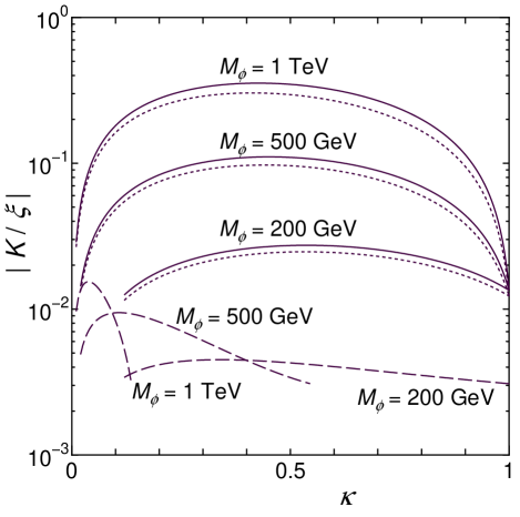
FIG. 2.: The factor $|K/\xi|$ is plotted against $\kappa$ for typical cases (A) (solid lines), (B) (dotted lines) and (C) (dashed lines).

REFERENCES

- [1] Y. Fukuda et al., Phys. Lett. B 335, 237 (1994); SuperKamiokande Collaboration, Y. Fukuda et al., Phys. Rev. Lett. 81, 1562 (1998); H. Sobel, Talk presented at Neutrino 2000, Sudbury, Canada, 2000, http://nu2000.sno.laurentian.ca/ .
- [2] Y. Suzuki, Talk presented at Neutrino 2000, Sudbury, Canada, 2000, http://nu2000.sno.laurentian.ca/ .
- [3] M. Gell-Mann, P. Ramond and R. Slansky, in : Supergravity, Proceedings of the Workshop, Stony Brook, New York,1979, eds. P. Van Nieuwenhuizen and D. Z. Freedman (North Holland, Amsterdam, 1979) p. 315; T. Yanagida, in: Proceedings of Workshop of Unified Theory and Baryon Number in The Universe, eds. O. Sawada and A. Sugamoto (KEK 1979); R. N. Mohapatra and G. Senjanovic, Phys. Rev. Lett. 44, 912 (1980); Phys. Rev. D23, 165 (1981).
- [4] C. D. Froggatt, M. Gibson and H. B. Nielsen, Phys. Lett. B 446, 256 (1999); R. Barbieri, L. J. Hall and A. Strumia, Phys. Lett. B 445, 407 (1999); R. Barbieri et al., J. High Energy Phys. 12, 017 (1998).
- [5] A. Zee, Phys. Lett. 93B, 389 (1980).
- [6] A. Yu. Smirnov and M. Tanimoto, Phys. Rev. D55, 1665 (1997).
- [7] C. Jarlskog, M. Matsuda, S. Skadhauge, M. Tanimoto, Phys. Lett. B449, 240 (1999).
- [8] P. Frampton and S. L. Glashow, hep-ph/9906375 (1999).
- [9] S. Kanemura, T. Kasai, G.-L. Lin, Y. Okada, J.-J. Tseng and C.-P. Yuan, hep-ph/0011357, (2000) .
- [10] N. Gaur, A. Ghosal, E. Ma, P. Roy, et. al, Phys. Rev. D58, 071301 (1998).
- [11] Y. Koide and A. Ghosal, Phys. Rev. D63, 037301 (2001).
- [12] Muon (g-2) Collaboration: H. N. Brown, et al., hep-ex/0102017; Phys. Rev. Lett.86, 2227 (2001).
- [13] M. Anwar Mughal, M. Sadiq and K. Ahmed, Phys. Lett. B417,87 (1998); E. J. Chun, hep-ph/0101170, J. Bordes, C. Hong-Mo, T. S. Tsun, hep-ph/0012119; E. O. Iltan, hep-ph/0101017; S. Bergmann, H. V. Klapdor-Kleingrothaus and H. Pas, hep-ph/0004048; J. I. Illana, T. Riemann, hep-ph/0010193; K. Cheung and O. C. W. Kong, hep-ph/0101347.
- [14] D. A. Dicus, H. J. He and J. N. Ng, hep-ph/0103126; E. Mituda and K. Sasaki, hep-ph/0103202.
- [15] A. Ghosal, Phys. Rev. D62, 092001 (2000).
- [16] S. T. Petcov, Phys. Lett. B115, 401 (1982).
- [17] D. E. Groom et al., (Particle Data Group), Eur. Phys. Jour. C15, 1 (2000), http://pdg.lbl.gov .
- [18] A. Czarnecki and W. J. Marciano, Nucl. Phys. (Proc. Suppl.) B76, 245 (1999); M. Davier and A. Hocker, Phys. Lett B435, 427 (1998).
- [19] F. J. Yndurain, hep-ph/0102312.