On the gravitational production of superheavy dark matter

Abstract

The dark matter in the universe can be in the form of a superheavy matter species (wimpzilla). Several mechanisms have been proposed for the production of wimpzilla particles during or immediately following the inflationary epoch. Perhaps the most attractive mechanism is through gravitational particle production, where particles are produced simply as a result of the expansion of the universe. In this paper we present a detailed numerical calculation of wimpzilla gravitational production in hybrid-inflation models and natural-inflation models. Generalizing these findings, we also explore the dependence of the gravitational production mechanism on various models of inflation. We show that superheavy dark matter production seems to be robust, with $\Omega_{X}h^{2}\sim(M_{X}/10^{11}\textrm{GeV})^{2}(T_{RH}/10^{9}\textrm{GeV})$, so long as $M_{X}<H_{I}$, where $M_{X}$ is the wimpzilla mass, $T_{RH}$ is the reheat temperature, and $H_{I}$ is the expansion rate of the universe during inflation.

I Introduction

The case for dark, nonbaryonic matter in the universe is today stronger than ever turner . The observed large-scale structure suggests that dark matter (DM) accounts for at least 30% of the critical mass density of the universe $\rho_{C}=3H_{0}^{2}M_{Pl}^{2}/8\pi=1.88\times 10^{-29}$ g cm^-3, where $H_{0}\equiv 100h$ km sec^-1 Mpc^-1 is the present Hubble constant and $M_{Pl}$ is the Planck mass.

Despite this compelling evidence, the nature of the DM is still unknown. Some fundamental physics beyond the Standard Model (SM) is certainly required to account for the cold and slowly moving particles, $X$, composing the the bulk of the nonbaryonic dark matter.

The most familiar assumption is that dark matter is a thermal relic, i.e., it was initially in chemical equilibrium in the early universe. A particle species, $X$, tracks its equilibrium abundance as long as reactions which keep the species in chemical equilibrium can proceed on a timescale more rapid than the expansion rate of the universe, $H$. When the reaction rate becomes smaller than the expansion rate, the particle species can no longer track its equilibrium value. When this occurs the particle species is said to be “frozen out.” The more strongly interacting the particle, the longer it stays in local thermal equilibrium and the smaller its eventual freeze-out abundance. Conversely, the more weakly interacting the particle, the larger its present abundance. If freeze out occurs when the particles $X$ are nonrelativistic, the freeze-out value of the particle number per comoving volume $Y$ is related to the mass of the particle and its annihilation cross section (here characterized by $\sigma_{0}$) by book $Y\propto(1/M_{X}M_{Pl}\sigma_{0})$ where $M_{X}$ is the mass of the particle $X$. Since the contribution to $\Omega_{X}=\rho_{X}/\rho_{C}$ is proportional to $M_{X}n_{X}$, which in turn is proportional to $M_{X}Y$, the present contribution to $\Omega_{X}$ from a thermal relic roughly is independent of its mass and depends only upon the annihilation cross section. The cross section that results in $\Omega_{X}h^{2}\sim 1$ is of order $10^{-37}$cm², which is of the order the weak scale. Many theories beyond the SM, e.g. supersymmetric theories, have stable particles with weak-scale annihilation cross sections, and provide candidate weakly interacting massive particles (wimps).

The simple assumption that dark matter is a thermal relic limits the maximum mass of the DM. The largest possible annihilation cross section is roughly $M_{X}^{-2}$. This implies that very massive wimps would have such a small annihilation cross section that their present abundance would be too large. Thus, one expects a maximum mass for a thermal wimp, which turns out to be a few hundred TeV griestkam .

One should note that the computation of the final abundance of the thermal relics assumes that the largest temperature of the universe was larger than the relic mass $M_{X}$. The thermal history of the universe before the epoch of nucleosynthesis is unknown, and the maximum temperature in the radiation-dominated phase, dubbed the reheating temperature ($T_{RH}$), might have been smaller than the mass of the wimp. In such a case, the dependence of the present abundance on the mass and the annihilation cross section differs from familiar results because of the new parameter $T_{RH}$ gkr . This drastically changes the cosmologically allowed parameter space of supersymmetric models and re-establishes SM neutrinos as possible dark matter candidates gkrst .

While a thermal origin for wimps is the most common assumption, it is not the simplest possibility. It has been recently pointed out that DM particles might have never experienced local chemical equilibrium during the evolution of the universe, and that their mass may be in the range $10^{12}$ to $10^{19}$ GeV, much larger than the mass of thermal wimps ckr1 ; ckr2 ; ckr3 ; ckr4 . Since these wimps would be much more massive than thermal wimps, such superheavy DM particles have been called wimpzillas ckr4 .

Since wimpzillas are extremely massive, the challenge lies in creating very few of them. Several wimpzilla scenarios have been developed involving production during different stages of the evolution of the universe.

wimpzillas may be created during bubble collisions if inflation is completed through a first-order phase transition barrow ; mr ; at the preheating stage after the end of inflation with masses easily up to the Grand Unified scale of $10^{15}$GeV Kolb:1998he or even up to the Planck scale Giudice:1999fb ; or during the reheating stage after inflation ckr3 with masses which may be as large as $2\times 10^{3}$ times the reheat temperature.

wimpzillas may also be generated in the transition between an inflationary and a matter-dominated (or radiation-dominated) universe due to the “nonadiabatic” expansion of the background spacetime acting on the vacuum quantum fluctuations. This mechanism was studied in details in Refs. ckr1 ; kuzmin in the case of chaotic inflation. The distinguishing feature of this mechanism is the capability of generating particles with mass of the order of the inflaton mass (usually much larger than the reheating temperature) even when the particles only interact extremely weakly (or not at all) with other particles, and do not couple to the inflaton.

While the results depend weakly on details such as whether the wimpzilla is a fermion or a boson, or whether it is conformally or minimally coupled to gravity, for the most part $\Omega_{X}\sim 1$ when the mass of the wimpzilla is approximately the order of the inflaton mass. Since hybrid inflation models have (at least) two mass scales and more coupling constants than chaotic inflation models, it is worthwhile to study wimpzilla production in hybrid models hybrid .

In this paper we study the gravitational production of wimpzillas after the completion of a stage of hybrid inflation. The hybrid scenario involves two scalar fields, the inflaton field $\phi$, and the symmetry-breaking field $\sigma$. Models are parameterized by different mass scales and couplings for the two fields. During inflation the inflaton field $\phi$ rolls down along a flat potential while the field $\sigma$ is stuck at the origin, providing the vacuum energy density driving inflation. However, when $\phi$ becomes smaller than a critical value, $\phi_{c}$, both fields roll down very quickly towards their present minima, completing the inflationary phase. It is exactly during this phase the gravitational generation of wimpzillas may occur.

If the wimpzillas are produced at the end of inflation, the fraction of the total energy density of the universe in wimpzillas today is given by

$$\Omega_{X}h^{2}\approx\Omega_{R}h^{2}\>\left(\frac{T_{RH}}{T_{0}}\right)\>\frac{8\pi}{3}\left(\frac{M_{X}}{M_{Pl}}\right)\>\frac{n_{X}(t_{e})}{M_{Pl}H_{I}^{2}},$$ (1)

where $H_{I}$ is the expansion rate of the universe at the end of inflation. Here, $\Omega_{R}h^{2}\approx 4.31\times 10^{-5}$ is the fraction of critical energy density in radiation today, $T_{0}$ is the present temperature of radiation, and $n_{X}(t_{e})$ is the density of $X$ particles at the time when they were produced. The present abundance of the nonthermal wimpzillas is, as expected, independent of the cross section ckr1 ; ckr2 , and one can easily verify that if there is some way to create wimpzillas in the correct abundance to give $\Omega_{X}\sim 1$, nonequilibrium during the evolution of the universe is automatic.

The paper is organized as follows. In Section II we present some details of the simplest hybrid inflation model and discuss the allowed range of the various parameters. In Section III we present our analytical results for wimpzilla production, making use of some general results presented in the appendix. Section IV contains our numerical results. Finally, in Section V we present our conclusions.

II The hybrid inflation model

For our computation of wimpzilla production, we take the simplest hybrid inflation potential as suggested by Linde hybrid

$$V(\phi,\sigma)=\frac{1}{4\lambda}\left(m_{\sigma}^{2}-\lambda\sigma^{2}\right)^{2}+\frac{1}{2}m_{\phi}^{2}\phi^{2}+\frac{1}{2}g^{2}\phi^{2}\sigma^{2}\ .$$ (2)

This potential has a valley of minima at $\sigma=0$ for $\phi>\phi_{c}\equiv m_{\sigma}/g$. Most of inflation occurs while $\phi$ is slowly rolling down from its initial value to $\phi_{c}$.

During inflation $\sigma$ has a minimum at $\sigma=0$ and its kinetic energy is quickly damped by the Hubble expansion. Hence, classically in this naive picture, $\sigma$ remains at 0 for a long time before it falls due to some infinitesimal residual displacement of $\sigma$ and/or $\dot{\sigma}$ about 0 . However, this picture is valid, strictly speaking, only when one neglects quantum fluctuations. Physically, what will occur is that the quantum fluctuations will grow and the long wavelength modes will condense such that different regions of spacetime will behave as if they had a classical scalar field value of $\sigma=\pm m_{\sigma}/\sqrt{\lambda}$ with domain walls between the plus and minus regions. (In the case that the scalar field is complex, a cosmic string will form instead of a domain wall.) This phenomenon is sometime called spinodal decomposition.

A relevant observation for gravitational particle production is that the effective stress caused by the field gradients will increase the pressure of the universe such that the Hubble expansion will slow faster. One way to see this is to note that the energy conservation equation

$$d\left(\rho a^{3}\right)=-Pd(a^{3})$$ (3)

tells us that

$$\rho=\rho_{i}\left[\frac{a_{i}}{a}\right]^{3}-\frac{1}{a^{3}}\int_{a_{i}}^{a}Pd\left[\frac{a}{a_{i}}\right]^{3},$$ (4)

which implies that a positive increase in the pressure will lead to a faster decrease in the energy density, causing a faster decrease in $H$. Of course, even if the universe contains inhomogeneities due to these field gradients, one can average over the fluctuation to account for an effective energy density and pressure.

One way of accounting for quantum fluctuations has been presented by Ref. usefulspinodal . There, the canonical formalism is used to quantize the fluctuations about a time dependent zero mode $\bar{\sigma}(t)$: $\sigma=\bar{\sigma}(t)+\delta\sigma(x,t)$. They argue that the long wavelength modes of $\delta\sigma(x,t)$ condense such as to form an effectively homogeneous scalar field $\delta\bar{\sigma}(t)$, whose energy contribution to the stress energy tensor can dominate over the stress energy of the background mode $\bar{\sigma}(t)$ such that the expansion rate $\dot{a}/a$ is damped more quickly than one would naively expect from accounting for only $\bar{\sigma}(t)$. This effectively homogeneous scalar field $\delta\bar{\sigma}(t)$ has an initial condition that is fixed by $\langle\delta\sigma^{2}(x,t)\rangle$ in the background of $\bar{\sigma}(t)$. It is

$$\langle\delta\bar{\sigma}^{2}(t_{0})\rangle^{1/2}\approx\frac{H_{I}}{2\pi},$$ (5)

where the exact numerical factor depends on the boundary condition of the quantum fluctuations (which cannot be zero due to canonical commutation relations), and $H_{I}$ is the Hubble expansion rate during inflation.

We will implement this result and simulate the condensation $\delta\bar{\sigma}$ and its fall by letting $\sigma$ have a nonzero initial condition at the end of inflation with a value of order $H_{I}/2\pi$ and letting it fall, instead of having the condensation component fall. To achieve this, we add a perturbation potential

$$V_{P}(\phi,\sigma)=BH_{I}^{3}\left(\sigma-\frac{m_{\sigma}}{\sqrt{\lambda}}\right)\,\exp\left[-C\left(\phi-\phi_{c}\right)^{2}\right].$$ (6)

Then, by adjusting $B$ and $C$ we can simulate the condensate $\delta\bar{\sigma}$ by making $\sigma(t)$ roll to the new minimum instead. We shall, however, not take into account the potential for $\delta\bar{\sigma}(t)$ as is done in Ref. usefulspinodal . In detail, if the potential for $\sigma$ is as given in Eq. (2), the potential in which $\delta\bar{\sigma}$ falls would be

$$V(\phi,\sigma)=\frac{1}{4\lambda}\left(m_{\sigma}^{2}-\lambda\bar{\sigma}^{2}\right)^{2}+\frac{1}{2}m_{\phi}^{2}\phi^{2}+\frac{1}{2}g^{2}\phi^{2}\bar{\sigma}^{2}+\frac{1}{2}\left(-m_{\sigma}^{2}+g^{2}\phi^{2}+3\lambda\bar{\sigma}^{2}\right)\delta\bar{\sigma}^{2}+\frac{3\lambda}{4}\delta\bar{\sigma}^{4},$$ (7)

where $\bar{\sigma}=0$ in our case. Comparing this expression with the tree-level effective potential, one finds that the potential for $\sigma$ with a slight displacement from $\sigma=0$ achieves the same dynamics as $\delta\bar{\sigma}(t)$ if $\lambda$ is replaced with $3\lambda$. Hence, if we only consider the case where $\sigma=0$ forever without the quantum fluctuations, our simulated treatment of spinodal decomposition will coincide with that of Ref. usefulspinodal with just the reinterpretation of $\lambda\rightarrow 3\lambda$. On the other hand, in reality, since $\sigma$ will never precisely be at zero forever even in the nonrealistic absence of quantum fluctuations, a better simulated treatment of the spinodal decomposition requires further modifications of the potential along the lines of Eq. (7) with $\bar{\sigma}\neq 0$. Since we are primarily concerned with order of magnitude accuracy, and since this approximation neglects classical wave scattering effects taken into account in Ref. lattice , we will not account for this effective change in the potential for $\sigma$.

Let us be more precise about the order of magnitude of $B$ and $C$. To displace effectively $\sigma$ by $H_{I}/2\pi$ at the end of inflation, we must have

$$B\approx\frac{10^{7}g^{2}}{\lambda}\left[\frac{m_{\sigma}}{M_{Pl}}\right]^{2}\frac{1}{\ln[1+g/\sqrt{C}m_{\sigma}]^{2}},$$ (8)

where we have used the COBE determination of curvature perturbations, giving rise to the relationship

$$m^{2}_{\phi}\approx\frac{g}{\lambda^{3/2}}\ \frac{m_{\sigma}^{5}}{3.5\times 10^{-5}M_{Pl}^{3}}.$$ (9)

Note that the precise value of $B$ and $C$ will not be important to the determination of the Bogoliubov coefficient as long as the perturbation potential causes $\sigma$ to fall. We have checked this numerically as shown below in the case where we have set $m_{\sigma}=10^{-3}M_{Pl}$.

We would like to emphasize that while our treatment of spinodal decomposition is adequate for the purposes at hand, it is far from complete. Since Ref. lattice argues that generically hybrid inflation ends after one oscillation, we cannot realistically probe the parameter space in our model where more than one oscillation of the scalar fields is important if we neglect the important pressure-related effects due to condensation and classical-wave scattering. Even for the one oscillation approximation, the effect of neglecting the pressure due to condensation and classical-wave scattering underestimates particle production due to the fact that the pressure effects increase the nonadiabticity of the expansion of spacetime. Hence, this issue certainly deserves more investigation. We note that other related references include Refs. otherspinodal1 ; otherspinodal2 ; otherspinodal3 ; otherspinodal4 and references therein.

The parameters in the potential in Eq. (2) are constrained by several considerations. Constraints on the amplitude and the tilt of the curvature perturbation spectrum generated during inflation impose the following constraints on $\lambda$ and $g$ lr :

$$\frac{g}{\lambda^{3/2}}\frac{m_{\sigma}^{5}}{m_{\phi}^{2}M_{Pl}^{3}}\approx 3.5\times 10^{-5},$$ (10)

and

$$\frac{\lambda m_{\phi}^{2}M_{Pl}^{2}}{\pi m_{\sigma}^{4}}\stackrel{{\scriptstyle<}}{{{}_{\sim}}}0.25.$$ (11)

The requirement that the cosmological constant term dominates during the inflationary regime above $\phi_{c}$ imposes a third constraint,

$$m_{\phi}^{2}\ll\frac{g^{2}m_{\sigma}^{2}}{\lambda}.$$ (12)

Note that the tilt of the curvature perturbation spectrum yields a constraint similar to the condition that the $\phi$ field evolution is slow roll; i.e.,

$$\frac{m_{\sigma}^{2}}{m_{\phi}M_{Pl}}\gg\sqrt{\frac{3\lambda}{2\pi}}.$$ (13)

Also, note that the condition that the cosmological constant term dominates during the inflationary regime with $\phi>\phi_{c}$ also implies the “waterfall” condition (the condition that the scalar fields after $\phi$ reaches $\phi_{c}$ roll to the new minima quickly compared to the expansion rate).

With $m_{\sigma}$ fixed, these constraints collectively determine a region of $(g,\lambda)$ parameter space, outside of which is forbidden by the perturbation amplitude and tilt considerations. Yet there is one other constraint that we have not discussed. As we have reviewed previously, our model does not describe the evolution of the expansion rate of the universe accurately beyond one oscillation of the scalar fields after the end of inflation. As we will see in the next section, our relic density will depend upon an accurate modeling of the background equation for at least one Hubble time at the end of inflation. Hence, our model is valid only in the regime in which no more than one oscillation takes place during one Hubble time. Let us see how this constrains our parameter space.

The time scale for the scalar field oscillation is set by the mass matrix (in the $(\sigma,\phi)$ basis)

$$m^{2}(t)=\frac{1}{2}\left(\begin{array}[]{cc}-m_{\sigma}^{2}+g^{2}\phi^{2}+3\lambda\sigma^{2}&2g^{2}\phi\sigma\\ 2g^{2}\phi\sigma&m_{\phi}^{2}+g^{2}\sigma^{2},\end{array}\right)$$ (14)

which for two extreme values of $\sigma$, $\sigma=m_{\sigma}/\sqrt{\lambda}$ and $\sigma=0$, becomes

$$m^{2}(\sigma=m_{\sigma}/\sqrt{\lambda},\phi=0)=\frac{1}{2}\left(\begin{array}[]{cc}2m_{\sigma}^{2}&0\\ 0&m_{\phi}^{2}+g^{2}m_{\sigma}^{2}/\lambda\end{array}\right)$$ (15)

and

$$m^{2}(\sigma=0,\phi)=\frac{1}{2}\left(\begin{array}[]{cc}-m_{\sigma}^{2}+g^{2}\phi^{2}&0\\ 0&m_{\phi}^{2}\end{array}\right).$$ (16)

We see that although the main oscillation frequency scale is $m_{\sigma}$, since $\phi$ can be as large as $\phi_{c}\equiv m_{\sigma}/g$ and since typically $m_{\phi}\ll m_{\sigma}$, the actual frequency scale for the oscillation will be a weighted time average,whose value can be significantly lower than $m_{\sigma}$. Let us call this weighted average frequency scale $m_{\sigma}f$, where $f<1$ is some constant (typically $f$ is of order $10^{-3})$. As far as the Hubble expansion rate at the end of inflation is concerned, in the model we study it is given by

$$H_{I}\equiv\sqrt{\frac{2\pi}{3\lambda}\frac{m_{\sigma}^{4}}{M_{Pl}^{2}}}=1.8\times 10^{14}\left(\frac{m_{\sigma}}{10^{-3}M_{Pl}}\right)^{2}\left(\frac{10^{-2}}{\lambda}\right)^{1/2}\textrm{GeV}.$$ (17)

Then, the ratio

$$\frac{H_{I}}{fm_{\sigma}}=\sqrt{\frac{2\pi}{3\lambda}}\ \frac{m_{\sigma}}{fM_{Pl}}$$ (18)

implies that unless $m_{\sigma}$ is within a factor of $f\sqrt{\lambda}$ of $M_{Pl}$, many oscillations will occur during the one Hubble time when particle production occurs. Hence, the constraint on our parameter space due to limitations of our background field model is that $m_{\sigma}$ be as close to as $M_{Pl}$ as possible. Since Planckian energy densities invalidate semi-classical gravitational physics, we will set $m_{\sigma}$ at the GUT scale,

$$m_{\sigma}=10^{-3}M_{Pl},$$ (19)

assuming that there is some physics separating the GUT scale and the quantum gravity scale. Hence, the following interesting set of parameters ($g=0.01$, $\lambda=1$, $m_{\sigma}=10^{-7}M_{Pl}$, $m_{\phi}\approx 652$ GeV) which satisfy all the constraints and give a mass scales in the intermediate scale $(10^{12}$ GeV) and the electroweak scale, cannot be analyzed in our model because in this case, $H_{I}/(fm_{\sigma})$ is too small. In fact, even for the single oscillation case, there may be some other damping factor for $\dot{\phi}$ and $\dot{\sigma}$ which affects the magnitude of $\dot{H}$, which of course is crucial for the particle production calculation (as we will explain further in the next section). Hence, we consider even the numerical calculation results in this article to be only order of magnitude accurate.

Before we map out the parameter space for which our calculation explicitly is valid, we would like to show that having $m_{\sigma}$ close to $M_{Pl}$ forces the scalar fields to have Planck scale vevs. This is noteworthy. Because of the possible sensitivity to unknown Planck-suppressed operators, scenarios in which the inflaton attains a Planck scale vev may be unattractive lyth .

We can model the dynamics of $\phi$ before reaching $\phi_{c}$ as the evolution of a non-interacting inflaton in a de Sitter background:

$$\ddot{\phi}+3H\dot{\phi}+m_{\phi}^{2}\phi=0.$$ (20)

For the inflaton field to be slow rolling (overdamped) to the critical value $\phi_{c}$ from some initial value of $\phi(t=0)>\phi_{c}$, we must have $m_{\phi}/H\ll 1$. In that case, taking the least damped solution, we have

$$\phi=\phi_{c}\exp\left[\frac{1}{3}\left(\frac{m_{\phi}}{H_{I}}\right)^{2}H_{I}\left(t_{c}-t\right)\right].$$ (21)

Note that since $\phi_{c}=m_{\sigma}/g$, having $m_{\sigma}$ close to the Planck scale means that $\phi_{c}$ will be close to the Planck scale. We can be more quantitative by seeing what the constraint $\phi(t=0)<cM_{Pl}$ with $c$ of order unity implies. Since $a(t)/a(t=0)=\exp(H_{I}t)$, to have $60$ e-folds, we must have $\phi(t=0)>\phi_{c}\exp\left[60\left(m_{\phi}/H_{I})^{2}/3\right)\right]$. This implies

$$\frac{m_{\phi}M_{Pl}}{m_{\sigma}^{2}}\sqrt{\frac{30\lambda}{\pi}}<\sqrt{\ln\left(\frac{cgM_{Pl}}{m_{\sigma}}\right)},$$ (22)

where we have taken $\phi_{c}=m_{\sigma}/g$. There are instances when this constraint becomes independent of other constraints. For example, $g=10^{-4},\,\lambda=1,\,m_{\sigma}=10^{-4}M_{Pl},\,m_{\phi}=1.7\times 10^{9}$ GeV satisfies all other conditions but this one with $c=1$. We will neglect this “small field” constraint since this is not as fundamental as other constraints.

In summary, the parameter space that we will explore will be

$$\frac{3\times 10^{-5}}{\sqrt{\lambda}}\ll g\stackrel{{\scriptstyle<}}{{{}_{\sim}}}3\times 10^{-2}\sqrt{\lambda}$$ (23)

The parameter space is shown explicitly in Fig. 1.

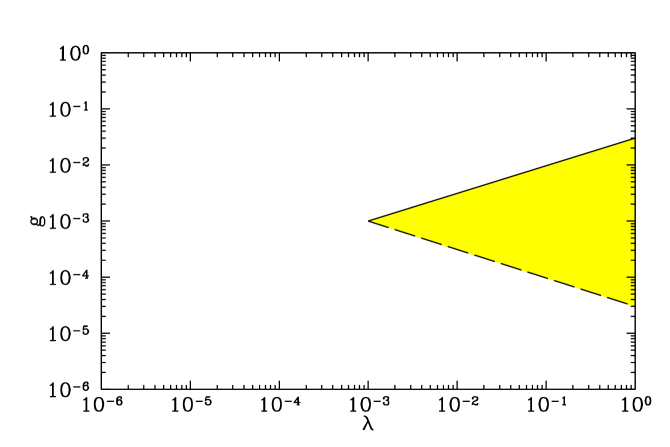
Figure 1: The $\lambda$-$g$ parameter space in hybrid inflation. The shaded region corresponds to values of the parameters allowed by Eqs. (10 - 12). The lower limit on this region is dashed because it represents the ”$\gg$” limit in Eq. (23).

III analytic estimate of particle production

In the appendix we present a general method of estimating particle production from strong gravitational fields. In this section we apply the results from the appendix to the hybrid inflationary scenario.

We show in the appendix that an estimate of particle production requires an estimate of the background equation solutions. To start off, let us examine the time variation of $\dot{H}/H$. After inflation as the scalar fields oscillate about their minima, $\dot{H}/H$ oscillates. For the envelope of the function describing the oscillations we have

$$\dot{H}=-\frac{4\pi}{M_{Pl}^{2}}(\dot{\phi}^{2}+\dot{\sigma}^{2})\approx-\frac{4\pi}{M_{Pl}^{2}}\rho$$ (24)

and the Friedmann equation,

$$H^{2}=\frac{8\pi}{3M_{Pl}^{2}}\rho.$$ (25)

From these, we find a following general relationship after the end of inflation

$$\left.\dot{H}\right|_{\textrm{envelope}}\sim H^{2}.$$ (26)

In fact, after the first oscillation the scalar fields will undergo damped oscillation about their new minimum, and the scale factor during that time varies in general as

$$a(t)=a_{e}\left(\frac{t}{t_{e}}\right)^{\alpha}$$ (27)

where in the hybrid inflationary case, $\alpha\approx 2/3$ (which is a typical result of massive scalar field oscillation). In reality, this $\alpha$ will have corrections coming from the phase transition physics.

Before inflation ends, the scale factor will be taken to evolve as

$$a(t)=a_{e}\exp\left[H_{I}\left(t-t_{e}\right)\right]$$ (28)

with $H_{I}$ given by Eq. (17).

Let us now follow the procedure outlined in the appendix to calculate $n_{X}(t_{e})$. First, consider the contribution to modes that are nonrelativistic at the end of inflation, $I_{a}(k)+I_{b}(k)$, given in Eq. (53). Assuming $H_{I}$ is a constant and $a(t)$ evolves as Eq. (28),we find

$$I_{a}(k)=\frac{1}{4}\ \frac{M_{X}^{2}}{k^{2}}\ a_{e}^{2}\left[e^{2H_{I}\left(t_{2}-t_{e}\right)}-e^{2H_{I}\left(t_{1}-t_{e})\right)}\right],$$ (29)

where, from the Appendix $t_{1}$ and $t_{2}$, are defined by

$$k_{\textrm{physical}}(t_{1})=\frac{k}{a_{e}}\ \frac{a_{e}}{a(t_{1})}=2H_{I}$$

$$k_{\textrm{physical}}(t_{2})=\frac{k}{a_{e}}\ \frac{a_{e}}{a(t_{2})}=M_{X}.$$ (30)

Hence, we obtain for $I_{a}(k)$ the result

$$I_{a}(k)=\frac{1}{4}\left[1-\left(\frac{M_{X}}{2H}\right)^{2}\right].$$ (31)

Next, we calculate the nonrelativistic contribution in the period after inflation, $I_{b}(k)$, also defined in Eq. (53). Since $t_{4_{i}}$ and $t_{3_{i+1}}$ are close together, ($t_{3_{i+1}}-t_{4_{i}}\ll 1/H$) for $M_{X}/H\ll 1$, and since we are concerned with order of magnitudes, we can just integrate from $t_{3_{1}}$ to $t_{4_{N}}$ instead of summing over each $i$. Since the nonadiabatic region begins at around $t_{e}$, we take $t_{3_{1}}\approx t_{e}$. The final integration time, $t_{4_{N}}$, is defined by the condition $|\dot{H}/H|>M_{X}$. In the period after inflation we will take $a(t)\propto t^{\alpha}$ as in Eq. (27), so $H=\alpha/t$ and $\dot{H}/H=1/t$. Hence, we have

$$I_{b}(k)=\frac{1}{2}\int_{t_{e}}^{t_{4_{N}}}\ H(t)\ dt=\frac{\alpha}{2}\ln\left(\frac{t_{4_{N}}}{t_{e}}\right)=\frac{\alpha}{2}\ln\left(\frac{H_{I}}{M_{X}\alpha}\right).$$ (32)

The calculation of the production of modes relativistic at the end of inflation, $J_{a}(k)+J_{b}(k)$ given in Eq. (54), is a bit trickier. First of all, consider the contribution $J_{a}(k)$:

$$J_{a}(k)=\frac{1}{2}\int_{t_{5}}^{t_{6}}dt\ \frac{a^{2}(t)}{q^{2}}H(t),$$ (33)

where $t_{5}$ is the time during inflation when $k_{\textrm{physical}}(t_{5})=2H_{I}$. During inflation $a(t)=a_{e}\exp\left[H_{I}(t-t_{e})\right]$, and $k_{\textrm{physical}}(t_{5})=2H_{I}$ gives

$$\frac{k}{a(t_{5})}=ka_{e}\exp\left[-H_{I}(t_{5}-t_{e})\right]=2H_{I}.$$ (34)

The time $t_{6}$ is the smallest of the times after inflation when $k_{\textrm{physical}}(t_{6})=2H$ or $k_{\textrm{physical}}(t_{6})=M_{X}$. In the period after inflation, $a(t)=(t/t_{e})^{\alpha}$ and $H=\alpha/t$, so

$$\frac{t_{6}}{t_{e}}=\textrm{MIN}\left[\left(\frac{q/a_{e}}{2H_{I}/M_{X}}\right)^{1/(\alpha-1)},\left(\frac{q}{a_{e}}\right)^{1/\alpha}\right],$$ (35)

where the first term is $k_{\textrm{physical}}(t_{6})=2H$ and the second term is $k_{\textrm{physical}}(t_{6})=M_{X}$.

Since $t_{6}$ will occur after inflation, $J_{a}(k)$ divides into the parts before and after inflation:

$$J_{a}(k) = \frac{1}{2}\frac{H_{I}}{q^{2}}\int_{t_{5}}^{t_{e}}dt\ a^{2}(t)+\frac{1}{2}\frac{1}{q^{2}}\int_{t_{e}}^{t_{6}}dt\ a^{2}(t)H(t)$$ (36)

$$= \frac{1}{4}\left[1-\left(\frac{M_{X}}{2H_{I}}\right)^{2}\right]\theta\left[\left(\frac{2H_{I}}{M_{X}}\right)^{\alpha}-\frac{q}{a_{e}}\right]$$

$$+\frac{1}{4}\left[\frac{\left(2H_{I}/M_{X}\right)^{2\alpha/(1-\alpha)}}{(q/a_{e})^{2/(1-\alpha)}}-\left(\frac{M_{X}}{2H_{I}}\right)^{2}\right]\theta\left[\frac{q}{a_{e}}-\left(\frac{2H_{I}}{M_{X}}\right)^{\alpha}\right]\theta\left(\frac{2H_{I}}{M_{X}}-\frac{q}{a_{e}}\right).$$

where $\theta$ is a step function. The second theta function in the second term ensures that $t_{6}/t_{e}>1$. Note that $J_{a}$ matches $I_{a}$ in the limit $q/a_{e}\rightarrow 1$.

To calculate $J_{b}$, we follow the similar procedure as we did for $I_{b}$, and integrate from $t_{7_{1}}=t_{6}$ to $t_{8_{N}}=t_{4_{N}}$. Note that this is nonzero only when $t_{7_{1}}\leq t_{8_{N}}$. Hence, we have

$$J_{b}=\left[\frac{\alpha}{2}\ln\left(\frac{H_{I}}{M_{X}\alpha}\right)-\frac{1}{2}\ln\left(\frac{q}{a_{e}}\right)\right]\theta\left[\left(\frac{H_{I}}{\alpha M_{X}}\right)^{\alpha}-\frac{q}{a_{e}}\right]\theta\left[\left(\frac{2H_{I}}{M_{X}}\right)^{\alpha}-\frac{q}{a_{e}}\right].$$ (37)

The first $\theta$ comes from $t_{7_{1}}<t_{8_{N}}$ and the second $\theta$ comes from using $t_{7_{1}}=t_{6}=t_{e}\left(q/a_{e}\right)^{1/\alpha}$ (see Eq. 35). Note that $t=t_{e}\left(q/a_{e}\right)^{1/\alpha}$ is the time at which the momentum becomes nonrelativistic, and it is precisely this regime during which $J_{b}$ is calculated. If $q/a_{e}>\left(2H_{I}/M_{X}\right)^{\alpha}$, then the momentum becomes relativistic and there is no extra contribution to $J_{b}$. From now on we will assume that $\alpha\geq 1/2$, in which case the second $\theta$ function is irrelevant.

Writing

$$\beta_{q}=(I_{a}+I_{b})\,\theta(1-q/a_{e}+\epsilon)+(J_{a}+J_{b})\,\theta(q/a_{e}-1)$$ (38)

where the $\epsilon$ indicates that we take the first term when $q/a_{e}=1$, we can finally obtain the number density $n_{X}(t_{e})$ through

$$n_{X}(t_{e}) = \frac{M_{X}^{3}}{2\pi^{2}}\int d\left(\frac{q}{a_{e}}\right)\left(\frac{q}{a_{e}}\right)^{2}\left|\beta_{q}\right|^{2}$$ (39)

$$= \frac{H_{I}^{3}z^{3}}{2\pi^{2}}\left[\frac{1}{48}\left(1-\frac{z^{2}}{4}\right)^{2}+\frac{\alpha^{2}}{12}\ln^{2}(\alpha z)+A_{1}+A_{2}+B_{1}\right],$$

where $z\equiv M_{X}/H_{I}$ and $\alpha=2/3$ in our case. The first two terms are the nonrelativistic contribution, and the relativistic contributions $A_{i}$ and $B_{1}$ are

$$A_{1} = \frac{(z^{2}-4)^{2}}{768}\left[\left(\frac{2}{z}\right)^{3\alpha}-1\right]$$ (40)

$$= \frac{0.08}{z^{2}}-0.06-0.02z^{2}+0.001z^{4}\qquad(\textrm{for }\alpha=2/3),$$

$$A_{2} = \frac{1}{768(9\alpha^{2}-1)}\left\{64z+\left[-24(1+3\alpha)(1-\alpha)z^{2}+(1+3\alpha)(1-3\alpha)z^{4}\right.\right.$$ (41)

$$\left.\left.-48(1-3\alpha)(1-\alpha)\right]\left(\frac{2}{z}\right)^{3\alpha}\right\}$$

$$= \frac{0.03}{z^{2}}-0.04+0.03z-0.005z^{2}\qquad(\textrm{for }\alpha=2/3),$$

and

$$B_{1} = \frac{1}{54}\left[\left(\frac{1}{\alpha z}\right)^{3\alpha}-1\right]+\frac{\alpha\ln(z)}{18}-\frac{\alpha^{2}\ln(\alpha)\ln(z)}{6}-\frac{\alpha^{2}\ln^{2}(z)}{12}+\frac{\alpha\ln(\alpha)}{18}-\frac{\alpha^{2}\ln^{2}(\alpha)}{12}$$ (42)

$$= \frac{0.04}{z^{2}}-0.04+0.07\ln(z)-0.04\ln^{2}(z)\qquad(\textrm{for }\alpha=2/3).$$

We have neglected cross terms as well since we have neglected any phase information (i.e., if $\beta_{q}=J_{a}+J_{b}$, then $|\beta_{q}|^{2}$ was taken to be $J_{a}^{2}+J_{b}^{2}$, which should give a lower bound and the correct order of magnitude since both $J_{a}$ and $J_{b}$ are positive). The important result is that for small $z$, one can approximate

$$\frac{1}{48}\left(1-\frac{z^{2}}{4}\right)^{2}+\frac{\alpha^{2}}{12}\ln^{2}(\alpha z)+A_{1}+A_{2}+B_{1}\approx\frac{0.15}{z^{2}}.$$ (43)

In the $z<1$ limit, the largest contribution comes from the $J_{a}(k)$ and $J_{b}(k)$ terms. This corresponds to production of modes that are relativistic at the end of inflation, with approximately equal contributions to the final value of $|\beta|^{2}$ coming just before and just after the end of inflation. We see how the exact behavior of $\dot{H}/H$ after inflation is important.

Finally, putting everything together, in the limit $z=M_{X}/H_{I}\ll 1$:

$$\Omega_{X}h^{2} \approx \Omega_{R}h^{2}\left(\frac{T_{RH}}{T_{0}}\right)\frac{8\pi}{3}\frac{zn_{X}(t_{e})}{M_{Pl}^{2}H_{I}}$$ (44)

$$\approx \left(\frac{M_{X}}{10^{11}\textrm{GeV}}\right)^{2}\left(\frac{T_{RH}}{10^{9}\textrm{GeV}}\right)\qquad(\textrm{general result})$$

$$\approx 2\times 10^{4}\left(\frac{T_{RH}}{10^{9}\textrm{GeV}}\right)\left(\frac{m_{\sigma}}{10^{-3}M_{Pl}}\right)^{4}\frac{z^{2}}{\lambda}\qquad(\textrm{hybrid inflation}),$$

where the expression is valid only if $M_{X}<H_{I}=1.8\times 10^{14}(m_{\sigma}/10^{-3}M_{Pl})^{2}(10^{-2}/\lambda)^{1/2}\textrm{GeV}$. As shown in the next section, the numerical results corroborate this analytic estimate.

Note that with $M_{X}\sim 10^{13}\textrm{GeV}$ and $T_{RH}\sim 10^{4}\textrm{GeV}$, we have $\Omega_{X}h^{2}$ of order $10^{-1}$. Characteristic of gravitational production, it is possible to produce dark matter many orders of magnitude in excess of $T_{RH}$.

We have left the $\alpha$ dependence in most of the expressions to indicate that the mass scaling is sensitive to the fact that the scalar fields enter a regime just after inflation in which the scale factor evolves as a matter-dominated universe. The physics of the spinodal decomposition is expected to change this effective $\alpha$, but one would generically expect $\alpha$ somewhere between $1/2$ and $2/3$, which means that the number density of particles produced will roughly remain the same. Hence, even though all of our calculations have some sensitivity to more than one oscillations (as can be seen in our estimation procedure), as long as the scale factor enters a scaling regime at the end of inflation, our results will give the correct order of magnitude.

IV numerical calculation of particle production

In this section we describe the results of our numerical analysis of gravitational particle production in the hybrid inflation model. The basic hybrid potential was given in Eq. (2). As discussed above, the end of inflation is triggered by some perturbation, which we model by adding to the basic potential a “perturbed” potential given in Eq. (6). The first issue is whether our results are sensitive either to the nature of the end of inflation or the way we model it.

A straightforward exercise is to investigate the sensitivity of particle production to the parameters $B$ and $C$ in the perturbed potential we use to trigger the end of inflation. In Fig. 2 we show the time evolution of the Bogoliubov coefficient for different choices of $B$ and $C$. As shown in the figure, our results are insensitive to $B$ and $C$ as long as they are chosen so as to make $V_{P}$ negligible outside a very small region around $\phi=\phi_{c}$. Note that we also set $m_{\sigma}=10^{-3}M_{Pl}$ for all the numerical work.

Figure 2: The absolute square of the Bogoliubov coefficient as a function of time for several different values of $B$ and $C$ ($B$ is dimensionless and $C$ is in units of $M_{Pl}^{2}$.) We have $g=0.01$, $\lambda=1$, $M_{X}=0.1H_{0}$, and $k=0.1a_{i}H_{0}$. The lines correspond to the deformation parameters $(B,C)$ given by $(1,10^{9})$; $(10^{3},10^{7})$; $(10^{5},10^{3})$; $(10^{5},10^{5})$; $(10^{5},10^{7})$; $(10^{5},10^{9})$. The lines are hard to distinguish on this scale and asymptotically approach within 10% of each other.

The fact that the final results are insensitive to the exact values of $B$ and $C$ suggests (but of course does not guarantee) that gravitational particle production in hybrid inflation will be independent of the mechanism that triggers the end of inflation.

The evolution of the background fields $\sigma$ and $\phi$ determine the expansion rate and the change in the expansion rate. Figure 3 is an example of the evolution of the two fields in hybrid inflation. For the parameters of this model ($g=0.01$, $\lambda=1$), the critical value of $\phi$ is $\phi_{c}=0.1M_{Pl}$. An instability in the trigger field $\sigma$ (driven by the “perturbed” potential) causes $\sigma$ and $\phi$ to evolve rapidly to their minima ($\phi=0$, $|\sigma|=m_{\sigma}/\sqrt{\lambda}=1$) once $\phi<\phi_{c}$.

Figure 3: An example of the evolution of the inflaton field $\phi$ (solid) and $\sigma$ (dashed) as a function of time at the end of hybrid inflation. The parameters chosen were $g=0.01$ and $\lambda=1$.

Figure 4: The gravitational production of particles during hybrid inflation as a function of $\lambda$, with $g$ set to $0.001$. The curves correspond to $\lambda$ as follows: solid, $\lambda=0.001$; dots, $\lambda=0.01$; dashes, $\lambda=0.1$; dash-dot, $\lambda=1$. The magnitude of $\Omega_{X}h^{2}(T_{RH}/10^{9}\textrm{GeV})^{-1}$ scales roughly as $\lambda^{-1}$.

Figure 5: The gravitational production of particles during hybrid inflation as a function of $g$, with $\lambda$ set to $1$. The curves correspond to $g$ as follows: solid, $g=1$ (note that this is outside the allowed region of $g,\lambda$ parameter space); dots, $g=0.01$; and dashes, $g=0.001$.

Figure 6: gravitational production of particles during natural inflation, with $\Lambda=10^{-3}M_{Pl}$ and $f_{\phi}=0.6M_{Pl}$.

To calculate the relic density of stable particles produced gravitationally, we integrated the background and X-particle mode equations for several different points within the allowed regions of parameters shown in Fig. 1, as well as for $\lambda=g=1$, which is well outside it. Our results are summarized in Figs. 5 and 5.

All the curves look similar in form to the mass spectrum for chaotic inflation with a potential $V(\phi)\sim m_{\phi}^{2}\phi^{2}$. The value of $\Omega_{X}h^{2}$ increases with $z=M_{X}/H_{I}$ for $z<1$, then decreases exponentially for $z>1$. The reason for this behavior is discussed in this paper for the small-$z$ region, and in dcthesis in the large-$z$ limit.

The numerical results are in qualitative agreement with the result of Eq. (44).

As another example of a single-field model, in Fig. 6, we show the mass spectrum for natural inflation natural . In natural inflation the potential is usually chosen to be

$$V(\phi)=\Lambda^{4}\left[1-\cos\left(\phi/\sqrt{2}f_{\phi}\right)\right].$$ (45)

Normalizing the parameters to produce the observed temperature fluctuations, a reasonable choice of parameters is $\Lambda=10^{-3}M_{Pl}$ and $f_{\phi}=0.6M_{Pl}$. With these choices, $H_{I}=5.1\times 10^{-7}M_{Pl}$.

As in the hybrid inflation case, in the low-$z$ limit $\Omega_{X}h^{2}\propto M_{X}^{2}$. Again, the numerical results are reasonably represented by $\Omega_{X}h^{2}\sim(M_{X}/10^{11}\textrm{GeV})^{2}(T_{RH}/10^{9}\textrm{GeV})$.

V Conclusions

The expansion rate of the universe during inflation, $H_{I}$, may signal a new mass scale in physics. The particle spectrum of this new mass scale is completely unknown. There may be no particles with this new mass scale; an example of such a model is $\phi^{4}$ chaotic inflation. There may be only one particle with this mass scale; for example, the inflaton mass in $\phi^{2}$ chaotic inflation. Nevertheless, it is very reasonable that one might expect a rich spectrum of particles of this mass scale. If this is the case, there may be nearly stable particles of this mass scale models . Independently of the coupling of the stable particle, they will be produced as a result of the expansion of the universe acting on vacuum quantum fluctuations. It was shown in Refs. ckr1 ; ckr2 ; kuzmin that such particles would be excellent candidates for dark matter. Since the dark-matter particle would have a much larger mass than usual thermal wimps, they have been named wimpzillas.

The wimpzilla scenario for dark matter seems to be quite robust. The wimpzilla may be minimally coupled or conformally coupled, it may be a boson or a fermion, it may couple to the inflaton or may be uncoupled.

The sensitivity of wimpzilla production to the inflation model is one of the subjects of this paper. Previous calculations have employed a chaotic inflation model. Here, we extend our studies on wimpzilla production to hybrid models and natural-inflation models. We have also developed analytic techniques that should provide reasonable estimates for wimpzilla production in the limit that $M_{X}<H_{I}$.

The general picture for wimpzilla production now emerges, and it seems to be relatively insensitive to the inflation model. The characteristic expansion rate during inflation, $H_{I}$, controls the maximum mass that efficiently can be produced. In all inflation models with continuous $\dot{H}$, the production of particles with mass larger than $H_{I}$ is exponentially suppressed. For particles of mass smaller than $H_{I}$, the contribution to $\Omega_{X}h^{2}$ is $(M_{X}/10^{11}\textrm{GeV})^{2}(T_{RH}/10^{9}\textrm{GeV})$.

This last expression for $\Omega_{X}h^{2}$ well illustrates that wimpzilla masses much in excess of the reheat temperature may be dark matter. For instance, if $T_{RH}=10^{4}$GeV, then $M_{X}=10^{13}$GeV would give $\Omega_{X}h^{2}$ in the desirable range.

While interesting behavior after inflation like preheating or spinodal decomposition in the case of hybrid inflation might change the results, we expect the order of magnitude estimate to be correct, and for it to be an underestimate of wimpzilla production.

Appendix A analytic determination of particle production

Consider a minimally coupled scalar field with mass $M_{X}$. The equation of motion for the field is

$$\ddot{X}+3H\dot{X}-\frac{1}{a^{2}}\nabla^{2}X+M_{X}^{2}X=0,$$ (46)

where $H$ is the expansion rate. The scalar field may be expressed in terms of Fourier modes $X_{k}=h_{k}/a$ ($a$ is the scale factor) as

$$X=\int\frac{d^{3}\!k}{(2\pi)^{3/2}a}\left[a_{k}e^{i\vec{k}\cdot\vec{x}}h_{k}(t)+a_{k}^{\dagger}e^{-i\vec{k}\cdot\vec{x}}h_{k}^{*}(t)\right],$$ (47)

with the usual normalization condition of the creation and annihilation operators, $\left[a_{\vec{k}},a^{\dagger}_{\vec{l}}\right]=\delta^{3}(\vec{k}-\vec{l})$, the mode functions $h_{k}$ satisfies the equation

$$\ddot{h}_{k}+H\dot{h}_{k}+\left[-H^{2}-\frac{\ddot{a}}{a}+\left(\frac{k}{a}\right)^{2}+M_{X}^{2}\right]h_{k}=0.$$ (48)

In terms of Bogoliubov coefficients $\alpha_{k}$ and $\beta_{k}$, the mode functions can be written as

$$h_{k}=\frac{\alpha_{k}}{\sqrt{2\omega_{k}}}\exp\left(-i\int\omega_{k}\ a^{-1}(t)\ dt\right)+\frac{\beta_{k}}{\sqrt{2\omega_{k}}}\exp\left(-i\int\omega_{k}\ a^{-1}(t)\ dt\right),$$ (49)

where $\omega_{k}^{2}=k^{2}+M_{X}^{2}a^{2}$. Solving for the mode functions is equivalent to solving the system

$$\dot{\alpha}_{k} = \frac{\dot{\omega_{k}}}{2\omega_{k}}\exp\left(2i\int\omega_{k}\ a^{-1}(t)\ dt\right)\beta_{k}$$

$$\dot{\beta}_{k} = \frac{\dot{\omega_{k}}}{2\omega_{k}}\exp\left(2i\int\omega_{k}\ a^{-1}(t)\ dt\right)\alpha_{k}.$$ (50)

The gravitational production of particles can be expressed in terms of the Bogoliubov coefficient $\beta_{k}$ as

$$n_{X}=\frac{1}{2\pi^{2}a^{3}}\int_{0}^{\infty}dk\ k^{2}\left|\beta_{k}\right|^{2}=\frac{M_{X}^{3}}{2\pi^{2}a^{3}}\int_{0}^{\infty}dq\ q^{2}\left|\beta_{q}\right|^{2},$$ (51)

where $q\equiv k/M_{X}=k_{\textrm{physical}}a/M_{X}$ with $k$ the comoving momentum and $k_{\textrm{physical}}=k/a$ the physical momentum.

The Bogoliubov coefficient to leading adiabatic order can be expressed as (see Ref. dcthesis and references therein)

$$\beta_{q}(t)\approx\int_{-\infty}^{t}dt^{\prime}\ \frac{1}{2}\left[\frac{H(t^{\prime})}{1+q^{2}/a^{2}(t^{\prime})}\right]\exp\left(-2iM_{X}\int^{t^{\prime}}_{-\infty}dt^{\prime\prime}\sqrt{1+q^{2}/a^{2}(t^{\prime\prime})}\right).$$ (52)

This formula breaks down when $|\beta|$ is of order unity (which may occur in our scenario), but let us use it to estimate the order of magnitude scales.

The magnitude of $\beta_{q}$ depends on the magnitude of the argument of the exponential in Eq. (52). If the argument is of order unity or greater, then the oscillatory behavior will damp $\left|\beta_{q}\right|$. Thus, the final magnitude of $\beta_{q}$ depends on the size of $q/a(t)$. This leads to a natural division of particle production into the cases where $q/a(t)=k_{\textrm{physical}}/M_{X}$ is larger or smaller than unity. We will consider the two cases in turn.

First consider production of nonrelativistic particles: $q/a(t)=k_{\textrm{physical}}/M_{X}<1$. This case further splits into two subclasses.

$M_{X}<|\dot{H}/H|$: In this case, the oscillations are not important, and one simply integrates $H(t)$ to the point that it becomes negligible.

$M_{X}>|\dot{H}/H|$: In this case, the oscillations cancel most of the contribution to the integrand.

Now consider production of relativistic particles: $q/a(t)=k_{\textrm{physical}}/M_{X}>1$. In this case, the frequency of the oscillations just becomes the physical momentum. Again, this case divides into two subclasses.

$k_{\textrm{physical}}<|\dot{A}/A|$, where $A(t)\equiv H(t)/\left[1+q^{2}/a^{2}(t)\right]$: Since $q/a(t)>1$, this is equivalent to $k_{\textrm{physical}}<\left|2H+\dot{H}/H\right|$. In this case the oscillations are not important, and one simply integrates $H(t)/[q^{2}/a^{2}(t)]$ to the point that it becomes negligible.

$k_{\textrm{physical}}>\left|2H+\dot{H}/H\right|$: In this case the oscillations cancel most of the contribution to the integral.

We will neglect the marginal case of $q/a=1$, since this will be roughly accounted for in the estimates of the above cases. The different cases and subcases are given in Table 1.

Table 1: This table summarizes the different cases in the analytic calculation of gravitational production of particles.

relativistic/nonrelativistic	subcase	oscillations	$\beta$
nonrelativistic	$M_{X}<|\dot{H}/H|$	none	$\int dtH(t)$
nonrelativistic	$M_{X}>|\dot{H}/H|$	many	damped
relativistic	$k_{\textrm{physical}}<\left|2H+\dot{H}/H\right|$	none	$\int dtH(t)\left[q/a(t)\right]^{-2}$
relativistic	$k_{\textrm{physical}}>\left|2H+\dot{H}/H\right|$	many	damped

A key to developing analytic approximations is the behavior of $H$ and $|\dot{H}/H|$. During inflation, $H$ is roughly constant (denoted as $H_{I}$) and $\dot{H}/H\ll H_{I}$. After inflation, $\dot{H}/H$ is negative, and oscillates (with decreasing amplitude) between zero and approximately $-H$. This behavior is illustrated in Fig. 7 in the simple chaotic inflation scenario. During the matter-dominated (MD) phase and the radiation-dominated (RD) phase, $\dot{H}/H=-3H$ and $\dot{H}/{H}=-4H$, respectively, so $\left|2H+\dot{H}/H\right|=$[1 (MD) or 2 (RD)]$\times H$

Figure 7: The behavior of $\dot{H}/{H}$ and the inflaton field at the end of inflation in a simple chaotic inflation model ($V\sim M_{\phi}^{2}\phi^{2}$). Notice the oscillatory behavior of $\dot{H}/{H}$ after inflation.

Since $\dot{H}/{H}\simeq 0$ during inflation, from Table 1 we see that production of nonrelativistic particles is suppressed during inflation and production of relativistic particles during inflation is suppressed if $k_{\textrm{physical}}\gg H$.

Let us now turn to the estimate of the number density. The particular inflation model, together with the behavior of the expansion rate immediately after inflation, will determine the efficiency of gravitational particle production. Here we will give a recipe that can be adapted for several models.

We are mainly concerned with the case when $M_{X}/H_{I}<1$. (Particle production is exponentially suppressed for $M_{X}/H_{I}>1$: this case was addressed in detail in Ref. dcthesis .) The result will depend on whether the particle was relativistic or nonrelativistic at the end of inflation.

First, consider momentum modes where the particle was nonrelativistic at the end of inflation, $k_{\textrm{physical}}(t_{e})\leq M_{X}$. The calculation divides into production during inflation and post-inflation production. During inflation, the growth in $|\beta_{k}|$ is only when $M_{X}<k_{\textrm{physical}}<2H_{I}$. After inflation, the particle is nonrelativistic, and growth occurs during periods when $M_{X}<\dot{H}/H$. Using the results summarized in Table 1 (recall that $k_{\textrm{physical}}=k/a=M_{X}q/a$),

$$\beta_{k}(k_{\textrm{physical}}(t_{e})<M_{X}) \simeq \frac{1}{2}\int_{t_{1}}^{t_{1}<t_{2}\leq t_{e}}dt\ \frac{H(t)}{q^{2}/a^{2}(t)}+\sum_{i}\frac{1}{2}\int_{t_{3_{i}}}^{t_{4_{i}}}dt\ H(t)$$ (53)

$$\equiv I_{a}+I_{b}.$$

Here, $I_{a}$ is the growth during inflation in the interval $\{t_{1},t_{2}\}$ where the times are defined such that $k_{\textrm{physical}}(t_{1})=2H_{I}$ and $k_{\textrm{physical}}(t_{2})=M_{X}$. $I_{b}$ is the growth after inflation in the intervals $\{t_{3_{i}},t_{4_{i}}\}$ when $M_{X}\leq\dot{H}/H$.

Note that we have neglected any phase information between various contributions. These interfererence terms should be important in only some special cases and not generically because in most cases only one term will dominate.

Now, consider momentum modes where the particle was relativistic at the end of inflation, $k_{\textrm{physical}}(t_{e})\geq M_{X}$. Since the mode was relativistic at the end of inflation, it must have been relativistic throughout inflation. From Table 1 we see that during inflation, the growth in the amplitude of $\beta_{k}$ only occur when $2H_{I}>k_{\textrm{physical}}$. After inflation, the mode will remain relativistic so long as $k_{\textrm{physical}}>M_{X}$ and it will continue to grow so long as $2H>k_{\textrm{physical}}$. After the mode becomes nonrelativistic ($k_{\textrm{physical}}<M_{X}$) it will grow only during periods when $M_{X}<\dot{H}/H$. Using the results summarized in Table 1 (recall that $k_{\textrm{physical}}=k/a=M_{X}q/a$),

$$\beta_{k}(k_{\textrm{physical}}(t_{e})>M_{X}) \simeq \frac{1}{2}\int_{t_{5}}^{t_{6}}dt\ \frac{H(t)}{q^{2}/a^{2}(t)}+\sum_{i}\frac{1}{2}\int_{t_{7_{i}}}^{t_{8_{i}}}dt\ H(t)$$ (54)

$$\equiv J_{a}+J_{b}.$$

Here, $J_{a}$ is the growth during and (possibly) after inflation in the interval $\{t_{5},t_{6}\}$ where the times are defined such that $k_{\textrm{physical}}(t_{5})=2H_{I}$ and $t_{6}$ is the smallest of times after inflation when either $k_{\textrm{physical}}(t_{6})=2H$ or $k_{\textrm{physical}}(t_{6})=M_{X}$. $I_{b}$ is the growth after inflation in the intervals $\{t_{7_{i}},t_{8_{i}}\}$ when the mode is nonrelativistic and $M_{X}\leq\dot{H}/H$.

Once again, we have neglected any phase information between various contributions for the reason discussed above.

To use these facts to estimate the relic density produce, one must first obtain a reasonable estimate of $a(t)$ from the background equations.

References

- (1) For a recent review, see M. S. Turner, Phys. Rep. 333-334, 619 (2000).
- (2) E. W. Kolb and M. S. Turner, The Early Universe, (Addison-Wesley, Menlo Park, Ca., 1990).
- (3) K. Griest and M. Kamionkowski, Phys. Rev. Lett. 64, 615 (1990).
- (4) G. F. Giudice, E. W. Kolb, and A. Riotto, hep-ph/0005123.
- (5) G. F. Giudice, E. W. Kolb, A. Riotto, D. V. Semikoz, and I. I. Tkachev, hep-ph/0012317.
- (6) D. J. Chung, E. W. Kolb, and A. Riotto, Phys. Rev. D 59, 023501 (1999).
- (7) D. J. Chung, E. W. Kolb, and A. Riotto, Phys. Rev. Lett. 81, 4048 (1998).
- (8) D. J. Chung, E. W. Kolb, and A. Riotto, Phys. Rev. D 60, 063504 (1999).
- (9) E. W. Kolb, D. J. Chung, and A. Riotto, hep-ph/9810361.
- (10) J. D. Barrow, E. J. Copeland, E. W. Kolb, and A. R. Liddle, Phys. Rev. D 43, 977 (1991).
- (11) A. Masiero and A. Riotto, Phys. Lett. B289, 73 (1992).
- (12) E. W. Kolb, A. Riotto, and I. I. Tkachev, Phys. Lett. B423, 348 (1998).
- (13) G. F. Giudice, M. Peloso, A. Riotto, and I. Tkachev, JHEP 9908, 014 (1999).
- (14) V. Kuzmin and I. Tkachev, JETP Lett. 68, 271 (1998).
- (15) A. Linde, Phys. Rev. D 49, 748 (1994).
- (16) D. H. Lyth and A. Riotto, Phys. Rep. 314, 1 (1999).
- (17) D. Cormier and R. Holman, Phys. Rev. D 60, 041301 (1999).
- (18) G. Felder, J. Garcia-Bellido, P. B. Greene, L. Kofman, A. Linde, and I. I. Tkachev, hep-ph/0012142.
- (19) A. H. Guth and S. Pi, Phys. Rev. D 32, 1899 (1985).
- (20) D. Boyanovsky, D. Cormier, H. J. de Vega, R. Holman, and S. P. Kumar, Phys. Rev. D 57, 2166 (1998) [hep-ph/9709232].
- (21) D. Cormier and R. Holman, Phys. Rev. D 62, 023520 (2000).
- (22) D. Cormier and R. Holman, Phys. Rev. Lett. 84, 5936 (2000).
- (23) K. Freese, J. A. Frieman and A. V. Olinto, Phys. Rev. Lett. 65, 3233 (1990); T. Moroi and T. Takahashi, Phys. Lett. B503, 376 (2001) [hep-ph/0010197].
- (24) D. J. Chung, hep-ph/9809489.
- (25) D. H. Lyth, Phys. Rev. Lett. 78, 1861 (1997).
- (26) S. Chang, C. Coriano and A. E. Faraggi, Nucl. Phys. B 477, 65 (1996) [hep-ph/9605325]; K. Benakli, J. Ellis and D. V. Nanopoulos, Phys. Rev. D 59, 047301 (1999) [hep-ph/9803333]; T. Han, T. Yanagida and R. J. Zhang, Phys. Rev. D 58, 095011 (1998) [hep-ph/9804228]; K. Hamaguchi, Y. Nomura and T. Yanagida, Phys. Rev. D 58, 103503 (1998) [hep-ph/9805346]; K. Hamaguchi, Y. Nomura and T. Yanagida, Phys. Rev. D 59, 063507 (1999) [hep-ph/9809426]; G. K. Leontaris and J. Rizos, Nucl. Phys. B 554, 3 (1999) [hep-th/9901098]; K. Hamaguchi, K. I. Izawa, Y. Nomura and T. Yanagida, Phys. Rev. D 60, 125009 (1999) [hep-ph/9903207]; H. Cheng and D. E. Kaplan, hep-ph/0103346; J. L. Cooks, J. O. Dunn, and P. H. Frampton, Ap. J. 546, L1 (2001) [astro-ph/0002089].