Conformal window and Landau singularities

Abstract:

A physical characterization of Landau singularities is emphasized, which should trace the lower boundary $N_{f}^{*}$ of the conformal window in QCD and supersymmetric QCD. A natural way to disentangle “perturbative” from “non-perturbative” contributions below $N_{f}^{*}$ is suggested. Assuming an infrared fixed point is present in the perturbative part of the QCD coupling even in some range below $N_{f}^{*}$ leads to the condition $\gamma(N_{f}^{*})=1$, where $\gamma$ is the critical exponent. This result is incompatible with the existence of an analogue of Seiberg duality in QCD. Using the Banks-Zaks expansion, one gets $4\leq N_{f}^{*}\leq 6$. The low value of $N_{f}^{*}$ gives some justification to the infrared finite coupling approach to power corrections, and suggests a way to compute their normalization from perturbative input. If the perturbative series are still asymptotic in the negative coupling region, the presence of a negative ultraviolet fixed point is required both in QCD and in supersymmetric QCD to preserve causality within the conformal window. Some evidence for such a fixed point in QCD is provided through a modified Banks-Zaks expansion. Conformal window amplitudes, which contain power contributions, are shown to remain generically finite in the $N_{f}\rightarrow-\infty$ one-loop limit in simple models with infrared finite perturbative coupling.

1 Introduction

The notion of an infrared (IR) finite coupling has been used [1] extensively in recent years, especially in connection with the phenomenology of power corrections in QCD. The present investigation is motivated by the desire to understand better the theoretical background behind such an assumption. In particular, given an IR finite coupling $\bar{\alpha}$, does it remain finite within perturbation theory itself (such as the two-loop coupling with opposite signs one and two loop beta function coefficients), or does one need a non-perturbative contribution $\delta\alpha$ to cancel ($\bar{\alpha}=\alpha+\delta\alpha$) the Landau singularities present in its perturbative part $\alpha$? The answer I shall suggest is a mixed one: the perturbative part of the QCD coupling may be always IR finite but, below the so called “conformal window” (the range of $N_{f}$ values where the theory is scale invariant at large distances and flows to a non-trivial IR fixed point), one still needs a $\delta\alpha$ term since the perturbative coupling is no more causal there, despite being IR finite. As the main outcome, one obtains an equation to determine the lower boundary $N_{f}^{*}$ of the conformal window in QCD. One finds a low value of $N_{f}^{*}$, which, as we shall see, gives some justification to the infrared finite coupling approach to power corrections. The plan of the paper is as follows. In section 2 I review the evidence and present a formal argument for the existence of Landau singularities in the perturbative coupling. A more physical argument, relating Landau singularities to the very existence of the conformal window and a two-phase structure of QCD is given in section 3, which also suggests a clean way to disentangle “perturbative” from “non-perturbative” contributions below the conformal window. In section 4, two main scenarios for causality breaking are described. In section 5, an equation to determine the bottom of the conformal window in QCD is suggested, and is solved through the Banks-Zaks expansion in section 6. Section 7 gives evidence, through a modified Banks-Zaks expansion, for the existence of a negative ultraviolet (UV) fixed point in QCD, necessary for the consistency of the present approach. In section 8, the disentangling between“perturbative” and “non-perturbative” components of condensates below the conformal window is performed explicitly in the so-called “APT” model for the non-perturbative coupling. Section 9 presents a justification to the IR finite coupling approach to power corrections, and suggests a possibility to actually compute the main contribution to their normalization from perturbative input. The issue whether conformal window amplitudes (which include power terms) remain finite in the $N_{f}\rightarrow-\infty$ limit as suggested by the behavior of the corresponding perturbative series is discussed in section 10. Section 11 contains the conclusions. More technical details are dealt with in two appendices. Appendix A gives the proof of a necessary condition for causality. A modified Banks-Zaks expansion is developed in Appendix B. Appendix C derives the form of power corrections in models with non-trivial IR fixed points. A shorter version of some of the present results appeared in [2].

2 Evidence for Landau singularities in the perturbative coupling

The only present evidence for a Landau singularity in the perturbative renormalized coupling is still the old Landau-Pomeranchuk leading log QED calculation, now reformulated in QCD as a $N_{f}\rightarrow-\infty$ (“large $\beta_{0}$”) limit. In this limit, the perturbative coupling is one-loop

$$\alpha(k^{2})={1\over\beta_{0}\log{k^{2}\over\Lambda^{2}}}$$ (1)

where $\Lambda$ is the Landau pole. The question is whether there is a singularity at finite $N_{f}$. Some light on this problem can be shed by considering further the $N_{f}$ dependence. Indeed, another (conflicting) piece of information is available at the other end of the spectrum, around the value $N_{f}=N_{f}^{0}=16.5$ (I consider $N_{c}=3$) where the one loop coefficient $\beta_{0}={1\over 4}(11-{2\over 3}N_{f})$ of the beta function vanishes (“small $\beta_{0}$” limit). For $N_{f}$ slightly below $16.5$ a weak coupling (Banks-Zaks) IR fixed point develops [4, 5, 6], and the perturbative coupling is causal beyond one-loop, i.e. there are no Landau singularities in the whole first sheet of the complex $k^{2}$ plane. Can then the perturbative coupling remain causal down to $N_{f}=-\infty$? I shall assume that the limit of a sequence of causal couplings must itself be causal. Indeed, a causal coupling satisfies the dispersion relation

$$\alpha(k^{2})=-\int_{0}^{\infty}{d\mu^{2}\over\mu^{2}+k^{2}}\ \rho(\mu^{2})$$ (2)

and the previous statement follows if one can take the limit under the integral. In such a case, the existence of a Landau pole at $N_{f}\rightarrow-\infty$ implies the existence of a finite value $N_{f}^{*}$ below which Landau singularities appear on the first sheet of the complex $k^{2}$ plane and perturbative causality is lost, which is the common wisdom (at $N_{f}^{*}$ itself, according to the above philosophy, the coupling must still be causal). The range $N_{f}^{*}<N_{f}<N_{f}^{0}$ where the perturbative coupling is causal and flows to a finite IR fixed point is taken as the definition of the “conformal window” for the sake of the present discussion (this definition will be refined in the next section). I shall propose in section 5 an ansatz to determine $N_{f}^{*}$ (the bottom of the conformal window) in QCD, but first I give a more physical argument in favor of the existence of Landau singularities, which also illuminates their physical meaning.

3 Landau singularities and conformal window

Let us assume the existence of a two-phase structure in QCD as the number of flavors $N_{f}$ is varied:

i) For $N_{f}^{*}<N_{f}<N_{f}^{0}$ (the conformal window) the theory is scale invariant at large distances, and the vacuum is “perturbative”, in the sense there is no confinement nor chiral symmetry breaking. Conformal window amplitudes (generically noted as $D_{\overline{PT}}(Q^{2})$, where $Q$ stands for an external scale) are in this generalized sense “perturbative”, i.e. could in principle be determined from information contained in perturbation theory to all orders. Note that, even barring instantons contributions, $D_{\overline{PT}}(Q^{2})$ is expected to include power corrections terms (the so-called“condensates”, see section 8) which are usually viewed as typically non-perturbative: this motivates the subscript $\overline{PT}$.

ii) For $0<N_{f}<N_{f}^{*}$ there is a phase transition to a non-trivial vacuum, with confinement and chiral symmetry breaking, as expected in standard QCD.

A direct, physical motivation for Landau singularities can now be given: they trace the lower boundary $N_{f}=N_{f}^{*}$ of the conformal window. This statement is implied from the following two postulates:

1) Conformal window amplitudes $D_{\overline{PT}}(Q^{2})$ can be analytically continued in $N_{f}$ below the bottom $N_{f}^{*}$ of the conformal window.

2) For $N_{f}<N_{f}^{*}$, the (analytically continued) conformal window amplitudes $D_{\overline{PT}}(Q^{2})$ must differ from the full QCD amplitude $D(Q^{2})$, since one enters a new phase, i.e. we have

$$D(Q^{2})=D_{\overline{PT}}(Q^{2})+D_{\overline{NP}}(Q^{2})$$ (3)

(whereas $D(Q^{2})\equiv D_{\overline{PT}}(Q^{2})$ within the conformal window). Assuming QCD to be a unique theory at given $N_{f}$, $D_{\overline{PT}}(Q^{2})$ cannot provide a consistent solution if $N_{f}<N_{f}^{*}$: this must be signalled by the appearance of unphysical Landau singularities in $D_{\overline{PT}}(Q^{2})$. $N_{f}^{*}$ should thus coincide with the value of $N_{f}$ below which (first sheet) Landau singularities appear in $D_{\overline{PT}}(Q^{2})$. The occurrence of a “genuine” non-perturbative component $D_{\overline{NP}}(Q^{2})$ is then necessary below $N_{f}^{*}$ in order to cancel the Landau singularities present in $D_{\overline{PT}}(Q^{2})$. If these assumptions are correct, they provide an interesting connection between information contained in principle in “perturbation theory” (including eventually all instanton sectors), which fix the structure of the conformal window amplitudes and “genuine” non-perturbative phenomena, which fix the bottom of the conformal window. In addition, eq.(3) provide a neat way to disentangle the “perturbative” from the genuine “non-perturbative” part of an amplitude, for instance the part of the gluon condensate related to renormalons from the one reflecting the presence of the non-trivial vacuum. Note also $D_{\overline{PT}}(Q^{2})$ and $D_{\overline{NP}}(Q^{2})$ are separately free of renormalons ambiguities, but contain Landau singularities below $N_{f}^{*}$, so the renormalon and Landau singularity problems are also disentangled (an example shall be provided in section 8). In order to get a precise condition to determine $N_{f}^{*}$, we need now to look in more details how causality can be broken in the perturbative coupling.

4 Scenarios for causality breaking

One can distinguish two main scenarios:

i) The “standard” one where the IR fixed point $\alpha_{IR}$ present within the conformal window just disappears when $N_{f}<N_{f}^{*}$ while a real, space-like Landau singularity is generated in the perturbative coupling. For instance two simple zeroes of the beta function can merge into a double zero when $N_{f}=N_{f}^{*}$ before moving to the complex plane. An example is afforded by the 3-loop beta function

$$\beta(\alpha)={d\alpha\over d\log k^{2}}=-\beta_{0}\alpha^{2}-\beta_{1}\alpha^{3}-\beta_{2}\alpha^{4}$$ (4)

with $\beta_{0}>0$, $\beta_{2}>0$ but $\beta_{1}<0$, in order to have a positive UV fixed point $\alpha_{UV}>\alpha_{IR}$. Starting from a situation where the IR fixed point is present (which requires $\beta_{1}^{2}>4\beta_{0}\beta_{2}$) and the coupling is causal (which requires in addition [7] that the 2-loop condition $0<-\beta_{0}^{2}/\beta_{1}<1$ be satisfied, see section 7 for the general explanation of this fact), one can imagine decreasing $|\beta_{1}|$ (keeping $\beta_{1}<0$) down to the point $\beta_{1}^{2}=4\beta_{0}\beta_{2}$ where the IR and UV fixed points coalesce before becoming complex and the physical IR fixed point disappears, which gives the bottom of the conformal window in this model. Up to this point, the coupling can still be causal if $4\beta_{2}\geq\beta_{0}^{3}$.

Another possibility is that the zero $\alpha^{*}$ of the beta function is shielded by a pole $\alpha_{P}$, i.e. decreasing $N_{f}$ below the conformal window one moves from a situation where $0<\alpha^{*}=\alpha_{IR}<\alpha_{P}$ to one where $0<\alpha_{P}<\alpha^{*}$. If the zero if of sufficiently high order that the beta function still vanishes in the limit where $\alpha^{*}=\alpha_{P}$ (which requires at least a double zero in presence of a simple pole), this limit gives the bottom of the conformal window (provided the coupling is causal for $0<\alpha_{IR}<\alpha_{P}$). Such a scenario is a plausible one in SQCD [8, 9].

It is also possible that the IR fixed point disappears by moving to infinity at the bottom of the conformal window (this mechanism does not require any extra zero). An example is provided by the “Padé-improved” 3-loop beta function [13, 7]

$$\beta(\alpha)=-\alpha^{2}\ {\beta_{0}+(\omega\beta_{0}+\beta_{1})\alpha\over 1+\omega\alpha}$$ (5)

with $\omega>0$ (hence the beta function pole is at negative coupling) and $\beta_{1}<0$. Then $\alpha_{IR}=-{\beta_{0}\over\omega\beta_{0}+\beta_{1}}$ diverges for $\beta_{0}=-\beta_{1}/\omega$, which gives the bottom of the conformal window (provided the coupling is causal for $0<\beta_{0}<-\beta_{1}/\omega$, which requires again [7] that the 2-loop condition $0<-\beta_{0}^{2}/\beta_{1}<1$ be satisfied: this can be achieved if $0<-\beta_{1}<\omega^{2}$).

ii) Alternatively, it is possible for the IR fixed point to be still present in the perturbative part of the coupling at least in some range $N_{f}^{c}<N_{f}<N_{f}^{*}$ below the conformal window. The motivation behind this assumption is the observation [10, 11, 7] that, for QCD effective charges associated to Euclidean correlators (for which the notion of $k^{2}$ plane analyticity makes sense), the Banks-Zaks expansion in QCD (as opposed to SQCD [7]) seems to converge down to fairly small values of $N_{f}$. In this case there can be no space-like Landau singularity, and causality must be violated by the appearance of complex Landau singularities on the first sheet of the $k^{2}$ plane. It is natural to assume, as suggested by the 2-loop example below, that they arise as the result of the continuous migration to the first sheet, through the time-like cut, of some second sheet singularities already present when $N_{f}>N_{f}^{*}$. I shall assume that this is the scenario which prevails in QCD. As the simplest example, consider the two-loop coupling

$${d\alpha\over d\log k^{2}}=-\beta_{0}\alpha^{2}-\beta_{1}\alpha^{3}$$ (6)

If $\beta_{0}>0$ but $\beta_{1}<0$, there is an IR fixed point at $\alpha_{IR}=-{\beta_{0}\over\beta_{1}}$. It has been shown [12, 13, 7] that this coupling has a pair of complex conjugate Landau singularities on the second (or higher) sheet if

$$0<\gamma_{2-loop}=-{\beta_{0}^{2}\over\beta_{1}}<1$$ (7)

where $\gamma_{2-loop}$ is the (2-loop) critical exponent, the derivative of the beta function at the fixed point

$$\gamma={d\beta(\alpha)\over d\alpha}|_{\alpha=\alpha_{IR}}$$ (8)

(a simple proof in a more general case is given at the end of this section). For $\gamma_{2-loop}>1$, the second sheet singularities move to the first sheet through the time-like cut, which is reached when $\gamma_{2-loop}=1$. The latter condition thus determines the bottom of the conformal window in this model. Note that in the limit $\beta_{1}\rightarrow 0^{-}$ where $\gamma_{2-loop}=+\infty$, one gets the one loop coupling and the complex conjugate singularities collapse to a space-like Landau pole. This limit is thus the analogue of the $N_{f}\rightarrow-\infty$ limit in QCD.

A somewhat more generic example (see section 7) is provided by the 3-loop beta function eq.(4), this time with $\beta_{0}>0,\beta_{2}<0$ ($\beta_{1}$ can have any sign) such that there is a positive IR fixed point, but a negative UV fixed point. Causality is obtained for [7]

$$0<\gamma_{3-loop}<1$$ (9)

where $\gamma_{3-loop}$ is the 3-loop critical exponent at the IR fixed point, and the bottom of the conformal window corresponds to $\gamma_{3-loop}=1$.

In the previous examples, the IR fixed point approaches $+\infty$ in the one-loop limit where $\beta_{i}\rightarrow 0$ ($i\geq 1)$. It is possible however the IR fixed point remains finite. An example is provided by a beta function with one positive pole $\alpha_{P}$ (the required Landau singularity) and two opposite sign zeroes (an IR and an UV fixed point) $\alpha_{IR}$ and $\alpha_{UV}$:

$$\beta(\alpha)=-\beta_{0}\alpha^{2}\ {(1-\alpha/\alpha_{IR})(1-\alpha/\alpha_{UV})\over 1-\alpha/\alpha_{P}}$$ (10)

where $\alpha_{UV}<0$ and $0<\alpha_{IR}<\alpha_{P}$. The one-loop limit is achieved for $\alpha_{IR}=\alpha_{P}$ and $\alpha_{UV}=-\infty$. Although the IR fixed point remains finite, the corresponding critical exponent still approaches $+\infty$ (as in the other examples), and one can check that causality is violated when it passes through $1$ (this statement also follows, in the particular case $\alpha_{UV}=\infty$ where one recovers the “Padé-improved” 3-loop beta function, from the results of [13, 7]). Indeed, the solution of the corresponding renormalization group equation is

$$\log{k^{2}\over\Lambda^{2}}={1\over\beta_{0}\alpha}+{1\over\gamma_{IR}}\log\left({1\over\alpha}-{1\over\alpha_{IR}}\right)+{1\over\gamma_{UV}}\log\left({1\over\alpha}-{1\over\alpha_{UV}}\right)$$ (11)

where $\gamma_{IR,UV}$ are the critical exponents at the IR (UV) fixed points with

$$\gamma_{IR}=\beta_{0}\ \alpha_{IR}{1-{\alpha_{IR}\over\alpha_{UV}}\over 1-{\alpha_{IR}\over\alpha_{P}}}$$ (12)

and similarly for $\gamma_{UV}$ (with $IR\leftrightarrow UV$). The location (in $\alpha$ space) of the Landau singularities read directly from the beta function eq.(10): they are at $\alpha=\alpha_{P}$ (the pole of the beta function) and at $|\alpha|=\infty$. Eq.(11) then shows that in the $k^{2}$ plane the singularities are all reached along the rays

$$k^{2}=|k^{2}|\exp\left(\pm{i\pi\over\gamma_{IR}}\right)$$ (13)

where the phase arises from the imaginary part picked up by the first log on the right hand side of eq.(11) when $\alpha=\alpha_{P}$ or $|\alpha|=\infty$. One deduces that the phases are larger then $\pi$, and therefore the Landau singularities are beyond the first sheet and the coupling is causal for $0<\gamma_{IR}<1$. In all cases we find the coupling is causal when the IR fixed point critical exponent is smaller then one. A general explanation of this fact is given in the next section.

5 An equation to determine the bottom $N_{f}^{*}$ of the conformal window in QCD

Let us assume from now on that the second scenario described in section 4 applies, i.e. that there is an IR fixed point in the perturbative coupling even in some range $N_{f}^{c}<N_{f}<N_{f}^{*}$ below $N_{f}^{*}$. To get a condition for causality breaking, one needs to know something on the location of Landau singularities. It is clearly impossible to discuss all possible singularities without the knowledge of the full beta function. I shall make the simplest assumption, namely that the Landau singularities originate only from the $\alpha>\alpha_{IR}$ region (some justification is provided below and in section 7), and argue that the condition

$$0<\gamma<1$$ (14)

is then both necessary and sufficient for causality in QCD, where $\gamma$ is the critical exponent eq.(8). Consequently, the lower boundary $N_{f}^{*}$ of the conformal window is obtained from the equation

$$\gamma(N_{f}=N_{f}^{*})=1$$ (15)

As is well known, the critical exponent is a universal quantity, independent of the definition of the coupling, and eq.(15) is a renormalization scheme invariant condition, as it should.

Assuming therefore there is an $\alpha>\alpha_{IR}$ Landau singularity in the domain of attraction of $\alpha_{IR}$ (for instance a pole in the beta function at $\alpha_{P}>\alpha_{IR}$ as in eq.(10)), one first shows [7] that eq.(14) is a necessary condition for causality. I give an improved version of the argument of [7]. Solving the RG equation $d\alpha/d\log k^{2}=\beta(\alpha)$ around $\alpha=\alpha_{IR}$, one gets

$$\alpha(k^{2})=\alpha_{IR}-\left({k^{2}\over\Lambda^{2}}\right)^{\gamma}+...$$ (16)

There are thus rays

$$k^{2}=|k^{2}|\exp\left(\pm{i\pi\over\gamma}\right)$$ (17)

in the complex $k^{2}$ plane, which in the infrared limit $|k^{2}|\rightarrow 0$ are mapped by eq.(16) to positive real values of the coupling larger then $\alpha_{IR}$. Assuming an expansion

$$\beta(\alpha)=\gamma(\alpha-\alpha_{IR})+\gamma_{1}(\alpha-\alpha_{IR})^{2}+...$$ (18)

the corrections to eq.(16) are given by a series

$$\log(k^{2}/\Lambda^{2})={1\over\gamma}\log(\alpha_{IR}-\alpha)+{\gamma_{1}\over\gamma^{2}}(\alpha_{IR}-\alpha)+...$$ (19)

with real coefficients, showing that the only contribution to the phase for $\alpha>\alpha_{IR}$ comes from the logarithm on the right hand side of eq.(19). The trajectories in the $k^{2}$ plane which map to the $\alpha>\alpha_{IR}$ region are thus straight lines to all orders of perturbation theory around $\alpha_{IR}$. This fact suggests that even away from the infrared limit, these trajectories are given by the rays eq.(17). As $|k^{2}|$ is increased along these rays, the coupling will flow to the assumed Landau singularities, reached at some finite value of $|k^{2}|$. If $\gamma>1$ the rays, hence also the singularities, are located on the first sheet of the $k^{2}$ plane, showing that eq.(14) is a necessary condition for causality. This condition is also clearly sufficient for causality, since I assume that no other sources of (first sheet) Landau singularities are present, but the one arising from the $\alpha>\alpha_{IR}$ region. A partial justification of the latter assumption shall be provided in section 7.

That eq.(14) is a necessary condition for causality is proved in Appendix A under the alternative assumption that there is an $\alpha>\alpha_{IR}$ UV fixed point . This condition thus appears to be of quite general validity. It is interesting to note in this respect that a condition analogous to eq.(14) has been derived [14] from completely different considerations as a consistency condition for non-asymptotically free supersymmetric gauge theories to have a non-trivial physical (positive) UV fixed point (with $\gamma$ now being (minus) the critical exponent at the UV fixed point).

The very existence of an $\alpha>\alpha_{IR}$ Landau singularity appears quite natural from another view point. Indeed, the alternative option that there is an $\alpha>\alpha_{IR}$ UV fixed point looks rather exotic, once one notices that this fixed point may still be present in the non asymptotically free region $N_{f}>N_{f}^{0}$ (where the IR Banks-Zaks fixed point $\alpha_{IR}$ is no more physical, since it has moved to the $\alpha<0$ domain after vanishing at $N_{f}=N_{f}^{0}$), and would give a surprizing example of a non-trivial, yet non asymptotically free field theory! On the other hand, assuming a Landau singularity for $\alpha>\alpha_{IR}$ fits the standard expectation (“triviality”) that a (space-like) Landau singularity is present at positive coupling and is relevant to the non asymptotically free region above $N_{f}^{0}$. One thus gets the nice and economic picture that essentially the same Landau singularity at $\alpha>0$ fits a dual purpose: below the conformal window ($N_{f}<N_{f}^{*}$) it provides the necessary causality violation and signals the emergence of a new non-perturbative phase, while above the conformal window ($N_{f}>N_{f}^{0}$) it is responsible for the “triviality” of the corresponding non-asymptotically free theory.

6 Computing $N_{f}^{*}$ through the Banks-Zaks expansion

One can try to use the Banks-Zaks expansion [4, 5, 6] to compute $\gamma$ and determine $N_{f}^{*}$. This is an expansion of the fixed point in powers of the distance $N_{f}^{0}-N_{f}=16.5-N_{f}$ from the top of the conformal window, which is proportional to $\beta_{0}$. The solution of the equation

$$\beta(\alpha)=-\beta_{0}\alpha^{2}-\beta_{1}\alpha^{3}-\beta_{2}\alpha^{4}+...=0$$ (20)

in the limit $\beta_{0}\rightarrow 0$, with $\beta_{i}$ ($i\geq 1$) finite is obtained as a power series

$$\alpha_{IR}=\epsilon+\left(\beta_{1,1}-{\beta_{2,0}\over\beta_{1,0}}\right)\epsilon^{2}+...$$ (21)

where [6] the expansion parameter $\epsilon\equiv{8\over 321}(16.5-N_{f})={\beta_{0}\over-\beta_{1,0}}={16\over 107}\beta_{0}$, $\beta_{1}\equiv\beta_{1,0}+\beta_{1,1}\ \beta_{0}$ and $\beta_{i,j}$ are $N_{f}$-independent (with $\beta_{i,0}$ the $N_{f}=16.5$ values of $\beta_{i}$). The associated Banks-Zaks expansion for the critical exponent eq.(8) is presently known [10, 11] up to next-to-next-to leading order :

$$\gamma={107\over 16}\epsilon^{2}(1+4.75\epsilon-8.89\epsilon^{2}+...)$$ (22)

Using the truncated expansion eq.(22), one finds that $\gamma<1$ for $N_{f}\geq 5$, with $\gamma=1$ reached for $N_{f}=N_{f}^{*}\simeq 4$. To assess whether it is reasonable to use perturbation theory down to $N_{f}=N_{f}^{*}$, let us look at the magnitude of the successive terms within the parenthesis in eq.(22). They are given by: $1,1.44,-0.82$. Although the next to leading term gives a very large correction, and the series seem at best poorly converging at $N_{f}=N_{f}^{*}$, one can observe that the next-to next to leading term still gives a moderate correction to the sum of the first two terms, which might be considered together [7] as building the “leading” contribution, since they are both derived from information contained [6, 7] in the minimal 2-loop beta function necessary to get a non-trivial fixed point. Indeed, keeping only the first two terms in eq.(22), one finds that $\gamma=1$ is reached for $N_{f}=N_{f}^{*}\simeq 6$. On the other hand, using a $[1,1]$ Padé approximant as a model for extrapolation of the perturbative series, one gets

$$\gamma={107\over 16}\ \epsilon^{2}\ {1+6.62\epsilon\over 1+1.87\epsilon}$$ (23)

which yields $\gamma=1$ for $N_{f}=N_{f}^{*}\simeq 5$. The figure below shows $\gamma$ as a function of $N_{f}$:

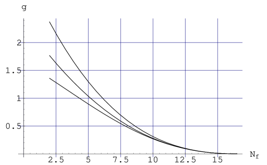
Figure 1: The critical exponent as a function of $N_{f}$: top: ${\cal O}(\epsilon^{3})$ order; middle: Padé; bottom: ${\cal O}(\epsilon^{4})$ order.

Note that in the obtained range of $N_{f}$ values ($4<N_{f}^{*}<6$), $\beta_{1}$ is still positive ($\beta_{1}$ changes sign for $N_{f}\simeq 8$) and of the same sign as $\beta_{0}$, so that the fixed point must arise from the contributions of higher then 2 loop beta function corrections, although I am assuming the Banks-Zaks expansion is still converging there. This is consistent with the fact (see section 7) that many QCD effective charges have negative 3-loop beta function coefficients in the above range.

7 Evidence for a negative UV fixed point in QCD

Can one substantiate the crucial assumption which underlines the previous derivation that no other sources of Landau singularities are present, but the one arising from the $\alpha>\alpha_{IR}$ region? Even barring complex (in $\alpha$ space) Landau singularities (such as complex poles in the beta function as in eq.(61) below), a potential problem can still arise from an eventual Landau singularity at $\alpha<0$, in the domain of attraction of the trivial IR fixed point $\alpha=0^{-}$. In this section I make the important additional assumption that perturbation theory is still asymptotic in the $\alpha<0$ region for the considered beta function. This implies that the corresponding coupling is itself free of renormalons ambiguities, despite their expected presence in generic conformal window amplitudes (see section 8). Otherwise one would have to consider ambiguities suppressing contributions (corresponding to power terms at short distances) which most probably would induce essential singularities at zero coupling and blow up exponentially as $\alpha\rightarrow 0^{-}$. An attractive candidate would be the “skeleton coupling” [15] associated to an hypothetical QCD “skeleton expansion”.

Given this assumption, at weak coupling the solution of the RG equation is controlled (even if $\alpha<0$) by the 2-loop beta function

$$\log(k^{2}/\Lambda^{2})={1\over\beta_{0}\alpha}+{\beta_{1}\over\beta_{0}^{2}}\log\alpha+const+....$$ (24)

where the $const$ is real. For $\alpha<0$ the right hand side of eq.(24) acquires a $\pm i\pi{\beta_{1}\over\beta_{0}^{2}}$ imaginary part, which implies the rays

$$k^{2}=|k^{2}|\exp\left(\pm i\pi{\beta_{1}\over\beta_{0}^{2}}\right)$$ (25)

map to the $\alpha<0$ region. Along the rays eq.(25), we are effectively in a QED like situation: increasing $|k^{2}|$, the coupling is either attracted to a non-trivial UV fixed point, or reaches a Landau singularity at some finite $|k^{2}|$. In the latter case, one must require that the condition:

$$|{\beta_{0}^{2}\over\beta_{1}}|<1$$ (26)

is satisfied in the whole $N_{f}$ range where eq.(14) is valid, which will confine the rays, hence the singularities to the second (or higher) sheet.

It turns out that in QCD condition eq.(26) can be satisfied only if $\beta_{1}<0$, and coincides with the 2-loop causality condition eq.(7), which requires $N_{f}>9.7$. Eq.(26) is however a necessary condition for causality for any beta function which admits a Landau singularity at negative $\alpha$ (in the domain of attraction of the $0^{-}$ trivial IR fixed point), and applies also if $\beta_{1}$ is positive in a general theory! Therefore, to preserve causality within the conformal window as determined by eq.(14), $\gamma$ should reach $1$ in the region $N_{f}>9.7$, which is clearly excluded (see Fig. 1). In order that eq.(14) be also a sufficient condition for causality one must thus check that a non-trivial (finite or infinite) UV fixed point $\alpha_{UV}$ is present at negative $\alpha$. A minimal example satisfying this requirement is the 3-loop beta function eq.(4) with $\beta_{0}>0$ and $\beta_{2}<0$ ($\beta_{1}$ can have any sign). Another example is provided by eq.(10).

It is worth mentioning eq.(26) is always violated [7] in the lower part of the conformal window in SQCD as determined by duality [8], and the previous argument thus implies the existence of a negative UV fixed point in this theory. In fact the “exact” NSVZ [16] beta function for $N_{f}=0$

$$\beta(\alpha)=-{\beta_{0}\alpha^{2}\over 1-{\beta_{1}\over\beta_{0}}\alpha}$$ (27)

does exhibit an (infinite) UV fixed point as $\alpha\rightarrow-\infty$, which might be the parent of a similar one present within Seiberg conformal window [8].

It is a priori possible in QCD to have an $\alpha<0$ Landau singularity rather then an $\alpha<0$ UV fixed point. A simple example (apart from the two-loop beta function eq.(6) with $\beta_{0}>0$ and $\beta_{1}<0$) is the three loop beta function eq.(4) with $\beta_{0},\beta_{2}>0$ and $\beta_{1}<0$, with a positive UV fixed point $\alpha_{UV}>\alpha_{IR}$ (one has to assume that the IR fixed point does not disappear before the $\alpha<0$ Landau singularity appears on the first sheet, i.e. the reverse situation to the one considered after eq.(4)). In such a case the bottom of the conformal window would be given as in the two-loop model by the condition $-\beta_{0}^{2}/\beta_{1}=1$, yielding $N_{f}^{*}\simeq 9.7$. Indeed, at such large $N_{f}$, any eventual Landau singularity from the $\alpha>\alpha_{IR}$ region has not yet reached the first sheet (as already observed) since $\gamma<0.4$ as shown by Fig. 1. This possibility is however disfavored as now explained.

A modified Banks-Zaks expansion: there is indeed some evidence that a negative UV fixed point is actually present in QCD. At the three-loop level, QCD effective charges associated to Euclidean correlators typically [11, 7] have $\beta_{2}<0$, and appear [7] to be causal and admit a negative UV fixed point, even somewhat below the two-loop causality boundary $N_{f}=9.7$ (in a range $7.0<N_{f}<9.7$). This evidence could be washed out in yet higher orders (e.g. the Padé improved three-loop beta functions [7]). However, additional and more systematic evidence for the existence of a couple of (positive-negative) IR-UV fixed points is provided by the following modified Banks-Zaks argument. Assume $\beta_{1}=0$, i.e. $N_{f}=8.05$. Then a real fixed point can still exist at the three-loop level if $\beta_{2}<0$, and actually one gets a pair of opposite signs zeroes at ${\tilde{\alpha}}=\pm(-\beta_{0}/\beta_{2})^{1/2}$, an IR and an UV fixed point. If $\beta_{0}$ is small enough, they are weakly coupled, and calculable through a modified Banks-Zaks expansion around $N_{f}=16.5$, applied to the auxiliary function ${\tilde{\beta}}(\alpha)\equiv\beta(\alpha)+\beta_{1}\alpha^{3}$ with the two-loop term removed. One gets

$${\tilde{\alpha}}_{IR,UV}=\pm{\tilde{\epsilon}}\left(1\mp{1\over 2}\ {\beta_{3,0}\over\beta_{2,0}}\ {\tilde{\epsilon}}+...\right)$$ (28)

where the expansion parameter ${\tilde{\epsilon}}\equiv(-\beta_{0}/\beta_{2,0})^{1/2}$, and $\beta_{i,0}$, the $N_{f}=16.5$ values of $\beta_{i}$ ($i=2,3$), are scheme dependent. Given a reference scheme whose beta function is known up to 4-loop (say, the $\overline{MS}$ scheme), $\beta_{2,0}$ can be obtained [17] from the $N_{f}=16.5$ value of the next-to-leading order coefficient in the expansion of the considered coupling in this scheme. Furthermore $\beta_{3,0}$ follows from the knowledge of the next-to-leading ($g_{1}=\beta_{1,1}=4.75$) and next-to-next-to-leading order ($g_{2}=-8.89$) coefficients in eq.(22) and the relation [6, 11] (which yields $g_{2}$ to start with when used [10] in the reference scheme, since the $g_{i}$’s are scheme invariant [6])

$${16\over 107}\ \beta_{3,0}+\left({16\over 107}\ \beta_{2,0}\right)^{2}=g_{1}^{2}-g_{2}\sim 31.4$$ (29)

For effective charges associated to Euclidean correlators, the correction in eq.(28) ranges from $0.1$ to $0.7$ at $N_{f}=8.05$ (where ${\tilde{\beta}}(\alpha)$ coincides with $\beta(\alpha)$), and gives some evidence for a couple of UV and IR fixed points around this value of $N_{f}$ (which is within the alleged conformal window, but below the 2-loop causality region). However, as far as the negative fixed point is concerned, this evidence is corroborated only if one assumes asymptoticity of perturbation theory at negative coupling for the considered beta functions. As pointed out above, this can hardly be expected for the beta functions of physical effective charges such as those associated to Euclidean correlators. The modified Banks-Zaks expansion should rather be applied to the aforementioned perturbative “skeleton coupling”, which may be free of renormalons and of the associated power terms. Assuming the correct “skeleton coupling” is the one identified [18, 19] through the “pinch technique”, one gets [15] $\beta_{2,0}=-17.5$ and eq.(29) yields $\beta_{3,0}=164.7$. Unfortunately, for these values the correction factor in eq.(28) is $1.34$ at $N_{f}=8.05$ and the expansion diverges! Nevertheless, these large corrections may indicate the necessity of resummation of the modified Banks-Zaks expansion rather then the absence of the fixed points. Some support for this interpretation is indicated by the satisfactory convergence of the standard (eq.(21)) Banks-Zaks expansion for the IR fixed point of the skeleton coupling

$$\alpha_{IR}=\epsilon+2.14\epsilon^{2}+...$$ (30)

which yields a next-to-leading order correction factor [6] of about $0.45$ at $N_{f}=8.05$ (for the Euclidean effective charges, the convergence is even better [10, 11, 7, 15]). It is also possible to investigate the existence of a negative UV fixed point at higher values of $N_{f}$ (where $\beta_{1}$ does not vanish), using a generalization of the modified Banks-Zaks expansion (see Appendix B). One finds slightly improved next-to-leading order corrections (of about $80\%$) at $N_{f}=11$. This makes the existence of a couple of (IR,UV) fixed points at least plausible around this value of $N_{f}$. However, below $N_{f}=9.7$, i.e. below the 2-loop causality region (where the negative UV fixed point is really needed), the corrections to the modified Banks-Zaks fixed point series are still over $100\%$.

Additional support is given by the calculation of the auxiliary critical exponent ${\tilde{\gamma}}\equiv d{\tilde{\beta}}(\alpha)/d\alpha|_{\alpha={\tilde{\alpha}_{IR}}}$, which gives

$${\tilde{\gamma}}=2\ \beta_{0}\ {\tilde{\epsilon}}(1+{\cal O}({\tilde{\epsilon}}^{2}))$$ (31)

(no ${\cal O}({\tilde{\epsilon}})$ correction!). For effective charges associated to Euclidean correlators one gets $0.6<{\tilde{\gamma}}<0.7$ at $N_{f}=8.05$ (where ${\tilde{\gamma}}$ coincides with $\gamma$), in reasonable agreement with the standard Banks-Zaks result (Fig. 1) $0.5<\gamma<0.6$. The agreement is again less satisfactory for the skeleton coupling, which yields ${\tilde{\gamma}}\sim 0.8$, but still qualitatively acceptable indicating the need for resummation.

It should be stressed that the non-trivial negative UV fixed point is actually not relevant to the proper analytic continuation of the coupling at complex $k^{2}$, which must be consistent [13] with (UV) asymptotic freedom. The latter condition ensures that eventual first sheet Landau singularities are localized within a bounded infrared region, as expected on physical grounds. This means that in presence of this fixed point, the correct analytic continuation must involve complex rather then negative values of $\alpha$ along the rays eq.(25), and one should approach the non-trivial (rather then the trivial) IR fixed point as $|k^{2}|\rightarrow 0$, and the trivial (rather then the non-trivial) UV fixed point as $|k^{2}|\rightarrow\infty$. This is possible since the solution of eq.(24) is not unique for a given (complex) $k^{2}$. For a similar reason, any eventual Landau singularity arising from the region $\alpha<\alpha_{UV}$, in the domain of attraction of the non-trivial UV fixed point, is not relevant to the correct analytic continuation. However, I have to assume that the considered beta function is such that all $\alpha>\alpha_{IR}$ singularities (and more generally all $|\alpha|=\infty$ singularities) are either irrelevant, or have the same phase $\pi/\gamma$ in $k^{2}$ plane, as in the example eq.(10).

On the other hand, it was implicitly assumed above that any $\alpha<0$ Landau singularity in the domain of attraction of the trivial $0^{-}$ IR fixed point is relevant, i.e. that the coupling will flow to the trivial $0^{+}$ UV fixed point once the $\alpha<0$ singularity is passed, even if there is another (positive) UV fixed point, as in the three loop example below eq.(27). Similarly, in presence of the negative UV fixed point, one has to assume that the coupling will still flow to the trivial UV fixed point (rather then the negative one), once the $\alpha>\alpha_{IR}$ Landau singularity is passed. This must be the case for consistency of the present approach, where causality violation in a coupling which satisfies UV asymptotic freedom is attributed either to the $\alpha<0$ or to the $\alpha>\alpha_{IR}$ Landau singularities.

8 “Perturbative” and “non-perturbative” components of condensates: the two loop APT coupling as a toy “non-perturbative” model

To illustrate the discussion in section 3, consider as a model for the full QCD amplitude $D(Q^{2})$ the standard “renormalon integral”

$$D(Q^{2})=\int_{0}^{Q^{2}}{dk^{2}\over k^{2}}\ \bar{\alpha}(k^{2})\ n\ \left({k^{2}\over Q^{2}}\right)^{n}$$ (32)

where the “non-perturbative” coupling $\bar{\alpha}(k^{2})$ (tentatively identified as a non-perturbative extension of the “skeleton coupling” [15], as suggested [20, 24] by the IR finite coupling approach [1] to power corrections) is IR finite and causal. I further assume the perturbative part $\alpha(k^{2})$ of the coupling is by itself IR finite even below the conformal window, but still differs there (where it is not causal) from the full non-perturbative coupling $\bar{\alpha}(k^{2})=\alpha(k^{2})+\delta\alpha(k^{2})$. Thus in this model eq.(3) holds, with

$$D_{\overline{PT}}(Q^{2})\equiv\int_{0}^{Q^{2}}{dk^{2}\over k^{2}}\ \alpha(k^{2})\ n\ \left({k^{2}\over Q^{2}}\right)^{n}$$ (33)

and

$$D_{\overline{NP}}(Q^{2})\equiv\int_{0}^{Q^{2}}{dk^{2}\over k^{2}}\ \delta\alpha(k^{2})\ n\ \left({k^{2}\over Q^{2}}\right)^{n}$$ (34)

One can show [21, 22] that $D_{\overline{PT}}(Q^{2})$ differs from the corresponding Borel sum $D_{PT}(Q^{2})$

$$D_{PT}(Q^{2})\equiv\int_{0}^{\infty}dz\exp\left(-z/\alpha(Q^{2})\right)\tilde{D}(z)$$ (35)

by a power correction

$$D_{\overline{PT}}(Q^{2})=D_{PT}(Q^{2})+[\tilde{C}_{PT}(-1)^{\delta}+C_{PT}]\left({\Lambda^{2}\over Q^{2}}\right)^{n}$$ (36)

where $\delta=n{\beta_{1}\over\beta_{0}^{2}}$ and $C_{PT}$ and $\tilde{C}_{PT}$ are real constants. $\tilde{C}_{PT}$ is the normalization of a complex component, which cancels the ambiguity of $D_{PT}(Q^{2})$ due to IR renormalons. Both $C_{PT}$ and $\tilde{C}_{PT}$ can in principle be determined [21, 22] from information contained in the (all-orders) perturbative series which build up $D_{PT}(Q^{2})$ (see also below and Appendix C). They represent the “perturbative” part of the condensate, the only one surviving within the conformal window. On the other hand, if $\delta\alpha(k^{2})$ decreases faster then ${\cal O}(1/k^{2n})$ at large $k^{2}$ (so that the leading power correction is of IR origin, i.e. the integral eq.(34) is not dominated by its UV tail), one gets for $Q^{2}\gg\Lambda^{2}$

$$D_{\overline{NP}}(Q^{2})\simeq C_{NP}\left({\Lambda^{2}\over Q^{2}}\right)^{n}+...$$ (37)

with

$$C_{NP}=\int_{0}^{\infty}{dk^{2}\over k^{2}}\ \delta\alpha(k^{2})\ n\ \left({k^{2}\over\Lambda^{2}}\right)^{n}$$ (38)

which represents the “genuine” non-perturbative part of the condensate, and should vanish within the conformal window. Thus for $Q^{2}\gg\Lambda^{2}$

$$D(Q^{2})\simeq D_{PT}(Q^{2})+C\left({\Lambda^{2}\over Q^{2}}\right)^{n}+...$$ (39)

with

$$C=\tilde{C}_{PT}(-1)^{\delta}+C_{PT}+C_{NP}$$ (40)

Let us now take the “APT coupling” $\alpha_{APT}(k^{2})$ as a toy model for the full non-perturbative coupling $\bar{\alpha}(k^{2})$ below the conformal window. It is defined [23] by the dispersion relation

$$\alpha_{APT}(k^{2})\equiv-\int_{0}^{\infty}{d\mu^{2}\over\mu^{2}+k^{2}}\ \rho(\mu^{2})$$ (41)

where the “spectral density”

$$\rho(\mu^{2})=\frac{1}{2\pi i}Disc\{\alpha(-\mu^{2})\}\equiv-\frac{1}{2\pi i}\{\alpha\left[-(\mu^{2}+i\epsilon)\right]-\alpha\left[-(\mu^{2}-i\epsilon)\right]\}$$ (42)

is proportional to the time-like discontinuity of the perturbative coupling $\alpha(k^{2})$. Eq.(41) implies in particular the absence of (first sheet) Landau singularities, and is therefore a “brute force” causal deformation of the perturbative coupling $\alpha(k^{2})$ (within the conformal window, where $\alpha(k^{2})$ is causal, it coincides with $\alpha_{APT}(k^{2})$ ). At large $k^{2}$, the discrepancy $\delta\alpha_{APT}(k^{2})$ between $\alpha_{APT}(k^{2})$ and $\alpha(k^{2})$ is an ${\cal O}(1/k^{2})$ power correction, and I therefore assume $0<n<1$ to guarantee the leading power correction is of IR origin. One then finds at large $Q^{2}$ that

$$D(Q^{2})\equiv D_{APT}(Q^{2})\simeq D_{PT}(Q^{2})+C_{APT}\left({\Lambda^{2}\over Q^{2}}\right)^{n}+...$$ (43)

where, assuming from now on that $\alpha(k^{2})$ is the two-loop coupling eq.(6), the Borel sum $D_{PT}(Q^{2})$ is given by [21, 22]

$$D_{PT}(Q^{2})=\int_{0}^{\infty}dz\exp\left(-z/\alpha(Q^{2})\right){\exp\left(-{\beta_{1}\over\beta_{0}}z\right)\over\left(1-{z\over z_{n}}\right)^{1+\delta}}$$ (44)

while for the power term one finds

$$C_{APT}=(-1)^{n}{\pi\over\sin\pi n}{z_{n}^{1+\delta}\over\Gamma(1+\delta)}$$ (45)

where $z_{n}=n/\beta_{0}$ and $\Lambda$ is defined from the solution of the two-loop renormalization group equation

$$\beta_{0}\log{Q^{2}\over\Lambda^{2}}={1\over\alpha}-{\beta_{1}\over\beta_{0}}\log\left({1\over\alpha}+{\beta_{1}\over\beta_{0}}\right)+{\beta_{1}\over\beta_{0}}$$ (46)

The result eq.(45) is obtained immediately from a similar one in [24], taking into account the different definition of $\Lambda$ used here (which is not the Landau singularity). This result actually assumes a space-like Landau singularity, i.e. that $\beta_{1}>0$, but eq.(45) makes also sense for $\beta_{1}<0$ where there is an IR fixed point, which suggests it might apply in this case as well, provided there are complex Landau singularities and causality is violated, i.e. for

$$0<-{\beta_{1}\over\beta_{0}^{2}}<1$$ (47)

Moreover when $\beta_{1}<0$ $D_{\overline{PT}}(Q^{2})$ (eq.(33)) is given by [21, 22]

$$D_{\overline{PT}}(Q^{2}) = \int_{0}^{z_{n}}dz\exp\left(-z/\alpha(Q^{2})\right){\exp\left(-{\beta_{1}\over\beta_{0}}z\right)\over\left(1-{z\over z_{n}}\right)^{1+\delta}}$$ (48)

$$= \int_{0}^{\infty}dz\exp\left(-z/\alpha(Q^{2})\right){\exp\left(-{\beta_{1}\over\beta_{0}}z\right)\over\left(1-{z\over z_{n}}\right)^{1+\delta}}-\int_{z_{n}}^{\infty}dz\exp\left(-z/\alpha(Q^{2})\right){\exp\left(-{\beta_{1}\over\beta_{0}}z\right)\over\left(1-{z\over z_{n}}\right)^{1+\delta}}$$

$$\equiv D_{PT}(Q^{2})+\tilde{C}_{PT}(-1)^{\delta}\left({\Lambda^{2}\over Q^{2}}\right)^{n}$$

which shows that in this 2-loop example the “perturbative part” of the power correction coincides with the “renormalon part”, i.e. we have in eq.(36)

$$C_{PT}=0$$ (49)

while [21, 22]

$$\tilde{C}_{PT}=-{\pi\over\sin\pi\delta}{z_{n}^{1+\delta}\over\Gamma(1+\delta)}$$ (50)

One can thus write eq.(45) in the form of eq.(40), i.e. we have $C_{APT}=\tilde{C}_{PT}(-1)^{\delta}+C_{PT}+C_{NP}$ with $\tilde{C}_{PT}$ and $C_{PT}$ as above, and one also finds

$$C_{NP}=\pi{z_{n}^{1+\delta}\over\Gamma(1+\delta)}\left({\cos\pi n\over\sin\pi n}+{\cos\pi\delta\over\sin\pi\delta}\right)$$ (51)

It is interesting to note that $C_{NP}$ vanishes when $\delta=-n$ (remember $0<n<1$), i.e. for ${\beta_{1}\over\beta_{0}^{2}}=-1$, which is the bottom of the conformal window in this model. This fact can be understood since there one might expect (in the 2-loop case) $\alpha_{APT}=\alpha$, which is an indication in favor of the correctness of eq.(45) when $\beta_{1}$ satisfies eq.(47). $C_{NP}$ does not however vanish identically within the conformal window, which means that $C_{NP}$ can be analytically continued from below to within the conformal window, but does not give the correct power correction there (see footnote 8).

9 A rationale for the infrared finite coupling approach to power corrections

The values of $N_{f}^{*}$ obtained in section 6 are substantially lower then the one following from the naive 2-loop causality condition ($N_{f}^{*}=9.7$) or the similar one from an earlier attempt based on “superconvergence” [7], and rather close to the number of light QCD flavors $N_{f}=3$ usually relevant for QCD phenomenology. As I now argue, this fact may give the underlying justification to the IR finite coupling approach [1] to power corrections. Indeed, the very notion that there is a non-perturbative modification $\delta\alpha$ of the coupling (section 8) may be only a convenient phenomenological parametrization of power corrections, without fundamental meaning. On the other hand, the existence of an IR finite coupling appears very natural within the conformal window, but there it is of entirely perturbative origin, with no need for a $\delta\alpha$ term. The following picture then suggests itself as an attractive alternative: in the decomposition eq.(3), only the “perturbative” conformal window amplitude $D_{\overline{PT}}$ may be related to the IR finite universal coupling (see e.g. eq.(33)), and there is no such thing as a non-perturbative modification of the coupling (a $\delta\alpha$ term). Still at large $Q^{2}$ one can write

$$D(Q^{2})\simeq D_{\overline{PT}}(Q^{2})+C_{NP}\left({\Lambda^{2}\over Q^{2}}\right)^{n}+...$$ (52)

with $C_{NP}$ now an independent parameter characterizing the “non-perturbative” vacuum, and bearing no connection (such as eq.(38)) to the universal coupling $\alpha$. The consecutive lost of predictive power following a priori from these more general assumptions is however compensated by the observation that $C_{NP}$ vanishes by definition for $N_{f}\geq N_{f}^{*}$, and can be expected to be still small for $N_{f}$ not too far below $N_{f}^{*}$, if the phase transition is “second order”, i.e. if $C_{NP}$ is continuous as a function of $N_{f}$, and vanishes as $N_{f}$ approaches $N_{f}^{*}$ from below (as in the 2-loop APT model of eq.(51)). It is thus at least plausible, given the low range $4<N_{f}^{*}<6$, that even at $N_{f}=3$ one can still neglect $C_{NP}$, i.e. that the main contribution to the condensate is given by its “perturbative” conformal window piece $\tilde{C}_{PT}(-1)^{\delta}+C_{PT}$ (see eq.(40)). An even more radical possibility would be that condensates are either entirely “perturbative” or “non-perturbative”, i.e. that $C_{NP}\equiv 0$ even below $N_{f}^{*}$ for those condensates which do not vanish within the conformal window. In such a case, the IR finite coupling approach would be justified at all $N_{f}$’s, independently of the value of $N_{f}^{*}$, as long as an IR fixed point is still present in the perturbative coupling.

This view raises the interesting possibility that the main contribution to the condensate may actually be calculable by perturbative means. To see this, recall [1] that power corrections can be parametrized in terms of low energy moments of the IR finite coupling. For instance in eq.(33) the low energy part below an IR cut-off $\mu_{I}$ yields a power correction $\lambda(\mu_{I})/Q^{2n}$ with $\lambda(\mu_{I})=\int_{0}^{\mu_{I}^{2}}{dk^{2}\over k^{2}}\ \alpha(k^{2})\ n\ k^{2n}$. As a first rough estimate (a more precise calculation shall be presented elsewhere [25]) one can replace $\alpha(k^{2})$ by $\alpha_{IR}$ in the expression for $\lambda(\mu_{I})$, and use the Banks-Zaks expansion eq.(30) to evaluate $\alpha_{IR}$ in the skeleton scheme (identified to the pinch technique coupling). In the range $4<N_{f}<6$ corresponding to the bottom of the conformal window one finds $0.41<\alpha_{IR}<0.52$, while at $N_{f}=3$ one finds $\alpha_{IR}=0.58$, with next to leading order corrections of the order 60-70% (I defined $\alpha\equiv\alpha_{s}/\pi$). These corrections, while substantial, do not completely rule out a perturbative approach. To get an hopefully more reliable estimate of $\alpha_{IR}$ at the bottom of the conformal window, one can indeed eliminate the Banks-Zaks parameter $\epsilon$ in eq.(22) in favor of $\alpha_{IR}$ using eq.(30) to obtain

$$\gamma={107\over 16}\alpha_{IR}^{2}(1+0.47\alpha_{IR}+...)$$ (53)

which seems to converge better. In leading order, one obtains $\gamma=1$ for $\alpha_{IR}=(16/107)^{1/2}\simeq 0.39$ (a scheme invariant prediction), whereas in next-to-leading order $\gamma=1$ is reached for $\alpha_{IR}\simeq 0.36$, with a small next-to-leading order correction of 0.17.

The possible relevance of conformal window physics and of the “perturbative” Banks-Zaks freezing of the coupling at low $N_{f}$ suggested here is very specific, and applies only to the calculation of “condensates” (already present within the conformal window) which appear in the short distance contributions to amplitudes. In particular, it is not assumed that the whole “non-perturbative” component $D_{\overline{NP}}(Q^{2})$ in eq.(3) is small for any $Q^{2}$: this is clearly not correct at $Q^{2}=0$ for the effective charge associated to the Adler D-function, whose exact value there is known from spontaneous chiral symmetry breaking arguments [26] and turns out to be negative, thus inconsistent with the positive result [10] following from the Banks-Zaks expansion at $N_{f}=3$. Thus the present suggestion differs from the related ideas in [10].

10 Behavior of the conformal window amplitudes in the $N_{f}\rightarrow-\infty$ “one-loop” limit

Although the arguments in section 5 require an IR fixed point in the perturbative coupling to be present only in some finite range $N_{f}^{c}<N_{f}<N_{f}^{*}$ below $N_{f}^{*}$, it is attractive to consider the possibility that the IR fixed point may actually persists down to the $N_{f}\rightarrow-\infty$ limit (where the “skeleton coupling” becomes [15] one loop). In such a case, the natural question arises whether the full conformal window amplitudes, which contain power terms, stay finite or blow up in this limit (despite the perturbative series coefficients and the corresponding Borel sum remaining themselves finite). That the latter can easily happen is demonstrated by the simplest 2-loop example eq.(50), which shows that $\tilde{C}_{PT}$ is singular for $\delta\rightarrow 0$, i.e. in the $\beta_{1}\rightarrow 0$ one-loop limit, while the Borel sum itself (eq.(44)) is finite. The singular behavior of $\tilde{C}_{PT}$ is actually a general fact. Indeed, the contribution of a dimension $2n$ operator in the OPE can always be parametrized [27] (assuming no anomalous dimension) as in eq.(39) and (40), where the $\tilde{C}_{PT}$ component is the “renormalon contribution” given by (minus) the singular part for $z\rightarrow z_{n}$ of the Borel transform

$$\tilde{C}_{PT}(-1)^{\delta}\left({\Lambda^{2}\over Q^{2}}\right)^{n} = \tilde{C}_{PT}\exp(-\delta)\exp\left(-z_{n}/\alpha(Q^{2})\right)(-\alpha(Q^{2}))^{-\delta}\left[1+{\cal O}(\alpha(Q^{2}))\right]$$ (54)

$$= -\int_{z_{n}}^{\infty}dz\exp\left(-z/\alpha(Q^{2})\right){K\over\left(1-{z\over z_{n}}\right)^{1+\delta}}\left[1+{\cal O}\left(1-{z\over z_{n}}\right)\right]$$

where $\delta=n{\beta_{1}\over\beta_{0}^{2}}$ (as below eq.(36)) and the factor $\exp(-\delta)$ is due to the definition of $\Lambda$ eq.(46). $K$ is the renormalon residue, related to $\tilde{C}_{PT}$ by

$$\tilde{C}_{PT}=-K\exp(\delta){\pi\over\sin\pi\delta}{z_{n}^{1+\delta}\over\Gamma(1+\delta)}$$ (55)

Note that eq.(55) reproduces eq.(50) for $K=\exp(-\delta)$, which is indeed the correct renormalon residue in this case (see eq.(44)). In the one-loop limit where $\beta_{1},\delta\rightarrow 0$, one finds the singular behavior (assuming $K$ remains finite as suggested by the behavior of the perturbative series coefficients)

$$\tilde{C}_{PT}\simeq-K{z_{n}\over\delta}=-K{\beta_{0}\over\beta_{1}}$$ (56)

It does not mean of course the full amplitude is singular, since there can be a cancellation between $\tilde{C}_{PT}(-1)^{\delta}$ and $C_{PT}+C_{NP}$ in eq.(40). The interesting question however is whether the perturbative ($\tilde{C}_{PT}(-1)^{\delta}+C_{PT}$) and non perturbative ($C_{NP}$) components of the condensate remain separately finite, i.e. the cancellation takes place between $\tilde{C}_{PT}$ and $C_{PT}$, or whether the cancellation (if any) takes place between the perturbative and the non perturbative pieces? If the perturbative condensate remains finite, eq.(36) and (44) become in the one-loop limit

$$D_{\overline{PT}}(Q^{2})=D_{PT}(Q^{2})+(const\pm i\pi z_{n})\left({\Lambda^{2}\over Q^{2}}\right)^{n}$$ (57)

with

$$D_{PT}(Q^{2})=\int_{0}^{\infty}dz\exp\left(-z/\alpha(Q^{2})\right){1\over 1-{z\over z_{n}}}$$ (58)

where the imaginary part in the power term removes the one-loop renormalon ambiguity in eq.(58).

Cancellation between the perturbative and non-perturbative components of the condensate occurs in the two-loop APT model of section 8, where $C_{PT}=0$ (and thus cannot cancel the divergent $\tilde{C}_{PT}$) while $C_{APT}$ is finite (see eq.(45)). On the other hand, in the three-loop case eq.(4) one finds (see Appendix C) that the perturbative part of the condensate remains finite by itself in the one-loop limit. The same is true for the more general beta function of eq.(10), which is conveniently written as

$$\beta(\alpha)=-\beta_{0}\alpha^{2}\ {1+(\omega+{\beta_{1}\over\beta_{0}})\alpha+{\lambda\over\beta_{0}}\alpha^{2}\over 1+\omega\alpha}$$ (59)

(this is a [2,1] “ Padé improved” 4-loop beta function, see [28]). More precisely, the statement is that, defining $D_{\overline{PT}}(Q^{2})$ as in eq.(33) with $\alpha(k^{2})$ obtained from the solution of the RG equation with the beta function eq.(59), the normalization $\tilde{C}_{PT}(-1)^{\delta}+C_{PT}$ of the power correction in eq.(36) remains finite in the limit $\beta_{1},\lambda\rightarrow 0$ with $\lambda/\beta_{1}$ and $\omega$ fixed (one of these constants may eventually be put to zero). This limit is taken at fixed ratios $\beta_{i}/\beta_{1}$ ($i\geq 1$), since one easily checks that $\omega=-\beta_{3}/\beta_{2}$ and $\lambda/\beta_{1}=\beta_{2}/\beta_{1}-\beta_{3}/\beta_{2}$. Note that cancellation occurs in the one-loop limit irrespective whether the IR fixed point tends to $+\infty$ (as in the three-loop case) or remains finite (as in the previous example) . Similar results hold for the [1,2] “ Padé improved” 4-loop beta function

$$\beta(\alpha)=-\beta_{0}\alpha^{2}\ {1+(\tilde{\omega}+{\beta_{1}\over\beta_{0}})\alpha\over 1+\tilde{\omega}\alpha+{\tilde{\lambda}\over\beta_{0}}\alpha^{2}}$$ (60)

in the limit $\beta_{1},\tilde{\lambda}\rightarrow 0$ with $\tilde{\lambda}/\beta_{1}$ and $\tilde{\omega}$ fixed. On the other hand, one finds no cancellation takes place in the similar limit $\beta_{1},\beta_{2}\rightarrow 0$ with $\beta_{2}/\beta_{1}$ fixed if one sets $\tilde{\omega}=0$ in eq.(60), which gives

$$\beta(\alpha)=-\beta_{0}\alpha^{2}\ {1+{\beta_{1}\over\beta_{0}}\alpha\over 1-{\beta_{2}\over\beta_{0}}\alpha^{2}}$$ (61)

However in this example higher order beta function coefficients are further suppressed in the one loop limit compared to $\beta_{1}$ and $\beta_{2}$. Although the ultimate reason for presence or absence of cancellation is not clear to the author, the previous examples do suggest that cancellation may be a generic feature, which requires no fine-tuning of parameters if the one-loop limit is taken at fixed and finite ratios $\beta_{i+1}/\beta_{i}$ ($i\geq 1$), as follows in QCD from large $N_{f}$ counting rules for the class of beta functions which become one-loop at large $N_{f}$ (I assume the limit is taken at fixed $\alpha$, which means $\alpha$ contains an extra factor of $N_{f}$ compared to the standard normalization).

11 Conclusions

1) Landau singularities are usually interpreted as the signal from the perturbative side of the occurrence of non-perturbative phenomena. However, in the usual picture at fixed $N_{f}$, this interpretation is obscured by the fact that they appear as technical artifacts of perturbation theory, and would never show up in the full non-perturbative amplitude. In contrast to this, the previous considerations give a more direct, physical motivation for Landau singularities, assuming a two-phase structure of QCD: they should trace the lower boundary $N_{f}^{*}$ of the conformal window. This approach avoids the notoriously tricky disentangling between the “perturbative” and the “non-perturbative” parts of the QCD amplitudes within the conformal window, since they are by definition entirely “perturbative” there. On the other hand, such a separation is naturally achieved below the conformal window, by introducing the analytic continuation of the conformal window amplitudes to the $N_{f}<N_{f}^{*}$ region. This procedure has been illustrated using the “APT” model as a toy “non-perturbative” model for the coupling below $N_{f}^{*}$. If these ideas are correct, they reveal a deep connection between information of essentially “perturbative” origin (the onset of Landau singularities on the first sheet) and “non-perturbative” phenomena (the emergence of a new phase of QCD when $N_{f}$ is varied).

When extended to SQCD, these considerations suggest that the NSVZ beta function eq.(27), which has a pole at positive coupling corresponding to a space-like IR Landau singularity, cannot really be “non-perturbatively exact”, despite it receives no contribution from the instanton sector. Instead, the Landau singularity must be present as a signal (from the “perturbative” side) that below Seiberg conformal window [8] there are other more “genuine” non-perturbative contributions, unrelated to instantons, which remove the singularity (the point that instantons do not exhaust all non-perturbative phenomena is familiar in QCD). Note the present view differs from the one expressed in [29].

2) Assuming that the perturbative QCD coupling has a non-trivial IR fixed point $\alpha_{IR}$ even in some range below $N_{f}^{*}$ leads to the equation $\gamma(N_{f}=N_{f}^{*})=1$ to determine $N_{f}^{*}$ from the critical exponent $\gamma$ at the IR fixed point. Using the available terms in the Banks-Zaks expansion, this equation yields $4\leq N_{f}^{*}\leq 6$. It would clearly be desirable to have more terms to better control the accuracy of the Banks-Zaks expansion. Note that this condition is inconsistent with the existence of an analogue of Seiberg duality in QCD, which would rather imply $\gamma(N_{f}=N_{f}^{*})=0$.

3) The low value obtained for $N_{f}^{*}$, and its closeness to $N_{f}=3$, gives some justification to the IR finite coupling approach to power corrections, and its associated “universality” property: the latter could be violated only by “genuine non-perturbative terms” (unrelated to the IR finite coupling or to an hypothetical non-perturbative modification thereof which may very well not exist) which vanish within the conformal window and may be expected to be still small for values such as $N_{f}=3$ which are not too far below $N_{f}^{*}$. Thus in a first approximation the bulk of those power corrections whose very existence is not linked to the non-trivial vacuum below $N_{f}^{*}$ (condensates which do not break any symmetry of the vacuum, like the gluon condensate) should be given by the “perturbative” part of the condensate contained in the conformal window amplitude $D_{\overline{PT}}(Q^{2})$, and related to the perturbative IR finite QCD coupling. Consequently, their normalization could even be calculable from perturbative input: indeed one obtains $\alpha_{IR}\simeq 0.4$ at the bottom of the conformal window. In this way, the physics of the conformal window becomes relevant to real-world QCD with $N_{f}=3$ flavors.

4) Some conditions on the QCD beta function are required: the only source of Landau singularities must arise from the $\alpha>\alpha_{IR}$ region. One needs in particular a negative UV fixed point $\alpha_{UV}$ if perturbation theory is still asymptotic at negative coupling for the considered beta function. There is indeed some tentative evidence (relying on a modified Banks-Zaks expansion) for such a fixed point in QCD. However, the asymptoticity of perturbation theory at negative coupling, which points out to a very specific coupling, remains to be understood. An attractive possibility is to identify this coupling to the “skeleton coupling” [15] associated to a (yet hypothetical) QCD “skeleton expansion”.

5) A negative UV fixed point is also required in the SQCD case, where duality fixes the conformal window.

6) The condition $0<\gamma<1$ appears to be necessary [7] for causality under rather general assumptions. A similar constraint involving the UV fixed point critical exponent has been derived [14] using completely different arguments as a consistency condition for non-asymptotically free supersymmetric gauge theories to have a non-trivial physical (positive) UV fixed point.

7) It is possible the IR fixed point persists in the perturbative QCD coupling down to the $N_{f}\rightarrow-\infty$ one-loop limit. It may even remain finite in this limit: a simple example is provided by the beta function eq.(10) with one positive pole $\alpha_{P}$ (the required Landau singularity) and two opposite sign zeroes $\alpha_{IR}$ and $\alpha_{UV}$. The one-loop limit is achieved for $\alpha_{IR}=\alpha_{P}$ and $\alpha_{UV}=-\infty$. In this example, although $\alpha_{IR}$ remains finite, $\gamma$ tends to $+\infty$, and therefore necessarily crosses $1$ and violates causality before the one-loop limit is reached, as expected.

8) The behavior of conformal window amplitudes (which contain power contributions) has been studied in various examples where the IR fixed point is present up to the one-loop limit. The results indicate that, beyond 2-loop, finiteness of the full amplitudes in this limit may be a natural and generic feature requiring no fine tuning (as suggested by the behavior of the corresponding perturbative series), provided the limit is taken at fixed and finite ratios of the perturbative beta function coefficients beyond one-loop: this is indeed the case for beta functions (such as the one associated to the “skeleton coupling”) which become one-loop in the $N_{f}\rightarrow-\infty$ limit of QCD.

Appendix A A necessary condition for causality

Let us show that the condition eq.(14)

$$0<\gamma<1$$ (62)

is a necessary one for causality. The case where there is an $\alpha>\alpha_{IR}$ Landau singularity was dealt with in section 5. Let us now consider the alternative situation where there is an $\alpha>\alpha_{IR}$ UV fixed point. Then along the ray eq.(17) there is an “irrelevant” real trajectory where the coupling flows from the non-trivial IR fixed point to the non-trivial UV fixed point. This trajectory is “irrelevant” since the correct relevant analytic continuation of the coupling to the complex momentum plane must always respect the condition of UV asymptotic freedom. This is possible since the solution of the RG equation along a given ray is not unique, and there can be another (complex) solution along the same ray, which approaches the trivial UV fixed point. The crucial point however is that this alternative solution cannot approach the non-trivial IR fixed point at low momenta, since the solution along a given ray in the domain of attraction of a given non-trivial fixed point is instead unique (unless one reaches a Landau singularity), as will be shown below. Consequently, the “relevant” solution along the ray eq.(17) which respects UV asymptotic freedom must in the infrared approach the trivial $0^{-}$ IR fixed point. Since the relevant solution along the space-like axis approaches instead the non-trivial IR fixed point, this means that there must be a curve in the complex $k^{2}$ plane (a “separatrix”) which separates the region which is in the domain of attraction of the non-trivial IR fixed point from the one which is in the domain of attraction of the trivial IR fixed point. If the condition eq.(62) is violated, the ray eq.(17), hence also the separatrix, belong to the first sheet. I shall assume that such an infrared separatrix (for instance a ray between the space-like axis and the ray eq.(17)) also indicates a discontinuity at finite $k^{2}$, hence the presence of a Landau singularity on the first sheet along the separatrix. In the 3-loop example of eq.(4) with $\beta_{0}>0$, $\beta_{2}>0$ and $\beta_{1}<0$, this singularity is the $\alpha<0$ Landau singularity along the ray eq.(25), whose phase $\pi|\beta_{1}|/\beta_{0}^{2}$ is indeed intermediate [7] in this case between zero (the space-like axis) and the phase $\pi/\gamma$ of the ray eq.(17).

To prove unicity of the solution of the renormalization group equation along a given ray, under the constraint this solution approaches a given non-trivial IR fixed point in the infrared, consider the solution eq.(19) of this equation around $\alpha=\alpha_{IR}$. Inverting to solve for $\alpha_{IR}-\alpha$ yields the unique power series solution (with $(k^{2}/\Lambda^{2})^{\gamma}$ as expansion parameter)

$$\alpha_{IR}-\alpha=\left({k^{2}\over\Lambda^{2}}\right)^{\gamma}-{\gamma_{1}\over\gamma}\left({k^{2}\over\Lambda^{2}}\right)^{2{\gamma}}+...$$ (63)

which suggests that there is a unique solution, at least in a neighborhood of $k^{2}=0$.

Note the corresponding unicity for the expansion around a trivial fixed point does not hold. Consider the weak coupling solution eq.(24) of the RG equation. One finds that there are a priori two possible solutions which approach the trivial IR fixed point $0^{-}$, i.e. such that $|\alpha(k^{2})|\rightarrow 0$ for $k^{2}\rightarrow 0$, along the rays $k^{2}=|k^{2}|\exp(\pm i\pi\beta_{1}/\beta_{0}^{2})$. Putting $\alpha\equiv|\alpha|\exp(i\phi)$, one solution corresponds to $\alpha<0$, i.e. $\phi\equiv\pm\pi$, while the other gives complex values of $\alpha$, i.e. $\phi\equiv\phi(k^{2})\neq 0,\pm\pi$ with $\phi(k^{2})\rightarrow\pm\pi$ (and $\sin(\phi)/|\alpha|\rightarrow\pm 2\pi\beta_{1}/\beta_{0}$) for $k^{2}\rightarrow 0$. Indeed the real part of eq.(24) yields

$$\log|{k^{2}\over\Lambda^{2}}|={1\over\beta_{0}|\alpha|}\cos\phi+...$$ (64)

while the imaginary part yields

$$\pm\pi{\beta_{1}\over\beta_{0}^{2}}=-{1\over\beta_{0}|\alpha|}\sin\phi+{\beta_{1}\over\beta_{0}^{2}}\phi+...$$ (65)

from which the previous results follow. Eventually we also have $\phi(k^{2})\rightarrow 0$ for $k^{2}\rightarrow\infty$ so that $\alpha(k^{2})$ approaches the trivial UV fixed point $0^{+}$ if this possible “relevant” solution is actually realized, as in the standard two-loop case with $\beta_{1}/\beta_{0}>0$ (where the $\alpha<0$ solution is attracted towards the non-trivial (negative) UV fixed point, and is therefore “irrelevant”). A similar situation arises in the 3-loop case of eq.(4) with $\beta_{0}>0$, $\beta_{2}<0$ and $\beta_{1}>0$ and large enough so that the phase $\pi/\gamma$ of the ray eq.(17) is intermediate between zero and the phase $\pi\beta_{1}/\beta_{0}^{2}$ of the ray eq.(25).

Appendix B A modified Banks-Zaks expansion

One introduces the auxiliary beta function

$${\tilde{\beta}}(\alpha)\equiv-\beta_{0}\alpha^{2}-{\tilde{\beta}_{1}}\alpha^{3}-\beta_{2}\alpha^{4}-\beta_{3}\alpha^{5}+...$$ (66)

where the two-loop coefficient is replaced by ${\tilde{\beta}_{1}}\equiv\rho\beta_{0}$ where $\rho$ is an arbitrary constant, and solves perturbatively the equation ${\tilde{\beta}}(\alpha)=0$ for $\beta_{0}\rightarrow 0$, i.e. $N_{f}\rightarrow 16.5$ at fixed $\rho$. Then for each value of $N_{f}$, one adjusts $\rho$ in the resulting series to the value $\rho=\beta_{1}/\beta_{0}$ for which ${\tilde{\beta}}(\alpha)$ coincides with the true beta function $\beta(\alpha)$. This procedure yields the modified Banks-Zaks series for a couple of (IR,UV) fixed points

$${\tilde{\alpha}}_{IR,UV}=\pm{\tilde{\epsilon}}+{1\over 2}\left(\rho-{\beta_{3,0}\over\beta_{2,0}}\right){\tilde{\epsilon}}^{2}+...$$ (67)

with ${\tilde{\epsilon}}\equiv(-\beta_{0}/\beta_{2,0})^{1/2}$. For the auxiliary critical exponent

$${\tilde{\gamma}}\equiv d{\tilde{\beta}}(\alpha)/d\alpha|_{\alpha={\tilde{\alpha}_{IR}}}$$ (68)

one gets the expansion

$${\tilde{\gamma}}=2\ \beta_{0}\ {\tilde{\epsilon}}(1+\rho{\tilde{\epsilon}}+...)$$ (69)

For $\rho=0$ (which corresponds to $N_{f}=8.05$) one recovers the results of section 7, while for $\rho=-2.55$ (which corresponds to $N_{f}=11$) one gets a next-to leading order correction of about $80\%$ in eq.(67) and of $60\%$ in eq.(69) if one uses the pinch technique “skeleton coupling”. Going to even larger $N_{f}$ values will presumably not help: although the next-to-leading order correction in the fixed point series decreases (due to a cancellation between $\rho$ and $-\beta_{3,0}/\beta_{2,0}$), it increases in the critical exponent series due to the larger value of $\rho$, conveying the suspicion that still higher order corrections in eq.(67) will be large (as they must since one does not expect the negative UV fixed point, at the difference of the IR fixed point, to approach zero as $\beta_{0}\rightarrow 0$).

Appendix C Power corrections from IR finite perturbative coupling

I first recall the results of [21, 22] to compute the power correction in eq.(36) when the perturbative coupling $\alpha(k^{2})$ in eq.(33) has a non-trivial IR fixed point. The main observation is that $D_{\overline{PT}}(Q^{2})$ remains finite (and approaches $\alpha_{IR}$) for $Q^{2}\rightarrow 0$. Eq.(36) then implies that in the same limit the Borel sum eq.(35) diverges as

$$D_{PT}(Q^{2})\sim-[\tilde{C}_{PT}(-1)^{\delta}+C_{PT}]\left({\Lambda^{2}\over Q^{2}}\right)^{n}$$ (70)

This behavior can be reproduced with the following ansatz for the Borel image $\tilde{D}(z)$ of $D_{PT}(Q^{2})$ . Put

$$\tilde{D}(z)\equiv\exp\left({z\over\alpha_{IR}}\right)F(z)$$ (71)

and assume

$$F(z)\sim{\kappa\over z^{a}}$$ (72)

as $z\rightarrow+\infty$ (with $a<1$). Then eq.(35) implies, since the integral is dominated by the large $z$ contribution for $Q^{2}\rightarrow 0$

$$D_{PT}(Q^{2})\sim\kappa\int_{0}^{\infty}dz\exp\left(-z/A(Q^{2})\right){1\over z^{a}}=\kappa\ \Gamma(1-a)A(Q^{2})^{1-a}$$ (73)

where

$${1\over A(Q^{2})}\equiv{1\over\alpha(Q^{2})}-{1\over\alpha_{IR}}$$ (74)

In the IR limit we get from eq.(16) that

$$A(Q^{2})\sim\left({\Lambda^{2}\over Q^{2}}\right)^{\gamma}$$ (75)

(the normalization implies a proper redefinition of $\Lambda$), hence

$$D_{PT}(Q^{2})\sim\kappa\ \Gamma(1-a)\left({\Lambda^{2}\over Q^{2}}\right)^{\gamma(1-a)}$$ (76)

Comparing with eq.(70), eq.(76) determines

$$\tilde{C}_{PT}(-1)^{\delta}+C_{PT}=-\kappa\ \Gamma(1-a)$$ (77)

from the $z\rightarrow+\infty$ behavior of $\tilde{D}(z)$, and reveals that

$$n=\gamma\ (1-a)$$ (78)

To determine the normalization constant $\kappa$ in eq.(72), one uses the fact that $D_{\overline{PT}}(Q^{2})$ as well as $D_{PT}(Q^{2})$ satisfy the differential equation [22]

$$D(\alpha)+{1\over n}\beta(\alpha){dD\over d\alpha}=\alpha$$ (79)

where $\alpha\equiv\alpha(Q^{2})$, which yields an integral equation for $\tilde{D}(z)$

$$\int_{0}^{\infty}dz\exp\left(-z/\alpha\right)\tilde{D}(z)+{1\over n}{\beta(\alpha)\over\alpha^{2}}\int_{0}^{\infty}dz\exp\left(-z/\alpha\right)z\tilde{D}(z)=\alpha$$ (80)

Introducing the Borel representation of ${\beta(\alpha)\over\alpha^{2}}$, one can get an equation [21] involving only Borel space functions.

Let us apply this method to the [2,1] “Padé improved” 4-loop beta function $\beta(\alpha)=-\beta_{0}\alpha^{2}\ {1+(\omega+{\beta_{1}\over\beta_{0}})\alpha+{\lambda\over\beta_{0}}\alpha^{2}\over 1+\omega\alpha}$ of eq.(59). Multiplying both sides of eq.(80) by the beta function denominator $1+\omega\alpha$, one gets

$$(1+\omega\alpha)\int_{0}^{\infty}dz\exp\left(-z/\alpha\right)\tilde{D}(z)-{1\over z_{n}}\left[1+\left(\omega+{\beta_{1}\over\beta_{0}}\right)\alpha+{\lambda\over\beta_{0}}\alpha^{2}\right]\int_{0}^{\infty}dz\exp\left(-z/\alpha\right)z\tilde{D}(z)$$

$$=\alpha(1+\omega\alpha)$$ (81)

where $z_{n}={n\over\beta_{0}}$. Using the convolution multiplication theorem for Borel transforms eq.(81) becomes in Borel space

$$\tilde{D}(z)+\omega\int_{0}^{z}dy\tilde{D}(y)-{1\over z_{n}}\left[z\tilde{D}(z)+\left(\omega+{\beta_{1}\over\beta_{0}}\right)\int_{0}^{z}dy\ y\tilde{D}(y)+{\lambda\over\beta_{0}}\int_{0}^{z}dy(z-y)y\tilde{D}(y)\right]$$

$$=1+\omega z$$ (82)

After taking two derivatives with respect to $z$, eq.(82) yields the homogenous second order differential equation with linear coefficients

$$\left(1-{z\over z_{n}}\right)\tilde{D}^{{}^{\prime\prime}}(z)-\left[{2\over z_{n}}-\omega+\left(\omega+{\beta_{1}\over\beta_{0}}\right){z\over z_{n}}\right]\tilde{D}^{{}^{\prime}}(z)-\left[{1\over z_{n}}\left(\omega+{\beta_{1}\over\beta_{0}}\right)+{\lambda\over\beta_{0}}{z\over z_{n}}\right]\tilde{D}(z)=0$$ (83)

which is equivalent to eq.(81) with the boundary conditions

$$\tilde{D}(0) = 1$$

$$\tilde{D}^{{}^{\prime}}(0) = {1\over z_{n}}$$

This equation can be solved in a standard way [30] in term of confluent hypergeometric functions. If one writes $\tilde{D}(z)$ as in eq.(71), then $F(z)\equiv F(a,c;x)$, a solution of the confluent hypergeometric equation

$$x{d^{2}F\over dx^{2}}+(c-x){dF\over dx}-aF=0$$ (85)

where

$$x=x_{0}\left(1-{z\over z_{n}}\right)$$ (86)

with

$$x_{0}=({1\over\alpha_{IR}}-{1\over\alpha_{UV}})z_{n}$$ (87)

and $\alpha_{IR}$ and $\alpha_{UV}$ are the positive and negative zeroes of the beta function eq.(59). Moreover we have

$$c=2+{\beta_{1}\over\beta_{0}}z_{n}\equiv 2+\delta$$ (88)

whereas the parameter $a$ is related to the IR fixed point critical exponent $\gamma$ by eq.(78). In term of $F(a,c;x)$, the boundary conditions eq.(LABEL:eq:bound-cond) read

$$F(a,c;x_{0}) = 1$$

$$x_{0}{dF\over dx}|_{x=x_{0}} = {z_{n}\over\alpha_{IR}}-1$$

The general solution of eq.(85) is

$$F(a,c;x)=F_{sing}(a,c;x)+F_{reg}(a,c;x)$$ (90)

where in standard notation [30]

$$F_{reg}(a,c;x)=K_{r}\ \Phi(a,c;x)\equiv K_{r}\ \Phi(a,2+\delta;x)$$ (91)

and

$$F_{sing}(a,c;x)=K_{s}\ x^{1-c}\ \Phi(a-c+1,2-c;x)\equiv K_{s}\ \left({1\over x}\right)^{1+\delta}\ \Phi(a-1-\delta,-\delta;x)$$ (92)

where $K_{r}$ and $K_{s}$ are integration constants to be determined from eq.(LABEL:eq:bound-cond1). To find $\kappa$ in eq.(72), one needs the $z\rightarrow+\infty$ behavior, which corresponds (eq.(86)) to $x\rightarrow-\infty$, since $x_{0}>0$. One gets [30] in this limit

$$F_{sing}(a,c;x)\sim\kappa_{s}\ {1\over z^{a}}$$ (93)

with

$$\kappa_{s}=K_{s}\ {\Gamma(-\delta)\over\Gamma(1-a)}(-1)^{1+\delta}\left({z_{n}\over x_{0}}\right)^{a}$$ (94)

and

$$F_{reg}(a,c;x)\sim\kappa_{r}\ {1\over z^{a}}$$ (95)

with

$$\kappa_{r}=K_{r}\ {\Gamma(2+\delta)\over\Gamma(2+\delta-a)}\left({z_{n}\over x_{0}}\right)^{a}$$ (96)

Note that $\kappa_{s}$ is complex, corresponding to the “renormalon contribution”. Since

$$\kappa=\kappa_{r}+\kappa_{s}$$ (97)

one obtains comparing with eq.(77)

$$\tilde{C}_{PT}=K_{s}\left({z_{n}\over x_{0}}\right)^{a}\Gamma(-\delta)$$ (98)

and

$$C_{PT}=-K_{r}\left({z_{n}\over x_{0}}\right)^{a}{\Gamma(2+\delta)\over\Gamma(2+\delta-a)}\Gamma(1-a)$$ (99)

Thus the normalization of the “condensate” in this model is

$$\tilde{C}_{PT}(-1)^{\delta}+C_{PT}=\left({z_{n}\over x_{0}}\right)^{a}\left[(-1)^{\delta}K_{s}\ \Gamma(-\delta)-K_{r}\ {\Gamma(2+\delta)\over\Gamma(2+\delta-a)}\Gamma(1-a)\right]$$ (100)

with $K_{r},K_{s}$ determined by eq.(LABEL:eq:bound-cond1) as mentioned above. Using the relation ${d\Phi(a,c;x)\over dx}={a\over c}\Phi(a+1,c+1;x)$, this equation yields

$$K_{s}\left({1\over x_{0}}\right)^{1+\delta}\Phi(a-1-\delta,-\delta;x_{0})+K_{r}\ \Phi(a,2+\delta;x_{0}) = 1$$

$$K_{s}\left[(-1-\delta)\left({1\over x_{0}}\right)^{1+\delta}\Phi(a-1-\delta,-\delta;x_{0})+\left({1\over x_{0}}\right)^{\delta}\left({a-1-\delta\over-\delta}\right)\Phi(a-\delta,1-\delta;x_{0})\right] +$$

$$K_{r}\ {a\over 2+\delta}\ x_{0}\ \Phi(a+1,3+\delta;x_{0}) = {z_{n}\over\alpha_{IR}}-1$$

Consider now the one-loop limit where $\beta_{1}$ and $\lambda\rightarrow 0$ with $\omega$ and $\lambda/\beta_{1}$ fixed. This limit corresponds to fixed ratios $\beta_{i}/\beta_{1}$ ($i>1$), for instance we have

$${\beta_{2}\over\beta_{0}} = -\omega(1-r){\beta_{1}\over\beta_{0}}$$

$${\beta_{3}\over\beta_{0}} = \omega^{2}(1-r){\beta_{1}\over\beta_{0}}$$

where $r\equiv{\lambda\over\beta_{1}}{1\over\omega}$ (note that $\omega=-\beta_{3}/\beta_{2}$). In this limit $\gamma\rightarrow+\infty$, hence (eq.(78)) $a\rightarrow 1$, $\delta\rightarrow 0$, while $x_{0}\sim{z_{n}\over\alpha_{IR}}\sim-z_{n}\omega$ remains finite (I assume presently $\omega<0$ and $\neq 0$ to have the beta function pole positive, finite). Moreover a little algebra shows that ${a-1-\delta\over-\delta}\sim-{\lambda\over\beta_{1}}\alpha_{IR}\sim r$ is finite. This implies, using the small x expansion of $\Phi(a,c;x)$, that $\Phi(a-1-\delta,-\delta;x_{0})\sim 1+r(e^{x_{0}}-1)$. Using also the special values [30] of the $\Phi$ function, the system eq.(LABEL:eq:bound-cond2) then simplifies to

$$K_{s}\ {1\over x_{0}}\left[1+r(e^{x_{0}}-1)\right]-K_{r}\ {1\over x_{0}}(1-e^{x_{0}}) \sim 1$$

$$K_{s}\left[-{1\over x_{0}}\left(1+r(e^{x_{0}}-1)\right)+re^{x_{0}}\right]+K_{r}\ {1\over x_{0}}\left[1-e^{x_{0}}(1-x_{0})\right] \sim x_{0}-1$$

which gives the one-loop limit values

$$K_{s} \sim x_{0}e^{-x_{0}}$$

$$K_{r} \sim (1-r)x_{0}e^{-x_{0}}$$

Finally in this limit eq.(100) yields

$$\tilde{C}_{PT}(-1)^{\delta}+C_{PT} \sim \left({z_{n}\over x_{0}}\right)^{a}\left(-{K_{s}\over\delta}-{K_{r}\over 1-a}\right)$$

$$\sim -z_{n}\ e^{-x_{0}}\left({1\over\delta}+{1-r\over 1-a}\right)$$

where the two separately divergent terms in eq.(LABEL:eq:condensate-limit) cancel in leading order as a consequence of the previously mentioned relation ${a-1-\delta\over-\delta}\sim r$, leaving a finite one-loop limit. Note that $\tilde{C}_{PT}$ diverges as

$$\tilde{C}_{PT}\sim-{\beta_{0}\over\beta_{1}}e^{-x_{0}}$$ (106)

in agreement with the general expectation eq.(56). Note also we should have $r>1$ if $\beta_{1}>0$ or $r<0$ if $\beta_{1}<0$ in order that $\alpha_{UV}<0<\alpha_{IR}<\alpha_{P}$ (the case $0<r<1$ is also possible if $\beta_{1}<0$, and corresponds to a situation where $\alpha_{P}<\alpha_{UV}<0<\alpha_{IR}$).

The case where $\omega=0$ ($r=\infty$) corresponds to the standard three-loop beta function eq.(4), and has to be treated separately. Here too, one finds that cancellation occurs generically, provided the one loop limit is taken at fixed and finite ratio $\beta_{2}/\beta_{1}$ (there is no cancellation if $\beta_{1}\equiv 0$). Then a little algebra shows that $a\rightarrow 1$ and $\delta\rightarrow 0$ as before, while this time $x_{0}\sim 2{z_{n}\over\alpha_{IR}}\rightarrow 0$. Moreover one finds that $\left({a-1-\delta\over-\delta}\right)x_{0}\sim-{\beta_{2}\over\beta_{1}}z_{n}$ is finite. The system eq.(LABEL:eq:bound-cond2) simplifies in this limit to

$$K_{s}\ {1\over x_{0}}\left(1-{\beta_{2}\over\beta_{1}}z_{n}\right)+K_{r} \sim 1$$

$$K_{s}\left[-{1\over x_{0}}\left(1-{\beta_{2}\over\beta_{1}}z_{n}\right)+{\beta_{0}\over 2\beta_{1}\alpha_{IR}}\right]+{1\over 2}x_{0}\ K_{r} \sim -1$$

which gives, using $x_{0}\sim 2{z_{n}\over\alpha_{IR}}\rightarrow 0$ and $\alpha_{IR}^{2}\sim-{\beta_{0}\over\beta_{2}}$ (one must take $\beta_{2}<0$ to have an IR fixed point present down to the one-loop limit)

$$K_{s}\ {1\over x_{0}}\left(1-{\beta_{2}\over\beta_{1}}z_{n}\right)+K_{r} \sim 1$$

$$-K_{s}\ {1\over x_{0}}+{1\over 2}x_{0}\ K_{r} \sim -1$$

and yields

$$K_{s} \sim x_{0}\rightarrow 0$$

$$K_{r} \sim {\beta_{2}\over\beta_{1}}z_{n}$$

From eq.(98) and (99) one then gets after a little algebra the values

$$\tilde{C}_{PT}\sim-{\beta_{0}\over\beta_{1}}$$ (110)

and

$$C_{PT}\sim{\beta_{0}\over\beta_{1}}$$ (111)

which again do cancel in leading order, leaving a finite one-loop limit condensate.

References

- [1] See e.g. Yu.L. Dokshitzer, in International Conference “Frontiers of Matter”, Blois, France, June 1999 [hep-ph/9911299].
- [2] G. Grunberg, hep-ph/0009272.
- [3] G. Grunberg, Phys.Lett. B349 (1995) 469.
- [4] T. Banks and A. Zaks, Nucl. Phys. B196 (1982) 189.
- [5] A.R. White, Phys.Rev. D29 (1984) 1435; Int. J. Mod. Phys. A8 (1993) 4755 [hep-th/9303053].
- [6] G. Grunberg, Phys.Rev. D46 (1992) 2228.
- [7] E. Gardi and G. Grunberg, JHEP 03 (1999) 024 [hep-th/9810192].
- [8] N. Seiberg, Nucl. Phys. B435 129 (1995) [hep-th/9411149].
- [9] D. Anselmi, private communication.
- [10] P.M. Stevenson, Phys.Lett. B331 (1994) 187 [hep-ph/9402276]; S.A. Caveny and P.M. Stevenson, hep-ph/9705319.
- [11] E. Gardi and M. Karliner, Nucl. Phys. B529 (1998) 383 [hep-ph/9802218].
- [12] N.G. Uraltsev, private communication; G. Grunberg, hep-ph/9705290.
- [13] E. Gardi, G. Grunberg and M. Karliner, JHEP 07 (1998) 007 [hep-ph/9806462].
- [14] Stephen P. Martin and James D. Wells, hep-ph/0011382.
- [15] S.J. Brodsky, E. Gardi, G. Grunberg and J. Rathsman, Phys.Rev. D (to appear) [hep-ph/0002065].
- [16] V.A. Novikov, M.A. Shifman, A.I. Vainshtein and V.I. Zakharov, Nucl. Phys. B229 (1983) 381.
- [17] G. Grunberg, Phys.Lett. B135 (1984) 455.
- [18] N.J. Watson, Nucl. Phys. B494 (1997) 388; Nucl. Phys. B552 (1999) 461; hep-ph/9912303.
- [19] J. Papavassiliou, Phys.Rev. D62 (2000) 045006 [hep-ph/9912338]; Phys.Rev.Lett. 84 (2000) 2782 [hep-ph/9912336].
- [20] G. Grunberg, JHEP 11 (1998) 006 [hep-ph/9807494].
- [21] G. Grunberg, Phys.Lett. B372 (1996) 121 [hep-ph/9512203]; in DIS96 [hep-ph/9608375].
- [22] Yu.L. Dokshitzer and N.G. Uraltsev, Phys.Lett. B380 (1996) 141 [hep-ph/9512407].
- [23] I.L. Solovtsov and D.V. Shirkov, Phys.Rev.Lett. 79 (1997) 1209 [hep-ph/9704333].
- [24] E. Gardi and G. Grunberg, JHEP 11 (1999) 016 [hep-ph/9908458].
- [25] G. Grunberg, in preparation.
- [26] S. Peris and E. de Rafael, Nucl. Phys. B500 (1997) 325 [hep-ph/9701418].
- [27] G. Grunberg, Phys.Lett. B325 (1994) 441.
- [28] F.A. Chishtie, V. Elias, V.A. Miransky and T.G. Steele, Prog. Theor. Phys. 104 (2000) 603 [hep-ph/9905291]; hep-ph/0010053.
- [29] I.I. Kogan and M. Shifman, Phys.Rev.Lett. 75 (1995) 2085 [hep-ph/9504141].
- [30] Higher Transcendental Functions, Volume 1, Bateman Manuscript Project, A. Erdélyi Editor, MacGraw-Hill Book Co. (1953).