Earth Regeneration of Solar Neutrinos at SNO
and Super-Kamiokande

Abstract

We analyze the 1258-day Super-Kamiokande day and night solar neutrino energy spectra with various $\chi^{2}$ definitions. The best-fit lies in the LMA region at $(\Delta m^{2},{\rm{tan}^{2}}\theta)=(5.01\times 10^{-5}\,{\rm{eV}^{2}},0.60)$, independently of whether systematic errors are included in the $\chi^{2}$-definition. We compare the exclusion and allowed regions from the different definitions and choose the most suitable definition to predict the regions from SNO at the end of three years of data accumulation. We first work under the assumption that Super-Kamiokande sees a flux-suppressed flat energy spectrum. Then, we consider the possibility of each one of the three MSW regions being the solution to the solar neutrino problem. We find that the exclusion and allowed regions for the flat spectrum hypothesis and the LMA and LOW solutions are alike. In three years, we expect SNO to find very similar regions to that obtained by Super-Kamiokande. We evaluate whether the zenith angle distribution at SNO with optimum binning will add anything to the analysis of the day and night spectra; for comparison, we show the results of our analysis of the 1258-day zenith angle distribution from Super-Kamiokande, for which the best-fit parameters are $(\Delta m^{2},{\rm{tan}^{2}}\theta)=(5.01\times 10^{-5}\,{\rm{eV}^{2}},0.56)$.

I Introduction

Neutrinos oscillate. Atmospheric neutrino experiments [1, 2, 3, 4, 5] provide compelling evidence for this. The solar neutrino problem [6] has been in existence for thirty years, long before the first indications of an atmospheric anomaly. Various solar neutrino experiments [7, 8, 9, 10, 11, 12] detect a flux-deficit of $1/2$ to $1/3$ of the Standard Solar Model (SSM) prediction [13]. The deficit can be explained by invoking the neutrino oscillation hypothesis. Despite this, the solar neutrino problem is unsolved. Super-Kamiokande (SK) [11, 12] has not found evidence for any of the three litmus tests for neutrino oscillations: energy spectrum distortion, zenith angle dependence of the flux (arising from the earth regeneration effect  [14, 15, 16]) or seasonal variations of the flux. Moreover, there are three distinct robust solutions all of which have comparable significance levels, LMA, SMA and LOW [17, 18]. A VAC solution at $\Delta m_{21}^{2}\approx 10^{-10}$ $\rm{eV}^{2}$ is fragile in comparison to the three other solutions and its existence depends sensitively upon how much emphasis is placed on the SK data [17]. We do not consider it further and focus on the MSW solutions. Presently, data from SK favors the LMA solution [12]. The KamLAND reactor neutrino experiment [19] will establish once and for all whether or not the LMA solution is correct, independent of the solar neutrino flux. If it is, within three years we will know $\Delta m_{21}^{2}$ and $\rm{sin}^{2}2\,\theta_{12}$ to an accuracy of $\pm 10$% and $\pm 0.1$, respectively [20, 21]. The SNO experiment [22], too, is expected to make significant inroads towards the resolution of the solar neutrino puzzle [23, 24, 25], especially through neutral current measurements.

SNO is a Cerenkov detector with 1000 tons of heavy water as its detection medium. Its central objective is to test whether electron neutrinos produced in the Sun oscillate into active or sterile neutrinos. This can be accomplished by the simultaneous measurement of the rates of the charged current (CC) and neutral current (NC) reactions

$$\nu_{e}+d \rightarrow p+p+e^{-}\ \ \ \ \ \ (\rm{CC})$$ (1)

$$\nu_{x}+d \rightarrow p+n+\nu_{x}^{\prime}\ \ \ \ \ \ (\rm{NC})$$ (2)

where $\nu_{x}$ denotes any of the active flavors. The NC reaction measures the total flux of active neutrinos which is the same as the ⁸B flux produced in the Sun if there are only active-active neutrino oscillations. Thus, a cross section-normalized ratio NC/CC $\sim 2.5$ indicates the oscillation $\nu_{e}\rightarrow\nu_{\mu}/\nu_{\tau}$. If oscillations into sterile neutrinos occur, both the CC and NC rates will be suppressed giving NC/CC of unity thereby signaling the existence of sterile neutrinos. Since the energy threshold is expected to be about 5 MeV for the CC reaction and 2.2 MeV for the NC reaction, only ⁸B and $hep$ neutrinos will contribute to the SNO event rates.

Because the NC reaction is unique to SNO, a number of studies have been devoted to its exploitation. In this work we undertake an analysis of what the CC rate measurements at SNO by themselves can and cannot tell us. They can provide valuable information for active-active oscillations but are not as sensitive to active-sterile oscillations. The recoil energy spectrum of CC events and their zenith angle distribution can in principle eliminate two of the three globally allowed regions in oscillation parameter space, and also measure the oscillation parameters.

The stringent CHOOZ limit [26] (see also The Palo Verde Experiment [27]) of $\rm{sin}^{2}2\,\theta_{13}<0.1$ (at the 95% confidence level), approximately decouples solar neutrino oscillations from atmospheric neutrino oscillations. For small values of $\theta_{13}$, provided $\Delta m_{21}^{2}\ll\Delta m_{32}^{2}$, the three-flavor survival probability $P_{3}$ is related to the two-flavor survival probability $P_{2}$ by (see the first paper of Ref. [18]),

$$P_{3}\simeq{\rm{cos}}\,2\,\theta_{13}\ P_{2}\ \ \ \Rightarrow\ \ \ 0.95\,P_{2}\mathrel{\raise 1.29167pt\hbox{$<$\kern-7.5pt\lower 4.30554pt\hbox{$\sim$}}}P_{3}\leq P_{2}\,,$$ (3)

where the inequality arises from the CHOOZ limit on $\theta_{13}$. Thus, even when the limit is saturated, the two-neutrino analysis represents a very good approximation to the three-neutrino analysis. Our analysis is performed in the two active neutrino framework.

In Section II we briefly describe how the electron recoil energy spectra expected in the daytime and nighttime are calculated. We will collectively call both spectra the “D&N spectra”. In Section III we analyze the D&N data from SK (1258 effective days) with different $\chi^{2}$ definitions and find the optimum definition for the analyses of the simulated SNO data. In Section IV we describe our simulation of the SNO experiment and the subsequent data analysis. In Section V we critically examine if the zenith angle distribution at SNO adds to what can be learned from the D&N spectra. We compare our expectations for SNO with an analysis of the zenith-angle distribution at Super-Kamiokande. We summarize our results in Section VI.

II Day and Night Recoil Electron Energy Spectra

The SNO CC data will provide an accurate determination of the shape of the energy spectrum from ⁸B neutrinos. Information about the oscillation parameters will be embedded in the overall suppression of the CC rate relative to that of the SSM and in the distortion of the shape of the energy spectrum. The low Q-value of the CC reaction (1.442 MeV) makes this process well-suited to obtaining a spectrum with high energy resolution because most of the energy of the incoming neutrino is carried away by the outgoing electron ($0\leq T_{e}\leq E_{\nu}-Q$). Since SNO is a real-time experiment, it is capable of studying the effect of the Earth on neutrinos that pass through it en route to the detector. A nadir angle, $\theta_{Z}$, is defined as the angle between the negative $z$ axis of the coordinate system at the detector and the direction of the Sun. With this definition, ${\rm{cos}}\,\theta_{Z}\leq 0$ during the day and ${\rm{cos}}\,\theta_{Z}>0$ at night. Conventionally, $\theta_{Z}$ is called the zenith angle although it is actually the complement of the zenith angle. The relative amount of time the detector is exposed to the Sun at a particular zenith angle is given by the zenith-angle exposure function [28].

Two electron energy spectra can be measured, one each for neutrinos detected in the daytime and nighttime. Each electron spectrum is divided into 19 bins, every 0.5 MeV from the kinetic energy threshold $T_{th}=5$ MeV to 14 MeV and a last bin that includes all events with energies from 14 MeV to 20 MeV. The expectation in each day/night bin defined by $\Delta T_{i}\equiv[T_{i}^{min},T_{i}^{max}]$ is

$$R_{i}^{D,N}={{\mathcal{N}}}\int_{0}^{\infty}dE_{\nu}\,\bigg{(}\Phi_{B}(E_{\nu})+1.8416\times 10^{-3}\,\Phi_{hep}(E_{\nu})\bigg{)}\,P^{D,N}(E_{\nu})\,\sigma_{CC}(E_{\nu},\Delta T_{i})\,$$ (4)

where $\Phi_{B}$ and $\Phi_{hep}$ are the normalized energy spectra of the ⁸B and $hep$ neutrinos respectively. For the undistorted spectrum shape of the ⁸B neutrinos, we have adopted the result based on a measurement of the $\beta$-delayed $\alpha$ spectrum from the decay of ⁸B [29], with this spectrum normalized to the flux of BPB2000. The factor $1.8416\times 10^{-3}$ in (4) is the relative total flux of $hep$ neutrinos to ⁸B neutrinos in the SSM (BPB2000). This factor is 4.5 times larger than that of BBP98 [30] for two reasons: (i) A recent calculation of the $hep$ neutrino flux [31] updates the BBP98 value by a factor of 4.4. (ii) In BPB2000, the ⁸B flux is $5.05\times{10^{6}}\,(1^{+0.20}_{-0.16})\,{\rm{cm}}^{-2}\,{\rm{s}}^{-1}$ versus $5.15\times{10^{6}}\,(1^{+0.19}_{-0.14})\,{\rm{cm}}^{-2}\,{\rm{s}}^{-1}$ of BBP98. The overall normalization ${{\mathcal{N}}}$ yields the expected number of events in the absence of oscillations if the $\nu_{e}$ survival probability at the detector, $P^{D,N}(E_{\nu})$, is unity. If oscillations occur [15],

$$P^{D}(E_{\nu}) = P_{\odot}(E_{\nu})\,,$$ (5)

$$P^{N}(E_{\nu}) = P_{\odot}(E_{\nu})+{1-2\,P_{\odot}(E_{\nu})\over{\rm{cos}}2\,\theta}\,({\langle P_{e2}^{N}(E_{\nu})\rangle}-{\rm{sin}}^{2}\theta)\,,$$ (6)

where $P_{\odot}$ is the probability that a neutrino leaves the Sun as $\nu_{e}$, given by the well-known Parke formula [32],

$$P_{\odot}(E_{\nu})={1\over 2}+\bigg{(}{1\over 2}-P_{c}\bigg{)}\,{\rm{cos}}2\,\theta\,{\rm{cos}}2\,\theta^{0}_{m}\,,$$ (7)

where $\theta^{0}_{m}$ is the mixing angle in matter at the point of neutrino production in the Sun. It is given by

$${\rm{tan}}2\,\theta^{0}_{m}={{\rm{tan}}2\,\theta\over 1-{2\sqrt{2}G_{F}N^{0}_{e}E_{\nu}\over\Delta m^{2}{\rm{cos}}2\,\theta}}.$$ (8)

Here, $N^{0}_{e}$ is the electron density in the Sun at the creation point of the neutrino. An analytic expression for the crossing probability, $P_{c}$, which is a measure of the non-adiabaticity of the transitions is [33],

$$P_{c}={\rm{exp}\big{(}-{\pi\over 2}\,\gamma\,F\big{)}-\rm{exp}\big{(}-{\pi\over 2}\,\gamma\,{F\over{\rm{sin}}^{2}\,\theta}\big{)}\over 1-\rm{exp}\big{(}-{\pi\over 2}\,\gamma\,{F\over{\rm{sin}}^{2}\,\theta}\big{)}}\,,$$ (9)

where $\gamma$ characterizes the adiabaticity of the resonance and $F=1-{\rm{tan}}^{2}\theta$ for the exponentially varying matter density in the Sun. The adiabaticity parameter is given by [32, 34]

$$\gamma={\Delta m^{2}{\rm{sin}}^{2}2\,\theta\over 2\,E_{\nu}\,{\rm{cos}}2\,\theta|\dot{N_{e}}/N_{e}|_{R}}\,,$$ (10)

with $|\dot{N_{e}}/N_{e}|_{R}$ evaluated at the resonance. Finally, ${\langle P_{e2}^{N}\rangle}$ is the time-averaged probability of the transition $\nu_{2}\rightarrow\nu_{e}$ due to the effect of Earth matter. We assume the Preliminary Reference Earth Model [35] for the Earth’s electron density. The reduced cross section for producing an electron with measured kinetic energy in the interval $\Delta T_{i}$ is

$$\sigma_{CC}(E_{\nu},\Delta T_{i})=\int_{T_{i}^{min}}^{T_{i}^{max}}dT\int_{0}^{T^{\prime}_{max}}dT^{\prime}\,{d\sigma_{CC}\over dT^{\prime}}(E_{\nu},T^{\prime})R(T,T^{\prime})\,,$$ (11)

where $d\sigma_{CC}/dT^{\prime}$ is the differential cross section for the CC reaction (from [36]) with $T^{\prime}$ being the actual kinetic energy of the electron. $T^{\prime}_{max}$ is the kinematic limit $E_{\nu}-Q$. $R(T,T^{\prime})$ is the energy resolution function that describes the distribution of the measured energy $T$ about the actual energy $T^{\prime}$ and is given by [36]

$$R(T,T^{\prime})={1\over w\sqrt{2\,\pi\,T^{\prime}}}{\rm{exp}}\bigg{[}-{(T-T^{\prime})^{2}\over 2\,w^{2}\,\,T^{\prime}}\bigg{]}$$ (12)

with $w=0.348$ MeV.

III Using the Similarities of Super-Kamiokande and SNO

Super-Kamiokande and SNO are fairly similar experiments insofar as CC measurements are concerned. Both are high-statistics real-time electronic experiments using Cerenkov light detection and both are sensitive to only ⁸B and $hep$ neutrinos because their energy thresholds are almost the same. SK uses $H_{2}O$ as its detection medium while SNO uses $D_{2}O$. Thus, SK detects solar neutrinos via the elastic scattering (ES) reaction

$$\nu_{x}+e^{-}\rightarrow\nu_{x}^{\prime}+e^{-}\ \ \ \ \ \ (\rm{ES})\,,$$ (13)

which only makes a minor contribution to the rate at SNO. However, since the neutrino source and the principle of neutrino detection are the same in both experiments, it is reasonable to expect the two experiments to yield equivalent flux measurements. This equivalence has been exploited to devise ways to predict the NC rate at SK once SNO has CC rate results [37] and to predict the energy spectrum at SNO from that measured by SK [38].

We assume that the equivalence of SK and SNO is sufficiently robust that the best $\chi^{2}$ definition for SK will also be the best for SNO. The calculation for the ES rate at SK is similar to the CC rate described above for SNO except for the following alterations:

1. $P\,\sigma_{CC}$ is replced by $P\,\sigma_{e}+(1-P)\,\sigma_{\mu}$, where $\sigma_{e}$ and $\sigma_{\mu}$ are the $\nu_{e}-e$ and $\nu_{\mu}-e$ ES cross sections [40], respectively.

2. The bins are defined in terms of the total electron energy, since SK reports its data in terms of the reconstructed total energy of the recoil electron, with threshold $E_{\nu}=5$ MeV.

3. In Eq. (12), $w=0.47$ MeV [11].

SK has reported results from 1258 days of data-taking [11, 12] as ratios with respect to the first version of BPB2000 in which the ⁸B flux is $5.15\times{10^{6}}\,(1^{+0.20}_{-0.16})\,{\rm{cm}}^{-2}\,{\rm{s}}^{-1}$ [39]. We call this $\rm{SSM}^{\prime}$. A recently revised version of BPB2000 gives the ⁸B flux as $5.05\times{10^{6}}\,(1^{+0.20}_{-0.16})\,{\rm{cm}}^{-2}\,{\rm{s}}^{-1}$ [13]. Consequently, we modify the SK data accordingly, by multiplying the central value and statistical error in each bin by the ratio $5.15/5.05$. The systematic errors are conveniently given as percentages and do not need modification. The measured flux suppression is [11, 12]

$${{\rm{Data_{SK}}}\over{\rm{SSM}^{\prime}}}=0.451^{+0.017}_{-0.015}\,,$$ (14)

which relative to the SSM is

$${{\rm{Data_{SK}}}\over{\rm{SSM}}}=0.459^{+0.018}_{-0.016}\,.$$ (15)

SK has presented results using several different $\chi^{2}$ definitions. In their latest flux-independent analysis of the D&N spectra, they used [12]

$${\chi^{2}_{SK}(\Delta m^{2},{\rm{tan}^{2}}\theta)}=\sum_{i=1}^{38}\bigg{[}{(\phi_{i}^{meas}/\phi_{i}^{SSM^{\prime}}-\alpha\,f_{i}(\beta)\,\phi_{i}^{osc}/\phi_{i}^{SSM^{\prime}})^{2}\over(\sigma_{i}^{stat})^{2}+(\sigma_{i}^{uncorr})^{2}}+\bigg{(}{\beta\over\sigma_{i}^{corr}}\bigg{)}^{2}\,\bigg{]},$$ (16)

where the flux measured by SK in the $i^{\rm{th}}$ bin is $\phi_{i}^{meas}$, the expected flux without oscillations is $\phi_{i}^{SSM^{\prime}}$ and the expected flux with oscillations is $\phi_{i}^{osc}\equiv\phi_{i}^{osc}(\Delta m^{2},{\rm{tan}^{2}}\theta)$. The uncertainties $\sigma_{i}^{stat}$, $\sigma_{i}^{uncorr}$ and $\sigma_{i}^{corr}$ are the statistical, uncorrelated and correlated uncertainties in the $i^{\rm{th}}$ bin, respectively. The correlated errors include the experimental uncertainties in the determination of the ⁸B spectrum [29] and the theoretical uncertainties in the calculation of th expected energy spectrum [41]. The functions, $f_{i}(\beta)$, parameterize the correlated uncertainty in the shape of the spectra; $\beta$ is a free shift factor of the correlated error and $\alpha$ is a free parameter that normalizes the measured flux relative to the expected flux. The sum runs over 38 energy bins (19 day bins + 19 night bins).

We have taken the SK 95% C. L. exclusion region from Ref. [12] for our later comparison with regions obtainable with alternative $\chi^{2}$ definitions. It is the hatched region enclosed by the dotted line in Fig. 1. Note that this exclusion region corresponds to data relative to $\rm{SSM}^{\prime}$. The dark shaded areas are the allowed regions at 99% C. L. from a global analysis with free ⁸B and $hep$ fluxes and the SSM (not $\rm{SSM}^{\prime}$) [17]. The LOW solution is allowed only at the 99% C. L.. The analysis includes the D&N spectra from the 1117-day event sample but not the total rate, since that information is contained in the energy spectra. Ref. [17] used the shape of the undistorted spectrum of ⁸B neutrinos from Ref. [41]. We emphasize that although the SMA region found from a combined fit of flux measurements is excluded at the 95% C. L. [12], the SMA region from the global fit of Ref. [17] is not.

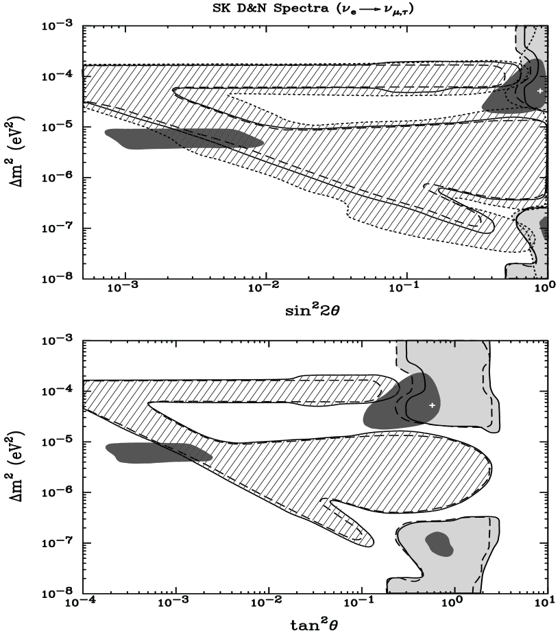
FIG. 1.: The exclusion (hatched) and allowed (lightly shaded) regions at 95% C. L. obtained from the 1258 day SK D&N energy spectra using three different $\chi^{2}$ definitions. The regions enclosed by the dotted (taken from Ref. [12]), dashed and solid lines result from the use of Eqs. (16),(17) and (18), respectively. Equation (18) has no contribution from systematic errors. The flux constraint is imposed to find the allowed regions. The crosshairs mark the best-fit parameters, $(\Delta m^{2},{\rm{tan}^{2}}\theta)=(5.01\times 10^{-5}\,{\rm{eV}^{2}},0.60)$ using Eqs. (17) and (18). The dark shaded regions are the global solutions (with 1117 SK days) at 99% C. L. with free ⁸B and $hep$ fluxes found in Ref. [17].

Another suitable definition of $\chi^{2}$, similar to one used by SK in earlier analyses (of 825 effective days of data), is

$${\chi^{2}(\Delta m^{2},{\rm{tan}^{2}}\theta)}=\sum_{i=1}^{38}\bigg{[}{\big{(}\phi_{i}^{meas}/\phi_{i}^{SSM}-\alpha/(1+\beta\,\sigma_{i}^{corr})\,\phi_{i}^{osc}/\phi_{i}^{SSM}\big{)}^{2}\over(\sigma_{i}^{stat})^{2}+(\sigma_{i}^{uncorr})^{2}}\bigg{]}+\beta^{2}\,,$$ (17)

Again, $\alpha$ is a free flux normalization factor and $\beta$ constrains the variation of correlated systematic errors. Performing a $\chi^{2}$ analysis of the 1258 day data with this definition gives the 95% C. L. exclusion (hatched) region ($\chi^{2}>52.19$ for 37 d.o.f.), outlined by the dashed line in Fig. 1. The $hep$ contribution to the neutrino flux is left unconstrained in the SK analysis while we have fixed the ratio between the $hep$ and ⁸B fluxes. Thus, for a test of the MSW hypothesis, the SK analysis has 36 degrees of freedom while our analysis has 37. Also, keeping in mind that the regions enclosed by the dotted and dashed lines correspond to two different reference solar models and $\chi^{2}$ definitions, it is noteworthy that the general shapes of the regions closely resemble each other, although they differ in size as a consequence of the term $\sum\,(\beta/\sigma_{i}^{corr})^{2}$ in $\chi^{2}_{SK}$. Even if $\beta$ is very small, $\beta\sim 0.001$, the contribution from this term can significantly increase the value of $\chi^{2}_{SK}$ thereby permitting a larger exclusion region. On the other hand, by including the correlated errors in as in (17), their effect is greatly diminished. It is evident that the spectral distortion functions $f_{i}(\beta)$ play an important role in defining an efficient $\chi^{2}$ function. To include the possibility of negative $\Delta m^{2}$, we have also plotted the same region (dashed line) with ${\rm{tan}^{2}}\theta$ as the abscissa [42].

In the approximation that systematic errors can be neglected, both the above $\chi^{2}$ definitions lead to

$${\chi^{2}_{stat}(\Delta m^{2},{\rm{tan}^{2}}\theta)}=\sum_{i=1}^{38}\bigg{[}{\phi_{i}^{meas}/\phi_{i}^{SSM}-\alpha\,\phi_{i}^{osc}/\phi_{i}^{SSM}\over\sigma_{i}^{stat}}\bigg{]}^{2}\,.$$ (18)

The resulting 95% C. L. exclusion region (hatched and enclosed by the solid line) is shown in Fig. 1. Again, we note the remarkable similarity of the shapes of the exclusion regions from the three analyses. Dropping systematic errors leads to a region more similar in size to that obtained by the SK collaboration than that obtained by using Eq. (17). On this basis, we hereafter assume that we can safely ignore all systematic errors when making projections for SNO with simulated data. If SK is a reasonable guide, we will err on the conservative side. It may be counterintuitive that the exclusion region using $\chi^{2}_{SK}$ is larger than that using $\chi^{2}_{stat}$ because one expects more errors to lead to less confidence and therefore a smaller exclusion region. However, as explained earlier, the correlated errors in Eq. 16 are responsible for this. The region using Eq. (17) is smaller than that of $\chi^{2}_{stat}$, in agreement with expectations.

So far we have only considered flux-independent exclusion plots. If instead, flux-dependent allowed regions are sought, one needs to add another term to the $\chi^{2}$ definitions considered,

$${\chi^{2}(\Delta m^{2},{\rm{tan}^{2}}\theta)}\longrightarrow{\chi^{2}(\Delta m^{2},{\rm{tan}^{2}}\theta)}+\bigg{(}{1-\alpha\over\sigma_{\alpha}}\bigg{)}^{2}\,,$$ (19)

where $\sigma_{\alpha}=^{+0.20}_{-0.16}$SSM (or $\rm{SSM}^{\prime}$) is the theoretical uncertainty in the ⁸B flux. In our analysis we symmetrize this value to $\sigma_{\alpha}=\pm 0.18\,$SSM. The 95% C. L. allowed regions ($\Delta\chi^{2}<5.99$ for two oscillation parameters), are superimposed on the exclusion plots in Fig. 1. The allowed region from SK’s analysis is not shown in Ref. [12]; we have taken it from Ref. [43]. It is evident that the allowed regions are alike with minor differences in size. With the $\chi^{2}$-definitions of Eqs. (17) and (18), we find the same best-fit parameters, $(\Delta m^{2},{\rm{tan}^{2}}\theta)=(5.01\times 10^{-5}\,{\rm{eV}^{2}},0.60)$ with $\chi^{2}=30.6$ using Eq. (17) and $\chi^{2}=32.4$ using Eq. (18) for 36 degrees of freedom.

In Fig. 1, the crosshairs represent the best-fit parameters which are very close to those presented by SK from an analysis of the data from 1117 days in which they include the flux constraint [44]; SK does not report the best-fit point from a flux-dependent analysis of the 1258-day D&N spectra. From a flux-independent analysis they find that the minimum $\chi^{2}$ value lies in the VAC region [12], which we have not considered in our analysis. However, from a flux-dependent analysis of their zenith spectrum, they find the minimum $\chi^{2}$ in the VAC region, with some points in the LMA region with similar $\chi^{2}$ values [12]. For example, $(\Delta m^{2},{\rm{tan}^{2}}\theta)=(7\times 10^{-5}\,{\rm{eV}^{2}},0.47)$ is one such point, which is close to our best-fit parameters. A cautionary note when interpreting Fig. 1 is that the dark-shaded flux-independent globally allowed regions of Ref. [17] are not directly comparable to our flux-dependent allowed regions. Our motivation for superimposing the flux-independent allowed regions is to facilitate a comparison with the flux-independent exclusion regions.

IV Data Simulation and Analysis

If the SSM flux is correct, then in the absence of oscillations SNO should detect about 9250 events per year. If instead the SSM flux is wrong and no oscillations occur, the flux suppression expected at SNO is the same as that seen by SK, Eq. (15). We first simulate data assuming this pessimistic scenario and predict the exclusion and allowed regions that we can expect SNO to present three years from now. Then we turn to the more reasonable explanation in which neutrino oscillations do occur.

We simulate data for the best-fit oscillation parameters in each of the three allowed MSW solutions (from the global analysis of Ref. [17]) and display the corresponding exclusion and allowed regions. Exclusion regions are meaningful only when the data points are normally distributed and that for at least some region of the parameter space of interest, $\chi^{2}$/d.o.f $\sim 1$. We enforce this by simulating data for which this is true at the input oscillation parameters. The normalization constant ${{\mathcal{N}}}$ in Eq. (4) is set by the stipulation that we are considering three years of data accumulation.

Figure 2 shows the expected spectra (as a ratio with respect to the SSM) for typical LMA (solid histogram), SMA (dashed histogram) and LOW (dotted histogram) solutions. The data points here are simulated for the LMA solution. For direct comparison of the spectral shapes, these spectra are normalized to the flux corresponding to the simulated data.

FIG. 2.: The expected $e^{-}$ D&N energy spectra at SNO (as a ratio with respect to the SSM) with three years of accumulated data for typical LMA (solid histogram), SMA (dashed histogram) and LOW (dotted histogram) solutions. The data points are simulated for the LMA solution. The spectra are normalized to the flux reflected by the data. The last bin includes all energies from 14 MeV to 20 MeV.

For the sake of specificity, we define $\chi^{2}$ as

$${\chi^{2}(\Delta m^{2},{\rm{tan}^{2}}\theta)}=\sum_{i=1}^{38}\bigg{[}{R^{simulated}_{i}/R^{SSM}_{i}-\alpha\,R_{i}^{osc}/R^{SSM}_{i}\over\sigma_{i}^{stat}}\bigg{]}^{2}\,,$$ (20)

where $\sigma_{i}^{stat}=\sqrt{R^{simulated}_{i}}/R^{SSM}_{i}$ and the number of simulated events, $R^{simulated}_{i}$, in bin $\Delta T_{i}$ is obtained by randomly choosing a point from a Gaussian distribution centered at the theoretical value and of width equal to the square root of the theoretical value. This definition is the same as that of Eq. (19) except that it is expressed in terms of the number of events rather than the flux.

To be conservative, we only show 99% C. L. exclusion ($\chi^{2}>59.89$ for 37 d.o.f.), and allowed regions ($\Delta\chi^{2}<9.21$), resulting from the simulated SNO data. Figure 3 shows the expected regions for the flat spectrum hypothesis (with the same flux suppression as seen by SK) and three MSW solutions. The stars and crosshairs mark the theoretical inputs and best-fit points, respectively. The SMA expectation is characteristic and easily identifiable. For all other possibilities, the plots bear a striking semblance to each other and to the SK results. The LMA and LOW solutions persist simultaneously for all but the SMA solution. The SMA region is excluded to a large extent and with a more efficient $\chi^{2}$ definition, the entire SMA region could be excluded.

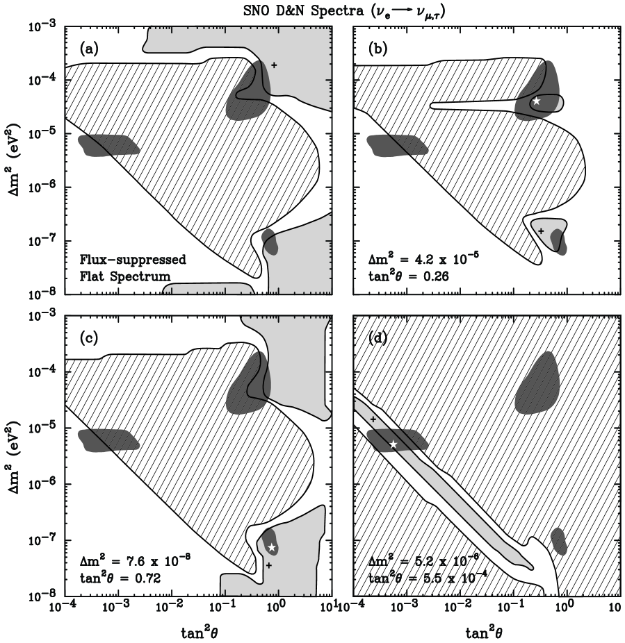
FIG. 3.: Expected 99% C. L. exclusion (hatched) and allowed (lightly shaded) regions from the D&N spectra at SNO for (a) a flux-suppressed flat spectrum (b) LMA solution, (c) LOW solution and (d) SMA solution with three years of accumulated data. The dark shaded regions are the global solutions at 99% C. L. with free ⁸B and $hep$ fluxes. The stars and crosshairs mark the theoretical inputs and best-fit points, respectively.

V Zenith Angle Distribution

In principle the information contained in the zenith angle distribution is contained in the D&N spectra. The SK exclusion regions obtained by them in separate analyses of the D&N spectra and the zenith angle distribution (with energy subdivisions) bear testimony to this expectation; the differences are small [12]. This is despite the fact that each zenith angle bin is split into several energy bins, thereby potentially maximizing the resolution available to SK. It has been advocated that an appropriate choice of binning might make it possible for SNO to not only identify which solution is correct but also to determine the oscillation parameters [24]. By performing a complete analysis, we now assess the extent to which this claim can be validated.

The choice of night bins of equal size in cos$\,\theta_{Z}$ is democratic, but does not take advantage of any distinctive features of the distributions of the different solutions. In the context of SNO, the qualitative behavior of the distributions for the LMA, SMA and LOW solutions was studied in detail in Ref. [24]. It was found that with a suitable choice of binning, any smearing of peculiarities intrinsic to the region of parameter space can be avoided. The events were binned in a manner that leads to a characteristic distribution for the LOW solution because in the SMA and LMA regions, the cos$\,\theta_{Z}$-dependence is rather weak leading to a more or less flat distribution. This remark is pertinent, since as we have seen, it is difficult to differentiate the LMA and LOW solutions from each other. If the SMA solution is the correct one, the strong spectral distortion will easily make it stand apart. As defined in Table I, there is one day bin and five non-uniform night bins. The “core bin”, N5, at SNO ((cos$\,\theta_{Z})_{max}=0.92$) is smaller than that at SK ((cos$\,\theta_{Z})_{max}=0.975$) because SNO’s higher latitude restricts the $\theta_{Z}$ range. Thus, a smaller number of solar neutrinos that pass through the Earth’s core are incident at SNO than at SK.

$$\begin{array}[]{lrcccl}\rm{Dataset}&&&&&\\ \hline\cr\rm{Day}&-1&\leq&{\rm{cos}}\,\theta_{Z}&\leq&0\\ \rm{N1}&0&<&{\rm{cos}}\,\theta_{Z}&\leq&0.173\\ \rm{N2}&0.173&<&{\rm{cos}}\,\theta_{Z}&\leq&0.5\\ \rm{N3}&0.5&<&{\rm{cos}}\,\theta_{Z}&\leq&0.707\\ \rm{N4}&0.707&<&{\rm{cos}}\,\theta_{Z}&\leq&0.83\\ \rm{N5}&0.83&<&{\rm{cos}}\,\theta_{Z}&\leq&0.92\end{array}$$ (28)

TABLE I.: The definitions of the night bins in terms of the nadir of the Sun, $\theta_{Z}$. Note that the “core bin”, N5, does not contain zeniths beyond 0.92 because the latitude of the detector restricts its range.

Since we know the zenith-angle exposure function [28], the SSM prediction for the number of events in each zenith angle bin, $R_{i,SSM}^{Z}$, and the prediction with oscillations, $R_{i,\,osc}^{Z}$, can be calculated. For a given set of oscillation parameters, we want to generate zenith angle distributions that have the same number of events as the simulated energy spectra of the previous section. The number of events in the day bin is simply the sum of all the events in the day spectrum. For the night bins, we use $R_{i,\,osc}^{Z}$ as the central value of a Gaussian distribution and simulate the number of events in each night bin. Note that the number of events at night represented by this distribution does not coincide with that of the night spectrum. The nighttime distribution is renormalized to yield the number of events in the night spectrum. Now the simulated energy spectra and zenith angle distribution reflect the same data. To match the number of simulated events in the zenith angle distribution and the D&N spectra, two normalizations are needed, one each for the daytime and nighttime events. The shape of the theoretical expectation, however involves only one normalization, namely, the total number of simulated events.

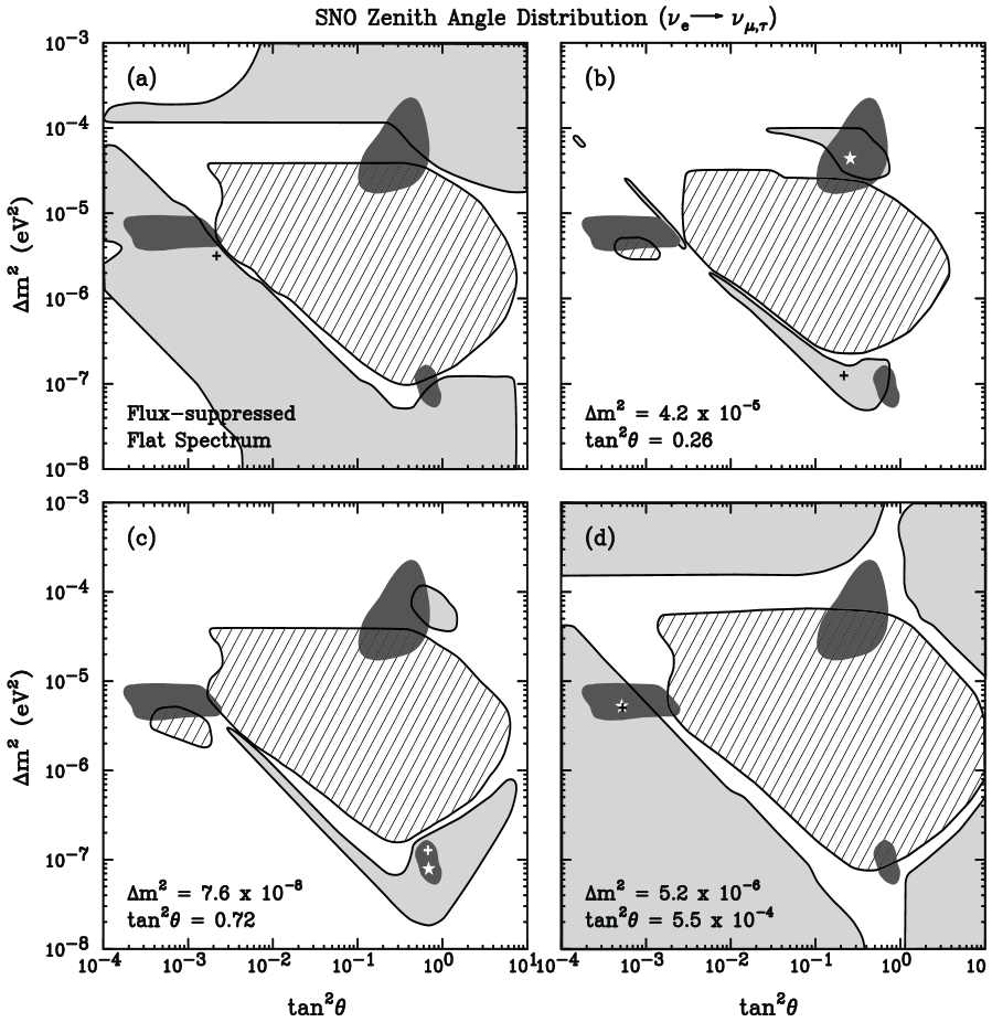
FIG. 4.: Expected 99% C. L. exclusion (hatched) and allowed (lightly shaded) regions from zenith angle distributions at SNO corresponding to the simulated datasets of Fig. 3. The stars and crosshairs mark the theoretical inputs and best-fit points, respectively.

We perform flux-independent analyses (for the same datasets used to find the regions of Fig. 3) with the simple $\chi^{2}$ function,

$${\chi^{2}(\Delta m^{2},{\rm{tan}^{2}}\theta)}^{Z}=\sum_{i=1}^{6}\,\bigg{[}{R_{i,\,simulated}^{Z}/R_{i,\,SSM}^{Z}-\alpha\,R_{i,\,osc}^{Z}/R_{i,\,SSM}^{Z}\over\sigma_{i}^{Z}}\bigg{]}^{2}\,,$$ (29)

where $\sigma_{i}^{Z}=\sqrt{{R_{i,simulated}^{Z}}}/R_{i,SSM}^{Z}$. From Fig 4, it is evident that the zenith angle distributions of the various solutions lead to similar 99% C. L. exclusion regions ($\chi^{2}>15.09$ for 5 d.o.f.). We underscore the fact that the regions corresponding to the flat spectrum, LMA and LOW datasets exclude part of the SMA region, and that the region found with the SMA dataset excludes a large part of the LMA and LOW solutions. This is consistent with Fig. 3. Additionally, the 99% C. L allowed regions have the same shapes for the LMA and LOW solutions. The flux constraint is included to find the allowed regions. The stars and crosshairs mark the theoretical inputs and best-fit points, respectively.

Figure 5 shows the 99% C. L. exclusion ($\chi^{2}>16.81$ for 6 d.o.f.), and allowed regions from the zenith angle distribution from 1258 days of data at SK. In making these regions, we have employed SK’s binning which is different from our choice for SNO. The statistical and systematic errors are added in quadrature. The crosshairs mark the best-fit parameters, $(\Delta m^{2},{\rm{tan}^{2}}\theta)=(5.01\times 10^{-5}\,{\rm{eV}^{2}},0.56)$ with $\chi^{2}=5.15$. The exclusion regions of Figs. 4–5 are similar to the 99% C. L. exclusion region reported by SK (with a 504-day dataset) with a similar $\chi^{2}$ definition [45]. No parts of the globally allowed regions are excluded. Of course, subdividing each zenith angle bin into energy bins (as done by SK in their latest analysis [12]) will greatly improve the sensitivity of the analysis, but this is equivalent to using D&N energy spectra.

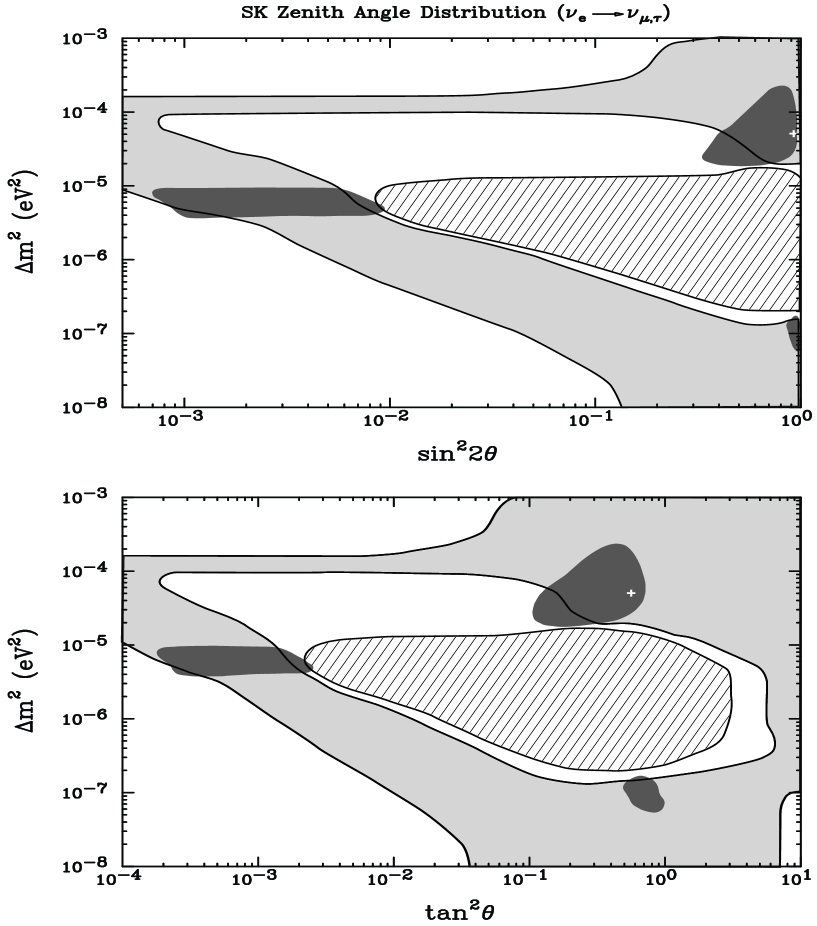
FIG. 5.: The exclusion (hatched) and allowed (lightly shaded) regions at 99% C. L. from the 1258-day SK zenith angle distribution. The crosshairs mark the best-fit parameters, $(\Delta m^{2},{\rm{tan}^{2}}\theta)=(5.01\times 10^{-5}\,{\rm{eV}^{2}},0.56)$.

The day-night variation embodied in the zenith angle distribution can also be presented in terms of a day-night asymmetry defined by

$$A_{DN}=2\,{N-D\over N+D}=2\,{P^{N}-P^{D}\over P^{N}+P^{D}}\,,$$ (30)

where $D$ and $N$ are the total number of events detected during the days and nights, respectively. The approximate ranges of $A_{DN}$ are $(0.005,0.1)$ in the LMA and LOW regions and $(-0.01,0.05)$ in the SMA region. Note that in parts of the SMA region, $A_{DN}<0$, thus uniquely identifying the SMA solution. However, $A_{DN}>-0.01$ and an identification of such a small deviation from zero will be difficult. Semi-analytic approximations for $A_{DN}$ have been derived for the three allowed regions [25]. These expressions can be used to provide insight into the orientations of the zenith-angle allowed regions. Iso-asymmetry lines in $A_{DN}$ that pass through all three regions must have $A_{DN}>0$ and are given by

$$\Delta m^{2}\,({\rm{eV}^{2}}) \approx {3\times 10^{-6}}\,{{\rm{sin}}^{2}2\,\theta\over A_{DN}}\ \ \ \ \ \ \ \ (\rm{LMA})\,,$$ (31)

$$A_{DN} \approx {\rm{sin}}^{2}2\,\theta\ \ \ \ \ \ \ \ \ \ \ \ \ \ \,\ \ \ \ \ \ (\rm{SMA})\,,$$ (32)

$$\Delta m^{2}\,({\rm{eV}^{2}}) \approx 2.5\times 10^{-6}\,{A_{DN}\over{\rm{sin}}^{2}2\,\theta}\ \ \ \ \ \ (\rm{LOW})\,.$$ (33)

The relations in Eqs. (31–33) have a wider domain of applicability than indicated. For example, Eq. (33) is applicable in the range $10^{-8}\mathrel{\raise 1.29167pt\hbox{$<$\kern-7.5pt\lower 4.30554pt\hbox{$\sim$}}}\Delta m^{2}\mathrel{\raise 1.29167pt\hbox{$<$\kern-7.5pt\lower 4.30554pt\hbox{$\sim$}}}3\times 10^{-6}$. This explains why the 99% C. L. allowed regions almost connect the SMA and LOW solutions.

VI Summary

We have analyzed the 1258-day day and night energy spectra presented by Super-Kamiokande using $\chi^{2}$ definitions that account for systematic errors in different ways. The best-fit lies in the LMA region at $(\Delta m^{2},{\rm{tan}^{2}}\theta)=(5.01\times 10^{-5}\,{\rm{eV}^{2}},0.60)$, independently of whether systematic errors are included in the $\chi^{2}$-definition. We have shown that these approaches lead to exclusion and allowed regions of different sizes, but the general areas of the regions remain unchanged even if systematic errors are neglected (see Fig. 1). Using Super-Kamiokande as our reference, we then draw conclusions for SNO based on analyses that incorporates only statistical errors. We assume the optimistic electron kinetic energy threshold of 5 MeV and three years of accumulated data.

If the SMA solution is correct, the day and night spectra will show sufficiently strong distortions to distinguish it from the other solutions (Fig. 3(d)). For a flux-suppressed flat spectrum or the LMA and LOW solutions, the regions are similar enough to not provide any constraint beyond the exclusion of most of the the SMA solution (Fig. 3(a–c)); the LMA and LOW solutions are indistinguishable. However, KamLAND [19] will certainly help in this regard by either ruling out the LMA solution or pinning down the LMA oscillation parameters [20]. The zenith angle distribution in itself will not add anything to what can be obtained from the day and night spectra unless each zenith angle bin is subdivided into energy bins.

The 99% C. L. exclusion regions in Fig. 4 bear a striking similarity to that obtained from the 1258-day zenith angle distribution at Super-Kamiokande (Fig. 5), for which the best-fit parameters are $(\Delta m^{2},{\rm{tan}^{2}}\theta)=(5.01\times 10^{-5}\,{\rm{eV}^{2}},0.56)$. We expect results from charged-current measurements at SNO to be similar to that of Super-Kamiokande, thus providing an important check of the Super-Kamiokande conclusions. Needless to say, neutral current data from SNO will provide a crucial test of the existence of sterile neutrinos, and if solar neutrinos do not oscillate to sterile neutrinos, SNO will measure the ⁸B flux produced in the Sun.

- [1] K. Hirata et al., Phys. Lett. B205, 416 (1988); Phys. Lett. B280, 146 (1992).
- [2] Y. Fukuda et al., Phys. Lett. B433, 9 (1998); Phys. Rev. Lett. 81, 1562 (1998); Phys. Rev. Lett. 82, 2644 (1999); Phys. Lett. B467, 185 (1999).
- [3] D. Casper et al., Phys. Rev. Lett. 66, 2561 (1991); R. Becker-Szendy et al., Phys. Rev. D46, 3720 (1992); Phys. Rev. Lett. 69, 1010 (1992).
- [4] W. Allison et al., Phys. Lett. B391, 491 (1997); Phys. Lett. B449, 137 (1999).
- [5] M. Ambrosio et al., Phys. Lett. B434, 451 (1998); hep-ex/0001044.
- [6] J. Bahcall, Neutrino Astrophysics (Cambridge University Press, Cambridge, England, 1989).
- [7] B. Cleveland, T. Daily, R. Davis, Jr., J. Distel, K. Lande, C. Lee, P. Wildenhain and J. Ullman, Astropart. Phys. 496, 505 (1998).
- [8] J. Abdurashitov et al., Phys. Rev. C60, 055801 (1999).
- [9] W. Hampel et al., Phys. Lett. B447, 127 (1999).
- [10] M. Altmann et al., Phys. Lett. B490, 16 (2000).
- [11] S. Fukuda et al., hep-ex/0103032.
- [12] S. Fukuda et al., hep-ex/0103033.
- [13] J. Bahcall, M. Pinsonneault and S. Basu, astro-ph/0010346.
- [14] L. Wolfenstein, Phys. Rev. D17, 2369 (1978); V. Barger, K. Whisnant, S. Pakvasa and R. Phillips, Phys. Rev. D22, 2718 (1980).
- [15] S. Mikheyev and A. Yu. Smirnov, in Massive Neutrino in Astrophysics and in Particle Physics, Proceedings of the Moriond Workshop, Tignes, Savoie, France, 1986, edited by O. Fackler and J. Tran Thanh Van (Editions Frontières, Gif-sur-Yvette, France, 1986), p. 355.
- [16] A. Baltz and J. Weneser, Phys. Rev. D35, 528 (1994); Phys. Rev. D37, 3364 (1988).
- [17] J. Bahcall, P. Krastev and A. Yu. Smirnov, hep-ph/0103179.
- [18] G. Fogli, E. Lisi, D. Montanino and A. Palazzo, Phys. Rev. D62, 013002 (2000); M. Gonzalez-Garcia, M. Maltoni, C. Pena-Garay and J. Valle, Phys. Rev. D63, 033005 (2001); J. Bahcall, P. Krastev and A. Yu. Smirnov, Phys. Rev. D60, 093001 (1999); J. Bahcall, P. Krastev and A. Yu. Smirnov, Phys. Rev. D58, 096016 (1998); N. Hata and P. Langacker, Phys. Rev. D56, 6107 (1997).
- [19] KamLAND proposal, Stanford-HEP-98-03.
- [20] V. Barger, D. Marfatia and B. Wood, Phys. Lett. B498, 53 (2001).
- [21] R. Barbieri and A. Strumia, hep-ph/0011307; H. Murayama and A. Pierce, hep-ph/0012075.
- [22] A. McDonald, Nucl. Phys. B (Proc. Suppl) 77, 43 (1999); J. Boger et al. Nucl. Instrum. Meth. A449, 172 (2000).
- [23] J. Bahcall, P. Krastev and A. Yu. Smirnov, Phys. Rev. D62, 093004 (2000); M. Maris and S. Petcov, Phys. Rev. D62, 093006 (2000); J. Bahcall, P. Krastev and A. Yu. Smirnov, Phys. Lett. B477, 401 (2000); M. Gonzalez-Garcia and C. Pena-Garay, hep-ph/0011245; G. Fogli, E. Lisi and D. Montanino, Phys. Lett. B434, 333 (1998); W. Kwong and S. Rosen, Phys. Rev. D54, 2043 (1996).
- [24] M. Gonzalez-Garcia, C. Pena-Garay and A. Yu. Smirnov, hep-ph/0012313.
- [25] J. Bahcall, P. Krastev and A. Yu. Smirnov, Phys. Rev. D63, 053012 (2000).
- [26] M. Apollonio et al., Phys. Lett. B466, 415 (1999); Phys. Lett. B420, 397 (1998).
- [27] F. Boehm et al., Phys. Rev. D62, 072002 (2000); Phys. Rev. Lett. 84, 3764 (2000).
- [28] J. Bahcall and P. Krastev, Phys. Rev. C56, 2839 (1997).
- [29] C. Ortiz, A. Garcia, R. Waltz, M. Bhattacharya and A. Komives, Phys. Rev. Lett. 85, 2909 (2000). http//www.nd.edu/~nsl/BeyondSM/boron8/
- [30] J. Bahcall, S. Basu and M. Pinsonneault, Phys. Lett. B433, 1 (1998).
- [31] L. Marcucci, R. Schiavilla, M. Viviani, A. Kievsky and S. Rosati, Phys. Rev. Lett. 84, 5959 (2000).
- [32] S. Parke, Phys. Rev. Lett. 57, 1275 (1986).
- [33] S. Petcov, Phys. Lett. B200, 373 (1998); Phys. Lett. B214, 139 (1998).
- [34] W. Haxton, Phys. Rev. Lett. 57, 1271 (1986); Phys. Rev. D35, 2352 (1987).
- [35] A. Dziewonski and D. Anderson, Phys. Earth Planet. Inter. 25, 297 (1981).
- [36] J. Bahcall and E. Lisi, Phys. Rev. D54, 5417 (1996).
- [37] F. Villante, G. Fiorentini and E. Lisi, Phys. Rev. D59, 013006 (1999).
- [38] G. Fogli, E. Lisi, A. Palazzo and F. Villante, hep-ph/0102288.
- [39] J. Bahcall, M. Pinsonneault and S. Basu, astro-ph/0010346 v1.
- [40] J. Bahcall, M. Kamionkowsky and A. Sirlin, Phys. Rev. D51, 6146 (1995).
- [41] J. Bahcall, E. Lisi, D. Alburger, L. De Braeckeleer, S. Freedman and J. Napolitano, Phys. Rev. C54, 411 (1996).
- [42] G. Fogli, E. Lisi and D. Montanino, Phys. Rev. D54, 2048 (1996); A. Gouvea, A. Friedland and H. Murayama, Phys. Lett. B490, 125 (2000).
- [43] M. Smy, talk at NOON 2000, The Workshop on Neutrno Oscillations and Their Origin, Tokyo, Japan, December 2000.
- [44] Y. Suzuki, talk at Neutrino 2000, XIXth International Conference on Neutrino Physics and Astrophysics, Sudbury, Canada, June 2000.
- [45] Y. Fukuda et al., Phys. Rev. Lett. 82, 1810 (1999).