Abstract

Unintegrated gluon densities in nuclei, dipole-nucleus cross-sections and quark densities are numerically investigated in the high-colour limit, with the scattering on a heavy nucleus exactly described by the sum of fan diagrams of BFKL pomerons. The initial condition for the evolution in rapidity is quickly forgotten, and the gluon density presents a ”supersaturation” pattern, as previous studies indicated. Both dipole-nucleus cross-sections and quark densities present the expected saturation features. Identifying the position in transverse momentum $l$ of the maximum of the gluon distribution with the saturation momentum $Q_{s}(y,b)$, at large rapidities all distributions depend only on one variable $[l/Q_{s}(y,b)]$ or $[rQ_{s}(y,b)]$.

1 Introduction

In view of the current and forthcoming experimental investigations of the strong interaction with heavy nuclei at high energies, much attention has lately been devoted to the theoretical study of parton distributions inside a heavy nucleus at small values of the scaling variable $x$. It turned out that a particularly transparent approach follows from the colour dipole picture [1,2], in which the interaction of a probe with a target is presented via the interaction of the latter with a colour dipole, convoluted with the distribution of colour dipoles in the probe. In such a picture the fundamental quantity is the cross-section $\sigma(Y,r)$ for the interaction of a colour dipole of a given transverse radius $r$ with a target at a given rapidity $Y$. Much popularity has obtained the idea of ”saturation”, which in terms of the cross-section $\sigma$ implies that at high energies the cross-section $\sigma(Y,r)$ tends to a constant independent of $r$ [3]. A particular ansatz chosen in [3] for the scattering of a dipole on the proton,

$$\sigma_{p}(Y,r)=\sigma_{0}\left(1-e^{-\hat{r}^{2}}\right),\ \ \hat{r}=\frac{r}{2R_{0}(Y)}\ ,$$ (1)

with $\sigma_{0}\simeq 23$ mb and $R_{0}$ diminishing with increasing rapidity $Y$, leads to a good description of the DIS data for the proton below $x=0.01$.

A less phenomenological treatment can be applied for the heavy nucleus target. In the framework of the colour dipole model it follows that, in the high-colour limit $N_{c}\to\infty$, the scattering on a heavy nucleus is exactly described by the sum of fan diagrams constructed of BFKL pomerons, each of them splitting into two. The resulting equation for the colour dipole cross-section on the nucleus [4-7] was numerically solved in [7]. The gluon density introduced in [7] revealed a ”supersaturation” behaviour, tending to zero at any fixed momentum $k$ as $Y\to\infty$. As a function of $\ln k$ it proved to have a form of a soliton wave moving to the right with a constant velocity as $Y$ increases. A more ambitious project is currently developed by the McLerran group, which can, in principle, lead to a description which does not employ the large number of colors limit [8-10]. Admitting that such an improvement is highly desirable, we think that the $N_{c}\to\infty$ approach is much more feasible and can give a clear hint on the qualitative behaviour of parton densities and cross-sections for the heavy nucleus target.

In this paper we continue studying the numerical solution of the BFKL fan diagram equation started in [7], with more precision and more attention to rapidities available at present or in the near future. We compare solutions obtained from a purely theoretical initial function (as in [7]) and from a phenomenologically supported one (like Eq. (1)). We find that the initial form is very quickly forgotten by the equation, so that at rapidities of the order 10 the solution becomes independent of the chosen initial form. The behaviour of the solution at large energies is completely determined by the scale $Q_{s}(Y,b)$, depending on the energy and impact parameter $b$, at which the gluon density reaches its maximum value, so that both the parton densities and the dipole cross-section become universal functions of momentum or coordinate scaled with $Q_{s}$. One may consider $Q_{s}$ as a ”saturation momentum” introduced in [4,8,11]. The $Y$ and $b$ dependence of $Q$ which follow from our numerical studies can be fitted by a simple formula:

$$\ln Q_{s}=a+cy+d\ln[AT(b)],\ \ \ y=\frac{N_{c}\alpha_{s}}{\pi}Y,$$ (2)

with

$$c=2.06,\ \ d=0.62\pm 0.07,$$

$Q_{s}$ in GeV/c, and $T(b)$ the nuclear profile function in (GeV/c)^-2 defined so that $\int d^{2}b\,T(b)=1$; thus, $AT(b)\propto A^{1/3}$. Note that the value of $c$ results lower than in our previous run devoted mostly to asymptotic energies and agrees with the predictions in [12] based on asymptotic estimates. The somewhat unexpected value of $d$ seems to slightly depend on the choice of the initial function (hence the $\pm 0.07$). It implies that $Q_{s}\propto A^{\alpha}$, $\alpha\simeq 2/9$. The dipole cross-section on the nucleus at fixed impact parameter exhibits the expected behaviour, tending to unity at each $r$ as $Y\to\infty$. The quark density follows the pattern of saturation, tending to a constant value at small momenta, in full agreement with the predictions of [13].

2 The evolution equation and initial conditions

As mentioned, in the colour dipole approach the cross-section of a probe ($P)$ on the nucleus ($A$) is presented via the dipole cross-section:

$$\sigma_{PA}(Y)=\int d^{2}r\rho_{P}(r)\sigma_{A}(Y,r).$$ (3)

In its turn, the dipole cross-section on the nucleus is an integral over the impact parameter:

$$\sigma_{A}(Y,r)=2\int d^{2}b\Phi(Y,r,b),$$ (4)

where evidently $2\Phi$ has a meaning of a cross-section at fixed impact parameter. The evolution equation in $Y$ can be most conveniently written for the function

$$\phi(Y,r,b)=\frac{1}{2\pi r^{2}}\Phi(Y,r,b)$$ (5)

in momentum space, where it reads [7]

$$\left(\frac{\partial}{\partial y}+H_{BFKL}\right)\phi(y,q,b)=-\phi^{2}(y,q,b),$$ (6)

with a rescaled rapidity $y$ given in Eq. (2) and $H_{BFKL}$ the BFKL Hamiltonian.

Special attention has to be devoted to the initial function $\phi(y_{0},q,b)=\phi_{0}$ at $y=y_{0}$, from which value one is starting the evolution. In the framework of the pure BFKL approach, with $N_{c}\to\infty$ and $A$ fixed, one should choose $y_{0}=0$ (or any finite $y$) and take for $\phi_{0}$ the contribution of the pure two gluon exchange with a single nucleon inside the nucleus. If $A$ is large ($A^{1/3}$ of the same order as $N_{c}$) then one should add all multiple interactions inside the nucleus, which sum into a Glauber cross-section:

$$\Phi_{0}(r,b)=1-e^{-AT(b)\sigma_{p}(0,r)}.$$ (7)

Here $\sigma_{p}(0,r)$ is the dipole-proton cross-section generated by the two-gluon exchange:

$$\sigma_{p}(0,r)=\frac{1}{2}g^{4}\int d^{2}r^{\prime}G(0,r,r^{\prime})\rho_{p}(r^{\prime}),$$ (8)

where $\rho_{p}(r)$ is the colour dipole density in the proton and $G(0,r,r^{\prime})$ is the BFKL Green function at $Y=0$:

$$G(0,r,r^{\prime})=\frac{rr^{\prime}}{8\pi}\frac{r_{<}}{r_{>}}\left(1+\ln\frac{r_{>}}{r_{<}}\right),\ \ r_{>(<)}={\rm max(min)}\{r,r^{\prime}\}.$$ (9)

Obviously the density $\rho_{p}$ is non-perturbative and not known. As in [7], to simplify the calculations we choose $\rho_{p}$ to be a normalized Yukawa distribution

$$\rho_{p}(r)=\frac{\mu}{2\pi}\frac{e^{-\mu r}}{r}\ ,$$ (10)

with $\mu=0.3$ GeV adjusted to the nucleon radius value. With Eq. (10) we find

$$AT(b)\sigma_{p}(0,r)=B\left[2{\rm C}-1+2\ln\tilde{r}-{\rm Ei}(-\tilde{r})\left(2+\tilde{r}^{2}\right)+e^{-\tilde{r}}(1-\tilde{r})\right],\ \ \tilde{r}=\mu r,$$ (11)

where C is the Euler constant and dimensionless $B$ carries all the information about the nucleus. For Pb at the center ($b=0$) it reaches the value 0.12. Of course, this choice of $\rho_{p}$ may look rather arbitrary. We noted in [7] that calculations demonstrated a certain indifference of the evolution equation to the choice of the initial function at high enough $y$. To see this more clearly, in this run we also used an alternative initial function, more adjusted to the existing experimental data at comparatively small rapidities. A natural choice would be to take directly (1). However its analytic form makes it rather difficult to pass to the momentum space employed in our method of evolution. Therefore we choose a slightly different form for the phenomenologically motivated initial dipole cross-section on the nucleon:

$$AT(b)\sigma^{ph}_{p}=B\left(1-e^{-\hat{r}}\right)^{2},$$ (12)

with the same parameters as in [3] and $Y_{0}$ corresponding to $x=0.01$. The cross-section in Eq. (12) has the same asymptotic behaviour as that in Eq. (1), both at $r\to 0$ and $r\to\infty$. For finite $r$ it is slightly different, but this difference is not too large and, after all, the choice (1) is also quite ad hoc. Note that the asymptotic behaviour of the phenomenological cross-section is different from that of Eq. (11), which both at $r\to 0$ and $r\to\infty$ contains an extra $|\ln r|$ factor. The dimensionless $B$ in Eq. (12) results substantially larger than for Eq. (11) and is of the order of 5 for Pb at the center.

However, as we shall presently see, in spite of the difference both in the asymptotic behaviour and in the overall normalization, starting from $y\sim 2$ the results of the evolution begin to look practically identical for both choices of the initial function, except for the overall scale $Q_{s}$ mentioned in the Introduction.

3 The gluon density and dipole cross-sections

We define the gluon density as in [7]:

$$\frac{\partial[xG(x,k^{2},b)]}{\partial^{2}b\partial k^{2}}=\frac{2N_{c}}{\pi g^{2}}k^{2}\nabla_{k}^{2}\phi(y,k,b)\equiv\frac{2N_{c}}{\pi g^{2}}h(y,k,b),$$ (13)

with $y=(N_{c}\alpha_{s}/\pi)\ln(1/x)$. This definition follows the logic of the BFKL approach in which it corresponds to the average of two gluon fields in the nucleus, in the axial gauge adopted in this approach. It also naturally appears in the expression for the structure function of the nucleus (see [7]). There exist different definitions of the gluon density in the literature (see [13]). We are not going to discuss the problem of a ”correct” gluon density here, since in any case it is not a directly measurable quantity, but rather serves to calculate the latter (see comments in [14]). From a pragmatic point of view our definition is well supported, since all observables can be directly related to (13).

The results of our evolution for the gluon density are shown in Figures 1 and 2. Not to bind ourselves to a particular value of the coupling constant $\alpha_{s}$, we rather present $h(y,k,b)$ as a function of the rescaled rapidity $y$. The actual gluon density at physical rapidity is obtained after rescaling both $h$ and $y$ according to Eqs. (2) and (13).

In Fig. 1 we show the gluon densities at the first stage of the evolution up to $y=1$, starting from the initial functions corresponding to the Glauberized two-gluon exchange contribution (11) (theoretical initial function, TIF) and to the phenomenological cross-section (12) (phenomenological initial function, PIF), respectively. One observes a large difference between the two at the beginning of the evolution, which, however, is gradually disappearing. Starting from $y\sim 2$ the form of the gluon distribution becomes practically identical for both initial functions. We introduce $Q_{s}(y,b)$ as the the momentum at which the density reaches its maximum. For the two initial functions a numerical fit gives Eq. (2) with $a=-2.21$ $(-0.88)$ , $c=2.09$ $(2.04)$ and $d=0.69$ $(0.55)$ for TIF (PIF). Plotted against $k/Q_{s}(y,b)$ the gluon distributions for both initial functions and for all values of $b$ and $y>2$ practically fall onto a universal curve. The degree of universality is illustrated in Fig. 2 where we present the gluon densities for both TIF and PIF at $y=2.4$ and 4, and at $b=0$ and $b=0.98R_{A}$, for the Pb target. Some differences in the curves are certainly visible, which however diminish as $y$ grows. The form of the universal curve can be fitted by an expression

$$h(\xi)=0.295\exp{\left(-\frac{(\xi-\xi_{0})^{2}}{4\cdot 0.869}\right)},\ \ \xi=\ln{k},\ \ \xi_{0}=\ln{Q_{s}(y,b)}$$ (14)

(all momenta in GeV/c), from which one observes that the density falls as a function of momentum both at $k\to 0$ and $k\to\infty$.

The gluon density (13) is trivially related to the dipole cross-section on the nucleus at fixed $b$:

$$\Phi(y,r,b)=1-\int\frac{d^{2}k}{2\pi k^{2}}h(y,k,r)e^{i{\bf kr}}.$$ (15)

So, to determine $\Phi$, all one has to do is to perform a Bessel transform of $h/k$. Fig. 3 shows the dipole cross-sections at low rapidities. At larger rapidities $y>2$ the scaling properties of $h$ imply that $\Phi$ becomes a universal function of $rQ_{s}(y,b)$. Its form is illustrated in Fig. 4, where we show $\Phi(r)$ for Pb at $b=0$ and $y=3.4$ (for PIF). It can be fitted with a formula

$$\Phi(r)=\left[1-\exp{\left(-\omega^{2}r^{2}\right)^{1/\delta}}\right]^{\delta},\ \ \omega=198.5\ {\rm GeV/c},\ \ \delta=5.48.$$ (16)

4 The quark density

The definition of the quark density can be taken from [13]:

$$\frac{\partial[xq(x,l,b)]}{\partial^{2}l\partial^{2}b}=\frac{\alpha_{s}Q^{2}}{(2\pi)^{3}}\int_{0}^{1}d\alpha d^{2}b_{1}d^{2}b_{2}e^{-i{\bf l(b_{1}-b_{2})}}$$

$$\left[\left(\alpha^{2}+(1-\alpha)^{2}\right)\epsilon^{2}\frac{{\bf b_{1}b_{2}}}{b_{1}b_{2}}{\rm K}_{1}(\epsilon b_{1}){\rm K}_{1}(\epsilon b_{2})+4Q^{2}\alpha^{2}(1-\alpha)^{2}{\rm K}_{0}(\epsilon b_{1}){\rm K}_{0}(\epsilon b_{2})\right]$$

$$\int\frac{d^{2}k}{(2\pi)^{2}}\frac{1}{k^{2}}\frac{\partial[xG(x,k,b)]}{\partial^{2}b\partial k^{2}}\left[1+e^{-i{\bf k(b_{1}-b_{2})}}-e^{-i{\bf kb_{1}}}-e^{i{\bf kb_{2}}}\right],$$ (17)

with $\epsilon^{2}=Q^{2}\alpha(1-\alpha)$. This definition is based on the form of the interaction with the target of a virtual current which splits into a $q\bar{q}$ pair. For the small $x$ region one may also raise objections as to its physical meaning, since then the interference diagram gives a non-zero contribution [14]. However, for lack of a better definition, we shall use Eq. (17).

Performing part of the integrations and using Eq. (13), we express the quark density as

$$\frac{\partial[xq(x,l,b)]}{\partial^{2}l\partial^{2}b}=\pi^{4}f(y,l,b),\ \$$ (18)

where $y=(N_{c}\alpha_{s}/\pi)\ln(1/x)$ and function $f$, independent of the coupling constant, is given by an integral over momenta:

$$f(y,l,b)=\frac{N_{c}}{8\pi^{8}}\int_{0}^{\infty}\frac{dk}{k}h(y,k,b)I(l,k).$$ (19)

Here $I$ is a sum of transversal ($T$) and longitudinal ($L$) parts, with

$$I_{T}=Q^{2}\int_{0}^{1}d\alpha\left[\alpha^{2}+(1-\alpha)^{2}\right]\left[\left(2\epsilon^{2}+k^{2}\right)\chi\lambda-\epsilon^{2}\left(\epsilon^{2}+l^{2}+k^{2}\right)\chi^{3}-\epsilon^{2}\lambda^{2}\right]$$ (20)

and

$$I_{L}=4Q^{4}\int_{0}^{1}d\alpha^{2}\alpha(1-\alpha)^{2}\left[\left(\epsilon^{2}+l^{2}+k^{2}\right)\chi^{3}+\lambda^{2}-2\chi\lambda\right],$$ (21)

where

$$\lambda=\frac{1}{\epsilon^{2}+l^{2}}\ ,\ \ \chi=\frac{1}{\sqrt{\left(\epsilon^{2}+(l+k)^{2}\right)\left(\epsilon^{2}+(l-k)^{2}\right)}}\ .$$ (22)

Note that the quark density defined by Eqs. (17)-(22) depends (weakly) on the virtuality of the probe $Q^{2}$. Physically meaningful results correspond to the limiting case $Q^{2}\to\infty$. In this limit the longitudinal part of $I$ gives no contribution and in the transversal part the integration over $\alpha$ is reduced to that over $\epsilon^{2}$:

$$Q^{2}\int_{0}^{1}d\alpha\left[\alpha^{2}+(1-\alpha)^{2}\right]\to 2\int_{0}^{\infty}d\epsilon^{2},$$ (23)

so that $I$ and $f$ become independent of $Q^{2}$.

These formulas give the quark density in terms of the gluon density, that is, in terms of the function $h$, which we have found numerically. Doing the integration over $k$ in Eq. (19) also numerically, we obtain function $f$ and therefore the quark density related to it by a factor (see Eq. (18)). Our results for the quark density (in fact for $f$) are presented in Figs. 5 and 6. As before, in Fig. 5 we show the quark densities at the beginning of the evolution for the initial functions TIF and PIF respectively. At higher $y>2$ and due to scaling properties of the gluon density, the quark density also becomes a universal function of $l/Q_{s}(y,b)$. Its form is illustrated in Fig. 6, where we show $f(l)$ for Pb at $b=0$ and $y=3.6$ (for PIF). It can be fitted by

$$f(t)=\frac{N_{c}}{2\pi^{8}}\frac{\left[1-\exp{\left(-t^{1/\beta}\right)}\right]^{\beta}}{t}\ ,\ \ t=2\left(\frac{l}{511.0\ {\rm GeV/c}}\right)^{2},\ \ \beta=2.44.$$ (24)

Note that at $l\to 0$ the quark densities tend to a constant value in agreement with the prediction of A. H. Mueller [13]:

$$\frac{\partial[xq(x,l,b)]}{\partial^{2}l\partial^{2}b}\longrightarrow_{l\to 0}\frac{N_{c}}{2\pi^{4}}\ ,$$ (25)

which implies

$$f(l)\longrightarrow_{l\to 0}1.58\cdot 10^{-4};$$

at $l\to\infty$ they acquire a perturbative form ($\propto 1/l^{2}$).

5 Discussion

The new run of numerical investigations of the BFKL fan diagram equation for the gluon density in heavy nuclei fully confirms our previous conclusions made in [7]. The key one is that at rapidities of the order 10 the density forgets its initial form and becomes a universal function of momentum scaled by the saturation momentum $Q_{s}(y,b)$. The latter grows as a power of energy and as $A^{\alpha}$ with $\alpha$ of the order of 2/9. Both the dipole-nucleus cross-section and the quark density behave in agreement with a general idea of saturation, tending to a known constant (unity for the dipole cross-section at fixed impact parameter) as rapidity grows.

Numerical studies, as experimental ones, need confirmation from independent groups. To our knowledge, up to now there appeared only two papers devoted to the solution of the non-linear BFKL equation, both of them for the nucleon target. In [15] a simple Padé technique is used to solve the non-linear equation obtained in [6]. Employing for the linear case a solution which embodies both BFKL and DGLAP behaviour and a running coupling constant, the authors present results for the integrated gluon distribution at Large Hadron Collider energies, finding a suppression effect, due to the non-linearity, of a factor $\sim 2$. More appropriate for comparison with our results are those of [16], in which an iteration technique in coordinate space was used and results for the dipole cross-sections were shown. The chosen initial function is different from both our choices. It attempts to include the DGLAP evolution at the initial stage. We are not going to discuss here the viability of such an attempt for the nucleus target. Still our results show that at rapidities studied in [16], of the order of $12\div 15$, which with $\alpha_{s}=0.25$ mean $y\sim 3.3\div 3.8$, the dipole cross-sections $\Phi(r)$ ($\tilde{N}(r)$ in the notation of [16]) should become a universal function of $\bar{r}=rQ_{s}$. The comparison indicates that although the general behaviour of $\Phi$ found in [16] well agrees with ours, the universality in the $\bar{r}$-behaviour is not observed there. The slope of their curves in $\ln\bar{r}$ is steeper than for our universal curve and this difference grows with rapidity.

References

[1] A. H. Mueller, Nucl. Phys. B415 (1994) 373; A. H. Mueller and B. Patel, Nucl. Phys. B425 (1994) 471.

[2] N. N. Nikolaev and B. G. Zakharov, Z. Phys. C64 (1994) 631.

[3] K. Golec-Biernat and M. Wüsthoff, Phys. Rev. D59 (1999) 014017; D60 (1999) 114023.

[4] L. V. Gribov, E. M. Levin and M. G. Ryskin, Phys. Rept. 100 (1983) 1.

[5] I. I. Balitsky, Nucl. Phys. B463 (1996) 99; hep-ph/9706411.

[6] Yu. V. Kovchegov, Phys. Rev. D60 (1999) 034008; D61 (2000) 074018.

[7] M. A. Braun, Eur. Phys. J. C16 (2000) 337.

[8] L. McLerran and R. Venugopalan, Phys. Rev. D49 (1994) 2233; 3352; D50 (1994) 2225; D59 (1999) 094002; A. Ayala, J. Jalilian-Marian, L. McLerran and R. Venugopalan, Phys. Rev. D53 (1996) 458.

[9] J. Jalilian-Marian, A. Kovner, L. McLerran and H. Weigert, Phys. Rev. D55 (1997) 5414; J. Jalilian-Marian, A. Kovner, A. Leonidov and H. Weigert, Phys. Rev. D59 (1999) 014014; 034007 (Erratum: 099903); J. Jalilian-Marian, A. Kovner and H. Weigert, Phys. Rev. D59 (1999) 014015.

[10] E. Iancu, A. Leonidov and L. McLerran, hep-ph/0011241.

[11] A. H. Mueller and J. Qiu, Nucl. Phys. B268 (1986) 427.

[12] E. M. Levin and K. Tuchin, Nucl. Phys. B573 (2000) 833; hep-ph/0101275.

[13] A. H. Mueller, Nucl. Phys. B558 (1999) 285.

[14] M. A. Braun, hep-ph/0010041.

[15] M. A. Kimber, J. Kwieciński and A. D. Martin, hep-ph/0101099.

[16] M. Lublinsky, E. Gotsman, E. M. Levin and U. Maor, hep-ph/0102321.

[17] E. M. Levin and M. Lublinsky, hep-ph/0104108.

Figure captions

Fig. 1: The gluon densities at the first stage of the evolution $y<1$, for Pb target at $b=0$. Solid and dashed curves show the densities evolved from TIF and PIF at $y=0$ respectively. Curves from left to right correspond to $y=0.0$, 0.4 and 1.0.

Fig. 2: Gluon densities at $y=2.2$ and $4.0$, for Pb target at $b=0$ and $b=0.98R_{A}$, both for TIF (solid curves) and PIF (dashed curves) as initial functions, plotted against $k/Q_{s}(y,b)$.

Fig. 3: The dipole cross-sections $\Phi(r)$ at the first stage of the evolution $y<1$, for Pb target at $b=0$. Solid and dashed curves show the cross-sections for TIF and PIF as initial functions respectively. Curves from right to left correspond to $y=0.0$, 0.4 and 1.0.

Fig. 4: The dipole cross-sections $\Phi(r)$ at $y=3.4$ for Pb at $b=0$, with PIF as initial function.

Fig. 5: The quark densities $f(l)$ at the first stage of the evolution $y<1$, for Pb target at $b=0$. Solid and dashed curves show the quark densities for TIF and PIF as initial functions respectively. Curves from left to right correspond to $y=0.0$, 0.4 and 1.0.

Fig. 6: The quark densities $f(l)$ at $y=3.6$ for Pb at $b=0$, with PIF as initial function.

Figures:

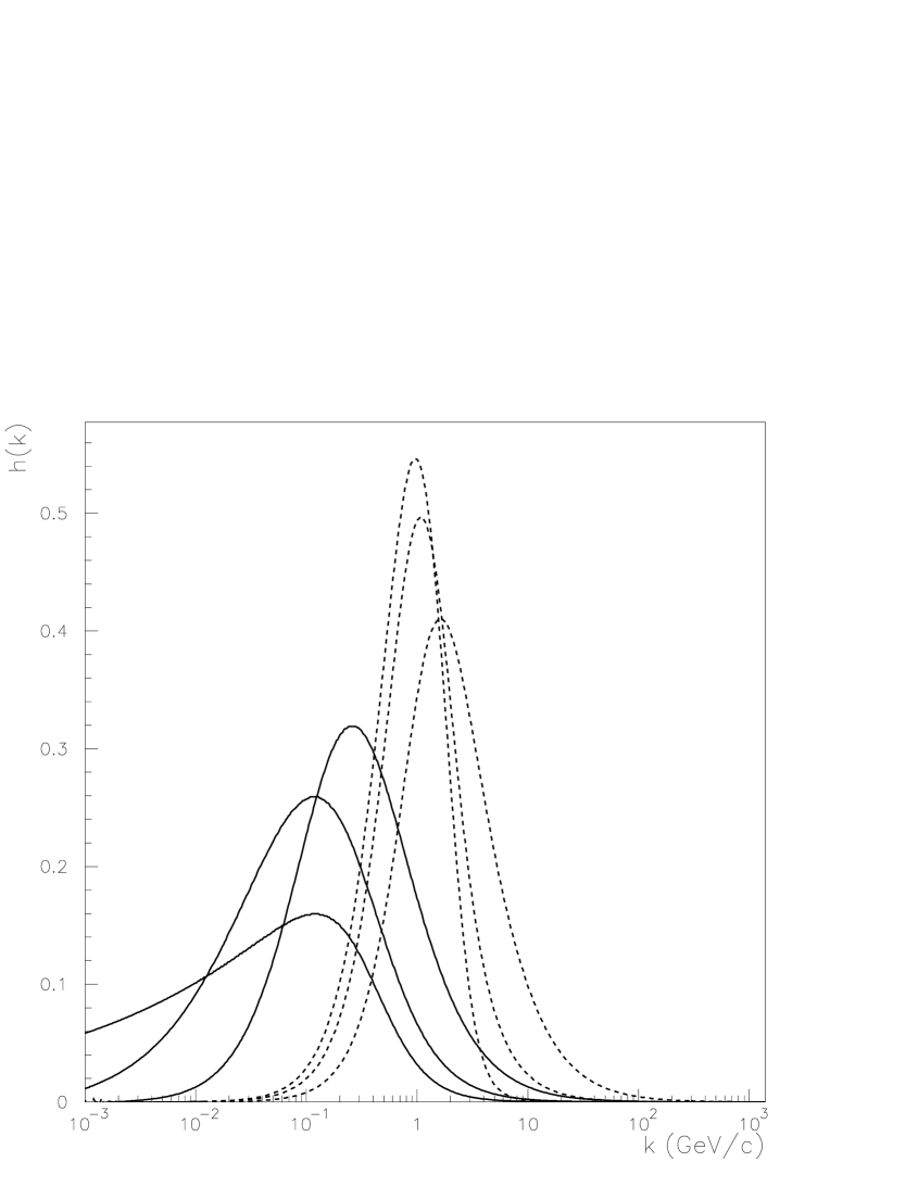
Figure 1:

Figure 2:

Figure 3:

Figure 4:

Figure 5:

Figure 6: