CERN-TH/2001-089
IFT-11/2001
hep-ph/0104034
Nucl. Phys. B611 (2001) 338^⋆

Quark mass effects in $\bar{B}\to X_{s}\gamma$

Paolo Gambino${}^{{}^{1}}$ and Mikołaj Misiak${}^{{}^{1,\,2}}$

${}^{{}^{1}}$Theory Division, CERN, CH-1211 Geneva 23, Switzerland

${}^{{}^{2}}$Institute of Theoretical Physics, Warsaw University,
Hoża 69, PL-00-681 Warsaw, Poland

Abstract

The charm-loop contribution to $\bar{B}\to X_{s}\gamma$ is found to be numerically dominant and very stable under logarithmic QCD corrections. The strong enhancement of the branching ratio by QCD logarithms is mainly due to the $b$-quark mass evolution in the top-quark sector. These observations allow us to achieve better control over residual scale-dependence at the next-to-leading order. Furthermore, we observe that the sensitivity of the matrix element $\langle X_{s}\gamma|(\bar{s}c)_{V-A}(\bar{c}b)_{V-A}|b\rangle$ to $m_{c}/m_{b}$ is the source of a sizeable uncertainty that has not been properly taken into account in previous analyses. Replacing $m_{c}^{\rm pole}/m_{b}^{\rm pole}$ in this matrix element by the more appropriate $m_{c}^{\overline{\rm MS}}(\mu)/m_{b}^{\rm pole}$ with $\mu\in[m_{c},m_{b}]$ causes an 11% enhancement of the SM prediction for BR$[\bar{B}\to X_{s}\gamma]$. For $E_{\gamma}>1.6$ GeV in the $\bar{B}$-meson rest frame, we find BR$[\bar{B}\to X_{s}\gamma]_{E_{\gamma}>1.6~{}{\rm GeV}}=(3.60\pm 0.30)\times 10^{-4}$. The difference between our result and the current experimental world average is consistent with zero at the level of $1\sigma$. We also discuss the implementation of new physics effects in our calculation. The Two–Higgs–Doublet–Model II with a charged Higgs boson lighter than 350 GeV is found to be strongly disfavoured.

                                            
^⋆ Comparison with experiment is updated in the present hep-ph version. In particular, the published results of CLEO [4] are taken into account.

1 Introduction

Strong constraints on new physics from $\bar{B}\to X_{s}\gamma$ [1, 2, 3] crucially depend on theoretical uncertainties in the Standard Model prediction for this decay. This becomes more and more transparent with the progress in experimental accuracy. The current experimental results are

$${\rm BR}[\bar{B}\to X_{s}\gamma] = \left[3.21\pm 0.43_{\rm stat}\pm 0.27_{\rm sys}~{}\left({}^{+0.18}_{-0.10}\right)_{\rm theory}\right]\times 10^{-4}\hskip 48.36967pt\mbox{(CLEO \cite[cite]{[\@@bibref{}{CLEO}{}{}]}),}$$

$${\rm BR}[\bar{B}\to X_{s}\gamma] = \left[3.36\pm 0.53_{\rm stat}\pm 0.42_{\rm sys}\pm 0.54_{\rm theory}\right]\times 10^{-4}\hskip 56.9055pt\mbox{(BELLE \cite[cite]{[\@@bibref{}{BELLE}{}{}]}),}$$

$${\rm BR}[b\to s\gamma] = (3.11\pm 0.80_{\rm stat}\pm 0.72_{\rm sys})\times 10^{-4}\hskip 113.81102pt\mbox{(ALEPH \cite[cite]{[\@@bibref{}{ALEPH}{}{}]}).}$$

The weighted average for BR${}_{\gamma}\equiv$BR$[\bar{B}\to X_{s}\gamma]$ is therefore

$${\rm BR}_{\gamma}^{\rm exp}=(3.23\pm 0.42)\times 10^{-4}$$ (1.1)

with an error of around 13%. Improved results from CLEO and BELLE, as well as new results from BABAR, are expected soon. Thus, all efforts should be made, on the theoretical side, to reduce the uncertainty significantly below 10%.

There are three sources of uncertainties in the theoretical prediction: parametric, non-perturbative and perturbative. The most important parametric ones in our analysis are due to $\alpha_{s}(M_{Z})$ and the HQET parameter $\lambda_{1}$. The latter parameter occurs in the calculation of the phase-space factor of the semileptonic branching ratio that is conventionally used for normalization.

All the non-perturbative effects, except for the calculated $\Lambda^{2}/m_{c,b}^{2}$ corrections [7, 8], sum up to the non-perturbative uncertainty. No satisfactory quantitative estimate of those effects is available, but they are believed to be well below 10% when the photon energy cut–off is above 1 GeV [9] and below 1.9 GeV [10] in the ${\bar{B}}$-meson rest frame. The cut–offs imposed most recently by CLEO and BELLE are 2.0 and 2.1 GeV, respectively, in the $\Upsilon(4S)$ frame.

As far as the perturbative uncertainties are concerned, they were dramatically reduced 4 years ago, after the completion of NLO QCD calculations [11, 12, 13, 14, 15, 16]. A further improvement came from electroweak corrections [10, 17, 18, 19]. The unknown NNLO QCD corrections were estimated at the level of $\pm 7\%$ in ref. [10], where it was pointed out that certain scale-dependence cancellations at NLO seem accidental.

However, one source of perturbative uncertainty was not properly taken into account in the previous analyses [10, 12, 19, 20]. It is related to the question of the definitions of $m_{c}$ and $m_{b}$ that should be used in the matrix element $\langle P_{2}\rangle\equiv\langle X_{s}\gamma|(\bar{s}c)_{V-A}(\bar{c}b)_{V-A}|b\rangle$. This matrix element is non-vanishing at two loops only, so the renormalization scheme for $m_{c}$ and $m_{b}$ is an NNLO issue (unless $\ln\frac{m_{b}}{m_{c}}$ is treated as a large logarithm). However, this problem is numerically very important because of the sensitivity of $\langle P_{2}\rangle$ to $m_{c}/m_{b}$. Changing $m_{c}/m_{b}$ in $\langle P_{2}\rangle$ from  $0.29\pm 0.02$  to  $0.22\pm 0.04$,  i.e. from $m_{c}^{\rm pole}/m_{b}^{\rm pole}$ to $m_{c}^{\overline{\rm MS}}(\mu)/m_{b}^{\rm pole}$ (with $\mu\in[m_{c},m_{b}]$) causes an increase of BR_γ by around 11%. What matters for $\bar{B}\to X_{s}\gamma$ is mainly the real part of $\langle P_{2}\rangle$, where the charm quarks are usually off-shell, with a momentum scale set by $m_{b}^{\rm pole}$ (or some sizeable fraction of it). Therefore, as we shall argue in appendix D, the choice of $m_{c}^{\overline{\rm MS}}(\mu)/m_{b}^{\rm pole}$ with $\mu\in[m_{c},m_{b}]$ seems more reasonable than $m_{c}^{\rm pole}/m_{b}^{\rm pole}$.

Once $m_{c}^{\overline{\rm MS}}(\mu)/m_{b}^{\rm pole}$ with $\mu\in[m_{c},m_{b}]$ is used in $\langle P_{2}\rangle$, the uncertainty in BR_γ significantly increases. This is due in part to a strong scale-dependence of $m_{c}(\mu)$. Moreover, in all the previous analyses, the $m_{c}$-dependence of $\langle P_{2}\rangle$ cancelled partially against that of the semileptonic decay rate. Once the different nature of the charm mass in the two cases is appreciated, the cancellation no longer takes place.

In the present paper, we perform a reanalysis of $\bar{B}\to X_{s}\gamma$, taking the above problems with $m_{c}/m_{b}$ into account. At the same time, we make several improvements in the calculation, which allows us to maintain the theoretical uncertainty at the level of around $\sim\!10\%$. In particular, a careful calculation of the semileptonic phase–space factor is performed, after expressing it in terms of an observable for which the NNLO expressions are known. Moreover, good control over the behaviour of QCD perturbation series in $\bar{B}\to X_{s}\gamma$ is achieved by splitting the charm- and top-quark-loop contributions to the decay amplitude. The overall factor of $m_{b}$ is frozen at the electroweak scale in the top contribution to the effective vertex  $m_{b}(\bar{s}_{L}\sigma^{\mu\nu}b_{R})F_{\mu\nu}$.  All the remaining factors of $m_{b}$ are expressed in terms of the bottom “1S mass”. As argued in ref. [21], expressing the kinematical factors of $m_{b}$ in inclusive $B$-meson decay rates in terms of the 1S mass improves the behaviour of QCD perturbation series with respect to what would be obtained using $m_{b}^{\overline{\rm MS}}(m_{b})$ or $m_{b}^{\rm pole}$. When such an approach is used, no sizeable accidental cancellations of scale-dependence in the NLO expressions for BR_γ are observed any more.

Splitting the charm and top contributions to the amplitude allows us to better understand the origin of the well-known factor of $\;\sim\!\!3$ enhancement of BR_γ by QCD logarithms. When the splitting is performed at LO, the charm contribution is found to be extremely stable under QCD renormalization group evolution. The logarithmic enhancement of the branching ratio appears to be almost entirely due to the top-quark sector. It can be attributed to the large anomalous dimension of the $b$-quark mass.

Our paper is organized as follows. In section 2, splitting of the charm and top contributions is performed at the leading-logarithmic level, and $m_{b}(\mu)$ in the top sector is shown to be the main source of large QCD logarithms. In section 3, the NLO formulae for BR_γ are written in such a way that the NNLO uncertainties can be conveniently controlled. Section 4 is devoted to the numerical analysis, our final result being given in eq. (4.14). In section 5, constraints on new physics are briefly discussed. Section 6 contains our conclusions.

Details on specific points of our calculation as well as the formulae that are necessary to make our analysis self-contained are collected in the appendices. In appendix A, our input parameters are collected. Appendix B is devoted to a determination of the mass ratio $m_{b}^{\overline{MS}}(m_{t})/m_{b}^{1S}$. In appendix C, we calculate the semileptonic phase-space factor. Appendix D contains the determination of the ratio $m_{c}/m_{b}$ that should be used in $\langle P_{2}\rangle$. We also give there the analytical dependence of this matrix element on $m_{c}/m_{b}$  [11]. In appendix E, the relevant bremsstrahlung formulae are summarized.

2 Leading-order considerations

The resummation of large QCD logarithms in $B$ decays usually begins by decoupling the heavy electroweak bosons and the top quark. In the resulting effective theory, flavour-changing interactions are present only in operators $P_{i}$ of dimension$\,>\!4\;$. Their Wilson coefficients $C_{i}(\mu)$ evolve according to the Renormalization Group Equations (RGEs) from the matching scale $\mu_{0}$ down to the scale $\mu_{b}$ where the matrix elements of $P_{i}$ are evaluated.

In the case of $\bar{B}\to X_{s}\gamma$, the relevant operators $P_{i}$ read

$$P_{1} = (\bar{s}_{L}\gamma_{\mu}T^{a}c_{L})(\bar{c}_{L}\gamma^{\mu}T^{a}b_{L}),$$

$$P_{2} = (\bar{s}_{L}\gamma_{\mu}c_{L})(\bar{c}_{L}\gamma^{\mu}b_{L}),$$

$$P_{3} = (\bar{s}_{L}\gamma_{\mu}b_{L})\sum_{q}(\bar{q}\gamma^{\mu}q),$$

$$P_{4} = (\bar{s}_{L}\gamma_{\mu}T^{a}b_{L})\sum_{q}(\bar{q}\gamma^{\mu}T^{a}q),$$

$$P_{5} = (\bar{s}_{L}\gamma_{\mu}\gamma_{\nu}\gamma_{\rho}b_{L})\sum_{q}(\bar{q}\gamma^{\mu}\gamma^{\nu}\gamma^{\rho}q),$$

$$P_{6} = (\bar{s}_{L}\gamma_{\mu}\gamma_{\nu}\gamma_{\rho}T^{a}b_{L})\sum_{q}(\bar{q}\gamma^{\mu}\gamma^{\nu}\gamma^{\rho}T^{a}q),$$

$$P_{7} = \frac{e}{16\pi^{2}}m_{b}(\mu)(\bar{s}_{L}\sigma^{\mu\nu}b_{R})F_{\mu\nu},$$

$$P_{8} = \frac{g}{16\pi^{2}}m_{b}(\mu)(\bar{s}_{L}\sigma^{\mu\nu}T^{a}b_{R})G_{\mu\nu}^{a}.$$ (2.1)

In the leading logarithmic approximation, the $b\to s\gamma$ amplitude is proportional to the (effective) Wilson coefficient of the operator $P_{7}$. The well-known [22] expression for this coefficient reads

$$C^{(0)\rm eff}_{7}(\mu_{b})=\eta^{\frac{16}{23}}C^{(0)}_{7}(\mu_{0})+\frac{8}{3}\left(\eta^{\frac{14}{23}}-\eta^{\frac{16}{23}}\right)C^{(0)}_{8}(\mu_{0})+\sum_{i=1}^{8}h_{i}\eta^{a_{i}},$$ (2.2)

where $\eta=\alpha_{s}(\mu_{0})/\alpha_{s}(\mu_{b})$ and

$$h_{i}=\left(\begin{array}[]{cccccccc}\frac{626126}{272277}&-\frac{56281}{51730}&-\frac{3}{7}&-\frac{1}{14}&-0.6494&-0.0380&-0.0185&-0.0057\end{array}\right).$$ (2.3)

The powers $a_{i}$ are given in table 1, in section 3. The coefficients $C^{(0)}_{7}(\mu_{0})$ and $C^{(0)}_{8}(\mu_{0})$ are found from the one-loop electroweak diagrams presented in fig. 1. It is sufficient to calculate the 1PI diagrams only.

$\gamma$                                  $\gamma$                                      $\gamma$                                  $\gamma$
$u,c,t$          $u,c,t$             $W^{\pm}$         $W^{\pm}$               $u,c,t$          $u,c,t$              $G^{\pm}$         $G^{\pm}$
         
$b$           $W^{\pm}$        $s$        $b$        $u,c,t$        $s$            $b$           $G^{\pm}$         $s$        $b$        $u,c,t$        $s$

Figure 1: One-loop 1PI diagrams for $b\to s\gamma$ in the SM. There is no $W^{\pm}G^{\mp}\gamma$ coupling in the background-field gauge.

Contributions from different internal quark flavours in those diagrams can be separately matched onto gauge-invariant operators, even when the calculation is performed off-shell. For the operator $P_{7}$ and its gluonic analogue $P_{8}$, each quark flavour yields a UV-finite contribution that depends neither on the renormalization scheme nor on the gauge-fixing parameter.

When such a separation of flavours is made, and the CKM-suppressed $u$-quark contribution is neglected, eq. (2.2) can be written as

$$C^{(0)\rm eff}_{7}(\mu_{b})=X_{c}+X_{t},$$ (2.4)

where the charm-quark contribution is given by

$$X_{c}\;=\;-\frac{23}{36}\eta^{\frac{16}{23}}-\frac{8}{9}\left(\eta^{\frac{14}{23}}-\eta^{\frac{16}{23}}\right)+\sum_{i=1}^{8}h_{i}\eta^{a_{i}},$$ (2.5)

and the top-quark one reads

$$X_{t}\;=\;-\frac{1}{2}A_{0}^{t}\left(\frac{m_{t}^{2}}{M_{W}^{2}}\right)\eta^{\frac{16}{23}}-\frac{4}{3}F_{0}^{t}\left(\frac{m_{t}^{2}}{M_{W}^{2}}\right)\left(\eta^{\frac{14}{23}}-\eta^{\frac{16}{23}}\right),$$ (2.6)

where

$$\begin{array}[]{rcl}A^{t}_{0}(x)&=&\frac{-3x^{3}+2x^{2}}{2(x-1)^{4}}\ln x+\frac{-22x^{3}+153x^{2}-159x+46}{36(x-1)^{3}},\\[8.53581pt] F^{t}_{0}(x)&=&\frac{3x^{2}}{2(x-1)^{4}}\ln x+\frac{-5x^{3}+9x^{2}-30x+8}{12(x-1)^{3}}.\\[-8.53581pt] \end{array}$$

The first two terms in $X_{c}$ (2.5) are obtained from eq. (2.2) by the following replacements:

$C^{(0)}_{7}(\mu_{0})\to-\frac{23}{36}$ and $C^{(0)}_{8}(\mu_{0})\to-\frac{1}{3}$, which is equivalent to including only charm contributions to the matching conditions for the corresponding operators. Analogously, only top loops contribute to $X_{t}$. The last term in eq. (2.2) now appears in $X_{c}$, because it is entirely due to effects of charm loops in the RGE evolution. The splitting of charm and top is performed at the level of SM Feynman diagrams, and the effective theory is nothing but a technical tool for resumming large QCD logarithms in gluonic corrections to those diagrams.

$\eta$

Figure 2: $X_{c}$ as a function of $\eta$ (solid line), and its three components in eq. (2.5) (dashed lines).

$X_{c}$ is a function of $\eta$ that varies very slowly in the physically interesting region $0.4<\eta<1$. This is illustrated in fig. 2, where the three components of $X_{c}$ in eq. (2.5) are plotted as well. The second component is numerically small, while there is a strong cancellation of the $\eta$-dependence between the first and the third component. However, these components are not separately physical in any conceivable limit, so the cancellation cannot be considered accidental.

Since $X_{c}$ is practically scale-independent, $X_{t}$ must be the source of the factor of $\;\sim\!\!3$ enhancement of BR_γ by QCD logarithms. This is indeed the case, because all the powers of $\eta$ in eq. (2.6) are positive and quite large. When $\eta$ changes from unity to 0.566 (which corresponds to $\mu_{0}=M_{W}$ and $\mu_{b}=5$ GeV), then $X_{t}$ decreases from 0.450 to 0.325. At the same time, $X_{c}$ changes by only 0.008 (from $-\frac{23}{36}\approx-0.639$ to $-0.631$). Consequently, $|C^{(0)\rm eff}_{7}(\mu)|^{2}$ increases from 0.036 to 0.094, i.e. the branching ratio gets enhanced by a factor of 2.6.

It is easy to identify the reason for the strong $\eta$-dependence of $X_{t}$. It is the large anomalous dimension of $m_{b}(\mu)$ that stands in front of the operator $P_{7}$ (2.1). The anomalous dimension $\gamma_{m}$ is responsible for $\frac{12}{23}$ out of $\frac{16}{23}$ in the power of $\eta$ that multiplies the (numerically dominant) function $A_{0}^{t}(x)$ in the expression for $X_{t}$. Thus, the logarithmic QCD effects in $b\to s\gamma$ can be approximately taken into account by simply keeping $m_{b}$ renormalized at $\mu_{0}\sim(m_{t}$ or $M_{W})$ in the top contribution to the decay amplitude. In section 4, we shall see that those features carry on at the NLO, lending support to the idea that they are not due to a numerical coincidence, and remain valid at the NNLO, too.

It would be interesting to understand the physics behind the different optimal normalizations of $m_{b}$ in the charm and top loops. In this respect, the following observations may be helpful. Off–shell $b\to s\gamma$ and $b\to s\;gluon$ diagrams mediated by charm loops give rise only to dimension-six operators $P_{\sigma FD}=\frac{ie}{16\pi^{2}}\bar{s}_{L}\{\sigma_{\mu\nu}F^{\nu\mu},D\hskip-8.55695pt\lower-0.91666pt\hbox to8.55695pt{\hss\sl/\/\hss}\}b_{L}$  and  $P_{\sigma GD}=\frac{ig}{16\pi^{2}}\bar{s}_{L}\{\sigma_{\mu\nu}G^{a\;\nu\mu}T^{a},D\hskip-8.55695pt\lower-0.91666pt\hbox to8.55695pt{\hss\sl/\/\hss}\}b_{L}$, respectively. The basis of physical operators in the off-shell effective theory for the charm sector can be chosen to be $\{P_{1},...,P_{6},P_{\sigma FD},P_{\sigma GD}\}$. The LO Wilson coefficient of $P_{\sigma FD}$ is given by eq. (2.5), i.e. its RGE evolution is very slow. When the evolution is terminated at $\mu_{b}$, and the equations of motion (EOM) are used afterwards, $P_{\sigma FD}$ reduces to the operator $P_{7}$ that contains an overall factor of $m_{b}$. Thus, the $b$ mass naturally associated with charm loops is a low energy, low virtuality mass.

Figure 3: Chirality flows in diagrams contributing to $C_{7}^{(0)}(\mu_{0})$. The photon couples to any of the internal lines.

In the top loops, on the other hand, $m_{b}$ appears in two ways: either through the same mechanism as in the charm loops (fig. 3a,b), or via the bottom Yukawa coupling $y_{b}$ of a right-handed $b$ with a left-handed top quark (fig. 3c). In the first case, the RGE evolution of $C^{t}_{\sigma FD}(\mu)$ and $C^{t}_{\sigma GD}(\mu)$ is much faster than in the charm sector. Such a fast running can be compensated to a large extent by using $m_{b}(\mu_{0})$ in the EOM at the low–energy scale. In the second case, it is not necessary to use the EOM to project on $P_{7}$. The natural normalization scale of the Yukawa coupling $y_{b}(\mu)$ is given by the heavy masses circulating in the loop. The $b$ mass associated with the Yukawa contributions is therefore a high–energy mass, $m_{b}(\mu_{0})$ with $\mu_{0}\sim(M_{W}~{}{\rm or}~{}m_{t})$. This reasoning leads us to the conclusion that the appropriate normalization of the total top contribution is in terms of $m_{b}(\mu_{0})$.

A careful reader might worry about how this picture can be reconciled with GIM cancellations that take place in the case of degenerate quarks. Some light on this issue can be shed by considering a hypothetical situation when $m_{b}\ll m_{c}\ll m_{t}\ll M_{W}$. In such a case, the effective $bs\gamma$ interaction would be relatively well approximated by

$${\cal L}_{\rm int}\approx\frac{4G_{F}}{\sqrt{2}}V^{*}_{ts}V_{tb}\left\{\frac{23}{36}[m_{b}(m_{t})-m_{b}(m_{c})]+{\cal O}(m^{2}_{c,t}/M_{W}^{2})\right\}\bar{s}_{L}\sigma^{\mu\nu}b_{R}F_{\mu\nu}.$$ (2.7)

It is not an exact formula even at LO, because we have neglected the very slow RGE running from $M_{W}$ to $m_{c,t}$ and the small anomalous dimensions of $P_{7,8}/m_{b}(\mu)$. However, eq. (2.7) works numerically quite well. The QCD enhancement of BR_γ can be much larger here (than in the real world), and its main reason is clearly seen. The number $\frac{23}{36}$ arises from the matching condition with an effectively massless internal quark. In the absence of QCD, it drops out owing to GIM cancellation. However, no cancellation takes place any longer when the QCD evolution of $m_{b}$ is taken into account.

3 Next-to-leading order formulae

We have seen in the previous section that most of the leading QCD logarithms can be taken into account by keeping the top and charm contributions split, and by renormalizing $m_{b}(\mu)$ in $P_{7}$ (2.1) at $\mu_{0}\sim(m_{t}$ or $M_{W})$ in the top contribution to the decay amplitude. Motivated by this observation, we shall now rewrite the known NLO expressions for $\bar{B}\to X_{s}\gamma$ in an analogous manner. As we shall see, this simple operation not only allows us to reproduce the logarithmic QCD enhancement in a satisfactory manner, but also the NLO corrections become significantly smaller than in the traditional approach. Moreover, the residual renormalization-scale-dependence diminishes, without any accidental cancellations involved. In other words, the behaviour of QCD perturbation series improves.

Assuming that the dominant NNLO QCD effects have the same origin as the dominant LO and NLO ones, we shall use all the currently known perturbative information to determine the ratio of $m_{b}(\mu_{0})$ to the low–energy $b$-quark mass that normalizes the semileptonic decay rate. This low–energy mass will be chosen in a manner that ensures good convergence of QCD-perturbation series for the semileptonic decay.

Our input here are the standard NLO QCD formulae for $B\to X_{s}\gamma$ collected in ref. [12], and the separate charm-sector and top-sector matching conditions for the relevant operators presented in section 2 of ref. [23]. The evaluation of such separate matching conditions was described in great detail in section 5 of the latter paper. We have also checked it independently with the method of ref. [1]. Apart from the perturbative QCD effects, we shall include the electroweak and the available non-perturbative corrections.

The $\bar{B}\to X_{s}\gamma$ branching ratio with an energy cut–off $E_{0}$ in the $\bar{B}$-meson rest frame can be expressed as follows:

$${\rm BR}[\bar{B}\to X_{s}\gamma]^{{\rm subtracted~{}}\psi,\;\psi^{\prime}}_{E_{\gamma}>E_{0}}={\rm BR}[\bar{B}\to X_{c}e\bar{\nu}]_{\rm exp}\left|\frac{V^{*}_{ts}V_{tb}}{V_{cb}}\right|^{2}\frac{6\alpha_{\rm em}}{\pi\;C}\left[P(E_{0})+N(E_{0})\right],$$ (3.1)

where $\alpha_{\rm em}=\alpha_{\rm em}^{\rm on~{}shell}$ [17] and $P(E_{0})$ is given by the perturbative ratio

$$\frac{\Gamma[b\to X_{s}\gamma]_{E_{\gamma}>E_{0}}}{|V_{cb}/V_{ub}|^{2}\;\Gamma[b\to X_{u}e\bar{\nu}]}=\left|\frac{V^{*}_{ts}V_{tb}}{V_{cb}}\right|^{2}\frac{6\alpha_{\rm em}}{\pi}\;P(E_{0}).$$ (3.2)

$N(E_{0})$ denotes the non-perturbative correction. Contrary to the standard approach, we have chosen the charmless semileptonic rate (corrected for the appropriate CKM angles) to be the normalization factor in eq. (3.2). This modification is offset by the factor $C$ in eq. (3.1):

$$C=\left|\frac{V_{ub}}{V_{cb}}\right|^{2}\frac{\Gamma[\bar{B}\to X_{c}e\bar{\nu}]}{\Gamma[\bar{B}\to X_{u}e\bar{\nu}]}.$$ (3.3)

This observable can either be measured or calculated. Our normalization to the charmless semileptonic rate in the l.h.s. of eq. (3.2) is motivated by the need for separating the problem of $m_{c}$ determination from the problem of convergence of perturbation series in $b\to X_{s}\gamma$. The factor $C$ can be called “the non-perturbative semileptonic phase-space factor”.

The superscript “subtracted $\psi$ and $\psi^{\prime}$” on the l.h.s. of eq. (3.1) means that the processes

$$\bar{B} \to \psi^{(}{}^{\prime}{}^{)}X^{(1)}$$ (3.4)

$$\hskip 8.53581pt\searrow$$

$$\hskip 19.91692ptX^{(2)}\gamma$$

are treated as background, and should be subtracted on the experimental side. This background is negligible (below 1%) for a cut–off of 2.1 GeV on the photon energy in the $\bar{B}$-meson rest frame, but may have a $\sim 5\%$ effect when the cut–off is lowered to 1.8 GeV.

The perturbative quantity $P(E_{0})$ can be written in the following form:

$$P(E_{0})=\left|K_{c}+\left(1+\frac{\alpha_{s}(\mu_{0})}{\pi}\ln\frac{\mu_{0}^{2}}{m_{t}^{2}}\right)r(\mu_{0})K_{t}+\varepsilon_{\rm ew}\right|^{2}+B(E_{0}),$$ (3.5)

where $K_{t}$ contains the top contributions to the $b\to s\gamma$ amplitude. $K_{c}$ contains the remaining contributions, among which the charm loops are by far dominant. The electroweak correction to the $b\to s\gamma$ amplitude is denoted by $\varepsilon_{\rm ew}$. The ratio

$$r(\mu_{0})=\frac{m_{b}^{\overline{\rm MS}}(\mu_{0})}{m_{b}^{1S}}$$ (3.6)

appears in eq. (3.5) because we keep $m_{b}$ renormalized at $\mu_{0}$ in the top contribution to the operator $P_{7}$ (2.1), while all the kinematical factors of $m_{b}$ are expressed in terms of the bottom “1S mass”. The 1S mass is defined as half of the perturbative contribution to the $\Upsilon$ mass. As argued in ref. [21], expressing the kinematical factors of $m_{b}$ in inclusive $B$-meson decay rates in terms of the 1S mass improves the behaviour of QCD perturbation series with respect to what would be obtained using $m_{b}^{\overline{\rm MS}}(m_{b})$ or $m_{b}^{\rm pole}$.

The bremsstrahlung function $B(E_{0})$ contains the effects of $b\to s\gamma g$ and $b\to s\gamma q\bar{q}$ $(q=u,d,s)$ transitions. It is the only $E_{0}$-dependent part in $P(E_{0})$. It is given in appendix E. Its influence on the $b\to X_{s}\gamma$ branching ratio is less than 4% when $1~{}{\rm GeV}<E_{0}<2~{}{\rm GeV}$. Therefore, we do not split the top and charm contributions to this function. It would not improve the overall accuracy at all, but only make the formulae unnecessarily complicated.

$k$	1	2	3	4	5	6	7	8
$a_{k}$	$\frac{14}{23}$	$\frac{16}{23}$	$\frac{6}{23}$	$-\frac{12}{23}$	0.4086	$-$0.4230	$-$0.8994	0.1456
$d_{k}$	1.4107	$-$0.8380	$-$0.4286	$-$0.0714	$-$0.6494	$-$0.0380	$-$0.0185	$-$0.0057
$\tilde{d}_{k}$	$-$17.6507	11.3460	3.5762	$-$2.2672	3.9267	1.1366	$-$0.5445	0.1653
$\tilde{d}^{\eta}_{k}$	9.2746	$-$6.9366	$-$0.8740	0.4218	$-$2.7231	0.4083	0.1465	0.0205
$\tilde{d}^{a}_{k}$	0	0	1	1	0	0	0	0
$\tilde{d}^{b}_{k}$	0	0	1	1	0	0	0	0
$\tilde{d}^{i\pi}_{k}$	0.4702	0	$-$0.4938	$-$0.4938	$-$0.8120	0.0776	$-$0.0507	0.0186
$e_{k}$	5.2620	$-$3.8412	0	0	$-$1.9043	$-$0.1008	0.1216	0.0183

Table 1: “Magic numbers” for $K_{c}$ and $K_{t}$

Our result for $K_{c}$ reads

$$K_{c} = \sum_{k=1}^{8}\eta^{a_{k}}\left\{d_{k}+\frac{\alpha_{s}(\mu_{b})}{4\pi}\left[2\beta_{0}a_{k}d_{k}\left(\ln\frac{m_{b}}{\mu_{b}}+\eta\ln\frac{\mu_{0}}{M_{W}}\right)\right.\right.$$ (3.7)

$$\left.\left.+\tilde{d}_{k}+\tilde{d}^{\eta}_{k}\;\eta+\tilde{d}^{a}_{k}a(z)+\tilde{d}^{b}_{k}b(z)+\tilde{d}^{i\pi}_{k}i\pi\right]\right\}\;\;+\frac{V_{us}^{*}V_{ub}}{V_{ts}^{*}V_{tb}}\,\frac{\alpha_{s}}{4\pi}\,\left(\eta^{a_{3}}+\eta^{a_{4}}\right)[a(z)+b(z)],$$

where $\beta_{0}=\frac{23}{3}$ and $z=(m_{c}/m_{b})^{2}$. The functions $a(z)$ and $b(z)$ are given in appendix D.

The “magic numbers” $d_{k},~{}\tilde{d}_{k},~{}...$ can be found in table 1. In their evaluation, the unknown NLO matrix elements $r_{3},...,r_{6}$ [12] have been set to zero. The resulting error will be absorbed in the NNLO uncertainty below. This is mandatory because   $C^{(0)}_{k}(\mu_{b})/C^{(0)}_{2}(\mu_{b})\leq\frac{\alpha_{s}(\mu_{b})}{\pi}$  for  $k=3,...,6$.

The NLO expression for $K_{t}$ is as follows

$$K_{t} = \left[1-\frac{2}{9}\alpha_{s}(m_{b})^{2}+\frac{\alpha_{s}(\mu_{0})}{\pi}\ln\frac{\mu_{0}}{m_{t}}\;\;4x\frac{\partial}{\partial x}\right]\left[-\frac{1}{2}\eta^{\frac{4}{23}}A^{t}_{0}(x)+\frac{4}{3}\left(\eta^{\frac{4}{23}}-\eta^{\frac{2}{23}}\right)F^{t}_{0}(x)\right]$$

$$+\frac{\alpha_{s}(\mu_{b})}{4\pi}\left\{E_{0}^{t}(x)\sum_{k=1}^{8}e_{k}\eta^{\left(a_{k}+\frac{11}{23}\right)}\right.$$

$$\left.+\eta^{\frac{4}{23}}\left[-\frac{1}{2}\eta A^{t}_{1}(x)+\left(\frac{12523}{3174}~{}~{}-\frac{7411}{4761}\eta~{}~{}~{}~{}-\frac{2}{9}\pi^{2}~{}~{}-\frac{4}{3}~{}\left(\ln\frac{m_{b}}{\mu_{b}}+\eta\ln\frac{\mu_{0}}{m_{t}}\right)\right)A^{t}_{0}(x)\right.\right.$$

$$\left.\left.\hskip 17.07164pt+\frac{4}{3}\eta F^{t}_{1}(x)+\left(-\frac{50092}{4761}+\frac{1110842}{357075}\eta+\frac{16}{27}\pi^{2}+\frac{32}{9}\left(\ln\frac{m_{b}}{\mu_{b}}+\eta\ln\frac{\mu_{0}}{m_{t}}\right)\right)F^{t}_{0}(x)\right]\right.$$

$$\left.+\eta^{\frac{2}{23}}\left[-\frac{4}{3}\eta F^{t}_{1}(x)+\left(\frac{2745458}{357075}-\frac{38890}{14283}\eta-\frac{4}{9}\pi(\pi+i)-\frac{16}{9}\left(\ln\frac{m_{b}}{\mu_{b}}+\eta\ln\frac{\mu_{0}}{m_{t}}\right)\right)F^{t}_{0}(x)\right]\right\}.$$

The functions $A^{t}_{0}$ and $F^{t}_{0}$ of $x=(m_{t}(\mu_{0})/M_{W})^{2}$ have already been given in eq. (2). The remaining functions read

$$\begin{array}[]{rcl}E^{t}_{0}(x)&=&\frac{-9x^{2}+16x-4}{6(x-1)^{4}}\ln x+\frac{7x^{3}+21x^{2}-42x-4}{36(x-1)^{3}},\\[5.69054pt] A^{t}_{1}(x)&=&\frac{32x^{4}+244x^{3}-160x^{2}+16x}{9(1-x)^{4}}Li_{2}\left(1-\frac{1}{x}\right)+\frac{-774x^{4}-2826x^{3}+1994x^{2}-130x+8}{81(1-x)^{5}}\ln x\\[11.38109pt] &&+\frac{-94x^{4}-18665x^{3}+20682x^{2}-9113x+2006}{243(1-x)^{4}},\\[5.69054pt] F^{t}_{1}(x)&=&\frac{4x^{4}-40x^{3}-41x^{2}-x}{3(1-x)^{4}}Li_{2}\left(1-\frac{1}{x}\right)+\frac{-144x^{4}+3177x^{3}+3661x^{2}+250x-32}{108(1-x)^{5}}\ln x\\[11.38109pt] &&+\frac{-247x^{4}+11890x^{3}+31779x^{2}-2966x+1016}{648(1-x)^{4}}.\end{array}$$ (3.14)

The ${\cal O}(\alpha_{s}^{2})$ term is included in $K_{t}$ along the lines of the $\Upsilon$ expansion [21]. Its effect is at the level of 1% only, and it is offset by an analogous term in $r$ (3.6) (see appendix B).

The electroweak correction $\varepsilon_{\rm ew}$ in eq. (3.5) consists of three terms

$$\varepsilon_{\rm ew}=\delta^{\rm ew}C_{7}^{(0)\rm eff}(\mu_{b})+\frac{\alpha_{em}(M_{Z})}{\alpha_{s}(\mu_{b})}C_{7}^{\rm em(0)eff}(\mu_{b})-\frac{\alpha_{em}(M_{Z})}{\pi}\left(K_{c}^{(0)}+rK_{t}^{(0)}\right)\ln\frac{M_{Z}}{\mu_{b}}.$$ (3.15)

The first term stands for the dominant non–logarithmic electroweak effects calculated in ref. [19] (see eq. (11) of that paper). The remaining two terms originate from the logarithmically enhanced electromagnetic corrections to the weak radiative (eq. (12) of ref. [18]) and semileptonic (eq. (1) of ref. [24]) decays, respectively. In the last term, $K_{c}^{(0)}$ and $K_{t}^{(0)}$ are just the LO contributions to $K_{c}$ and $K_{t}$.

The non-perturbative correction $N(E_{0})$ in eq. (3.1) is partly known

$$N(E_{0})=-\frac{1}{18}\left(K_{c}^{(0)}+rK_{t}^{(0)}\right)\left(\eta^{\frac{6}{23}}+\eta^{-\frac{12}{23}}\right)\;\frac{\lambda_{2}}{m_{c}^{2}}+...$$ (3.16)

The calculable $\Lambda^{2}/m_{c}^{2}$ correction [7] is taken into account above, while the calculable $\Lambda^{2}/m_{b}^{2}$ corrections [8] have cancelled out because of our normalization to the charmless semileptonic rate. The dots stand for higher-order terms in the heavy-quark expansion [7, 25], as well as for the non-perturbative effects due to higher (than $\psi$ and $\psi^{\prime}$) intermediate $\bar{c}c$ states, to light-quark loops and to motion of the $b$-quark inside the $\bar{B}$ meson. In our numerical results (calculated with $E_{0}=1.6$ GeV), we shall set those effects to zero without including any additional uncertainty.

4 Numerical analysis

In the present section, we shall test our formulae numerically. The experimental inputs and the ranges for the renormalization scales are collected in appendix A. Appendices B, C and D are devoted to the determination of the mass ratio $r$ (3.6), the phase-space factor C (3.3) and the $z$-dependent terms in $K_{c}$ (3.7), respectively. The final results obtained there read

$$r(\mu_{0}=m_{t}) = 0.578\pm 0.002_{\mu_{b}}\pm(\mbox{parametric errors})$$ (4.1)

$$C = 0.575\;(1\pm 0.01\pm 0.02\pm 0.02)$$ (4.2)

$$a(z) = (0.97\pm 0.25)\;+\;i(1.01\pm 0.15)$$ (4.3)

$$b(z) = (-0.04\pm 0.01)\;+\;i(0.09\pm 0.02).$$ (4.4)

In our NLO computation, the imaginary parts of $K_{c}$ and $K_{t}$ are irrelevant, because all the ${\cal O}(\alpha_{s}^{2})$ terms on the r.h.s. of eq. (3.5) are set to zero after the square is taken. If the imaginary parts of $K_{c}$ and $K_{t}$ were not set to zero, they would affect $P(E_{0})$ by only 0.5%.

The ratio of CKM angles standing in front of $P(E_{0})$ can be expressed in terms of the Wolfenstein parameters as follows

$$\left|\frac{V^{*}_{ts}V_{tb}}{V_{cb}}\right|^{2} = 1+\lambda^{2}(2\bar{\rho}-1)+\lambda^{4}(\bar{\rho}^{2}+\bar{\eta}^{2}-A^{2})+{\cal O}(\lambda^{6})$$ (4.5)

$$\approx 0.971+0.10(\bar{\rho}-0.224)=0.971\pm 0.004,$$

where we have used $\lambda=0.2237$, $A=0.819$, $\bar{\rho}=0.224\pm 0.038$ and $\bar{\eta}=0.317$  [26]. The only relevant source of uncertainty is the error in ${\bar{\rho}}$. Even if this error were enlarged by a factor of 2, the influence of $|V^{*}_{ts}V_{tb}/V_{cb}|^{2}$ on the overall uncertainty in $\bar{B}\to X_{s}\gamma$ would remain negligible. The central value of eq. (4.5) is also consistent with the analysis of ref. [27].

The electroweak and non-perturbative corrections from eqs. (3.15) and (3.16) take the following values

$$\varepsilon_{\rm ew} \approx 0.0035+0.0012+0.0028=0.0075$$ (4.6)

$$N(E_{0}) = 0.0036\pm 0.0006\,.$$ (4.7)

Their effects on BR_γ are $-3.8\%$ and $+2.5\%$, respectively. In the electroweak correction, $M_{\rm Higgs}=115$ GeV has been used. The sensitivity of our final result (4.14) to $M_{\rm Higgs}$ is very weak (only 0.3% when $M_{\rm Higgs}$ changes from 115 GeV to 200 GeV). In $N(E_{0})$, $\lambda_{2}=0.12~{}{\rm GeV}^{2}$ and $m_{c}=m_{c}(m_{c})=(1.25\pm 0.10)$ GeV [29] have been used. The indicated uncertainty is due to $m_{c}$ only.

In the “naive” approach, when only the one–loop electroweak diagrams are calculated, one finds

$$K_{c}^{\rm naive}=-\frac{23}{36}\approx-0.639\hskip 28.45274pt{\rm and}\hskip 28.45274ptK_{t}^{\rm naive}=-\frac{1}{2}A^{t}_{0}(x)\approx 0.450.$$ (4.8)

From those numbers, we obtain

$$K_{c}^{\rm naive}+\frac{m_{b}(m_{t})}{m_{b}^{1S}}K_{t}^{\rm naive}\approx-0.379,$$ (4.9)

which implies BR${}^{\rm naive}_{\gamma}\approx 3.53\times 10^{-4}$  (for $N(E_{0})=0$). If the factor $m_{b}(m_{t})/m_{b}^{1S}$ were not included, our “naive” prediction would be 4 times lower.

At LO, i.e. when the ${\cal O}(\alpha_{s})$ terms in eqs. (3.7) and (LABEL:Kt) are neglected, we find

$$K_{c}^{(0)}=-0.631^{-0.003}_{+0.000}\hskip 28.45274pt{\rm and}\hskip 28.45274ptK_{t}^{(0)}=0.434^{-0.005}_{+0.004},$$ (4.10)

which implies that BR${}_{\gamma}^{\rm LO}=3.56^{+0.14}_{-0.07}\times 10^{-4}$. The indicated errors correspond to the variation of the low-energy scale $\mu_{b}$, as described in appendix A.

At NLO, we find for $E_{0}=1.6$ GeV

$$K_{c} = -0.611^{+0.002}_{-0.001}+i\;\left(-0.032^{-0.009}_{+0.006}\right),$$ (4.11)

$$K_{t} = \hskip 8.53581pt(0.397\pm 0.003)+i\;(0.011\pm 0.002),$$ (4.12)

$$B(E_{0}) = 3.1^{+1.3}_{-0.7}\times 10^{-3}.$$ (4.13)

From the above three results, we obtain BR$[\bar{B}\to X_{s}\gamma]_{E_{\gamma}>1.6~{}{\rm GeV}}=3.60^{+0.04}_{-0.05}\times 10^{-4}$. As before, the quoted errors are due to $\mu_{b}$ only.

We can see that the $\mu_{b}$-dependence of ${\rm Re}(K_{c})$ and ${\rm Re}(K_{t})$ is very weak, both at LO and at NLO. Such a weak scale-dependence is somewhat surprising at LO, but at NLO it is not. Moreover, at NLO, the weak scale-dependence is not a result of any accidental cancellation among strongly $\mu_{b}$-dependent terms. Whatever cancellations occur, they occur inside the charm contribution $K_{c}$, and thus cannot be considered accidental.

Since the $\mu_{b}$-dependence of the NLO branching ratio is very weak (below $\pm 1.4\%$), and the dependence on $\mu_{0}$ is not stronger, we can estimate the NNLO corrections by simply saying that they are of order $(\alpha_{s}(m_{b})/\pi)^{2}\approx 0.5\%$, up to an unknown factor of order unity. Thus, it seems safe to assume a value of $\pm 4\%$ for the theoretical error which is due to neglecting $r_{3}$, …, $r_{6}$ at NLO and to the NNLO effects. This is almost twice the combined scale-dependence of the result obtained by scanning $\mu_{b}$ and $\mu_{0}$ between one half and twice their central values (2.2%). We consider the error related to the value of $m_{c}/m_{b}$ in $K_{c}$ separately. The latter uncertainty amounts to $\pm 5.5\%$ alone, when our estimate from appendix D is used.

When all the sources of uncertainties are included, we find

$${\rm BR}[\bar{B}\to X_{s}\gamma]^{{\rm subtracted~{}}\psi,\;\psi^{\prime}}_{E_{\gamma}>1.6~{}{\rm GeV}} = 3.60\times 10^{-4}\;(1\pm 0.06_{(m_{c}/m_{b}~{}{\rm in}~{}K_{c})}\pm 0.04_{\rm(other~{}NNLO)}$$ (4.14)

$$\hskip 76.82243pt\pm 0.01_{\rm(pert~{}C)}\pm 0.02_{\rm\lambda_{1}}\pm 0.02_{\rm\Delta}$$

$$\hskip 76.82243pt\pm 0.02_{\alpha_{s}(M_{Z})}\pm 0.02_{{\rm BR}({\rm semilept})_{\rm exp}}\pm 0.01_{m_{t}})$$

$$= (3.60\pm 0.30)\times 10^{-4}.$$

The errors in the second line above originate from the semileptonic phase-space factor in eq. (C.13). The last of them is due to the error in $m_{b}^{1S}$. Other effects caused by the uncertainty in $m_{b}^{1S}$ are negligible (below 0.2%).

In the last line of eq. (4.14), all the uncertainties have been added in squares. Thus, the final error has only an illustrative character, because many of the partial ones have no statistical interpretation.

We have chosen $E_{0}=1.6$ GeV instead of the commonly used $E_{0}=\frac{1}{20}m_{b}\approx 0.23$ GeV (i.e. $\delta\equiv 1-2E_{0}/m_{b}=0.9$), because the low-energy photons in $\bar{B}\to X_{s}\gamma$ are not experimentally accessible. For high values of the cut–off (around and above 2 GeV), non-perturbative uncertainties are much larger because the $\bar{B}$–meson shape functions are unknown. Models for the shape functions considered in refs. [10, 30] suggest that $E_{0}=1.6$ GeV is already low enough to make those uncertainties negligible. In our opinion, the way to resolve this issue is to measure the photon spectrum without any theoretical input, with the photon energy cut–off as low as possible (e.g. 2.0 or 1.9 GeV in the $\bar{B}$–meson rest frame). Next, a simple extrapolation to the theoretically known spectrum in the vicinity of 1.6–1.7 GeV should be made. For this purpose, the following approximate expression for the integrated branching ratio as a function of $E_{0}$ might be useful:

$$BR(E_{0})=(3.524+0.298E_{0}-0.157E_{0}^{2})\times 10^{-4},$$ (4.15)

where $E_{0}$ is expressed in GeV. The above expression has been obtained as a fit to our results in the region 1 GeV $<E_{0}<$ 2 GeV. The accuracy of this fit is $\pm 0.3\%$. Outside the considered region of $E_{0}$, our formulae from section 3 are not expected to work well. On the low–energy side, it is due to the fact that we have not included the fragmentation functions discussed in ref. [9]. As far as the high–energy side is concerned, the growth of uncertainties with $E_{0}$ can be roughly estimated by using fig. 3 of ref. [10] and fig. 3 of ref. [30]. However, translating those plots into quantitative estimates is rather difficult, because of the model-dependence involved. A further study of this issue is crucial for a precise comparison of theory and experiment in $\bar{B}\to X_{s}\gamma$.

In view of the fact that many of the published results have been calculated for $\delta=0.9$ (i.e. $E_{0}=\frac{1}{20}m_{b}$), it is interesting to check what our formulae give in such a case. We find

$$B\left(\mbox{$\frac{1}{20}$}m_{b}\right)=8.2^{+3.7}_{-2.2}\times 10^{-3}.$$ (4.16)

Together with eqs. (4.11) and (4.12), this gives

$$BR[\bar{B}\to X_{s}\gamma]_{E_{\gamma}>m_{b}/20}=3.73\times 10^{-4}.$$ (4.17)

The total relative error in this case is roughly comparable to the one given in eq. (4.14). If we used $m_{c}/m_{b}=0.29$ instead of 0.22 in $K_{c}$ and $B(E_{0})$, we would find $3.35\times 10^{-4}$ for the branching ratio. The latter result is very close to the ones obtained in many previous analyses (see e.g. [10, 19]). Thus, the replacement of $m_{c}^{\rm pole}/m_{b}^{\rm pole}$ by $m_{c}^{\overline{\rm MS}}(\mu)/m_{b}^{1S}$ in $\langle P_{2}\rangle$ is the main reason why our result is significantly higher than the previously published ones.

Our NLO formulae differ from the ones used previously by residual ${\cal O}(\alpha_{s}^{2})$ terms. Quite unexpectedly, those terms tend to cancel among themselves, even though they are not individually very small. For instance, if we used eq. (Appendix B) instead of (B.4) for the determination of the ratio $r$, our final result for the branching ratio would be 7% lower than the one in eq. (4.14).

5 Constraints on new physics

In the absence of new light degrees of freedom, physics beyond the SM manifests itself through (i) new contributions to coefficients of the operators involved in the SM calculation and (ii) the appearance of operators absent in the SM, such as operators with different chirality [31]. Examples of contributions beyond the SM include diagrams like the ones in fig. 1, with charged Higgs exchange or with chargino–squark loops. Therefore, new physics contributions are at the same level as the SM ones, and similar theoretical accuracy is necessary.

In all the new physics scenarios which do not involve new operators (and in which $C_{k}^{\rm new}(\mu_{0})=0$  for  $k=1,2,3,5,6$), it is straightforward to incorporate extra contributions to the NLO formulae of section 3. These contributions effectively modify eqs. (LABEL:Kt) and (E.9) through the replacements

$$A_{j}^{t}(x) \rightarrow A_{j}^{t}(x)-2\,C_{7}^{(j)\,\rm new}(\mu_{0}),\hskip 19.91684ptF_{j}^{t}(x)\ \rightarrow\ F_{j}^{t}(x)-2\,C_{8}^{(j)\,\rm new}(\mu_{0}),\hskip 25.6073pt(j=0,1)$$

$$E_{0}^{t}(x) \rightarrow E_{0}^{t}(x)+C_{4}^{(1)\,\rm new}(\mu_{0}),$$ (5.1)

where $C_{i}^{(j)\rm new}$ are the LO ($j=0$) and NLO ($j=1$) new physics contributions to the Wilson coefficients of the operators $P_{i}$

$$C_{i}^{\rm new}(\mu_{0})=C_{i}^{(0)\rm new}(\mu_{0})+\frac{\alpha_{s}(\mu_{0})}{4\pi}\,C_{i}^{(1)\rm new}(\mu_{0}).$$ (5.2)

Beyond the SM, the necessary NLO coefficients are known at present in the general Two–Higgs–Doublet–Model (2HDM) [1, 32, 33], in some specific SUSY scenarios [1, 2, 34, 35], and in the left-right symmetric models [34]. The coefficients in (5.1) are evaluated at the scale $\mu_{0}\sim M_{W},m_{t}$.

Whenever the new particles have masses of order $\Lambda\gg M_{W}$, they should be decoupled at $\mu\sim\Lambda$. The coefficients $C_{i}^{(j)\,\rm new}$ should be then evolved down to the scale $\mu_{0}$, in order to resum all large logarithms correctly. Examples of this procedure can be found in refs. [2, 36].

Notice that the coefficients in eq. (5.1) are not the effective ones [22], in terms of which the matching conditions are often given. The relation between the two sets is very simple:

$$C_{i}^{\rm eff}(\mu)=C_{i}(\mu)+\sum_{j=1}^{6}y_{ij}C_{j}(\mu),$$ (5.3)

where $y_{7j}=(0,0,-\frac{1}{3},-\frac{4}{9},-\frac{20}{3},-\frac{80}{9})$, $y_{8j}=(0,0,1,-\frac{1}{6},20,-\frac{10}{3})$, and all the other $y_{ij}$ vanish.

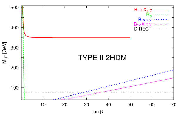
Figure 4: Direct and indirect lower bounds on $M_{H^{+}}$ from different processes in type II 2HDM as a function of $\tan\beta$. The $B\to X_{s}\gamma$ bound is the one in eq. (5.5) below.

To illustrate the incorporation of new physics in our calculation of $\bar{B}\to X_{s}\gamma$, we consider the case of the 2HDM, which also exemplifies well the importance of this decay mode for new physics. We shall update the lower bound on the charged Higgs mass in the type II model.

In the 2HDMs with vanishing tree level FCNCs, the only additional contribution with respect to the SM comes from the charged Higgs boson–top loops. It depends on the mass of the charged Higgs boson, $M_{H}$, and on the ratio of the v.e.v’s of the two Higgs doublets, $\tan\beta$. Models of type I and II differ by the way fermions couple to the Higgs doublets. In the type II model (realized in the MSSM), the charged Higgs loops always enhance BR_γ, while the decoupling occurs slowly. Therefore, this decay mode provides strong lower bounds on $M_{H}$, whose dependence on $\tan\beta$ saturates for $\tan\beta\approx 5$. Previous calculations led to $M_{H}\;\hbox to0.0pt{\lower 3.5pt\hbox{$\mathchar 0\relax\sim$}\hss}\raise 1.0pt\hbox{$>$}\;250$ GeV, independently of $\tan\beta$ [1, 37, 32]. This bound is much stronger than the one from direct searches at LEP2 ($M_{H}>78.5$ GeV [38]), and than the indirect lower limits from a number of other processes (see fig. 4) [39, 40]. In model I, $B\to X_{s}\gamma$ is less restrictive than other processes, because the charged Higgs loops tend to suppress the branching ratio and decouple for large $\tan\beta$. The most important constraint in that case comes from $R_{b}$ [1].

The LO and NLO Wilson coefficients in the 2HDM are given in eqs. (52)–(64) of the first paper in [1]. Adopting the same notation, with $y=(m_{t}(\mu_{0})/M_{H})^{2}$ and $\mu_{W}\equiv\mu_{0}$, we perform the following replacements in $K_{t}$

$$A_{0}^{t}(x) \rightarrow A_{0}^{t}(x)-2\,\delta C_{7}^{(0)\rm eff}(\mu_{0}),\hskip 42.67912ptF_{0}^{t}(x)\ \rightarrow\ F_{0}^{t}(x)-2\,\delta C_{8}^{(0)\rm eff}(\mu_{0}),$$

$$E_{0}^{t}(x) \rightarrow E_{0}^{t}(x)+E^{H}(y),$$

$$A_{1}^{t}(x) \rightarrow A_{1}^{t}(x)-2\,\left[G_{7}^{H}(y)+\Delta_{7}^{H}(y)\ln\frac{\mu_{0}^{2}}{M_{H}^{2}}\right],$$ (5.4)

$$F_{1}^{t}(x) \rightarrow F_{1}^{t}(x)-2\,\left[G_{8}^{H}(y)+\Delta_{8}^{H}(y)\ln\frac{\mu_{0}^{2}}{M_{H}^{2}}\right].$$

As mentioned above, the $\ln\mu_{0}$ terms in eq. (LABEL:Kt) should be left unchanged.

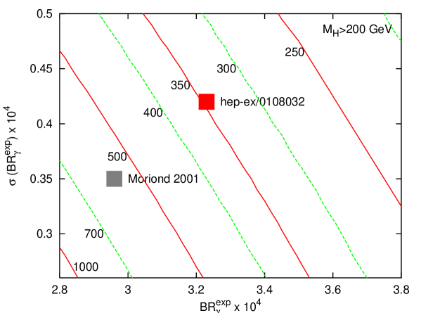
Figure 5: The 99% CL bound on the 2HDM-II charged Higgs mass from $B\to X_{s}\gamma$ as a function of the world average and of its error. The contour lines represent values which lead to the same $M_{H^{+}}$ bound. The experimental world averages evaluated with use of the preliminary [41] and published [4] CLEO results are indicated for reference.

We are now in a position to calculate the branching ratio for $B\to X_{s}\gamma$ in the 2HDM, and to find the lower bound on $M_{H}$ in model II. Since the CLEO and BELLE results (obtained with $E_{\gamma}>2.0$ GeV and 2.1 GeV, respectively, in the $\Upsilon$ frame) have been extrapolated to the “total” rate, we compare the experimental result with our prediction for $E_{\gamma}>\frac{1}{20}m_{b}$ [10]. With respect to previous analyses, the SM prediction is now higher — see eq. (4.17). Moreover, the charged Higgs contribution in model II cannot help reducing the value of BR_γ. Thus, our bound is going to be stronger than in the past [1, 37, 32]. In addition, one should take into account that for a heavy charged Higgs, the dependence of BR_γ on $M_{H}$ becomes very mild, signalling the decoupling. Consequently, a small change in BR_γ affects the $M_{H}$ bound in a significant way.

Therefore, we adopt a very conservative approach. We employ the experimental world average $(3.23\pm 0.42)\times 10^{-4}$ and scan over the main theoretical errors in our calculation — first line of eq. (4.14) — notably the one related to $m_{c}/m_{b}$ in $\langle P_{2}\rangle$. Whenever the $\mu_{b}$- and $\mu_{0}$-dependences of $BR_{\gamma}$ in the 2HDM are larger than our 4% NNLO uncertainty in eq. (4.14), we expand this error accordingly. All the remaining parametric and experimental errors are combined in quadrature. The absolute lower limit is

$$M_{H}>350~{}{\rm GeV}$$ (5.5)

for any value of $\tan\beta$. As far as the gaussian errors are concerned, this is a 99% CL bound. The 95% CL bound is 500 GeV. In view of future changes in the experimental situation, we display in fig. 5 the 99% CL bounds as functions of the central value and of the error of the world average. The dependence of the $M_{H}$ lower limit on $\tan\beta$ is shown in fig. 4.

The bound is clearly very sensitive to the way various errors are combined. For instance, if we combined all the errors in quadrature, the 99% CL absolute lower limit on $M_{H}$ would be 500 GeV. On the other hand, the way we combine the errors emphasizes the large uncertainty coming from $m_{c}(\mu)/m_{b}^{1S}$ in $\langle P_{2}\rangle$. In effect, the lower limits that we have quoted correspond to $m_{c}(m_{c})/m_{b}^{1S}=0.26$, i.e. the highest value of $m_{c}(\mu)/m_{b}^{1S}$ that is compatible with our analysis in appendix D. Had we employed $m_{c}/m_{b}=0.29\pm 0.02$ as in previous analyses and treated this error as in the derivation of eq. (5.5), the 99% (95%) CL bound would have been $M_{H}>280~{}(380)$ GeV.

In deriving the limits on $M_{H}$, we have not assumed that the 2HDM is valid for sure, i.e. we have not subtracted $\chi^{2}_{{}_{\rm best\;fit}}$ from the $\chi^{2}$ used for the test. Consequently, the statement that $M_{H}>M_{0}$ at $x\%$ CL means that the 2HDM is excluded at $x\%$ CL unless $M_{H}>M_{0}$. A different procedure consists in assuming the validity of the 2HDM and in testing $\chi^{2}-\chi^{2}_{{}_{\rm best\;fit}}$. In this case, adopting the same treatment of errors as in eq. (5.5), we obtain $M_{H}>345~{}(490)$ GeV at 99% (95%) CL.

6 Conclusions

The reanalysis of $\bar{B}\to X_{s}\gamma$ performed in the present article contains several major improvements with respect to the previous ones. In particular, the semileptonic phase–space factor is expressed in terms of an observable for which the NNLO results are known. Moreover, the RGE evolution of $m_{b}(\mu)$ in the top–quark contribution to the $b\to s\gamma$ amplitude is identified as the main reason for the huge enhancement of the branching ratio by QCD logarithms. In consequence, better control over the behaviour of QCD perturbation series is achieved. Unfortunately, the desired reduction of theoretical uncertainties significantly below the current experimental ones is found to be impossible at the NLO level, because of the strong $m_{c}$-dependence of certain two–loop diagrams with charm-quark loops.

In order to compare our final prediction (4.14) with the weighted average (1.1) of the experimental results, we have either to evaluate the theoretical errors in eq. (4.17) or rather to “take back” the extrapolation to low photon energies on the experimental side. Choosing the latter possibility, we find that the experimental result corresponding to our eq. (4.14) is

$${\rm BR}[\bar{B}\to X_{s}\gamma]^{\rm exp}_{E_{\gamma}>1.6~{}{\rm GeV}}=\frac{3.60}{3.73}(3.23\pm 0.42)\times 10^{-4}=(3.12\pm 0.41)\times 10^{-4},$$ (6.1)

where the ratio of eqs. (4.14) and (4.17) has been used as the rescaling factor. The difference between theory and experiment can now be written as

$${\rm BR}_{\gamma}^{\rm th}-{\rm BR}_{\gamma}^{\rm exp}=(3.60\pm 0.30)\times 10^{-4}-(3.12\pm 0.41)\times 10^{-4}=(0.48\pm 0.50)\times 10^{-4},$$ (6.2)

which is compatible with zero. Based on the present experimental information, we have shown that the Two–Higgs–Doublet–Model II with a charged Higgs boson lighter than 350 GeV is strongly disfavoured.

Appendix A

In this appendix, our numerical input parameters are collected. From ref. [29], we take $M_{Z}=91.1882$ GeV, $M_{W}=80.419$ GeV, $\alpha_{em}=1/137.036$, $\alpha_{s}(M_{Z})=0.1185\pm 0.0020$, $m_{c}^{\overline{\rm MS}}(m_{c}^{\overline{\rm MS}})=(1.25\pm 0.10)$ GeV and BR$[\bar{B}\to X_{c}e\bar{\nu}]_{\rm exp}=0.1045\pm 0.0021$.

For the $b$-quark mass in the so-called 1S-scheme, we use $m_{b}^{1S}=(4.69\pm 0.03)$ GeV [42]. As far as the top-quark mass is concerned, $m_{t}^{\overline{\rm MS}}(m_{t}^{\overline{\rm MS}})=(165\pm 5)$ GeV is used, which corresponds to $m_{t}^{\rm pole}=174.3\pm 5.1$ GeV [29].

In several places, definitions of $m_{t}$ and $m_{b}$ have been left unspecified, because it would become relevant only at higher orders of perturbation theory. In such places, $m_{t}^{\overline{\rm MS}}(m_{t}^{\overline{\rm MS}})$ and $m_{b}^{1S}$ are used.

When the $\mu$-dependence is being tested, each scale is made to vary from half to twice its central value. The central value of $\mu_{b}$ is chosen to be $m_{b}$. For the matching scale $\mu_{0}$, we take the central value of $M_{W}$ in $K_{c}$ and in the quantities for which no flavour splitting is performed. In $K_{t}$ and in the mass ratio $r(\mu_{0})$, the central value of $\mu_{0}$ is set to $m_{t}$.

The final result (4.14) for the branching ratio (3.1) has been found by using the above inputs as well as the quantities specified in eqs.  (4.5), (4.6), (4.7), (B.4), (C.13) and (D.9).

Appendix B

Here, we determine the mass ratio $r(\mu_{0})=m_{b}(\mu_{0})^{\overline{\rm MS}}/m_{b}^{1S}$. The NLO result reads

$$r_{\scriptscriptstyle NLO}(\mu_{0})=\left(\frac{\alpha_{s}(\mu_{0})}{\alpha_{s}(m_{b})}\right)^{\frac{12}{23}}\left\{1+\frac{\alpha_{s}(m_{b})}{4\pi}\left[\frac{7462}{1587}\;\frac{\alpha_{s}(\mu_{0})}{\alpha_{s}(m_{b})}-\frac{15926}{1587}\right]+\frac{2}{9}\alpha_{s}(m_{b})^{2}\right\}~{}\mathrel{\mathop{\kern 0.0pt=}\limits_{\mu_{0}=m_{t}}}~{}0.611.$$

(B.1)

The ${\cal O}(\alpha_{s}^{2})$ term is included along the lines of the $\Upsilon$ expansion [21]. Its effect on $r$ is at the level of 1% only, and it is offset by an analogous term in $K_{t}$ (LABEL:Kt).

Since $m_{b}(\mu_{0})$ could, in principle, be determined from a high-energy observable (e.g. the Higgs width), we are allowed to calculate the ratio $r(\mu_{0})$ using as many orders of perturbation theory as are currently known, i.e. up to ${\cal O}(\epsilon^{3})$ in the $\Upsilon$ expansion.

From eq. (168) of ref. [42], we find

$$\frac{m_{b}^{\overline{\rm MS}}(m_{b}^{\overline{\rm MS}})}{m_{b}^{1S}}\approx 0.889\left(\frac{\alpha_{s}(M_{Z})}{0.1185}\right)^{-0.26}\left(\frac{m_{b}^{1S}}{4.69}\right)^{0.04}\left(\frac{m_{c}(m_{c})}{1.25}\right)^{-0.003}\left(\frac{\mu_{b}}{4.69}\right)_{\cdot}^{0.006}$$ (B.2)

All the masses and renormalization scales in eqs. (B.2)–(B.4) are expressed in GeV. The dependence on $\mu_{b}$ in eq. (B.2) originates only from the fact that $\alpha_{s}(\mu_{b})$ rather than $\alpha_{s}(m_{b})$ has been used in evaluating this relation. Varying $\mu_{b}$ by a factor of 2 around 4.69 GeV gives us an estimate of $\pm 0.4\%$ for the neglected higher-order effects.

The four–loop RGE for the quark mass imply

$$\frac{m_{b}^{\overline{\rm MS}}(m_{t})}{m_{b}^{\overline{\rm MS}}(m_{b}^{\overline{\rm MS}})}\approx 0.650\left(\frac{\alpha_{s}(M_{Z})}{0.1185}\right)^{-0.72}\left(\frac{m_{b}^{\overline{\rm MS}}(m_{b}^{\overline{\rm MS}})}{4.17}\right)^{0.19}\left(\frac{m_{t}}{165}\right)_{,}^{-0.08}$$ (B.3)

where the higher-order uncertainty is negligible (below 0.2%). Combining eqs. (B.2) and (B.3), we find

$$r(m_{t})\equiv\frac{m_{b}^{\overline{\rm MS}}(m_{t})}{m_{b}^{1S}}\approx 0.578\left(\frac{\alpha_{s}(M_{Z})}{0.1185}\right)^{-1.0}\left(\frac{m_{b}^{1S}}{4.69}\right)^{0.23}\left(\frac{m_{c}(m_{c})}{1.25}\right)^{-0.003}\left(\frac{m_{t}}{165}\right)^{-0.08}\left(\frac{\mu_{b}}{4.69}\right)_{\cdot}^{0.006}~{}~{}$$ (B.4)

The above approximate formula works with better than 0.2% accuracy (compared with the complete one ) when the input parameters vary within their errors (see appendix A).

It is important to note that the central value in eq. (B.4) is 5.4% less than $r_{\scriptscriptstyle NLO}$ in eq. (Appendix B). The main reason of this suppression is the $-3.2\%$ higher-than-NLO correction to $m_{b}^{\overline{\rm MS}}(m_{b}^{\overline{\rm MS}})/m_{b}^{1S}$ (see eq. (99) of ref. [42]). Switching from two-loop to four-loop RGE causes a reduction of $r$ by only $0.7\%$. Additional effects originate from the fact that the scales $\mu=m_{b}^{1S}$ and $\mu=m_{b}(m_{b})$ have been identified in eq. (Appendix B).

The ratio $r(\mu_{0})$ depends only logarithmically on the actual value of $m_{b}^{1S}$. This is reflected in eq. (B.4) where the power of $m_{b}^{1S}/4.69$ is equal to 0.23 only. Consequently, our results are not very sensitive to the numerical input we use for $m_{b}^{1S}$. They would not change much if instead of $m_{b}^{1S}$ we used another definition of the ”kinetic” mass of the b-quark, e.g. the ones defined in refs. [43, 44], or the $\overline{\rm MS}$ mass at appropriately chosen $\mu$. However, in such a case, eq. (LABEL:Kt) would need to be modified accordingly.

Appendix C

The present appendix is devoted to a determination of the semileptonic phase-space factor:

$$C=\left|\frac{V_{ub}}{V_{cb}}\right|^{2}\frac{\Gamma[\bar{B}\to X_{c}e\bar{\nu}]}{\Gamma[\bar{B}\to X_{u}e\bar{\nu}]}$$ (C.1)

along the lines of the $\Upsilon$ expansion [21].

We begin with the NNLO expressions for both decay rates expressed in terms of pole quark masses and $\alpha_{s}\equiv\alpha_{s}^{(n_{f}=5)}(m_{b})\approx 0.219$:

$$\Gamma[\bar{B}\to X_{c}e\bar{\nu}] = \frac{G_{F}^{2}(m_{b}^{\rm pole})^{5}}{192\pi^{3}}|V_{cb}|^{2}g(z_{p})\left[1+\epsilon\frac{\alpha_{s}}{\pi}p_{c}^{(1)}(z_{p})+\epsilon^{2}\frac{\alpha_{s}^{2}}{\pi^{2}}p_{c}^{(2)}(z_{p})\right.$$ (C.2)

$$\hskip 125.19212pt\left.+\frac{\lambda_{1}}{2m_{b}^{2}}+\frac{\lambda_{2}}{m_{b}^{2}}\left(\frac{3}{2}-\frac{6(1-z_{p})^{4}}{g(z_{p})}\right)\right],$$

$$\Gamma[\bar{B}\to X_{u}e\bar{\nu}] = \frac{G_{F}^{2}(m_{b}^{\rm pole})^{5}}{192\pi^{3}}|V_{ub}|^{2}\left[1+\epsilon\frac{\alpha_{s}}{\pi}p_{u}^{(1)}+\epsilon^{2}\frac{\alpha_{s}^{2}}{\pi^{2}}p_{u}^{(2)}(z_{p})+\frac{\lambda_{1}}{2m_{b}^{2}}-\frac{9\lambda_{2}}{2m_{b}^{2}}\right],$$ (C.3)

where $z_{p}=(m_{c}^{\rm pole}/m_{b}^{\rm pole})^{2}$ and $g(z)=1-8z+8z^{3}-z^{4}-12z^{2}\ln z$. The auxiliary parameter $\epsilon\equiv 1$ will be helpful below in denoting orders of the $\Upsilon$ expansion.

The perturbative corrections are as follows [45]:

$$p_{c}^{(1)}(z) = -\frac{2h(z)}{3g(z)},$$ (C.4)

$$p_{c}^{(2)}(z=0.09) = -1.68\beta_{0}^{(4)}+(1.4\pm 0.4)=-12.6\pm 0.4,$$ (C.5)

$$p_{u}^{(1)} = \frac{25}{6}-\frac{2}{3}\pi^{2},$$ (C.6)

$$p_{u}^{(2)}(z) = -3.22\beta_{0}^{(4)}+5.53+f_{u}(z)=-21.30+f_{u}(z),$$ (C.7)

where $\beta_{0}^{(n_{f})}=11-\frac{2}{3}n_{f}$  and

$$h(z) = -(1-z^{2})\left(\frac{25}{4}-\frac{239}{3}z+\frac{25}{4}z^{2}\right)+z\ln z\left(20+90z-\frac{4}{3}z^{2}+\frac{17}{3}z^{3}\right)+z^{2}\ln^{2}z\;(36+z^{2})$$

$$+(1-z^{2})\left(\frac{17}{3}-\frac{64}{3}z+\frac{17}{3}z^{2}\right)\ln(1-z)-4(1+30z^{2}+z^{4})\ln z\;\ln(1-z)$$

$$-(1+16z^{2}+z^{4})[6{\rm Li}_{2}(z)-\pi^{2}]-32z^{3/2}(1+z)\left[\pi^{2}-4{\rm Li}_{2}(\sqrt{z})+4{\rm Li}_{2}(-\sqrt{z})-2\ln\left(\frac{1-\sqrt{z}}{1+\sqrt{z}}\right)\ln z\right].$$

As far as the charm-mass correction $f_{u}(z)$ in eq. (C.7) is concerned, the only thing we know for sure is that $f_{u}(0)=0$. A rough estimate of $f_{u}(0.09)$ can be obtained by considering the relation between pole and $\overline{\rm MS}$ bottom masses, for which charm-loop corrections are known at two [46] and three [42] loops. Similarly to $f_{u}(z)$, they originate from charm loop insertions on gluon lines. For $m_{c}/m_{b}=0.3$, we learn from ref. [42] that two-loop charm mass effects lead to an extra term $0.43(\alpha_{s}/\pi)^{2}$. As the charm loops are closely related to the BLM corrections, which amount to $1.56\beta_{0}(\alpha_{s}/\pi)^{2}$ in the relation between masses, we can rescale them by a factor $-3.22/1.56$ to obtain $f_{u}(0.09)\sim-0.9$. Of course, this is only a very rough estimate, and an actual calculation of $f_{u}(z)$ would be welcome.

When the ratio (C.1) is calculated, the overall factors of $(m_{b}^{\rm pole})^{5}$ cancel. The remaining explicit dependence on pole quark masses can be eliminated with the help of the following relation:

$$\frac{m_{c}^{\rm pole}}{m_{b}^{\rm pole}}=1-\frac{m_{b}^{\rm pole}-m_{c}^{\rm pole}}{m_{b}^{\rm pole}}=1-\frac{\overline{m}_{B}-\overline{m}_{D}+\frac{\lambda_{1}}{2\overline{m}_{B}}-\frac{\lambda_{1}}{2\overline{m}_{D}}+{\cal O}\left(\frac{\Lambda_{\rm QCD}^{3}}{\overline{m}_{D}^{2}}\right)}{\frac{1}{2}m_{\Upsilon}\left(1-\frac{\Delta^{2}}{(m_{\Upsilon}/2)^{2}}\right)\left\{1+\epsilon\frac{(\alpha_{s}C_{F})^{2}}{8}\left[1+\epsilon\frac{\alpha_{s}}{\pi}Y+{\cal O}(\alpha_{s}^{2})\right]\right\}},\hskip 11.38109pt$$ (C.8)

with $C_{F}=\frac{4}{3}$, $m_{\Upsilon}\approx 9.460$ GeV, $\overline{m}_{B}=\frac{1}{8}(3m_{B^{\star\pm}}+m_{B^{\pm}}+3m_{B^{\star 0}}+m_{B^{0}})\approx 5.314$ GeV and $\overline{m}_{D}=\frac{1}{8}(3m_{D^{\star\pm}}+m_{D^{\pm}}+3m_{D^{\star 0}}+m_{D^{0}})\approx 1.973$ GeV. In the denominator, $\Delta$ describes the non-perturbative contribution responsible for the difference between $\frac{1}{2}m_{\Upsilon}$ and $m_{b}^{1S}$. From ref. [42], one finds

$$\frac{\Delta^{2}}{(m_{\Upsilon}/2)} = (0.04\pm 0.03)~{}{\rm GeV},$$ (C.9)

$$Y = \frac{203}{18}-\frac{25}{3}\ln(\alpha_{s}C_{F})+y\left(\frac{3m_{c}}{\alpha_{s}m_{\Upsilon}}\right)$$ (C.10)

with

$$y(a)=\frac{2}{3}\ln\frac{a}{2}+\frac{\pi}{2}a-\frac{4}{3}a^{2}+\frac{2\pi}{3}a^{3}+\frac{4-2a^{2}-8a^{4}}{3\sqrt{a^{2}-1}}\arctan\frac{\sqrt{a-1}}{\sqrt{a+1}}.$$ (C.11)

Below, $m_{c}(m_{c})\approx 1.25$ GeV [29] will be used in this function. The influence of $y(a)$ on $C$ is less than 0.3%, so it does not matter what definition of $m_{c}$ is chosen here.

In the following, we shall make use of eq. (C.8), and expand all the functions of $z_{p}$ in eqs. (C.2) and (C.3) around

$$z_{0}=\left(1-\frac{\overline{m}_{B}-\overline{m}_{D}}{m_{\Upsilon}/2}\right)^{2}\approx 0.0863,$$ (C.12)

neglecting ${\cal O}(\epsilon^{3})$, ${\cal O}(\alpha_{s}^{4})$, ${\cal O}(\Lambda_{\scriptscriptstyle QCD}^{3}/m_{Q}^{3})$ and ${\cal O}(\epsilon\times\Lambda_{\scriptscriptstyle QCD}^{2}/m_{Q}^{2})$. As argued in ref. [21], the leading renormalons cancel when such an expansion is performed for physical observables. Indeed, the QCD perturbation series converges remarkably well in our final result for the ratio (C.1):

$$C = g(z_{0})\left\{1+\epsilon\left[\frac{\alpha_{s}}{\pi}\left(p_{c}^{(1)}(z_{0})-p_{u}^{(1)}\right)+\kappa\frac{(\alpha_{s}C_{F})^{2}}{8}\right]\right.$$ (C.13)

$$+ \left.\epsilon^{2}\left[\frac{\alpha_{s}^{2}}{\pi^{2}}\left(p_{c}^{(2)}(z_{0})-p_{u}^{(2)}(z_{0})+p_{u}^{(1)}(z_{0})^{2}-p_{c}^{(1)}(z_{0})p_{u}^{(1)}\right)+\kappa\frac{(\alpha_{s}C_{F})^{2}\alpha_{s}}{8\pi}\left(Y-p_{u}^{(1)}-\frac{2h^{\prime}(z_{0})}{3g^{\prime}(z_{0})}\right)\right]\right.$$

$$\left.\hskip 42.67912pt+\frac{\kappa\lambda_{1}}{2\overline{m}_{B}\overline{m}_{D}}+\frac{24\lambda_{2}}{m_{\Upsilon}^{2}}\left(1-\frac{(1-z_{0})^{4}}{g(z_{0})}\right)-\frac{\kappa\Delta^{2}}{(m_{\Upsilon}/2)^{2}}\right\}$$

$$\approx 0.534\left[1+0.019\epsilon+(0.001-0.005f_{u}(z_{0})\pm 0.002)\epsilon^{2}-\frac{\lambda_{1}}{7.1~{}{\rm GeV}^{2}}-\frac{\lambda_{2}}{12~{}{\rm GeV}^{2}}+\frac{\Delta^{2}}{7.6~{}{\rm GeV}^{2}}\right]$$

$$= 0.575\times(1\pm 0.01_{\rm pert}\pm 0.02_{\lambda_{1}}\pm 0.02_{\Delta}),$$

where

$$\kappa=2\sqrt{z_{0}}\left(1-\sqrt{z_{0}}\,\right)\frac{g^{\prime}(z_{0})}{g(z_{0})}\approx 2.94.$$ (C.14)

In the middle step, the error in the ${\cal O}(\epsilon^{2})$ term originates only from $p_{u}^{(2)}(z_{0})=-12.6\pm 0.4$ (see eq. (C.5)). In the last step, $f_{u}(z_{0})$ is set to $-0.9$, and an overall $\pm 1\%$ perturbative uncertainty is assumed, resulting from the fact that our estimate of $f_{u}(z_{0})$ is very rough, from the error in $p_{u}^{(2)}(z_{0})$ and from missing perturbative higher orders. As far as the non-perturbative parameters are concerned, we use $\lambda_{1}=(-0.27\pm 0.10\pm 0.04)~{}{\rm GeV}^{2}$ [21], $\lambda_{2}=0.12~{}{\rm GeV}^{2}$ and eq. (C.9).

A delicate point in our calculation of $C$ is the fact that the unknown ${\cal O}(\Lambda_{\scriptscriptstyle QCD}^{3}/\overline{m}_{D}^{2})$ corrections have been neglected in the numerator of eq. (C.8). Their potential effect can be studied by replacing $\lambda_{1}\to\lambda_{1}\pm{\cal O}(\Lambda_{\scriptscriptstyle QCD}^{3})/\overline{m}_{D}$ in eq. (C.13). However, if such corrections were sizeable, they would affect the determination of $\lambda_{1}$ from the semileptonic spectrum in ref. [21]. In the present paper, we assume that those corrections are included in the error of $\lambda_{1}$ (and in its central value). A further study of this point is warranted.

It is worth mentioning that our final central value $C=0.575$ can be reproduced from the ratio of eqs. (C.2) and (C.3) expanded in $\alpha_{s}$ and $\lambda_{i}$, for $z_{p}=0.285^{2}$ at NLO, and $z_{p}=0.298^{2}$ at NNLO. Those two values are consistent with $z_{p}=(0.29\pm 0.02)^{2}$ which has been used in many previous analyses of $\bar{B}\to X_{s}\gamma$. On the other hand, when $z_{p}=(0.29\pm 0.02)^{2}$ is used in such a ratio, one obtains at NNLO

$$C_{\rm direct}=0.595\times(1\pm 0.08\pm 0.05),$$ (C.15)

where the first error comes from $z_{p}$, and the second one from poor convergence of the perturbation series. The uncertainties here are much larger than in the result (C.13) obtained with the help of the $\Upsilon$ expansion.

Appendix D

In this appendix, we present the analytical formulae and calculate the numerical values of the functions $a(z)$ and $b(z)$ that occur in the expression for $K_{c}$ (3.7). Those two functions of $z=(m_{c}/m_{b})^{2}$ originate from the two–loop $b\to s\gamma$ matrix elements of the 4-quark operators $P_{1}$ and $P_{2}$ (2.1). The relevant diagrams are shown in fig. 6. They were calculated in ref. [11]. Their colour structure implies that $\langle P_{1}\rangle=-\frac{1}{6}\langle P_{2}\rangle$. Additive constants in the functions $a(z)$ and $b(z)$ are chosen in such a way that both functions vanish at $z=0$. Explicitly,

(D.1)

$$\begin{array}[]{rcl}a(z)&=&\frac{16}{9}\left\{\left[\frac{5}{2}-\frac{1}{3}\pi^{2}-3\zeta(3)+\left(\frac{5}{2}-\frac{3}{4}\pi^{2}\right)L+\frac{1}{4}L^{2}+\frac{1}{12}L^{3}\right]z\right.\\[5.69054pt] &&\hskip 8.53581pt\left.+\left[\frac{7}{4}+\frac{2}{3}\pi^{2}-\frac{1}{2}\pi^{2}L-\frac{1}{4}L^{2}+\frac{1}{12}L^{3}\right]z^{2}+\left[-\frac{7}{6}-\frac{1}{4}\pi^{2}+2L-\frac{3}{4}L^{2}\right]z^{3}\right.\\[5.69054pt] &&\hskip 8.53581pt\left.+i\pi\left[\left(2-\frac{1}{6}\pi^{2}+\frac{1}{2}L+\frac{1}{2}L^{2}\right)z+\left(\frac{1}{2}-\frac{1}{6}\pi^{2}-L+\frac{1}{2}L^{2}\right)z^{2}+z^{3}\right]\right\}+{\cal O}(z^{4}L^{4}),\\[8.53581pt] b(z)&=&-\frac{8}{9}\left\{\left(-3+\frac{1}{6}\pi^{2}-L\right)z+\left(\frac{1}{2}+\pi^{2}-2L-\frac{1}{2}L^{2}\right)z^{2}+\left(-\frac{25}{12}-\frac{1}{9}\pi^{2}-\frac{19}{18}L+2L^{2}\right)z^{3}\right.\\[5.69054pt] &&\hskip 8.53581pt\left.-\frac{2}{3}\pi^{2}z^{3/2}+i\pi\left[-z+(1-2L)z^{2}+\left(-\frac{10}{9}+\frac{4}{3}L\right)z^{3}\right]\right\}+{\cal O}(z^{4}L^{4}),\end{array}$$ (D.7)

where $L=\ln z$.

The imaginary parts of $a(z)$ and $b(z)$ have very little influence on our prediction for BR_γ. Since the LO amplitude is real, they affect the r.h.s. of eq. (3.5) only via ${\cal O}(\alpha_{s}^{2})$ terms that we neglect anyway and via the very small ${\cal O}(V_{ub})$ correction in eq. (3.7). If we included the imaginary parts of $K_{c}$ and $K_{t}$, our final result (4.14) would get enhanced by only around 0.5%.

Figure 6: Leading contributions to the $b\to s\gamma$ matrix elements of $P_{1}$ and $P_{2}$.

$b$                   $s$    $b$                  $s$
                     $c$            $c$                          $c$            $c$
                                                                                                 $c$           $c$
             $b$              $s$     $b$             $s$    $b$            $s$     $b$              $s$

As we have mentioned in the introduction, the choice of renormalization scheme for $m_{c}$ and $m_{b}$ in $\langle P_{1,2}\rangle$ is very important for BR_γ. In principle, this choice is a NNLO issue that can be resolved only after calculating three-loop corrections to the diagrams of fig. 6. Since calculating finite parts of such diagrams would be a very difficult task at present, we have to guess what the optimal choice of $m_{c}$ and $m_{b}$ is, on the basis of our experience from other calculations.

All the factors of $m_{c}$ in $\langle P_{1,2}\rangle$ originate from explicit mass factors in the charm-quark propagators. In the real parts of $\langle P_{1,2}\rangle$, those charm quarks are dominantly off-shell, with momentum scale $\mu$ set by $m_{b}$. Actually, we are not able to decide whether this scale is $m_{b}$, $\frac{1}{2}m_{b}$ or $\frac{1}{3}m_{b}$. Therefore, we shall vary $\mu$ between $m_{c}\sim\frac{1}{3}m_{b}$ and $m_{b}$, and use $m_{c}^{\overline{\rm MS}}(\mu)$ in $a(z)$ and $b(z)$.

As far as the factors of $m_{b}$ are concerned, they originate either from the overall momentum release in $b\to s\gamma$ or from the explicit appearance of $m_{b}$ in the $b$-quark propagators. In the first case, the appropriate choice of $m_{b}$ is a low-virtuality mass. In the second case, there is no intuitive argument that could tell us whether $m_{b}^{\rm pole}$ or $m_{b}(m_{b})$ is preferred. However, we think that as long as the three-loop diagrams remain unknown, the best choice is to set all the factors of $m_{b}$ equal to $m_{b}^{1S}$ in $a(z)$ and $b(z)$. The distinction between $m_{b}^{1S}$ and $m_{b}^{\rm pole}$ as well as the infrared sensitivity of the pole mass can be ignored here, because the uncertainties due to $m_{c}(\mu)$ are very large.

In determining the optimal renormalization scheme for $m_{b}$ in the ratio $m_{c}^{2}/m_{b}^{2}$, we have to take into account that the considered perturbative amplitude arises as a particular term in the operator product expansion for the inclusive decay of the $\bar{B}$ meson. Thus, the ratio $m_{c}^{2}/m_{b}^{2}$ should be understood as $m_{c}^{2}/Q^{2}$, where $Q^{2}$ is the squared ”mean” momentum of the $b$-quark inside the $\bar{B}$-meson. Its value is given by one of the ”kinetic” b-quark masses [21, 43, 44], e.g. $(m_{b}^{1S})^{2}$. Given the large error in $m_{c}(\mu)$, it does not matter which definition of the bottom kinetic mass is chosen here.

It remains to determine the numerical value of $m_{c}^{\overline{\rm MS}}(\mu)/m_{b}^{1S}$. From $m_{c}=m_{c}(m_{c})=(1.25\pm 0.10)$ GeV [29] and the RGE for $m_{c}(\mu)$, we find

$$m_{c}^{\overline{\rm MS}}(\mu)/m_{b}^{\rm 1S}=0.22\pm 0.04,$$ (D.9)

which implies

$$a(z) = (0.97\pm 0.25)\;+\;i(1.01\pm 0.15),$$ (D.10)

$$b(z) = (-0.04\pm 0.01)\;+\;i(0.09\pm 0.02),$$ (D.11)

for $\mu$ varying between $m_{c}$ and $m_{b}$. The uncertainty in $m_{c}(m_{c})$ is practically irrelevant here, when compared to the dominant error that originates from a variation of $\mu$. We also note that our central value $m_{c}/m_{b}=0.22$, is very close to the RG-invariant $\overline{\rm MS}$ ratio $m_{c}(\mu)/m_{b}(\mu)=0.215$.

Appendix E

Here, we discuss the function $B(E_{0})$ in eq. (3.5) that arises from $b\to s\gamma g$ and $b\to s\gamma q\bar{q}$ with $q=u,d,s$:

$$B(E_{0})=\frac{\alpha_{s}(\mu_{b})}{\pi}\sum_{\begin{array}[]{c}\\[-19.91692pt] {\scriptscriptstyle i,j=1,...,8}\\[-5.69054pt] {\scriptscriptstyle i\leq j}\end{array}}C_{i}^{(0)\rm eff}(\mu_{b})\;\;C_{j}^{(0)\rm eff}(\mu_{b})\;\;\phi_{ij}\left(1-\frac{2E_{0}}{m_{b}}\right)\;+\;\beta_{q\bar{q}}(E_{0}).$$ (E.1)

The functions $\phi_{ij}(\delta)$ originate from the gluon bremsstrahlung $b\to s\gamma g$ [13, 14, 47]. For $i,j\in\{1,2,7,8\}$ their explicit form is as follows:

$$\phi_{22}(\delta) = \frac{16z}{27}\left[\delta\int_{0}^{(1-\delta)/z}dt\;(1-zt)\left|\frac{G(t)}{t}+\frac{1}{2}\right|^{2}\;+\;\int_{(1-\delta)/z}^{1/z}dt\;(1-zt)^{2}\left|\frac{G(t)}{t}+\frac{1}{2}\right|^{2}\right],$$ (E.2)

$$\phi_{27}(\delta) = -\frac{8z^{2}}{9}\left[\delta\int_{0}^{(1-\delta)/z}dt\;{\rm Re}\left(G(t)+\frac{t}{2}\right)\;+\;\int_{(1-\delta)/z}^{1/z}dt\;(1-zt){\rm Re}\left(G(t)+\frac{t}{2}\right)\right],$$ (E.3)

$$\phi_{77}(\delta) = -\frac{2}{3}\ln^{2}\delta-\frac{7}{3}\ln\delta-\frac{31}{9}+\frac{10}{3}\delta+\frac{1}{3}\delta^{2}-\frac{2}{9}\delta^{3}+\frac{1}{3}\delta(\delta-4)\ln\delta,$$ (E.4)

$$\phi_{78}(\delta) = \frac{8}{9}\left[{\rm Li}_{2}(1-\delta)-\frac{\pi^{2}}{6}-\delta\ln\delta+\frac{9}{4}\delta-\frac{1}{4}\delta^{2}+\frac{1}{12}\delta^{3}\right],$$ (E.5)

$$\phi_{88}(\delta) = \frac{1}{27}\left\{-2\ln\frac{m_{b}}{m_{s}}\left[\delta^{2}+2\delta+4\ln(1-\delta)\right]\right.$$ (E.6)

$$\hskip 28.45274pt\left.+4{\rm Li}_{2}(1-\delta)-\frac{2\pi^{2}}{3}-\delta(2+\delta)\ln\delta+8\ln(1-\delta)-\frac{2}{3}\delta^{3}+3\delta^{2}+7\delta\right\},$$

$$\phi_{11}=\frac{1}{36}\phi_{22},~{}~{}~{}~{}~{}~{}\phi_{12}=-\frac{1}{3}\phi_{22},~{}~{}~{}~{}~{}~{}\phi_{17}=-\frac{1}{6}\phi_{27},~{}~{}~{}~{}~{}~{}\phi_{18}=\frac{1}{18}\phi_{27},~{}~{}~{}~{}~{}~{}\phi_{28}=-\frac{1}{3}\phi_{27}.$$ (E.7)

They are identical to the $f_{ij}(\delta)$ used in many previous analyses of $\bar{B}\to X_{s}\gamma$, except for the case $i=j=7$. The difference between $\phi_{77}(\delta)$ and $f_{77}(\delta)$ from eq. (37) of ref. [12] is given by the first three terms in eq. (E.4): the Sudakov logarithms ($\ln^{2}\delta$, $\ln\delta$) and a constant term that makes $\phi_{77}(\delta)$ vanish at $\delta\to 1$. For simplicity, we refrain from resumming the Sudakov logarithms here, because we are interested only in energy cut–offs $E_{0}<2.1$ GeV ($\delta>0.1$), for which $|\phi_{77}(\delta)|<1$, i.e. the logarithmic divergence of $\phi_{77}(\delta)$ at $\delta\to 0$ is not yet relevant.

The function $G(t)$ that appears in eqs. (E.2) and (E.3) reads

$$G(t)=\left\{\begin{array}[]{cc}-2\arctan^{2}\sqrt{t/(4-t)},&\mbox{ for $t<4$}\vspace{0.2cm}\\ -\pi^{2}/2+2\ln^{2}[(\sqrt{t}+\sqrt{t-4})/2]-2i\pi\ln[(\sqrt{t}+\sqrt{t-4})/2],&\mbox{ for $t\geq 4$}.\end{array}\right.$$ (E.8)

In our numerical analysis, the parameter $z=m_{c}^{2}/m_{b}^{2}$ entering those equations is set equal to $(0.22\pm 0.04)^{2}$, as determined in appendix D. In eq. (E.6), we follow ref. [12] and use $m_{b}/m_{s}=50$.

The functions $\phi_{ij}$ with $3\leq(i~{}{\rm or}~{}j)\leq 6$ have only a 0.1% effect on BR$[\bar{B}\to X_{s}\gamma]_{E_{\gamma}>1.6\;{\rm GeV}}$. Therefore, we shall not give them explicitly here. They can be read from the results of ref. [14].

The coefficients $C_{i}^{(0)\rm eff}(\mu_{b})$ are equal to those in eqs. (20) and (22) of ref. [12]. They read ($C_{i}=C_{i}^{\rm eff}$ for $i=1,...,6$)

$$\begin{array}[]{rcrll}C^{(0)}_{1}(\mu_{b})&=&\eta^{a_{3}}&-\eta^{a_{4}},&\\[5.69054pt] C^{(0)}_{2}(\mu_{b})&=&\frac{2}{3}\eta^{a_{3}}&+\frac{1}{3}\eta^{a_{4}},&\\[5.69054pt] C^{(0)}_{3}(\mu_{b})&=&\frac{2}{63}\eta^{a_{3}}&-\frac{1}{27}\eta^{a_{4}}&-0.0659\,\eta^{a_{5}}+0.0595\,\eta^{a_{6}}-0.0218\,\eta^{a_{7}}+0.0335\,\eta^{a_{6}},\\[5.69054pt] C^{(0)}_{4}(\mu_{b})&=&\frac{1}{21}\eta^{a_{3}}&+\frac{1}{9}\eta^{a_{4}}&+0.0237\,\eta^{a_{5}}-0.0173\,\eta^{a_{6}}-0.1336\,\eta^{a_{7}}-0.0316\,\eta^{a_{8}},\\[5.69054pt] C^{(0)}_{5}(\mu_{b})&=&-\frac{1}{126}\eta^{a_{3}}&+\frac{1}{108}\eta^{a_{4}}&+0.0094\,\eta^{a_{5}}-0.0100\,\eta^{a_{6}}+0.0010\,\eta^{a_{7}}-0.0017\,\eta^{a_{8}},\\[5.69054pt] C^{(0)}_{6}(\mu_{b})&=&-\frac{1}{84}\eta^{a_{3}}&-\frac{1}{36}\eta^{a_{4}}&+0.0108\,\eta^{a_{5}}+0.0163\,\eta^{a_{6}}+0.0103\,\eta^{a_{7}}+0.0023\,\eta^{a_{8}},\\[5.69054pt] C^{(0)\rm eff}_{7}(\mu_{b})&=&\lx@intercol\left(-\frac{4}{3}F_{0}^{t}(x)+\frac{42678}{30253}\right)\eta^{a_{1}}+\left(-\frac{1}{2}A^{t}_{0}(x)+\frac{4}{3}F_{0}^{t}(x)-\frac{86697}{103460}\right)\eta^{a_{2}}\hfil\lx@intercol\\[8.53581pt] &&-\frac{3}{7}\eta^{a_{3}}&-\frac{1}{14}\eta^{a_{4}}&-0.6494\,\eta^{a_{5}}-0.0380\,\eta^{a_{6}}-0.0185\,\eta^{a_{7}}-0.0057\,\eta^{a_{8}},\\[5.69054pt] C^{(0)\rm eff}_{8}(\mu_{b})&=&\lx@intercol\left(-\frac{1}{2}F_{0}^{t}(x)+\frac{64017}{121012}\right)\eta^{a_{1}}\hfil\lx@intercol&-0.9135\,\eta^{a_{5}}+0.0873\,\eta^{a_{6}}-0.0571\,\eta^{a_{7}}+0.0209\,\eta^{a_{8}},\end{array}$$ (E.18)

where $x=m_{t}(m_{t})^{2}/M_{W}^{2}$. The powers $a_{i}$ can be found in table 1, in section 3.

It is important to mention that the sensitivity of $B(E_{0})$ to $m_{b}$ via the argument of $\phi_{ij}$ is rather weak when $E_{0}=1.6$ GeV. When $m_{b}$ is varied between 4.5 and 4.9 GeV here, our final result for BR$[\bar{B}\to X_{s}\gamma]_{E_{\gamma}>1.6\,{\rm GeV}}$ is affected by only around 0.7%. In section 4, we have neglected this uncertainty, and used $m_{b}=m_{b}^{1S}$ in eq. (E.1).

The term denoted by $\beta_{q\bar{q}}(E_{0})$ in eq. (E.1) stands for the contributions from $b\to sq\bar{q}\gamma$ transitions with $q=u,d,s$. Perturbatively, such effects on $\Gamma[b\to X_{s}\gamma]$ are suppressed by either

$$\left|\frac{C^{(0)}_{3,...,6}(\mu_{b})}{C^{(0)\rm eff}_{7}(\mu_{b})}\right|^{2}<0.05\hskip 56.9055pt{\rm or}\hskip 56.9055pt\left|\frac{V^{*}_{us}V_{ub}}{V_{ts}^{*}V_{tb}}\frac{C_{2}^{(0)}(\mu_{b})}{C^{(0)\rm eff}_{7}(\mu_{b})}\right|^{2}\approx 0.002$$ (E.20)

with respect to the leading terms. Further suppression occurs when we restrict ourselves to high-energy photons [47]. In our numerical analysis we have set $\beta_{q\bar{q}}(E_{0})$ to zero without including any additional uncertainty, which we expect to be acceptable at present for an energy cut–off $E_{0}\geq 1.6$ GeV.

References

• [1] M. Ciuchini, G. Degrassi, P. Gambino and G.F. Giudice, Nucl. Phys. B527 (1998) 21,
ibid. B534 (1998) 3.
• [2] G. Degrassi, P. Gambino and G.F. Giudice, JHEP 0012 (2000) 009.
• [3] M. Misiak, S. Pokorski and J. Rosiek, hep-ph/9703442, published in the Review Volume “Heavy Flavors II”, eds. A.J. Buras and M. Lindner, World Scientific Publishing Co., Singapore, 1998.
• [4] S. Chen et al. (CLEO Collaboration), hep-ex/0108032.
• [5] H. Tajima, talk given at the 20th International Symposium on Lepton-Photon Interactions, Rome, July 2001.
• [6] R. Barate et al., Phys. Lett. B429 (1998) 169.
• [7] M.B. Voloshin, Phys. Lett. B397 (1997) 275;
A. Khodjamirian et al., Phys. Lett. B402 (1997) 167;
Z. Ligeti, L. Randall and M.B. Wise, Phys. Lett. B402 (1997) 178;
A.K. Grant, A.G. Morgan, S. Nussinov and R.D. Peccei, Phys. Rev. D56 (1997) 3151;
G. Buchalla, G. Isidori and S.J. Rey, Nucl. Phys. B511 (1998) 594.
• [8] A.F. Falk, M. Luke and M.J. Savage, Phys. Rev. D49 (1994) 3367.
• [9] A. Kapustin, Z. Ligeti and H. D. Politzer, Phys. Lett. B357 (1995) 653.
• [10] A.L. Kagan and M. Neubert, Eur. Phys. J. C7 (1999) 5.
• [11] C. Greub, T. Hurth and D. Wyler, Phys. Rev. D54 (1996) 3350;
A.J. Buras, A. Czarnecki, M. Misiak and J. Urban, Nucl. Phys. B611 (2001) 488.
• [12] K. Chetyrkin, M. Misiak and M. Münz, Phys. Lett. B400 (1997) 206,
ibid. B425 (1998) 414 (E).
• [13] A. Ali and C. Greub, Phys. Lett. B361 (1995) 146.
• [14] N. Pott, Phys. Rev. D54 (1996) 938.
• [15] M. Misiak and M. Münz, Phys. Lett. B344 (1995) 308.
• [16] K. Adel and Y.P. Yao, Phys. Rev. D49 (1994) 4945;
C. Greub and T. Hurth, Phys. Rev. D56 (1997) 2934;
A.J. Buras, A. Kwiatkowski and N. Pott, Nucl. Phys. B517 (1998) 353.
• [17] A. Czarnecki and W. Marciano, Phys. Rev. Lett. 81 (1998) 277.
• [18] K. Baranowski and M. Misiak, Phys. Lett. B483 (2000) 410.
• [19] P. Gambino and U. Haisch, JHEP 09 (2000) 001.
• [20] A.J. Buras, A. Kwiatkowski and N. Pott, Phys. Lett. B414 (1997) 157,
ibid. B434 (1998) 459 (E).
• [21] A.H. Hoang, Z. Ligeti and A.V. Manohar, Phys. Rev. Lett. 82 (1999) 277, Phys. Rev. D59 (1999) 074017.
• [22] A. J. Buras, M. Misiak, M. Münz, and S. Pokorski, Nucl. Phys. B424 (1994) 374.
• [23] C. Bobeth, M. Misiak and J. Urban, Nucl. Phys. B574 (2000) 291.
• [24] A. Sirlin, Nucl. Phys. B196 (1982) 83.
• [25] C. Bauer, Phys. Rev. D57 (1998) 5611.
• [26] M. Ciuchini et al., JHEP 0107 (2001) 013.
• [27] S. Mele, talk at RADCOR 2000, hep-ph/0103040.
• [28] P. Gambino and U. Haisch, hep-ph/0109058.
• [29] Particle Data Group, The European Physical Journal C15 (2000) 1.
• [30] C. Bauer, M. Luke and T. Mannel, hep-ph/0102089.
• [31] F. Borzumati, C. Greub, T. Hurth and D. Wyler, Phys. Rev. D 62 (2000) 075005.
• [32] F. Borzumati and C. Greub, Phys. Rev. D58 (98) 074004; ibid. D59 (1999) 057501.
• [33] P. Ciafaloni, A. Romanino and A. Strumia, Nucl. Phys. B524 (1998) 361.
• [34] C. Bobeth, M. Misiak and J. Urban, Nucl. Phys. B567 (2000) 153.
• [35] M. Carena, D. Garcia, U. Nierste and C. E. Wagner, Phys. Lett. B499 (2001) 141.
• [36] H. Anlauf, Nucl. Phys.  B430 (1994) 245.
• [37] P. Gambino, J. Phys. G G27 (2001) 1199.
• [38] A. Holzner, talk presented at the XXXVIth Rencontres de Moriond, Les Arcs, March 2001.
• [39] The L3 Collaboration, Phys. Lett. B396 (1997) 327  and references therein.
• [40] The DELPHI Collaboration, Phys. Lett. B496 (2000) 43  and references therein.
• [41] F. Blanc, talk presented at the XXXVIth Rencontres de Moriond, Les Arcs, March 2001.
• [42] A.H. Hoang, hep-ph/0008102.
• [43] I. Bigi, M. Shifman and N. Uraltsev, Ann. Rev. Nucl. Part. Sci.  47 (1997) 591.
• [44] M. Beneke, Phys. Lett. B434 (1998) 115;
M. Beneke and A. Signer, Phys. Lett. B471 (1999) 233.
• [45] N. Cabibbo and L. Maiani, Phys. Lett. B79 (1978) 109;
Y. Nir, Phys. Lett. B221 (1989) 184;
M. Luke, M.J. Savage and M.B. Wise, Phys. Lett. B345 (1995) 301;
A. Czarnecki and K. Melnikov, Phys. Rev. D59 (1998) 014036;
T. van Ritbergen, Phys. Lett. B454 (1999) 353.
• [46] N. Gray, D.J. Broadhurst, W. Grafe and K. Schilcher, Z. Phys. C48 (1990) 673.
• [47] Z. Ligeti, M. Luke, A.V. Manohar and M.B. Wise, Phys. Rev. D60 (1999) 034019.