If the Higgs mass $m_{H}$ is as low as suggested by present experimental information, the Standard Model ground state might not be absolutely stable. We present a detailed analysis of the lower bounds on $m_{H}$ imposed by the requirement that the electroweak vacuum be sufficiently long-lived. We perform a complete one-loop calculation of the tunnelling probability at zero temperature, and we improve it by means of two-loop renormalization-group equations. We find that, for $m_{H}=115$ GeV, the Higgs potential develops an instability below the Planck scale for $m_{t}>(166\pm 2)~{}{\rm GeV}$, but the electroweak vacuum is sufficiently long-lived for $m_{t}<(175\pm 2)~{}{\rm GeV}$.

1 Introduction

If the Higgs boson if sufficiently lighter than the top quark, radiative corrections induced by top loops destabilize the electroweak minimum and the Higgs potential of the Standard Model (SM) becomes unbounded from below at large field values. The requirement that such an unpleasant scenario be avoided, at least up to some scale $\Lambda$ characteristic of some kind of new physics [1, 2], leads to a lower bound on the Higgs mass $m_{H}$ that depends on the value of the top quark mass $m_{t}$, and on $\Lambda$ itself. The most recent analyses of this bound [3], performed after the discovery of the top quark, led to the conclusion that if the Higgs boson was clearly observed at LEP2 (or if $m_{H}\stackrel{{\scriptstyle<}}{{{}_{\sim}}}100$ GeV), then new physics would have to show up well below the Planck scale, $\Lambda_{\rm Pl}=1.2\times 10^{19}$ GeV, in order to restore the stability of the electroweak minimum. We now know that $m_{H}$ must be larger than about 113 GeV [4]. If $m_{H}$ lays just above this bound, as hinted by direct searches [5] and consistently with electroweak fits [6], absolute stability up to the Planck scale is possible, provided $m_{t}$ is close to the lower end of its experimental range [7]. For $m_{t}$ around its central value, the SM vacuum may not be absolutely stable, but still sufficiently long-lived with respect to the age of the universe. Motivated by these observations, we decided to reanalyse in detail the lower limits on $m_{H}$ imposed by the condition of (meta-)stability of the electroweak minimum.

We assume that no modifications to the Standard Model occur at scales $\Lambda$ smaller than the Planck scale. In general, field-theoretical modifications invoked to stabilize the SM potential at scales $\Lambda\ll\Lambda_{\rm Pl}$, such as supersymmetry, or the introduction of extra scalar degrees of freedom, induce computable corrections of order $\Lambda^{2}$ to the squared Higgs mass, thereby forcing $\Lambda$ to be of the order of the electroweak scale by naturalness arguments. On the other hand, it cannot be a priori excluded that the uncomputable gravitational corrections of order $\Lambda_{\rm Pl}^{2}$ vanish.

Three different classes of bounds have been discussed in the literature [2]:

1. absolute stability;

2. stability under thermal fluctuations in the hot universe;

3. stability under quantum fluctuations at zero temperature.

The condition of absolute stability is the most stringent one. However, although appealing from an aesthetic point of view, this constraint is not demanded by any experimental observation: it is conceivable that we live in an unstable vacuum, provided only that it is not “too unstable”. The condition (ii) — less stringent than (i) and more stringent than (iii) — relies on the assumption that the early universe passed through a phase of extremely high temperatures (the most stringent bounds are obtained for $T\sim\Lambda_{\rm Pl}$). Although plausible, this is just an assumption; so far, it has been indirectly tested only for temperatures up to few MeV. A naïve extrapolation of big-bang cosmology by $\sim 20$ orders of magnitude in temperature would not only give a bound on the SM Higgs mass; it would also exclude various popular unified, supersymmetric or extra-dimensional models, because of over-abundance of monopoles, gravitinos, gravitons, respectively.

Finally, the requirement of sufficient stability under quantum fluctuations at zero temperature gives the less stringent bounds, but does not rest on any cosmological assumptions. The only cosmological input required is an approximate knowledge of the age of the universe $T_{U}$; the bound is formulated by requiring that the probability of quantum tunnelling out of the electroweak minimum be sufficiently small when integrated over this time interval. In this work we will mainly concentrate on this scenario.

The probability that the electroweak vacuum has survived quantum fluctuations until today is given, in semi-classical approximation, by [8]

$$p\approx(T_{U}/R)^{4}e^{-S_{0}}~{},$$ (1.1)

where $S_{0}$ is the Euclidean action of the bounce, the solution of the classical field equations that interpolates between the false vacuum and the opposite side of the barrier, and $R$ is a dimensional factor associated with the characteristic size of the bounce. The main purpose of this paper is to reduce the theoretical uncertainties in the above result, performing a complete one-loop calculation of the action functional around the bounce configuration [10]. As we shall show, this calculation allows us to unambiguously fix the pre-exponential factor and the finite corrections at the one-loop level, and also to consistently resum (by means of renormalization group equations) the sizeable logarithmic corrections appearing in the exponential factor.

The paper is organized as follows: in Section 2 we shall briefly recall the semi-classical result for the tunnelling rate, applied to the case of the SM Higgs. In Section 3 we shall discuss the general properties of the one-loop formula, emphasizing the differences with the semi-classical one. Section 4 contains all the technical details of the calculation, whereas the numerical bounds on the Higgs mass are presented in Section 5. Finally we summarize our results in Section 6.

2 Tree-level computation of the tunnelling rate

The Standard Model contains a complex scalar doublet $\phi$ with hypercharge $-1$,

$$\phi=\left[\begin{array}[]{c}(H+iG)/\sqrt{2}\\ G^{-}\end{array}\right]~{},$$ (2.1)

and tree-level potential

$$V(\phi)=m^{2}|\phi|^{2}+\lambda|\phi|^{4}=\frac{1}{2}m^{2}H^{2}+\frac{1}{4}\lambda H^{4}+\ldots$$ (2.2)

where the dots stand for terms that vanish when $G,G^{-}$ are set to zero. The neutral component $H$ is assumed to acquire a non-vanishing expectation value $\langle H\rangle=v$. With this normalization, $v=(G_{F}\sqrt{2})^{-1/2}=246.2~{}{\rm GeV}$, and the mass of the single physical degree of freedom $H$ is $m^{2}_{H}=V^{\prime\prime}(H)|_{H=v}=2\lambda v^{2}$. As is well known, for $H\gg v$ the quantum corrections to $V(H)$ can be reabsorbed in the running coupling $\lambda(\mu)$, renormalized at a scale $\mu\sim H$. To good accuracy, $V(H\gg v)=\frac{1}{4}\lambda(H)H^{4}~{}$ and the instability occurs if, for some value of $H$, $\lambda(H)$ becomes negative. Since, for $m_{H}$ larger than 100 GeV, this occurs at scales larger than $10^{5}$ GeV, we shall neglect the quadratic term $m^{2}H^{2}/2$ throughout the paper.

In general, the bounce [8] is a solution $H=h(r)$ of the Euclidean equations of motion that depends only on the radial coordinate $r^{2}\equiv x_{\mu}x_{\mu}$:

$$-\partial_{\mu}\partial_{\mu}h+V^{\prime}(h)=-\frac{d^{2}h}{dr^{2}}-\frac{3}{r}\frac{dh}{dr}+V^{\prime}(h)=0~{},$$ (2.3)

and satisfies the boundary conditions

$$h^{\prime}(0)=0~{},\qquad h(\infty)=v\to 0~{}.$$ (2.4)

We can perform a tree-level computation of the tunnelling rate with $\lambda<0$. This leads to

$$h(r)=\sqrt{\frac{2}{|\lambda|}}\frac{2R}{r^{2}+R^{2}}~{},\qquad S_{0}[h]=\frac{8\pi^{2}}{3|\lambda|}~{},$$ (2.5)

where $R$ is an arbitrary scale. At first sight, the approximation of taking $V(h)=\lambda h^{4}/4$ may appear rather odd, since the unstable vacuum configuration $h=0$ corresponds to the maximum of the potential. However, this is not a problem within quantum field theory, since the tunnelling configuration requires a non-zero kinetic energy (the bounce is not a constant field configuration) and is therefore suppressed even in the absence of a potential barrier [9]. The SM potential is eventually stabilized by unknown new physics around $\Lambda_{\rm Pl}$: because of this uncertainty, we cannot really predict what will happen after tunnelling has taken place. Nevertheless, a computation of the tunnelling rate can still be performed [8].

The arbitrary parameter $R$ appears in the expression of the bounce since, because of our approximations, the potential is scale-invariant: at this level, there is an infinite set of bounces of different sizes that lead to the same action.

Substituting the bounce action (2.5) in Eq. (1.1), the condition $p<1$ for a universe about $10^{10}$ years old is equivalent to $\lambda>-0.065/(1-0.01\ln Rv)$, i.e. $\lambda$ cannot take too large negative values. The bound on $\lambda$ can be translated into a lower bound on $m_{H}$ taking into account the renormalization-group evolution (RGE) of $\lambda(\mu)$ (see Fig. 1). At this stage, however, there is clearly a large theoretical ambiguity due to the scale dependence. Which values of $R$ and of the RGE scale $\mu$ should one use? As we shall see in the next section, both ambiguities are solved by performing a complete one-loop calculation of the tunnelling rate.

3 Quantum corrections to the tunnelling rate

The procedure to compute one-loop corrections to tunnelling rates in quantum field theory has been described by Callan and Coleman [10], following the work of Langer [11] in statistical physics. At this level of accuracy, the tunnelling probability per unit four-dimensional volume $V$ can be written as

$${p\over V}={e^{-S_{1}[h]}\over V}=\frac{S^{2}_{0}[h]}{4\pi^{2}}\,\left|\frac{\mathop{\rm SDet}^{\prime}S_{0}^{\prime\prime}[h]}{\mathop{\rm SDet}S_{0}^{\prime\prime}[0]}\right|^{-1/2}e^{-S_{0}[h]}~{},$$ (3.1)

where $h$ still denotes the tree-level bounce and $S_{0}$ ($S_{1}$) is the tree-level (one-loop) action functional. Here $h=0$ indicates the false (electroweak) vacuum; we assume that the potential has been shifted so that $S_{1}[0]=0$; $S^{\prime\prime}_{0}$ denotes double functional differentiation of $S_{0}$ with respect to the various fields; $\mathop{\rm Det}$ is the functional determinant, and $\mathop{\rm SDet}\equiv\mathop{\rm Det}$ or $\mathop{\rm SDet}\equiv 1/\mathop{\rm Det}^{2}$, depending on whether it acts on boson or fermion fields.

When evaluated with a constant field configuration, $S_{1}$ is simply given by the usual one-loop effective potential. Computing $S_{1}[h]$ is a much harder task because the bounce (2.5) is not a constant field configuration. Furthermore, unlike the constant-field case, there are quantum fluctuations that correspond to translations of the bubble. The ‘prime’ on $\mathop{\rm SDet}^{\prime}S_{0}^{\prime\prime}[h]$ in Eq. (3.1) indicates that these fluctuations, corresponding to zero modes, have been explicitly removed from the functional determinant. In this way the result acquires a dimensional factor that will be compensated by the integration over the volume of the universe.

Fortunately, in order to compute the one-loop corrections to the tunnelling rate we do not need to find the field configuration $h_{1}$ that extremizes the full one-loop action: we only need to compute $S_{1}[h]$, where $h$ is the field configuration that extremizes $S_{0}$ and has the simple form in Eq. (2.5). The difference between $S_{1}[h]$ and $S_{1}[h_{1}]$ is a two-loop correction.

In our case, the main effect of quantum fluctuations is the breaking of scale invariance of the tree-level potential. As we shall show explicitly, this implies that bounces with different $R$, which have the same action at the semi-classical level, turn out to have a one-loop action roughly given by $S_{1}[h]\sim 8\pi^{2}/(3|\lambda(1/R)|)$. At the same time, for these configurations the dimensional factor due to the zero eigenvalues turns out to be of ${\cal O}(R^{-4})$. In this way the two scale ambiguities of the semi-classical result are completely resolved. Indeed, the complete result for the tunnelling probability at one loop can be written as

$$p=\max_{R}\frac{V_{U}}{R^{4}}\exp\left[-\frac{8\pi^{2}}{3\left|\lambda(\mu)\right|}-\Delta S\right]~{},$$ (3.2)

where

$$\Delta S = -\frac{2}{3}(5+6L)+\frac{g_{t}^{2}}{6|\lambda|}(13+12L)+\frac{g_{t}^{4}}{6\lambda^{2}}(5+6L)-\frac{2g_{2}^{2}+g_{Z}^{2}}{12|\lambda|}(7+6L)+$$ (3.3)

$$-\frac{2g_{2}^{4}+g_{Z}^{4}}{32\lambda^{2}}(1+2L)+f_{h}(\lambda)-f_{t}\Big{(}\frac{g_{t}^{2}}{|\lambda|}\Big{)}+f_{g}\Big{(}\frac{g_{Z}^{2}}{|\lambda|}\Big{)}+2f_{g}\Big{(}\frac{g_{2}^{2}}{|\lambda|}\Big{)}~{}.$$

Here $V_{U}\sim T_{U}^{4}$, $L=\ln(R\mu e^{\gamma_{\rm E}}/2)$, $g_{t}$ is the top Yukawa coupling, and $g_{2}^{2}$, $g_{Z}^{2}\equiv g_{2}^{2}+g_{Y}^{2}$ are the weak gauge coupling constants, defined at tree level by $m_{t}=g_{t}v/\sqrt{2}$, $m_{W}^{2}=g_{2}^{2}v^{2}/4$, $m_{Z}^{2}=g_{Z}^{2}v^{2}/4$. All couplings are renormalized at the RGE scale $\mu$. The numerical values of the functions $f_{g}$, $f_{t}$ are plotted in Fig. 2, whereas $f_{h}$ is given in Eq. (4.61). The $L$ terms cancel the $\mu$ dependence of $\lambda$ in the leading semi-classical term. If one chooses a value of $\mu\sim 1/R$, such that $L\sim 0$, the typical correction to the action is of ${\cal O}(g_{t}^{4}/\lambda^{2})\sim 10$, to be compared with the leading term of order 100.

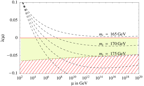
Figure 1: Running of the quartic Higgs coupling for $m_{H}=115~{}{\rm GeV}$ and $m_{t}=165,170,175,180$ and $185~{}{\rm GeV}$ $[\alpha_{s}(m_{Z})=0.118]$. Absolute stability $[\lambda>0]$ is still possible if $m_{t}<166~{}{\rm GeV}$. The hatched region indicates the metastability bound.

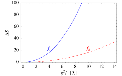
Figure 2: Numerical results for the subtracted part of the correction to the action from top loops $[f_{t}(g_{t}^{2}/|\lambda|)$, solid curve$]$ and gauge boson loops $[f_{g}(g^{2}/|\lambda|)$, dashed curve$]$. Relevant values of $g^{2}/|\lambda|$ are $4\div 8$.

In previous analyses (see e.g. Ref. [12]) a full one-loop computation of the tunnelling rate was never performed, and the semi-classical result was improved by considering only quantum corrections to the effective potential, or to the running of $\lambda$. This procedure leads to a correct estimate of the leading logarithmic corrections to the action, but the finite terms of the calculation are not under control. Within this approximation the use of two-loop RGE equations does not improve the accuracy of the calculation. On the other hand, a consistent implementation of two-loop RGE equations for $\lambda(\mu)$ is possible starting from Eq. (3.2).

In Fig. 1 we plot the evolution of $\lambda(\mu)$ as obtained by integrating the two-loop RGE equations of $\lambda$, the top Yukawa coupling $g_{t}$ and the three gauge couplings $g_{i}$ [13] for $m_{H}=115~{}{\rm GeV}$ and some reference values of the pole top mass $m_{t}$. For comparison we also show the lower bound on $\lambda$ derived from Eq. (3.2), imposing the condition $p<1$ and assuming $V_{U}=(10^{10}~{}{\rm yr})^{4}$. As can be noticed, the evolution of $\lambda$ crosses the metastability bound (i.e. the tunnelling rate becomes too high) for values of $\mu$ much larger than the electroweak scale. This implies that our approximation of neglecting the ${\cal O}(v^{2})$ quadratic term in the tree-level potential is very good, since the critical bounces are those with a size much smaller than $1/v$. It is also important to notice how the lower bound on $\lambda$ increases as a function of the RGE scale (or of $1/R$). This effect is due to the pre-exponential factor in Eq. (3.2), scaling like $R^{-4}$, which we have been able to determine from the one-loop computation. It is important to notice that, for the experimentally interesting values of $m_{H}$ and $m_{t}$, the tunnelling rate is dominated by bubbles with $1/R$ about two orders of magnitude below $\Lambda_{\rm Pl}$, as can be seen in Fig. 1 or, more clearly, in Fig. 3. Therefore the metastability bound on $m_{H}$ does not depend on the unknown physics around $\Lambda_{\rm Pl}$.

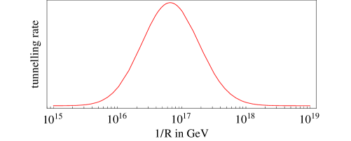
Figure 3: Contribution to the tunnelling rate (in arbitrary units) from bubbles of different $R$, as a function of $1/R$, for $m_{H}=115~{}{\rm GeV}$ and $m_{t}=175~{}{\rm GeV}$.

4 Explicit computation of the one-loop action

4.1 General strategy

The central point in the computation of the tunnelling probability, Eq. (3.1), is the evaluation of ratios of functional determinants:

$$\frac{\mathop{\rm Det}S_{0}^{\prime\prime}[h]}{\mathop{\rm Det}S_{0}^{\prime\prime}[0]}$$ (4.1)

in the various sectors of the theory. This requires solving eigenvalue equations of the type

$$S_{0}^{\prime\prime}[h]\,\psi=[-\partial^{2}+W(r)]\,\psi=\lambda\psi,$$ (4.2)

where $\psi$ generically denotes scalar, fermion or gauge fieds. In order to perform such a calculation, one should i) choose a suitable eigenfunction basis; ii) define the renormalization procedure. In both respects, our approach will be similar to that of Ref. [16], where sphaleron computations within the SM have been performed. Details will be given in the next subsections; here we just sketch the main points of our strategy.

Because of the four-dimensional spherical symmetry of the bounce, the ‘interaction term’ $W$ in (4.2) depends only on the radial coordinate $r=(x_{\mu}x_{\mu})^{1/2}$. For this reason it is convenient to decompose the various fields in eigenstates of the four-dimensional angular momentum operator $L^{2}$, and to write the Laplace operator as

$$\partial^{2}=\partial_{\mu}\partial_{\mu}=\frac{d^{2}}{dr^{2}}+\frac{3}{r}\frac{d}{dr}-\frac{L^{2}}{r^{2}}\equiv\nabla_{L}~{}.$$ (4.3)

In the case of scalar fields, the eigenfunctions of $L^{2}$ are the four-dimensional spherical harmonics $Y_{j}(\theta)$ (where $\theta$ collectively denotes the 3 polar angles) with eigenvalues $4j(j+1)$, and degeneracy $(2j+1)^{2}$, where $j$ takes integer and semi-integer values (see Appendix A). After this decomposition, we have

$$\log\mathop{\rm Det}S_{0}^{\prime\prime}=\sum_{j}\log\mathop{\rm Det}(S_{0}^{\prime\prime})_{j}~{},$$ (4.4)

where $(S_{0}^{\prime\prime})_{j}$ is the restriction of $S_{0}^{\prime\prime}$ to the subspace spanned by eigenfunctions with angular momentum $j$. As we shall see, the situation is slightly more complicated for fermion and vector fields. Their expansion in spinor and vectorial hyperspherical harmonic functions will be obtained starting from the $Y_{j}(\theta)$.

A further simplification arises from the fact that, in order to compute the ratio in Eq. (4.1), it is only necessary to solve Eq. (4.2) for $\lambda=0$. Indeed, we can use the result [17]

$$\rho_{j}\equiv\frac{\mathop{\rm Det}\left[-\nabla_{L}+W(r)\right]}{\mathop{\rm Det}\left[-\nabla_{L}\right]}=\lim_{r\to\infty}\frac{\det u^{j}_{W}(r)}{\det u^{j}_{0}(r)}~{},$$ (4.5)

where $u^{j}_{W}(r)$ [$u^{j}_{0}(r)$] are eigenfunctions, regular at $r=0$, of $-\nabla_{L}+W(r)$ [$\nabla_{L}$] with zero eigenvalues:

$$[-\nabla_{L}+W(r)]\,u^{j}_{W}(r)=0,\qquad\nabla_{L}\,u^{j}_{0}(r)=0~{}.$$ (4.6)

The symbol ‘det’ in Eq. (4.5) stands for the ordinary determinant over residual (spinorial, gauge group, etc.) indices of these solutions (see e.g. [16] and the next subsections for more details).

The one-loop action is affected by the usual ultraviolet divergences of renormalizable quantum field theories. As a consequence, the sum over $j$ in Eq. (4.4) is not convergent (the ultraviolet behaviour being encoded in the behaviour of the determinants for $j\to\infty$), and the usual renormalization procedure is needed. The expression

$$S_{1}=S_{0}+\frac{1}{2}\ln\mathop{\rm SDet}S^{\prime\prime}_{0}[h]-\frac{1}{2}\ln\mathop{\rm SDet}S^{\prime\prime}_{0}[0]\equiv S_{0}+\Delta S$$ (4.7)

can be made finite by adding an appropriate set of local counterterms, which lead to a redefinition of the bare couplings in $S_{0}$. For example, in the $\overline{\rm MS}$ scheme (dimensional regularization with $\overline{\rm MS}$ subtraction) the renormalized one-loop action can be written as

$$S_{1}=S_{0}^{\overline{\rm MS}}+\left[\Delta S-\left(\Delta S\right)_{\rm pole}\right],$$ (4.8)

where $S_{0}^{\overline{\rm MS}}$ is the lowest-order action expressed in terms of the renormalized $\overline{\rm MS}$ couplings, and $\left(\Delta S\right)_{\rm pole}$ is the divergent part of $\Delta S$ defined according to the $\overline{\rm MS}$ renormalization prescription. Computing the full determinant in $d=4-2\epsilon$ dimensions would be an extremely difficult task. However, this is not necessary. In fact, the divergent terms are all contained in $\Delta S^{[2]}$, defined as the expansion of $\Delta S$ up to second order in the ‘interaction’ $W$:

$$\Delta S^{[2]} = \frac{1}{2}\left[\ln\mathop{\rm SDet}\left(-\partial^{2}+W\right)-\ln\mathop{\rm SDet}\left(-\partial^{2}\right)\right]_{{\cal O}(W^{2})}$$ (4.9)

$$= \frac{1}{2}{\rm STr}\left[(-\partial^{2})^{-1}W\right]-\frac{1}{4}{\rm STr}\left[(-\partial^{2})^{-1}W(-\partial^{2})^{-1}W\right]~{},$$

where ${\rm STr}={\rm Tr}$ or ${\rm STr}=-2{\rm Tr}$ depending on whether it acts on boson or fermion fields. In other words, the difference $\Delta S-\Delta S^{[2]}$ is ultraviolet-finite. Equation (4.8) can be rewritten as

$$S_{1}=S_{0}^{\overline{\rm MS}}+\bigg{[}\Delta S-\Delta S^{[2]}\bigg{]}+\bigg{[}\Delta S^{[2]}-\left(\Delta S\right)_{\rm pole}\bigg{]}~{},$$ (4.10)

where the two terms in square brackets are separately finite. The advantage of this last expression is that $\Delta S^{[2]}$ can be computed either as a (divergent) sum of terms corresponding to different values of the angular momentum, which gives a finite result when subtracted from $\Delta S$, or by standard diagrammatic techniques in $4-2\epsilon$ dimensions. In the next subsections we shall show how this procedure is implemented in practice.

The final result is expressed in terms of the renormalized parameters $\lambda,~{}g_{t}$ and $g_{i}$, whose definitions depend on the renormalization scheme. Of course, the scheme dependence disappears once these couplings are re-expressed in terms of physical observables, such as Higgs and top pole masses. In practice, however, in the case of the gauge couplings it turns out to be more convenient to directly use the $\overline{\rm MS}$ definitions, since these parameters are accurately determined by fitting multiple observables.

4.2 Higgs fluctuations

The relative corrections to the action due to fluctuations of the Higgs field are generally small because the Higgs coupling $\lambda$ is small; it is however important to consider them, because they include the special zero-modes (eigenfunctions with zero eigenvalue) corresponding to translations ($j=1/2$) and field dilatations ($j=0$) of the bounce, as well as the unique negative eigenvalue corresponding to space dilatations of the bounce. It is precisely the existence of this negative eigenvalue that makes the false vacuum unstable. In this case the interaction term is simply given by

$$W(r)=V^{\prime\prime}(h)=-\frac{24R^{2}}{(r^{2}+R^{2})^{2}}~{}.$$ (4.11)

It does not depend on any coupling constant, as expected, since the leading contribution to the action is proportional to $1/\lambda$.

The solutions of the ‘free equation’ $\nabla_{L}u_{0}^{j}(r)=0$, regular in $r=0$, are immediately found to be proportional to $r^{2j}$ (see Eq. (4.3)). In order to exploit the result in Eq. (4.5), we must compute the ratio

$$\rho_{j}(r)=\frac{u_{W}^{j}(r)}{u_{0}^{j}(r)}~{}.$$ (4.12)

The functions $\rho_{j}(r)$ obey the differential equations

$$\rho^{\prime\prime}_{j}(r)+\frac{4j+3}{r}\rho^{\prime}_{j}(r)=W(r)~{}\rho_{j}(r)~{},$$ (4.13)

which can be solved analytically:

$$\rho_{j}(r)=\frac{R^{4}+a_{j}r^{2}R^{2}+b_{j}r^{4}}{(r^{2}+R^{2})^{2}}~{},$$ (4.14)

where

$$a_{j}=\frac{2j-1}{j+1};\;\;\;\;b_{j}=\frac{j(2j-1)}{(j+1)(2j+3)}~{}.$$ (4.15)

According to Eq. (4.5), we have therefore

$$\rho_{j}=\frac{\mathop{\rm Det}\left[-\nabla_{L}+W(r)\right]}{\mathop{\rm Det}\left[-\nabla_{L}\right]}=\lim_{r\to\infty}\rho_{j}(r)=b_{j}~{}.$$ (4.16)

Let us neglect for the moment the contributions of $j=0$ and $j=1/2$, for which $\rho_{j}=0$. Taking into account the multiplicities of the sub-determinants, we have

$$\Delta S^{\rm Higgs}_{j>1/2}={1\over 2}\sum_{j>1/2}(2j+1)^{2}\ln\rho_{j}=\sum_{j>1/2}\left[-6j-3-\frac{3}{2j}+\frac{3}{4j^{2}}+\ldots\right]~{}.$$ (4.17)

As discussed in the previous section, we regularize this expression by subtracting from it the terms obtained by solving Eq. (4.13) perturbatively in $W$. Replacing $W$ with $\epsilon W$, we define the coefficients $h_{ij}$ as $\rho_{j}(\epsilon)=1+\epsilon h_{1j}+\epsilon^{2}h_{2j}+{\cal O}(\epsilon^{3})$. These coefficients can be easily determined numerically. The subtracted series is rapidly converging, and in practice the inclusion of the first ten terms already provides an excellent approximation of the full result. We find

$${1\over 2}\sum_{j>1/2}(2j+1)^{2}\ln\rho_{j}-{1\over 2}\sum_{j\geq 0}(2j+1)^{2}\left(h_{1j}-h^{2}_{1j}+\frac{h_{2j}}{2}\right)=12.6~{}.$$ (4.18)

We now turn to a discussion of zero eigenvalues. The four zero-modes in the $j=1/2$ sector correspond to translations of the bounce. They can be converted into a volume factor following the procedure illustrated in [10], which amounts to replacing $\rho_{1/2}$ with

$$\rho^{\prime}_{1/2}=\frac{\mathop{\rm Det}^{\prime}\left(S_{0}^{\prime\prime}[h]\right)_{1/2}}{\mathop{\rm Det}\left(S_{0}^{\prime\prime}[0]\right)_{1/2}}=\lim_{\epsilon\to 0}\frac{\mathop{\rm Det}\big{[}\epsilon+\left(S^{\prime\prime}_{0}[h]\right)_{1/2}\big{]}/\epsilon}{\mathop{\rm Det}\left(S_{0}^{\prime\prime}[0]\right)_{1/2}}~{},$$ (4.19)

and multiplying the expression for the tunnelling probability per unit volume by a factor $\sqrt{S_{0}[h]/2\pi}$ for each of the four translation zero modes. This is the origin of the factor $S_{0}^{2}[h]/(2\pi)^{2}$ in Eq. (3.1), which, in our final result Eq. (3.3), is included in $f_{h}$. The elimination of the four vanishing eigenvalues from $\rho_{1/2}$ provides the dimensional factor $R^{-4}$ in Eq. (3.2). In fact, after numerical integration of the corresponding differential equation, we find

$$\rho^{\prime}_{1/2}=0.041{R^{2}}~{}.$$ (4.20)

As can be see from Eq. (4.15), there is another zero eigenvalue in the $j=0$ sector. It arises from the scale invariance of the tree-level potential: bubbles with different field value $\sim 1/R$ have the same tree-level action. Scale invariance is broken by quantum corrections, which shift the zero eigenvalue by an amount of ${\cal O}[g_{i}^{2}/(4\pi R)^{2}]$. We can therefore compute $\rho_{0}$ by removing the zero eigenvalue from the determinant as in Eq. (4.19), and replacing the zero eigenvalue with a quantity of ${\cal O}[g_{i}^{2}/(4\pi R)^{2}]$ (this small correction can in principle be extracted from the $R$ dependence of the one-loop bounce action [18]). This gives $\rho^{\prime}_{0}\sim-R^{2}$, and

$${1\over 2}\ln|\rho_{0}|\sim{1\over 2}\ln\left|\rho^{\prime}_{0}\frac{g_{t}^{2}}{(4\pi R)^{2}}\right|=-2.5$$ (4.21)

for $\rho^{\prime}_{0}=-R^{2}$ and $g_{t}=1$. Note that $\rho^{\prime}_{0}$ is negative, as it should be because of the instability of the electroweak vacuum [10].

Combining the results in Eqs. (4.18)–(4.21) we finally obtain

$$f_{h}^{(1)}\equiv\left[(\Delta S^{\prime}-4\ln R)-\Delta S^{[2]}\right]_{\rm Higgs}=4\pm 1~{},$$ (4.22)

where the quoted error is entirely ascribable to the uncertainty in Eq. (4.21). In Section 4.4, $f_{h}^{(1)}$ will be combined with analogous contributions generated by Goldstone boson fluctuations to yield the constant $f_{h}$ in Eq. (3.3).

Renormalization

Following the general strategy discussed in Section 4.1, we now proceed to evaluate $\Delta S^{[2]}$ in the $\overline{\rm MS}$ scheme. The explicit $d$-dimensional expression of $\Delta S^{[2]}$, defined in Eq. (4.9), is

$$\left[\Delta S^{[2]}\right]^{d}_{\rm Higgs}=\frac{3\lambda\mu^{4-d}}{2}~{}\Delta_{1}\int d^{d}x~{}h^{2}(x)-\frac{9\lambda^{2}\mu^{2(4-d)}}{4}\int d^{d}x~{}d^{d}y~{}~{}h^{2}(x)\Delta_{2}(x-y)h^{2}(y)~{},$$ (4.23)

where

$$\Delta_{1} = \int\frac{d^{d}k}{(2\pi)^{d}}\frac{1}{k^{2}}~{},$$ (4.24)

$$\Delta_{2}(x-y) = \int\frac{d^{d}q}{(2\pi)^{d}}e^{iq(x-y)}\int\frac{d^{d}k}{(2\pi)^{d}}\frac{1}{k^{2}(k+q)^{2}}~{},$$ (4.25)

and $\mu$ is the usual mass scale that is introduced in dimensional regularization in order to keep the action dimensionless. In dimensional regularization, $\Delta_{1}=0$, and there is thus no contribution to $\Delta S^{[2]}$ from terms of order ${\cal O}(W)$. This is also true for the ${\cal O}(W)$ terms in the fermion and gauge sectors, as a consequence of our approximation of neglecting mass terms in the tree-level potential. The second term in Eq. (4.23) can be written as

$$\left[\Delta S^{[2]}\right]^{d}_{\rm Higgs}=-\frac{9\lambda^{2}\mu^{4-d}}{4}\int\frac{d^{d}q}{(2\pi)^{d}}\left[\widetilde{h^{2}}(q^{2})\right]^{2}B_{0}(q^{2})~{},$$ (4.26)

where $\widetilde{h^{2}}(q^{2})$ is the $d$-dimensional Fourier transform of $h^{2}(x)$ and

$$B_{0}(q^{2})=\mu^{4-d}\int\frac{d^{d}k}{(2\pi)^{d}}\frac{1}{k^{2}(k+q)^{2}}=\frac{1}{(4\pi)^{2}}\left[\frac{1}{\bar{\epsilon}}+2+\ln\frac{\mu^{2}}{q^{2}}\right]+{\cal O}(\bar{\epsilon})~{}.$$ (4.27)

Here $1/\bar{\epsilon}=2/(d-4)-\gamma_{E}+\ln(4\pi)$ denotes the divergent part, to be subtracted according to the $\overline{\rm MS}$ prescription. We therefore have

$$\left(\Delta S\right)_{\rm pole}^{\rm Higgs}=-\frac{1}{\bar{\epsilon}}\,\frac{9\lambda^{2}\mu^{4-d}}{64\pi^{2}}\int\frac{d^{d}q}{(2\pi)^{d}}\left[\widetilde{h^{2}}(q^{2})\right]^{2}~{}.$$ (4.28)

Since

$$\int\frac{d^{d}q}{(2\pi)^{d}}\left[\widetilde{h^{2}}(q^{2})\right]^{2}=\int d^{d}x~{}h^{4}(x)~{},$$ (4.29)

the divergent part in (4.26) is immediately recognized to have the same structure as the bare action.

After subtraction of the $1/\bar{\epsilon}$ pole, the integral in Eq. (4.26) can be safely performed in four dimensions (see Appendix B), leading to

$$\bigg{[}\Delta S^{[2]}-\left(\Delta S\right)_{\rm pole}\bigg{]}_{\rm Higgs}=-\frac{9\lambda^{2}}{64\pi^{2}}\int\frac{d^{4}q}{(2\pi)^{4}}\left[\widetilde{h^{2}}(q^{2})\right]^{2}\left[2+\ln\frac{\mu^{2}}{q^{2}}\right]=-3L-\frac{5}{2}~{},$$ (4.30)

where $L=\ln(R\mu e^{\gamma_{\rm E}}/2)$. Combining the above result with Eq. (4.22), we obtain the full one-loop correction to the action due to fluctuations of the Higgs field, renormalized in the $\overline{\rm MS}$ scheme.

4.3 Top fluctuations

The fermionic determinant due to fluctuations of the top-quark field assumes a form similar to the bosonic one, if expressed in terms of the squared Dirac operator:

$$D/^{\dagger}D/=-\partial^{2}+\left(\frac{g_{t}^{2}}{2}h^{2}+\frac{g_{t}}{\sqrt{2}}\partial/h\right)\equiv-\partial^{2}+W^{2}~{},$$ (4.31)

where $g_{t}$ is the top Yukawa coupling. Indeed, we can write

$$\Delta S_{\rm top}=-\frac{N_{c}}{2}\left[\ln\mathop{\rm Det}\left(D/^{\dagger}D/\right)-\ln\mathop{\rm Det}\left(-\partial^{2}\right)\right],$$ (4.32)

where $N_{c}=3$ is the number of colours.

The only difference with respect to the Higgs case is the structure of $W$. Since $W$ does not commute with $L^{2}$ because of the $\partial/h$ term, we cannot decompose the eigenfunctions as products of scalar spherical harmonics times constant Dirac spinors. However, the spherical symmetry of the bounce, which implies

$$\partial/h(r)={\hat{x}/}h^{\prime}(r)~{},\qquad{\hat{x}}_{\mu}=x_{\mu}/r~{},$$ (4.33)

considerably simplifies the problem. Following Ref. [19], we decompose the fermionic field as

$$\psi(r,\theta)=\sum_{J=\pm 3/2,~{}\pm 5/2,\ldots}\left[\alpha_{1J}(r)\psi_{1J}(\theta)+\alpha_{2J}(r)\psi_{2J}(\theta)\right]~{},$$ (4.34)

where $\alpha_{iJ}(r)$ are scalar functions and $\psi_{iJ}(\theta)$ are spinors written in terms of appropriate hyperspherical harmonic functions of multiplicity $J^{2}-1/4$ (see Appendix A). In this basis the equation $D/^{\dagger}D/\,\psi=0$ becomes

$$\left[\begin{array}[]{cc}-\frac{d^{2}}{dr^{2}}+\frac{J(J-1)}{r^{2}}+\frac{g_{t}^{2}}{2}h^{2}(r)&\frac{g_{t}}{\sqrt{2}}h^{\prime}(r)\\ \frac{g_{t}}{\sqrt{2}}h^{\prime}(r)&-\frac{d^{2}}{dr^{2}}+\frac{J(J+1)}{r^{2}}+\frac{g_{t}^{2}}{2}h^{2}(r)\end{array}\right]\left[\begin{array}[]{c}\alpha_{1J}(r)\\ \alpha_{2J}(r)\end{array}\right]=0~{}.$$ (4.35)

In the limit $g_{t}=0$ the two components of Eq. (4.35) are decoupled; for $J>0$ their solutions, regular in $r=0$, are given by $\alpha^{0}_{1J}\propto r^{J}$ and $\alpha^{0}_{2J}\propto r^{J+1}$. Since Eq. (4.35) is invariant under the exchange $J\leftrightarrow-J$, we shall consider in the following only the case $J>0$, and include an extra factor of 2 in the multiplicity of the solutions. Equation (4.35) can be cast in the form

$$\left\{\begin{array}[]{rcl}\displaystyle\rho^{\prime\prime}_{1J}+2\frac{J}{r}\rho^{\prime}_{1J}&=&\displaystyle\frac{g_{t}^{2}}{2}h^{2}\rho_{1J}+\frac{g_{t}}{\sqrt{2}}h^{\prime}\rho_{2J}r~{},\\[8.53581pt] \displaystyle\rho^{\prime\prime}_{2J}+2\frac{J+1}{r}\rho^{\prime}_{2J}&=&\displaystyle\frac{g_{t}^{2}}{2}h^{2}\rho_{2J}+\frac{g_{t}}{\sqrt{2}}h^{\prime}\rho_{1J}r^{-1}~{},\end{array}\right.$$ (4.36)

where $\rho_{iJ}(r)=\alpha_{iJ}(r)/\alpha^{0}_{iJ}(r)$. The system Eq. (4.36) has two solutions $\rho^{k}_{iJ}(r)$, $k=1,2$ with initial conditions $\rho^{k}_{iJ}(0)=\delta_{ik}$. According to Ref. [17] we can finally write

$$\Delta S_{\rm top}=-3\sum_{J={\rm I\!N}+1/2}\left(J^{2}-\frac{1}{4}\right)\ln\left\{\lim_{r\to\infty}\det\left[\begin{array}[]{cc}\rho^{1}_{1J}(r)&\rho^{2}_{1J}(r)\cr\rho^{1}_{2J}(r)&\rho^{2}_{2J}(r)\end{array}\right]\right\}~{}.$$ (4.37)

The sub-determinants at fixed $J$ can be computed by means of numerical methods. As usual, the sum in Eq. (4.37) is divergent and we regularize it by subtracting the first two powers in $W$. Since $g_{t}$ appears always multiplied by $h(r)$, the final result depends only on the ratio $g^{2}_{t}/|\lambda|$:

$$\bigg{[}\Delta S-\Delta S^{[2]}\bigg{]}_{\rm top}=-f_{t}\left(\frac{g^{2}_{t}}{|\lambda|}\right)~{},$$ (4.38)

and is plotted in Fig. 2 in the range of interest.

The evaluation of $\Delta S^{[2]}$ in dimensional regularization is very similar to the Higgs case. We find

$$\left[\Delta S^{[2]}\right]^{d}_{\rm top}=\frac{N_{c}}{4}\int\frac{d^{d}q}{(2\pi)^{d}}\left\{g_{t}^{4}\mu^{4-d}[\widetilde{h^{2}}(q^{2})]^{2}+2g_{t}^{2}q^{2}{\tilde{h}}^{2}(q^{2})\right\}B_{0}(q^{2})~{},$$ (4.39)

which, after subtraction of the divergent terms, leads to

$$\bigg{[}\Delta S^{[2]}-\left(\Delta S\right)_{\rm pole}\bigg{]}_{\rm top}=\frac{g_{t}^{4}}{6|\lambda|^{2}}\left(5+6L\right)+\frac{g_{t}^{2}}{6|\lambda|}\left(13+12L\right)~{}.$$ (4.40)

4.4 Gauge and Goldstone fluctuations

In order to evaluate quantum fluctuations in the sector of gauge fields we need to modify the bare action introducing an appropriate gauge fixing. Both the correction to the potential and that to the kinetic term are gauge-dependent, but they combine to give gauge-independent physical quantities [20]. For example, at one loop, the divergent corrections change the Higgs action into

$$S=\int d^{4}x\left[(1+Z_{T})|D_{\mu}\phi|^{2}+(1+Z_{V})\lambda|\phi|^{4}\right]~{},$$ (4.41)

and the gauge dependence of $Z_{T}$ and $Z_{V}$ cancels in the combination $Z_{V}-2Z_{T}$ that determines the RGE equation for $\lambda$. By requiring that the bounce action be an extremum under the transformation $h(r)\to h(\xi r)$, one finds that $S_{T}=-2S_{V}$, where $S_{T}$ ($S_{V}$) is the ‘kinetic part’ (‘potential part’) of the tree-level bounce action $S=S_{T}+S_{V}$. Therefore, the divergent corrections to the bounce action are gauge-independent. More generally, it was shown by Nielsen [21] that the value of the effective potential at its minimum is gauge-invariant. Similarly, the value of the effective action is also invariant, when evaluated over a field configuration that extremizes it. It follows that the full corrections to the bounce action are gauge-independent.

The functional obtained after gauge fixing depends on gauge fields $A^{a}_{\mu}$, Goldstone bosons $G^{b}$ and Faddeev–Popov ghosts $\eta^{c}$. We are only interested in the second functional derivative of the action evaluated at $A^{a}_{\mu}=G^{b}=\eta^{c}=0$ and $h\not=0$. This considerably simplifies the problem, since we can ignore the non-Abelian part of gauge interactions. In the following, we will denote with a suffix $A$ the corrections to the action for a generic abelian gauge field $A_{\mu}$, with coupling $g$. We can also ignore the fluctuations of the electromagnetic field: they vanish in the difference $\Delta S[h]-\Delta S[0]$ because the photon field is not coupled to $h$. The problem is thus equivalent to the case of three independent Abelian fields: the two $W$’s and the $Z$.

Introducing a ’t Hooft–Feynman gauge-fixing term, which has proved to be the most convenient choice for our calculation, the relevant part of the bare action can be written as

$$\int d^{4}x~{}\left[\frac{1}{4}F_{\mu\nu}^{2}+\frac{1}{2}(\partial A-ghG)^{2}+|D\phi|^{2}+V(\phi)+\eta^{*}[-\partial^{2}+M(G,h)]\eta\right]~{},$$ (4.42)

where $M(0,h)=g^{2}h^{2}/4$. This choice of the gauge fixing term has the advantage that all terms of the type $A_{\mu}\partial_{\mu}G$ and $\partial_{\mu}\partial_{\nu}A_{\mu}$, generated by $|D\phi|^{2}$ and $F_{\mu\nu}^{2}$, respectively, are eliminated from the equations of motion.

The ghost fields can be treated separately since the the second derivative of the action is diagonal with respect to them. On the contrary, we cannot separate $A_{\mu}$ and $G$, whose zero-eigenvalue equation is given by

$$\left[\begin{array}[]{cc}-\partial^{2}\delta_{\mu\nu}+\frac{1}{4}g^{2}h^{2}(r)\delta_{\mu\nu}&-g\hat{x}_{\mu}h^{\prime}(r)\\ -g\hat{x}_{\nu}h^{\prime}(r)&-\partial^{2}+\left(\frac{1}{4}g^{2}+\lambda\right)h^{2}(r)\end{array}\right]\left[\begin{array}[]{c}A_{\nu}(x)\\ G(x)\end{array}\right]=0~{}.$$ (4.43)

In order to solve Eq. (4.43) we need a suitable decomposition of $A_{\mu}$ in terms of spherical harmonics. A convenient choice is provided by

$$A_{\mu}(x)=\sum_{j=0,\frac{1}{2},1,\ldots}\bigg{[}a_{1j}(r)\hat{x}_{\mu}+\frac{a_{2j}(r)}{2[j(j+1)]^{1/2}}{r\partial_{\mu}}+\sum_{i=3,4}a_{ij}(r)\epsilon_{\mu\nu\rho\sigma}V_{\nu}^{(i)}x_{\rho}\partial_{\sigma}\bigg{]}Y_{j}(\theta)~{},$$ (4.44)

where the $a_{ij}(r)$ are scalar functions and $V_{\nu}^{(i)}$ are two generic orthogonal vectors. In this basis the operator $L^{2}$ is diagonal with respect to the index $j$ and, at fixed $j$, mixes only the first two components, $a_{1j}$ and $a_{2j}$. Since $\partial_{\mu}Y_{0}=0$, the case $j=0$ deserves special attention. For this reason, we discuss separately the two cases $j>0$ and $j=0$.

Sub-determinants with $j>0$

As shown in Appendix A, for $j\not=0$ the zero-eigenvalue equation is

$$\left[\begin{array}[]{ccc}-\nabla_{L}+\frac{3}{r^{2}}+\frac{1}{4}g^{2}h^{2}(r)&-\frac{4\sqrt{j(j+1)}}{r^{2}}&-gh^{\prime}(r)\cr-\frac{4\sqrt{j(j+1)}}{r^{2}}&\!\!\!-\nabla_{L}-\frac{1}{r^{2}}+\frac{1}{4}g^{2}h^{2}(r)&0\cr-gh^{\prime}(r)&0&\!\!\!-\nabla_{L}+(\frac{1}{4}g^{2}+\lambda)h^{2}(r)\end{array}\right]\left[\begin{array}[]{c}a_{1j}(r)\cr a_{2j}(r)\cr G_{j}(r)\end{array}\right]=0~{},$$ (4.45)

$$\left[-\nabla_{L}+\frac{1}{4}g^{2}h^{2}(r)\right]a_{ij}(r)=0~{},\;\;\;\;i=3,4~{},$$ (4.46)

where $G_{j}(r)$ are the components of a standard decomposition of $G(x)$ in spherical harmonics.

Interestingly, the components $a_{3j}$ and $a_{4j}$, which are decoupled from the Goldstone boson sector, obey exactly the same equation as the two components of the complex ghost field. The latter contribute to the action with an opposite sign; therefore these two contributions cancel against each other for $j\not=0$.

Equation (4.45) can be further simplified by means of a rotation in the $(a_{1j},a_{2j})$ space,

$$\left[\begin{array}[]{c}a_{1j}\\ a_{2j}\end{array}\right]=\frac{1}{\sqrt{2j+1}}\left[\begin{array}[]{cc}\sqrt{j}&-\sqrt{j+1}\cr\sqrt{j+1}&\sqrt{j}\end{array}\right]\left[\begin{array}[]{c}{\tilde{a}}_{1j}\\ {\tilde{a}}_{2j}\end{array}\right]~{},\qquad$$ (4.47)

which diagonalizes it in the gauge sector. In this new basis we have

$$\left[\begin{array}[]{ccc}-\nabla_{L_{-}}+\frac{1}{4}g^{2}h^{2}&0&-gh^{\prime}\sqrt{j/(2j+1)}\cr 0&-\nabla_{L_{+}}+\frac{1}{4}g^{2}h^{2}&gh^{\prime}\sqrt{(j+1)/(2j+1)}\cr-gh^{\prime}\sqrt{j/(2j+1)}&gh^{\prime}\sqrt{(j+1)/(2j+1)}&-\nabla_{L}+(\frac{1}{4}g^{2}+\lambda)h^{2}\end{array}\right]\left[\begin{array}[]{c}{\tilde{a}}_{1j}\cr{\tilde{a}}_{2j}\cr G_{j}\end{array}\right]=0~{},$$ (4.48)

where $\nabla_{L_{\pm}}$ denote the usual $\partial^{2}$ operator at fixed angular momentum, with eigenvalues shited by $j\to j\pm 1/2$. The free equation ($h\to 0$) is now diagonal and, similarly to the top and Higgs cases, can be easily solved. We finally obtain

$$\left\{\begin{array}[]{rcl}\displaystyle\rho^{\prime\prime}_{1j}+\frac{1+4j}{r}\rho^{\prime}_{1j}&=&\displaystyle\frac{1}{4}g^{2}h^{2}\rho_{1j}-r\rho_{3j}gh^{\prime}\sqrt{\frac{j}{2j+1}}\\[5.69054pt] \displaystyle\rho^{\prime\prime}_{2j}+\frac{5+4j}{r}\rho^{\prime}_{2j}&=&\displaystyle\frac{1}{4}g^{2}h^{2}\rho_{2j}+\frac{1}{r}\rho_{3j}gh^{\prime}\sqrt{\frac{j+1}{2j+1}}\\[5.69054pt] \displaystyle\rho^{\prime\prime}_{3j}+\frac{3+4j}{r}\rho^{\prime}_{3j}&=&\displaystyle\left(\frac{1}{4}g^{2}h^{2}+\lambda h^{2}\right)\rho_{3j}-\frac{1}{r}\rho_{1j}gh^{\prime}\sqrt{\frac{j}{2j+1}}+r\rho_{2j}gh^{\prime}\sqrt{\frac{j+1}{2j+1}}\end{array}\right.~{},$$ (4.49)

where, as in the previous cases, we have defined

$$\rho_{ij}=\frac{{\tilde{a}}_{ij}}{{\tilde{a}}_{ij}^{0}},\;\;i=1,2;\;\;\;\;\rho_{3j}=\frac{G_{j}}{G_{j}^{0}}~{}.$$ (4.50)

In complete analogy with the top case, the above system has three solutions $\rho^{k}_{ij}(r)$ ($k=1,2,3$), with initial conditions $\rho^{k}_{ij}(0)=\delta_{ik}$, and the resulting correction to the action can be written as

$$\Delta S^{A}_{j>0}=\frac{1}{2}\sum_{j>0}(2j+1)^{2}\ln\left\{\lim_{r\to\infty}\det\left[\begin{array}[]{ccc}\rho^{1}_{1j}(r)&\rho^{2}_{1j}(r)&\rho^{3}_{1j}(r)\cr\rho^{1}_{2j}(r)&\rho^{2}_{2j}(r)&\rho^{3}_{2j}(r)\cr\rho^{1}_{3j}(r)&\rho^{2}_{3j}(r)&\rho^{3}_{3j}(r)\end{array}\right]\right\}~{}.$$ (4.51)

All the determinants in Eq. (4.51) are different from zero and, as usual, their sum must be regularized by the subtraction of $\Delta S^{[2]}$.

Sub-determinant with $j=0$

For $j=0$ only the $\hat{x}_{\mu}$ component of $A_{\mu}$ is different from zero [$A_{\mu}^{(j=0)}=a_{10}(r)\hat{x}_{\mu}$] and the eigenvalue equation is

$$\left[\begin{array}[]{cc}-\frac{d^{2}}{dr^{2}}-\frac{3}{r}\frac{d}{dr}+\frac{3}{r^{2}}+\frac{1}{4}g^{2}h^{2}(r)&-gh^{\prime}(r)\cr-gh^{\prime}(r)&-\frac{d^{2}}{dr^{2}}-\frac{3}{r}\frac{d}{dr}+(\frac{1}{4}g^{2}+\lambda)h^{2}(r)\end{array}\right]\left[\begin{array}[]{c}a_{10}(r)\cr G_{0}(r)\end{array}\right]=0~{}.$$ (4.52)

This leads to

$$\left\{\begin{array}[]{rcl}\displaystyle\rho^{\prime\prime}_{1}+\frac{5}{r}\rho^{\prime}_{1}&=&\displaystyle\frac{1}{4}g^{2}h^{2}\rho_{1}-\frac{1}{r}\rho_{2}gh^{\prime}\\[5.69054pt] \displaystyle\rho^{\prime\prime}_{2}+\frac{3}{r}\rho^{\prime}_{2}&=&\displaystyle\left(\frac{1}{4}g^{2}h^{2}+\lambda h^{2}\right)\rho_{2}-r\rho_{1}gh^{\prime}\end{array}\right.$$ (4.53)

where, as usual, $\rho_{1}=a_{10}/a_{10}^{0}$ and $\rho_{2}=G_{0}/G_{0}^{0}$. The absence of transverse components in $A^{(j=0)}_{\mu}$ implies that the $j=0$ sub-determinant of the ghost fields is not cancelled; it is obtained as the large-$r$ limit of the function $\rho_{\eta}(r)$, where

$$\rho_{\eta}^{\prime\prime}+\frac{3}{r}\rho^{\prime}_{\eta}=\frac{1}{4}g^{2}h^{2}\rho_{\eta}~{}.$$ (4.54)

Employing the usual notation for the two solutions of the system (4.52), we can write

$$\Delta S^{A}_{j=0}=\frac{1}{2}\ln\left\{\lim_{r\to\infty}\det\left[\begin{array}[]{cc}\rho^{1}_{1}(r)&\rho^{2}_{1}(r)\cr\rho^{1}_{2}(r)&\rho^{2}_{2}(r)\end{array}\right]\right\}-\ln\lim_{r\to\infty}\rho_{\eta}(r)~{}.$$ (4.55)

The $2\times 2$ determinant in Eq. (4.55) contains a vanishing eigenvalue. This is present also in the limit $g=0$, and originates from the global symmetry of the action, which persists even after the introduction of the gauge-fixing term. This corresponds to the possibility, for the false vacuum, to tunnel in different directions with equal probabilities. As discussed in [16, 22], the fluctuations corresponding to global rotations can be converted into an integral over the group volume. These zero-mode fluctuations probe the non-abelian structure of the gauge group, so that we can no longer compute separately the $Z,W^{\pm}$ contributions. Considering the full gauge group, we obtain

$$e^{-\Delta S_{\rm gauge}}=16\pi^{2}\bigg{[}\frac{1}{2\pi}\int d^{4}x~{}h^{2}(r)\bigg{]}^{3/2}e^{-\Delta S^{\prime}_{\rm gauge}}\equiv R^{3}e^{-f_{h}^{(2)}-\Delta S^{\prime}_{\rm gauge}}~{},$$ (4.56)

where the factor $16\pi^{2}$ is the volume of the broken $SU(2)$ group. The resulting integral of $h^{2}$ is logarithmically infrared divergent, as a consequence of our approximation of neglecting the mass term in the Higgs potential, which would have acted as an infrared regulator. For this reason, we cut off the integral in Eq. (4.56) at $r=1/v$. The result, for $Rv\ll 1$, is

$$f_{h}^{(2)}=-\frac{3}{2}\ln\left[\frac{2^{17/3}\pi^{7/3}}{|\lambda|}\ln\frac{1}{Rv}\right]+{\cal O}(1/\ln Rv)~{}.$$ (4.57)

This vanishing eigenvalue is the only aspect of our calculation that is sensitive to the infrared behaviour of the potential, and therefore beyond the control of our approximation. However, the sensitivity to the infrared cut-off is mild and does not induce an appreciable numerical uncertainty.

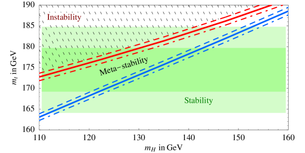
Figure 4: Metastability region of the Standard Model vacuum in the $(m_{H},m_{t})$ plane, for $\alpha_{s}(m_{Z})=0.118$ (solid curves). Dashed and dot-dashed curves are obtained for $\alpha_{s}(m_{Z})=0.118\pm 0.002$. The shaded area indicates the experimental range for $m_{t}$. Sub-leading effects could shift the bounds by $\pm 2~{}{\rm GeV}$ in $m_{t}$.

Once the vanishing eigenvalues have been removed from the $j=0$ sub-determinant, the latter acquires a dimensional factor that is compensated by the factor $R^{3}$ in Eq. (4.56).

Final result for the gauge sector

Summing the regularized gauge and Goldstone corrections, we finally obtain

$$\Delta S_{\rm gauge}=2f_{g}\left(\frac{g_{2}^{2}}{|\lambda|}\right)+f_{g}\left(\frac{g_{Z}^{2}}{|\lambda|}\right)+f_{h}^{(2)}+3f_{h}^{(3)}~{},$$ (4.58)

where

$$f_{h}^{(3)}=\lim_{g\to 0}\left[(\Delta S^{\prime}_{j=0}-\ln R)+\Delta S_{j>0}-\Delta S^{[2]}\right]^{A}\approx 2$$ (4.59)

and

$$f_{g}\Big{(}\frac{g^{2}}{|\lambda|}\Big{)}=\left[(\Delta S^{\prime}_{j=0}-\ln R)+\Delta S_{j>0}-\Delta S^{[2]}\right]^{A}-f_{h}^{(3)}~{},$$ (4.60)

so that $f_{g}(0)=0$. The function $f_{g}$, obtained by means of numerical integration, is plotted in Fig. 2. The constants $f_{h}^{(2)},f_{h}^{(3)}$ can finally be combined with $f_{h}^{(1)}$ in Eq. (4.22) and with the translation prefactors $S_{0}^{2}/(2\pi)^{2}$ to yield

$$f_{h}=f_{h}^{(1)}+f_{h}^{(2)}+3f_{h}^{(3)}-\ln\frac{16\pi^{2}}{9\lambda^{2}}=\frac{7}{2}\ln|\lambda|-8\pm 1~{}.$$ (4.61)

This numerical estimate has been obtained with $Rv=10^{-14}$, but it is very mildly sensitive to the value of $Rv$.

In analogy with the previous cases, dimensional regularization leads to

$$\left[\Delta S^{[2]}\right]^{d}_{A}=-\frac{1}{4}\int\frac{d^{d}q}{(2\pi)^{d}}\bigg{\{}\bigg{[}(d-2)\frac{g^{4}}{16}+\left(\frac{g^{2}}{4}+\lambda\right)^{2}\bigg{]}\mu^{4-d}[\widetilde{h^{2}}(q^{2})]^{2}-2g^{2}q^{2}{\tilde{h}}^{2}(q^{2})\bigg{\}}B_{0}(q^{2})~{},$$ (4.62)

which, after subtraction of the divergent terms, reduces to

$$\bigg{[}\Delta S^{[2]}-\left(\Delta S\right)_{\rm pole}\bigg{]}^{A}=-\frac{5+6L}{18}-\frac{g^{2}}{|\lambda|}\frac{7+6L}{12}-\frac{g^{4}}{\lambda^{2}}\frac{1+2L}{32}.$$ (4.63)

5 Results

Using Eq. (3.2), the condition $p<p_{\rm max}$ can be translated into an upper bound on $|\lambda(\mu)|$:

$$|\lambda(2e^{-\gamma_{E}}/R)| < \frac{8\pi^{2}/3}{\ln(V_{U}/R^{4})-\Delta S-\ln p_{\rm max}}$$ (5.1)

$$= \frac{0.065}{1-\left[\ln(Rv)+\ln(T_{U}^{0}/T_{U})\right]/100-\left[\Delta S+\ln p_{\rm max}\right]/400}~{},\qquad$$

where $\Delta S$ is computed at $L=\ln(R\mu e^{\gamma_{E}}/2)=0$, $V_{U}=T_{U}^{4}$ and $T_{U}^{0}=10^{10}~{}{\rm yr}$. Equation (5.1) must be satisfied for all values of $R$. From this inequality, a lower limit on $m_{H}$ can be obtained by integrating the two-loop RGE equations [13] for $\lambda$, $g_{t}$ and the three gauge couplings $g_{i}$. The initial values of $\lambda$ and $g_{t}$ at $\mu=v$ are related to the values of $m_{H}$ and $m_{t}$ by the matching conditions given in [14] and [15], respectively. As in most recent analyses of the Higgs potential [3], we include the finite two-loop QCD correction in the relation between $g_{t}(m_{t})$ and the top pole mass $m_{t}$. The latter is formally a higher-order contribution, and can be used to estimate the theoretical uncertainty in the determination of $\lambda(\mu)$ at high scales.

Stability and metastability bounds in the $(m_{H},m_{t})$ plane are shown in Fig. 4, which has been obtained with $p_{\rm max}=1$. The metastability condition can be approximated as

$$m_{H}({\rm GeV})>117+2.9\left[m_{t}({\rm GeV})-(175\pm 2)\right]-2.5\left[\frac{\alpha_{s}(m_{Z})-0.118}{0.002}\right]+0.1\ln\left(\frac{T_{U}}{10^{10}~{}{\rm yr}}\right)~{},$$ (5.2)

while the absolute stability bound is given by

$$m_{H}({\rm GeV})>133+2.0\left[m_{t}({\rm GeV})-(175\pm 2)\right]-1.6\left[\frac{\alpha_{s}(m_{Z})-0.118}{0.002}\right]~{}.$$ (5.3)

The numerical impact of $\Delta S$ is rather weak, provided the renormalization scale is chosen such that $L=0$: for $m_{H}=115$ GeV, a correction $\Delta S=50$ shifts the metastability bound by $1~{}{\rm GeV}$ in $m_{t}$. For this reason, our results are numerically close to those obtained in [12] (at zero temperature), where this correction was not included. Note that one could have expected a larger effect, because of the large value of the top Yukawa coupling $g_{t}$ at the weak scale. However, the relevant quantity here is $g_{t}(1/R)$, with $1/R\sim 10^{16}$ GeV, which is substantially smaller than $g_{t}(m_{t})$.

The uncertainties in the determination of $\Delta S$ turn out to be negligible with respect to the uncertainties involved in the determination of $\lambda(\mu)$ at high scales. We estimate the latter to generate an error $\delta m_{t}\sim 2$ GeV at fixed $m_{H}$ and $\alpha_{s}$, both in the stability and metastability bounds, as shown in Eqs. (5.2) and (5.3).

Some comments are in order:

• Vacuum decay can also be catalysed by collisions of cosmic rays. However, it has been shown [23] that the tunnelling rate induced by such processes is negligible with respect to the probability of quantum tunnelling.

• Thermal tunnelling gives stronger bounds than quantum tunnelling only under the assumption that the temperature of the universe has been above $10^{8}-10^{9}$ GeV (for $m_{H}=115$ GeV).

• We have assumed the validity of the Standard Model up to the Planck scale. Experiments at Tevatron run IIB can reduce the error on $m_{t}$ down to $\pm 2~{}{\rm GeV}$ [25] and possibly discover the Higgs and measure its mass if $m_{H}<130$ GeV. Some extension of the SM will become necessary, should $m_{H}$ and $m_{t}$ be found in the excluded region. All concrete modifications invoked to cure this problem give a computable correction to the squared Higgs mass; for example, a scalar with mass $\tilde{m}$ and a coupling $\tilde{\lambda}$ to the Higgs gives $\delta m_{H}^{2}\sim\tilde{\lambda}\tilde{m}^{2}/(4\pi)^{2}$. Since $\tilde{\lambda}$ cannot be too small, by naturalness arguments we expect the scale $\tilde{m}$ of new physics to be in the electroweak range.

• All observed neutrino anomalies could be explained in terms of neutrino oscillations without affecting our result [24].

6 Conclusions

All recent LEP1, LEP2, SLD and Tevatron data are compatible with the Standard Model with $m_{t}\approx 175~{}{\rm GeV}$ and a light Higgs, maybe $m_{H}\approx 115~{}{\rm GeV}$ [5]. It is well known that the Standard Model is affected by the so-called hierarchy problem, which manifests itself through uncomputable quadratically divergent corrections to the Higgs squared mass. The extensions of the theory proposed to cure this potential problem are likely to involve the presence of new phenomena not far above the electroweak scale. However, a definite solution of the naturalness problem is not yet established, and it is interesting to consider the possibility that it be solved by some unknown mechanism that takes place around the Planck scale. Even within this assumption, a possible phenomenological problem affects the SM, namely the possibility that the scalar potential become unbounded from below at large field values, below the Planck scale. For $m_{H}=115~{}{\rm GeV}$ such instability is present if the top mass is larger than $(166\pm 2)~{}{\rm GeV}$, i.e. only about two standard deviations below the central value of the Tevatron data.

The instability of the SM vacuum does not contradict any experimental observation, provided its lifetime is longer than the age of the universe. In semi-classical approximation, this happens if the running quartic Higgs coupling $\lambda$ is larger than about $-0.05$. In this paper we have presented a more accurate assessment of this bound by performing a full next-to-leading order computation of the tunnelling rate of the metastable vacuum. In particular, we have computed the one-loop corrections to the bounce action. Our result is summarized in Eq. (3.3) and plotted in Fig. 4. Next-to-leading corrections turn out to be numerically small, with an appropriate choice of the renormalization scale ($\mu=1/R$), but they allow fixing the various ambiguities of the semi-classical calculation, thus reducing the overall uncertainty of the result. We find that, for $m_{H}=115~{}{\rm GeV}$ (that is, just above the present exclusion limit), the instability is dangerous only for $m_{t}>(175\pm 2)~{}{\rm GeV}$; this result does not depend on the unknown new phyiscs at the Planck scale. A determination of $m_{t}$ at this level of accuracy would therefore be extremely interesting in this respect, and will probably be achieved at Tevatron run II.

Appendix A Spherical harmonics

The spherical harmonics $Y_{jmm^{\prime}}(\theta)$ are eigenfunctions of $L^{2}=L_{\mu\nu}L_{\mu\nu}$, where

$$L_{\mu\nu}=\frac{i}{\sqrt{2}}\left(x_{\mu}\partial_{\nu}-x_{\nu}\partial_{\mu}\right)~{},$$ (A.1)

with eigenvalues $4j(j+1)$; the indices $m,m^{\prime}$ range between $-j$ and $j$ (with $j=0,1/2,1,\ldots$) giving the multiplicity $(2j+1)^{2}$. This multiplicity can be understood by noting that the group of rotations in four dimensions is $O(4)\sim SU(2)\otimes SU(2)$, and its scalar representations correspond to $SU(2)\otimes SU(2)$ representations $(l,k)$ with $l=k$ [26]. The indices $m,m^{\prime}$ will be omitted in the following.

Spin-$1/2$ representations are obtained for $l=k\pm 1/2$. The index $J$ that appears in Eq. (4.34) is related to $l$ and $k$ through

$$J=2k+\frac{3}{2}\qquad {\rm for}\qquad l=k+\frac{1}{2},\;k=0,1/2,1,\ldots~{};$$ (A.2)

$$J=-2k-\frac{1}{2}\qquad {\rm for}\qquad l=k-\frac{1}{2},\;k=1/2,1,\ldots~{}.$$ (A.3)

Therefore, the multiplicity of the representation labelled by $J$ is $(2k+1)(2l+1)=J^{2}-1/4$. The action of the operator $D/$ on the $(l,k)$ spinor representations can be found in Ref. [19].

In the case of vector representations, it is straightforward to work out the action of $\partial^{2}$ on $A_{\mu}(x)$ as in Eq. (4.44). Using Eq. (4.3) we find

$$\partial^{2}a_{1j}\hat{x}_{\mu}Y_{j}(\theta) = \bigg{[}a^{\prime\prime}_{1j}+3\frac{a^{\prime}_{1j}}{r}-a_{1j}\frac{L^{2}+3}{r^{2}}\bigg{]}\hat{x}_{\mu}Y_{j}(\theta)+a_{1j}\frac{2}{r}\partial_{\mu}Y_{j}(\theta)$$ (A.4)

$$\partial^{2}a_{2j}r\partial_{\mu}Y_{j}(\theta) = \bigg{[}a^{\prime\prime}_{2j}+3\frac{a^{\prime}_{2j}}{r}-a_{2j}\frac{L^{2}-1}{r^{2}}\bigg{]}r\partial_{\mu}Y_{j}(\theta)+a_{2j}\frac{2L^{2}}{r^{2}}\hat{x}_{\mu}Y_{j}(\theta)\qquad$$ (A.5)

$$\partial^{2}a_{ij}\epsilon_{\mu\nu\rho\sigma}V_{\nu}^{(i)}x_{\rho}\partial_{\sigma}Y_{j}(\theta) = \bigg{[}a^{\prime\prime}_{ij}+3\frac{a^{\prime}_{ij}}{r}-a_{ij}\frac{L^{2}}{r^{2}}\bigg{]}\epsilon_{\mu\nu\rho\sigma}V_{\nu}^{(i)}x_{\rho}\partial_{\sigma}Y_{j}(\theta)~{}.$$ (A.6)

Therefore, we have

$$\int d^{4}xA_{\mu}\partial^{2}A_{\mu}=\sum_{j}\int r^{3}dr~{}a_{ij}(r)D^{(j)}_{ik}a_{kj}(r)~{},$$ (A.7)

where, with an appropriate normalization of the two vectors $V_{\mu}^{(i)}$,

$$D^{(j)}=\frac{d^{2}}{dr^{2}}+\frac{3}{r}\frac{d}{dr}-\frac{4j(j+1)}{r^{2}}+\left[\begin{array}[]{cccc}-\frac{3}{r^{2}}&\frac{4\sqrt{j(j+1)}}{r^{2}}&0&0\cr\frac{4\sqrt{j(j+1)}}{r^{2}}&\frac{1}{r^{2}}&0&0\cr 0&0&0&0\cr 0&0&0&0\end{array}\right]~{}.$$ (A.8)

Appendix B Fourier transform of the bounce

The four-dimensional Fourier transform of a function $f$, depending only on the radial coordinate $r$, is given by

$${\tilde{f}}(p^{2})\equiv\int d^{4}xe^{ip_{\mu}x_{\mu}}f(r)=\frac{4\pi^{2}}{p}\int_{0}^{\infty}dr\,r^{2}f(r)J_{1}(pr)~{},$$ (B.1)

where $p^{2}=p_{\mu}p_{\mu}$ and

$$J_{1}(pr)=\frac{pr}{\pi}\int_{0}^{\pi}d\theta\,\sin^{2}\theta\,e^{ipr\cos\theta}~{}.$$ (B.2)

In the case of the bounce we find

$${\tilde{h}}(p^{2}) = \frac{4\pi^{2}}{p}\int_{0}^{\infty}dr\,r^{2}h(r)J_{1}(pr)~{}=~{}\frac{8\sqrt{2}\pi^{2}R^{2}K_{1}(pR)}{p\sqrt{|\lambda|}}~{},$$ (B.3)

$$\widetilde{h^{2}}(p^{2}) = \frac{4\pi^{2}}{p}\int_{0}^{\infty}dr\,r^{2}h^{2}(r)J_{1}(pr)~{}=~{}\frac{16\pi^{2}R^{2}}{|\lambda|}K_{0}(pR)~{}.$$ (B.4)

The functions $K_{n}(x)$ and $J_{n}(x)$ are Bessel functions defined as in Mathematica [27].

References

- [1] N. Cabibbo, L. Maiani, G. Parisi and R. Petronzio, Nucl. Phys. B 158 (1979) 295; P.Q. Hung, Phys. Rev. Lett. 42 (1979) 873; M. Lindner, Z. Phys. C 31 (1986) 295; M. Lindner, M. Sher and H. Zaglauer, Phys. Lett. B 228 (1989) 139.
- [2] M. Sher, Phys. Rep. 179 (1989) 273; B. Schrempp and M. Wimmer, Prog. Part. Nucl. Phys. 37 (1996) 1.
- [3] M. Sher, Phys. Lett. B 317 (1993) 159; addendum ibid. 331 (1994) 448; G. Altarelli and G. Isidori, Phys. Lett. B 337 (1994) 141; J.A. Casas, J.R. Espinosa and M. Quirós, Phys. Lett. B 342 (1995) 171; T. Hambye and K. Riesselmann, Phys. Rev. D 55 (1997) 7255.
- [4] P. Abreu et al. [DELPHI Collaboration], Phys. Lett. B 499 (2001) 23; G. Abbiendi et al. [OPAL Collaboration], Phys. Lett. B 499 (2001) 38; P. Igo-Kemenes, LEPC presentation, Nov. 3, 2000, http://lephiggs.web.cern.ch/LEPHIGGS/talks/index.html.
- [5] R. Barate et al. [ALEPH Collaboration], Phys. Lett. B 495 (2000) 1; M. Acciarri et al. [L3 Collaboration], Phys. Lett. B 495 (2000) 18.
- [6] LEP Electroweak Working Group, http://www.web.cern.ch/LEPEWWG.
- [7] The case has been considered in D.L. Bennett, H.B. Nielsen and I. Picek, Phys. Lett. B 208 (1988) 275; C.D. Froggatt and H.B. Nielsen, Phys. Lett. B 368 (1996) 96.
- [8] S. Coleman, Phys. Rev. D 15 (1977) 2929.
- [9] K. Lee and E.J. Weinberg, Nucl. Phys. B 267 (1986) 181.
- [10] C.G. Callan and S. Coleman, Phys. Rev. D 16 (1762) 1977.
- [11] J. Langer, Ann. Phys. 41 (1967) 108 ; ibid. 54 (1969) 258 ; Physica 73 (1974) 61 .
- [12] J.R. Espinosa and M. Quiros, Phys. Lett. B 353 (1995) 257.
- [13] C. Ford, D.R. Jones, P.W. Stephenson and M.B. Einhorn, Nucl. Phys. B 395 (1993) 17.
- [14] A. Sirlin and R. Zucchini, Nucl. Phys. B 266 (1986) 389.
- [15] R. Hempfling and B.A. Kniehl, Phys. Rev. D 51 (1995) 1386.
- [16] J. Baacke and S. Junker, Phys. Rev. D 49 (1994) 2055; ibid. 50 (1994) 4227.
- [17] S. Coleman, “The uses of instantons”, Lecture delivered at 1977 Int. School of Subnuclear Physics, Erice, Italy, 1977; R. Dashen, B. Hasslacher and A. Neveu, Phys. Rev. D 10 (1974) 4114.
- [18] I. Affleck, Nucl. Phys. B 191 (1981) 429.
- [19] J. Avan and H.J. De Vega, Nucl. Phys. B 269 (1986) 621.
- [20] J.-M. Frère and P. Nicoletopoulos, Phys. Rev. D 11 (1975) 2332.
- [21] N.K. Nielsen, Nucl. Phys. B 101 (1975) 173.
- [22] A. Kusenko, K. Lee and E.J. Weinberg, Phys. Rev. D 55 (1997) 4903.
- [23] K. Enqvist and J. McDonald, Nucl. Phys. B 513 (1998) 661.
- [24] F. Vissani, Phys. Rev. D 57 (1998) 7027.
- [25] G. Brooijmans (for the CDF and D0 collaborations), hep-ex/0005030.
- [26] M. Daumens and P. Minnaert, J. Math. Phys. 17 (1976) 2085.
- [27] S. Wolfram, The Mathematica book, 3rd ed. (Wolfram Media/Cambridge Univ. Press, 1996).