hep-ph/0103333

LMU 01/05

Electroweak D-Waves

Xavier Calmet

and

Harald Fritzsch

Ludwig-Maximilians-University Munich, Sektion Physik
Theresienstraße 37, D-80333 Munich, Germany

We consider phenomenological implications of a model recently proposed for the electroweak interactions based on a $SU(2)_{L}$ confining theory. We concentrate on the production of excited states of the electroweak bosons at future colliders and we consider their contribution to the reaction $W^{+}+W^{-}\to W^{+}+W^{-}$. We expect large deviations from the standard model in the TeV region.

1 Introduction

The aim of this work is to investigate the phenomenological implications of a model recently proposed for the electroweak interactions based on a $SU(2)_{L}$ confining theory [1]. We shall concentrate on orbital and radial excitations of the electroweak bosons. Our model makes use of the confinement mechanism proposed in Ref. [2]. It was emphasized in Ref.[3] that models of a similar class imply different search strategies for the Higgs boson than those usually adopted when searching for the standard model, supersymmetric or fermiophobic Higgs bosons.

In our model the left-handed particles appear as bound states of fundamental, unobservable fermions $f_{L}$ and $q_{L}$ and a scalar $h$. These particles transform as doublets under $SU(2)_{L}$. Besides this, $q_{L}$ is a triplet under $SU(3)_{c}$. We can then identify the following physical left-handed fermions, Higgs boson and electroweak bosons.

$$\begin{array}[]{lllllll}\mbox{neutrino:}&\nu_{L}&\rightarrow&\bar{h}l&\\ \mbox{electron:}&e_{L}&\rightarrow&hl&\\ \mbox{up type quark:}&u_{L}&\rightarrow&\bar{h}q&\\ \mbox{down type quark:}&d_{L}&\rightarrow&hq&\\ \mbox{Higgs particle:}&\phi&\rightarrow&\bar{h}h&(\mbox{$s$-wave})\\ \mbox{$W^{3}$ boson:}&W^{3}&\rightarrow&\bar{h}h&(\mbox{$p$-wave})\\ \mbox{$W^{-}$ boson:}&W^{-}&\rightarrow&hh&(\mbox{$p$-wave})\\ \mbox{$W^{+}$ boson:}&W^{+}&\rightarrow&(hh)^{\dagger}&(\mbox{$p$-wave}),\end{array}$$ (9)

assuming a $SU(2)_{L}$ confinement. The right-handed particles are those of the standard model. In our approach the electroweak bosons appear as excited states of the Higgs boson. It was shown in Ref.[1] that the minimal sector of the model, i.e., the sector containing only the particles predicted by the standard model, is identical to the standard model [4] if one chooses the unitary gauge, we call this property duality. This is done by fixing the gauge and performing a $1/F$ expansion, where $F\cong 492$ GeV is the scale of the theory. In this model new particles corresponding to exotic particles like leptoquarks can be introduced. But, they do not obey to this expansion, and the duality cannot be applied to describe their properties. Forces between two fermions can be very much different than those between a fermion and a scalar or between two scalars. If leptoquarks do exist, their mass scale is presumably very high.

Of particular interest are radially excited versions of the Higgs boson $H^{*}$ and of the electroweak bosons $W^{3*}$ and $W^{\pm*}$. As described in [1], the most promising candidates for energies available at the LHC or at future linear colliders are the excited states of the Higgs boson and of the electroweak bosons. Especially the orbital excitation, i.e., the spin 2 $d$-waves $D^{3}_{\mu\nu}$, $D^{-}_{\mu\nu}$ and $D^{+}_{\mu\nu}$, of the electroweak bosons have a well defined $1/F$ expansion (we use the unitary gauge: $h=(h_{(1)}+F,0)$:

$$D^{3}_{\mu\nu} = \frac{2}{g^{2}F^{2}}\left(\left(D_{\mu}h\right)^{\dagger}\left(D_{\nu}h\right)+\left(D_{\nu}h\right)^{\dagger}\left(D_{\mu}h\right)\right)\approx b^{3}_{\nu}b^{3}_{\mu}+b^{+}_{\nu}b^{-}_{\mu}+b^{+}_{\mu}b^{-}_{\nu}$$ (10)

$$D^{-}_{\mu\nu} = \frac{-\sqrt{2}}{g^{2}F^{2}}\epsilon^{ij}\left(\left(D_{\mu}h\right)_{i}\left(D_{\nu}h\right)_{j}+\left(D_{\nu}h\right)_{i}\left(D_{\mu}h\right)_{j}\right)\approx b^{3}_{\mu}b^{-}_{\nu}+b^{3}_{\nu}b^{-}_{\mu}$$

$$D^{+}_{\mu\nu} = \left(\frac{-\sqrt{2}}{g^{2}F^{2}}\epsilon^{ij}\left(\left(D_{\mu}h\right)_{i}\left(D_{\nu}h\right)_{j}+\left(D_{\nu}h\right)_{i}\left(D_{\mu}h\right)_{j}\right)\right)^{\dagger}\approx b^{3}_{\mu}b^{+}_{\nu}+b^{3}_{\nu}b^{+}_{\mu}$$

where $D_{\mu}$ is the covariant derivative, $b_{\mu}^{a}$, $a=\{3,+,-\}$ are the gauge fields and $g$ the coupling constant corresponding to the gauge group $SU(2)_{L}$. Although the masses and the couplings of these electroweak $d$-waves to other particles are fixed by the dynamics of the model, it is difficult to determine these parameters. In analogy to Quantum Chromodynamics, it is expected that these $d$-waves couple with a reasonable strength to the corresponding $p$-waves, the electroweak bosons. In the following, we assume in accordance with the duality property, that the $d$-waves only couple to the electroweak bosons and not to the photon, Higgs boson or the fermions.

2 Production of the electroweak $d$-waves

The cross-sections and decay width of $d$-waves predicted in a variety of composite models were considered in Ref.[5]. Here we shall consider different effective couplings of our electroweak $d$-waves that are more suitable for the model proposed in [1]. If their masses are of the order of the scale of the theory, they will be accessible at the LHC. Of particular interest is the neutral electroweak $d$-wave because it is expected to couple to the $W^{\pm}$ electroweak bosons. This particle can thus be produced by the fusion of two electroweak bosons at the LHC or at linear colliders.

We shall use the formalism developed by van Dam and Veltman [6] for massive $d$-waves to compute the decay width of the $D^{3}_{\mu\nu}$ into $W^{+}W^{-}$. We use the following relation:

$$\sum^{5}_{i=1}e^{i}_{\mu\nu}(p)e^{i}_{\alpha\beta}(p) = \frac{1}{2}\left(\delta_{\mu\alpha}\delta_{\nu\beta}+\delta_{\mu\beta}\delta_{\nu\alpha}-\delta_{\mu\nu}\delta_{\alpha\beta}\right)$$

$$+\frac{1}{2}\left(\delta_{\mu\alpha}\frac{p_{\nu}p_{\beta}}{m_{D}^{2}}+\delta_{\nu\beta}\frac{p_{\mu}p_{\alpha}}{m_{D}^{2}}+\delta_{\mu\beta}\frac{p_{\nu}p_{\alpha}}{m_{D}^{2}}+\delta_{\nu\alpha}\frac{p_{\mu}p_{\beta}}{m_{D}^{2}}\right)$$

$$+\frac{2}{3}\left(\frac{1}{2}\delta_{\mu\nu}-\frac{p_{\mu}p_{\nu}}{m_{D}^{2}}\right)\left(\frac{1}{2}\delta_{\alpha\beta}-\frac{p_{\alpha}p_{\beta}}{m_{D}^{2}}\right)$$

for the sum over the polarizations $e^{i}_{\mu\nu}$ of the $d$-wave. In the notation of Ref.[6] the sum over the polarizations of the $W^{\pm}$ is given by

$$\sum^{3}_{i=1}e^{i}_{\mu}(p)e^{i}_{\nu}(p) = \delta_{\mu\nu}+\frac{p_{\mu}p_{\nu}}{m_{W}^{2}}$$ (12)

where $\delta_{\mu\nu}$ is the Euclidean metric. Averaging over the polarizations of the $d$-wave, we obtain

$$\Gamma(D^{3}\rightarrow W^{+}W^{-}) = \frac{g^{2}_{D}}{1920m_{D}\pi}\left(x_{W}-4\right)^{2}\sqrt{\left(1-\frac{4}{x_{W}}\right)}$$ (13)

with $x_{W}=(m_{D}/m_{W})^{2}$, where $m_{D}$ is the mass of the $d$-wave and $g_{D}$ is a dimensionfull coupling constant with $\mbox{dim}[g_{D}]=\mbox{GeV}$. A dimensionless coupling constant is obtained by a redefinition of the coupling constant $g_{D}\rightarrow m_{D}\bar{g}_{D}$. We shall discuss plausible numerical inputs in the next section. Assuming that the $Z$ boson couples with the same strength to the $d$-wave as the $W$-bosons, we can approximate the decay width into $Z$ bosons in the following way

$$\Gamma(D^{3}\rightarrow ZZ) = \frac{g^{2}_{D}}{3840m_{D}\pi}\left(x_{Z}-4\right)^{2}\sqrt{\left(1-\frac{4}{x_{Z}}\right)}$$

$$\approx \frac{1}{2}\Gamma(D^{3}\rightarrow W^{+}W^{-})$$

with $x_{Z}=(m_{D}/m_{Z})^{2}$. The Breit-Wigner resonance cross section for the reaction $W^{+}+W^{-}\rightarrow D^{3}$ thus reads (see e.g. [7])

$$\sigma^{(res)}_{W^{+}+W^{-}\rightarrow D^{3}} = \frac{10\pi}{q^{2}}\frac{m_{D}^{2}\Gamma^{\mbox{(tot)}}_{D}\Gamma(D^{3}\rightarrow W^{+}W^{-})}{\left(m_{D}^{2}-s\right)^{2}+m_{D}^{2}{\Gamma^{\mbox{(tot)}}_{D}}^{2}}$$ (15)

where $q^{2}=(s-4m_{W}^{2})/4$ and $\Gamma^{(\mbox{tot})}_{D}\approx 3/2\Gamma(D^{3}\rightarrow W^{+}W^{-})$ is the total decay width of the neutral $d$-wave. Due to the background, the $W$ bosons might be difficult to observe. But, if the electroweak $d$-waves states are produced we expect an excess of $Z$ bosons compared to the standard model expectation. Note that the $Z$ bosons are easier to observe.

As we shall see in the next section, the neutral $d$-waves give a sizable contribution to the reaction $W^{+}+W^{-}\to W^{+}+W^{-}$.

3 The reaction $W^{+}+W^{-}\to W^{+}+W^{-}$

A considerable attention has been paid to the scattering of electroweak bosons since this represents a stringent test of the gauge structure of the standard model. In particular the reaction $W^{+}+W^{-}\to W^{+}+W^{-}$ is known to be of prime interest. If the Higgs boson is heavier than 1 TeV, the electroweak bosons will start to interact strongly [8]. This reaction has been studied in the framework of the standard model in Ref. [9] and the one loop corrections were considered in [10] and are known to be sizable. For the sake of this paper the tree level diagrams are sufficient to show that the contribution of the neutral electroweak $d$-wave will have a considerable impact to that reaction and cannot be overlooked in forthcoming experiments. As described in [11] (see also Ref. [9]) the $W$’s emitted by the beam particles are dominantly longitudinally polarized if the following relations are fulfilled: $m_{W}^{2}\ll m^{2}_{WW}\ll s$ at an $e^{+}$ $e^{-}$ collider, and $m_{W}^{2}\ll m^{2}_{WW}\ll s_{q\bar{q}}\ll s$ at a hadron collider, and we shall only consider the especially interesting reaction $W^{+}_{L}+W^{-}_{L}\to W^{+}_{L}+W^{-}_{L}$ as described in [9].

In the standard model, this reaction is a test of the gauge structure of the theory [12]. The Feynman graphs contributing in the standard model to this reaction can be found in figures 3, 3, 3, 5 and 5.

Figure 1: photon and Z boson in the s channel

Figure 2: photon and Z boson in the t channel

Figure 3: four W vertex

Figure 4: Higgs boson in the s channel

Figure 5: Higgs boson in the t channel

The amplitudes corresponding to these graphs are [9]

$$A_{s\gamma} = -\frac{1}{16}ig^{2}xs^{2}\beta^{2}(3-\beta^{2})^{2}\cos{\theta},$$ (16)

$$A_{sZ} = -\frac{1}{16}ig^{2}(1-x)\frac{s^{3}}{s-\xi_{Z}}\beta^{2}(3-\beta^{2})^{2}\cos{\theta},$$

$$A_{t\gamma} = -\frac{1}{32}ig^{2}x\frac{s^{3}}{t}[\beta^{2}(4-2\beta^{2}+\beta^{4})+\beta^{2}(4-10\beta^{2}+\beta^{4})\cos{\theta}$$

$$+(2-11\beta^{2}+10\beta^{4})\cos^{2}{\theta}+\beta^{2}\cos^{3}{\theta}],$$

$$A_{tZ} = -\frac{1}{32}ig^{2}(1-x)\frac{s^{3}}{t-\xi_{Z}}[\beta^{2}(4-2\beta^{2}+\beta^{4})+\beta^{2}(4-10\beta^{2}+\beta^{4})\cos{\theta}$$

$$+(2-11\beta^{2}+10\beta^{4})\cos^{2}{\theta}+\beta^{2}\cos^{3}{\theta}],$$

$$A_{4} = -\frac{1}{16}ig^{2}s^{2}(1+2\beta^{2}-6\beta^{2}\cos{\theta}-\cos^{2}{\theta}),$$

$$A_{sH} = -\frac{1}{16}ig^{2}s^{2}\frac{(1+\beta^{2})^{2}}{s-\xi_{H}+i\gamma_{H}},$$

$$A_{tH} = -\frac{1}{16}ig^{2}s^{2}\frac{(\beta^{2}-\cos{\theta})^{2}}{t-\xi_{H}+i\gamma_{H}},$$

where $x=\sin^{2}{\theta_{W}}$, $\xi_{Z}=(1-x)^{-1}=m_{Z}^{2}/m^{2}_{W}$, $\xi_{H}=m_{H}^{2}/m^{2}_{W}$, $\gamma_{H}=m_{H}\Gamma_{H}/m_{W}^{2}$ and $\beta=\sqrt{1-4/s}$. The variables $s$ and $t$ are scaled with respect to $m_{W}^{2}$. The scattering angle is $\theta$, $t=-1/2s\beta^{2}(1-\cos{\theta})$. These notations are the same as those introduced in Ref.[9]. The standard model amplitude is thus

$$A^{sum}_{SM} = A_{s\gamma}+A_{sZ}+A_{t\gamma}+A_{tZ}+A_{4}+A_{sH}+A_{tH}.$$ (17)

In the high energy limit, one observes the cancellation of the leading powers in $s$ and finds [9]

$$A^{sum}_{SM}\approx\frac{1}{2}ig^{2}\left[\xi_{Z}\left(1+\frac{s}{t}+\frac{t}{s}\right)+\xi_{H}-i\gamma_{H}\right]$$ (18)

for the sum of these amplitudes. The cross section with the angular cut $-z_{0}<\cos\theta<z_{0}$ is then

$$\sigma = \frac{1}{16\pi s^{2}\beta^{2}}\int^{t_{+}}_{t_{-}}|A^{sum}|^{2}\mbox{d}t$$ (19)

in dimensionless units, $t_{\pm}=(2-s/2)(1\mp z_{0})$.

The excitations of the Higgs and electroweak bosons also contribute via the $s$ and $t$ channel. The amplitudes corresponding to the contribution of a radially excited Higgs boson ($H^{*}$) of mass $m_{H^{*}}$ and decay width $\Gamma_{H^{*}}$ to this reaction are

$$A_{sH^{*}} = -\frac{1}{16}ig^{2}_{H^{*}}s^{2}\frac{(1+\beta^{2})^{2}}{s-\xi_{H^{*}}+i\gamma_{H^{*}}},$$ (20)

$$A_{tH^{*}} = -\frac{1}{16}ig^{2}_{H^{*}}s^{2}\frac{(\beta^{2}-\cos{\theta})^{2}}{t-\xi_{H^{*}}+i\gamma_{H^{*}}},$$

where $\xi_{H^{*}}=m_{H^{*}}^{2}/m^{2}_{W}$, $\gamma_{H^{*}}=m_{H^{*}}\Gamma_{H^{*}}/m_{W}^{2}$ and $g_{H^{*}}$ is the strength of the coupling between two $W$ bosons and the $H^{*}$ scalar particle.

We shall now consider the contribution of the radially $(W^{3*})$ and orbitally $(D^{\mu\nu})$ excited neutral $Z$ boson. The amplitudes for the $W^{3*}$ can be at once deduced from those of the standard model contribution of the $Z$ boson

$$A_{sW^{3*}} = -\frac{1}{16}ig^{2}_{W^{3*}}\frac{s^{3}}{s-\xi_{W^{3*}}+i\gamma_{W^{3*}}}\beta^{2}(3-\beta^{2})^{2}\cos{\theta},$$ (21)

$$A_{tW^{3*}} = -\frac{1}{32}ig^{2}_{W^{3*}}\frac{s^{3}}{t-\xi_{W^{3*}}+i\gamma_{W^{3*}}}[\beta^{2}(4-2\beta^{2}+\beta^{4})$$

$$+\beta^{2}(4-10\beta^{2}+\beta^{4})\cos{\theta}+(2-11\beta^{2}+10\beta^{4})\cos^{2}{\theta}+\beta^{2}\cos^{3}{\theta}],$$

where $\xi_{W^{3*}}=m_{W^{3*}}^{2}/m^{2}_{W}$, $\gamma_{W^{3*}}=m_{W^{3*}}\Gamma_{W^{3*}}/m_{W}^{2}$ and $g_{W^{3*}}$ is the strength of the coupling between two $W$ bosons and the $W^{3*}$ boson.

The orbitally excited $Z$ boson $(D^{\mu\nu})$ is a $d$-wave, and its propagation is thus described by a propagator corresponding to a massive spin 2 particle. The propagator of a massive spin two particle is as follows (see Ref. [6]):

$$\Gamma_{\mu\nu\rho\sigma} = \frac{1}{p^{2}-m_{D}^{2}}\frac{1}{2}(g_{\mu\rho}g_{\nu\sigma}+g_{\mu\sigma}g_{\nu\rho}-\frac{2}{3}g_{\mu\nu}g_{\rho\sigma})$$ (22)

and we assume that the vertex $W^{+\mu}W^{-\nu}D_{\mu\nu}$ is of the form $ig_{D}$. We obtain the following amplitudes for the $s$ and $t$ channel exchange

$$A_{sD} = \frac{-1}{48}ig_{D}^{2}\frac{m_{D}^{2}}{m_{W}^{2}}\frac{s^{2}}{s-\xi_{D}+i\gamma_{D}}\left(2\beta^{4}+3\cos^{2}{\theta}-2\beta^{2}-1\right)$$ (23)

$$\!\!\!\!\!\!\!\!\!A_{tD} = \frac{-1}{96}ig_{D}^{2}\frac{m_{D}^{2}}{m_{W}^{2}}\frac{s^{2}}{t-\xi_{D}+i\gamma_{D}}\left(4\beta^{4}+6\beta^{2}+3+10\beta^{2}\cos{\theta}+1\cos{\theta}^{2}\right)$$ (24)

Since there is a pole in the $t$ channel whose origin is the photon exchange, one has to impose cuts on the cross sections. For the numerical evaluation of the cross section, we impose a cut of $10^{\circ}$, which is the cut chosen in Ref. [10]. The spin of the particle can be determined from the angular distribution of the cross section. We have neglected the decay width of the $Z$ boson and that of the Higgs boson since we assume that the energy of the process is such that no $Z$ boson or Higgs resonance appear. For numerical estimates, we took $m_{H}=100$ GeV.

We have considered only the reaction involving longitudinally polarized $W$. The amplitudes for different polarizations for the standard model can be found in the literature [9]. The amplitudes for a $H^{*}$ or a $W^{3*}$ can be deduced from the standard model calculations by replacing the masses, the decay widths and the coupling constants. Those for the neutral $d$-wave can be easily calculated using

$${\cal A}^{p_{1}p_{2}p_{3}p_{4}}_{s} = -ig_{D}^{2}\frac{m_{D}^{2}}{m_{W}^{2}}\frac{1}{s-\xi_{D}+i\gamma_{D}}$$

$$\frac{1}{2}\epsilon^{\mu}(p_{1})\epsilon^{\nu}(p_{2})(g_{\mu\rho}g_{\nu\sigma}+g_{\mu\sigma}g_{\nu\rho}-\frac{2}{3}g_{\mu\nu}g_{\rho\sigma})\epsilon^{*\rho}(p_{3})\epsilon^{*\sigma}(p_{4})$$

and

$${\cal A}^{p_{1}p_{2}p_{3}p_{4}}_{t} = -ig_{D}^{2}\frac{m_{D}^{2}}{m_{W}^{2}}\frac{1}{t-\xi_{D}+i\gamma_{D}}$$

$$\frac{1}{2}\epsilon^{\mu}(p_{1})\epsilon^{\rho}(p_{2})(g_{\mu\rho}g_{\nu\sigma}+g_{\mu\sigma}g_{\nu\rho}-\frac{2}{3}g_{\mu\nu}g_{\rho\sigma})\epsilon^{*\nu}(p_{3})\epsilon^{*\sigma}(p_{4})$$

where $p_{i}$ stands for the polarization and also using the following relations

$$\epsilon^{\mu}_{1}(0)=(-p,0,0,E)/m_{W} \epsilon^{\mu}_{1}(\pm)=(0,-1,\pm i,0)/\sqrt{2}$$

$$\epsilon^{\mu}_{2}(0)=(-p,0,0,-E)/m_{W} \epsilon^{\mu}_{2}(\pm)=(0,1,\pm i,0)/\sqrt{2}$$

$$\epsilon^{*\mu}_{3}(0)=(p,-E\sin{\theta},0,-E\cos{\theta})/m_{W} \epsilon^{*\mu}_{3}(\pm)=(0,-\cos{\theta},\mp i,\sin{\theta})/\sqrt{2}$$

$$\epsilon^{*\mu}_{4}(0)=(p,E\sin{\theta},0,E\cos{\theta})/m_{W} \epsilon^{*\mu}_{4}(\pm)=(0,\cos{\theta},\mp i,-\sin{\theta})/\sqrt{2}$$

valid in the center of mass system where $E$ is the energy of the $W$ bosons, $p=\sqrt{E^{2}-m_{W}^{2}}$ is their momentum and $\theta$ is the scattering angle.

4 Discussion

The differential decay widths for the reaction $W_{L}^{+}W_{L}^{-}\to W_{L}^{+}+W_{L}^{-}$ can be found in figure 6 for the reaction involving the neutral $d$-wave, figure 7 for that involving the $W^{3*}$ spin 1 boson and figure 8 for that involving the $H^{*}$ scalar. The particles $W^{3*}$ and $H^{*}$ are assumed to couple, in a first approximation, only to the $W$’s. This allows to compute their decay rates using standard model formulas. As mentioned previously it is not an easy task to predict the mass spectrum of the model, thus we assumed, for numerical illustration, three different masses: 350 GeV, 500 GeV and 800 GeV. The coupling constants are assumed to sizable (see figures). If the cross sections are extrapolated to very high energies, the unitarity is violated. However, as expected in any substructure models, it will be restored by bound states effects.

It is very instructive to plot the ratio of the differential cross section involving new physics to the standard model differential cross section. We have done so for the neutral $d$-wave (Ref. 9). It is obvious from this picture that any deviation from the standard model, even at high energy will manifest it-self already in a deviation from one for that ratio. Already at an energy which is low compared to the mass of the new particle, i.e. well bellow the resonance, one observes a deviation from unity.

Nevertheless the calculation of the full reaction e.g. $e^{+}e^{-}\to W^{+}W^{-}\nu\bar{\nu}$ involves the convolution of the cross section of the reaction $W^{+}W^{-}\to W^{+}+W^{-}$ with functions describing the radiative emission of the $W$’s from the fermions. When this integral is performed some sensitivity is lost. Nevertheless the effects are expected to be so large that they cannot be overlooked. The reaction will allow to test a mass range of a few TeV’s so that even if the new particles are too massive to be produced on-shell, their effects will be noticeable at future colliders.

Figure 6: Dimensionless cross section of the reaction $W_{L}^{+}W_{L}^{-}\to W_{L}^{+}+W_{L}^{-}$ including the d-wave. The solid line is the standard model cross section, the dotted line corresponds to a d-wave of mass 350 GeV, with $\Gamma=4.38$ GeV and $\bar{g}_{W^{3*}}=0.8g$, the long dashed line to a d-wave of mass 500 GeV, with $\Gamma=27.49$ GeV and $\bar{g}_{W^{3*}}=0.7g$ and the dot-dashed line to a d-wave of mass 800 GeV, with $\Gamma=251.03$ GeV and $\bar{g}_{W^{3*}}=0.6g$.

Figure 7: Dimensionless cross section of the reaction $W_{L}^{+}W_{L}^{-}\to W_{L}^{+}+W_{L}^{-}$ including the $W^{3*}$ boson. The solid line is the standard model cross section, the dotted line corresponds to a $W^{3*}$ boson of mass 350 GeV, with $\Gamma=66.2$ GeV and $\bar{g}_{W^{3*}}=0.8\sin^{2}{\theta_{W}}g$, the long dashed line to a $W^{3*}$ boson of mass 500 GeV, with $\Gamma=266.8$ GeV and $\bar{g}_{W^{3*}}=0.7\sin^{2}{\theta_{W}}g$ and the dot-dashed line to a $W^{3*}$ boson of mass 800 GeV, with $\Gamma=1795.5$ GeV and $\bar{g}_{W^{3*}}=0.6\sin^{2}{\theta_{W}}g$.

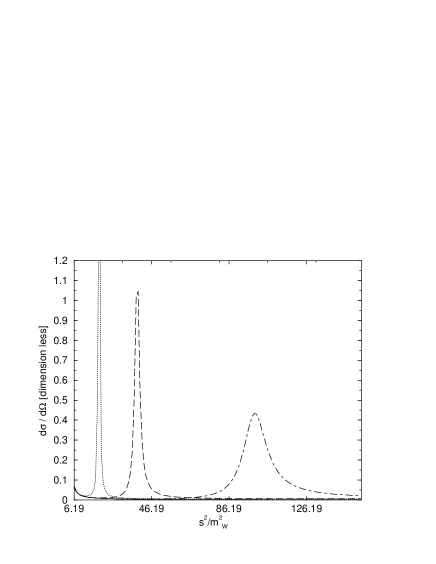
Figure 8: Dimensionless cross section of the reaction $W_{L}^{+}W_{L}^{-}\to W_{L}^{+}+W_{L}^{-}$ including the $H^{*}$ boson. The solid line is the standard model cross section, the dotted line corresponds to a $H^{*}$ boson of mass 350 GeV, with $\Gamma=6.72$ GeV and $\bar{g}_{H^{*}}=0.8g$, the long dashed line to a $H^{*}$ boson of mass 500 GeV, with $\Gamma=17.6$ GeV and $\bar{g}_{H^{*}}=0.7g$ and the dot-dashed line to a $W^{3*}$ boson of mass 800 GeV, with $\Gamma=58.25$ GeV and $\bar{g}_{H^{*}}=0.6g$.

Figure 9: Ratio of the cross-section for the of the reaction involving the $d$-wave to the standard model cross-section for different values of the $d$-wave mass and different coupling constant. The dotted line corresponds to a d-wave of mass 350 GeV, with $\Gamma=4.38$ GeV and $\bar{g}_{W^{3*}}=0.8g$, the long dashed line to a d-wave of mass 500 GeV, with $\Gamma=27.49$ GeV and $\bar{g}_{W^{3*}}=0.7g$ and the dot-dashed line to a d-wave of mass 800 GeV, with $\Gamma=251.03$ GeV and $\bar{g}_{W^{3*}}=0.6g$.

5 Conclusions

We have discussed the production of a neutral $d$-wave $D^{3}$ at the LHC or at a linear collider. If the mass of this particle is of the order of the scale of the theory, i.e. 300 GeV, it can be produced at these colliders. We have also shown that this particle as well as radial excitations of the Higgs boson and $Z$ boson would spoil the cancellation of the leading powers in $s$ of in the reaction $W^{+}_{L}+W^{-}_{L}\to W^{+}_{L}+W^{-}_{L}$, thus any new particle contributing to that reaction will have a large impact already at energies well below the mass of this new particle. This reaction is thus not only of prime interest if the Higgs boson is heavy but should also be studied if the Higgs boson was light.

References

• [1] X. Calmet and H. Fritzsch, Phys. Lett. B496, 161 (2000) [hep-ph/0008243].
• [2] G. ’t Hooft, in “Erice 1998, From the Planck length to the Hubble radius” 216-236, hep-th/9812204, see also G. ’t Hooft, in “Recent Developments In Gauge Theories”, Cargesè 1979, ed. G. ’t Hooft et al. Plenum Press, New York, 1980, Lecture II, p.117.
• [3] X. Calmet and H. Fritzsch, Phys. Lett. B496, 190 (2000) [hep-ph/0008252].
• [4] S. L. Glashow, Nucl. Phys. 22, 579 (1961), S. Weinberg, Phys. Rev. Lett. 19, 1264 (1967).
• [5] P. Chiappetta, J. L. Kneur, S. Larbi and S. Narison, Phys. Lett. B 193, 346 (1987), J. L. Kneur, S. Larbi and S. Narison, Phys. Lett. B 194, 147 (1987).
• [6] H. van Dam and M. Veltman, Nucl. Phys. B22, 397 (1970), V. I. Zakharov, JETP Lett. 12, 312 (1970).
• [7] J. F. Donoghue, E. Golowich and B. R. Holstein, Dynamics of the standard model, Cambridge, UK: Univ. Pr. (1992) 540 p.
• [8] D. A. Dicus and V. S. Mathur, Phys. Rev. D 7 (1973) 3111, M. Veltman, Acta Phys. Polon. B8, 475 (1977), see also M. S. Chanowitz and M. K. Gaillard, Phys. Lett. B142, 85 (1984), M. S. Chanowitz and M. K. Gaillard, Nucl. Phys. B261, 379 (1985).
• [9] M. J. Duncan, G. L. Kane and W. W. Repko, Nucl. Phys. B272, 517 (1986).
• [10] A. Denner and T. Hahn, Nucl. Phys. B525, 27 (1998) [hep-ph/9711302].
• [11] J. F. Gunion, H. E. Haber, G. L. Kane and S. Dawson, “The Higgs Hunter’s Guide”, SCIPP-89/13.
• [12] C. H. Llewellyn Smith, Phys. Lett.  B46 233 (1973), J. M. Cornwall, D. N. Levin and G. Tiktopoulos, Phys. Rev. Lett.  30 1268 (1973), J. M. Cornwall, D. N. Levin and G. Tiktopoulos, Phys. Rev.  D10 1145 (1974).