General Flavor Blind MSSM and CP Violation

Abstract

We study the implications on flavor changing neutral current and $CP$ violating processes in the context of supersymmetric theories without a new flavor structure (flavor blind supersymmetry). The low energy parameters are determined by the running of the soft breaking terms from the grand unified scale with SUSY phases consistent with the EDM constraints. We find that the $CP$ asymmetry in $b\to s\gamma$ can reach large values potentially measurable at B factories, especially in the low $BR(b\to s\gamma)$ region. We perform a fit of the unitarity triangle including all the relevant observables. In this case, no sizeable deviations from the SM expectations are found. Finally we analyze the SUSY contributions to the anomalous magnetic moment of the muon pointing out its impact on the $b\to s\gamma$ $CP$ asymmetry and on the SUSY spectrum including chargino and stop masses.

I Introduction

The Standard Model (SM) of electroweak and strong interactions has been extremely successful in the description of all known high energy phenomena up to energies of $\mathcal{O}(100\ \mbox{GeV})$. Still, this impressive theoretical construction is not complete if only because it does not account for gravitational interactions. Moreover, several theoretical questions remain unanswered and some cosmological observations can not be properly accommodated.

From the point of view of theory, the SM includes three independent gauge coupling constants that in a more complete framework would be expected to emerge from a single unified parameter. In turn, this requirement causes the so–called gauge hierarchy problem: scalar masses are not protected by any symmetry against radiative corrections that tend to be of the order of the highest scale present in the theory. In a grand unified scenario, this scale is usually close to the Plank scale; therefore, a great amount of fine tuning is necessary to keep the Higgs mass close to the electroweak scale. Furthermore, in the SM picture, several cosmological observations seem difficult to account for. In first place, a suitable candidate to reproduce the required dark matter content of the universe is not provided; moreover, the tiny $CP$ violation present in the Cabibbo–Kobayashi–Maskawa (CKM) matrix does not succeed to generate the necessary baryon–antibaryon asymmetry. Finally in the SM framework is not possible to include an inflationary stage at the early universe.

Low energy supersymmetry (SUSY) is the most promising extension of the SM where all these problems can be successfully solved. Indeed it stabilizes the gauge hierarchies and successfully unifies the gauge couplings with remarkably high accuracy. It includes many possible dark matter candidates and it can naturally account for inflation as well. Moreover, the many additional phases present in any SUSY model can generate the required baryon asymmetry. Not to mention that any fundamental theory including gravity almost necessarily contains SUSY as well (although the scale of SUSY breaking is not forced to be of the order of the electroweak scale).

For all these reasons, SUSY is one of the most attractive theories beyond the SM. The so–called Minimal Supersymmetric SM (MSSM) is obtained adding to the SM spectrum the smallest number of new fields consistent with SUSY. This recipe does not unambiguously define a single supersymmetric theory. In fact, to specify completely the theory, it is necessary to fix the soft breaking terms: this amounts to 124 parameters at the electroweak scale (luckily enough, most of this enormous parameter space is already ruled out by phenomenological constraints).

In this paper, we focus on a certain class of SUSY extensions that we call flavor blind MSSM. With this term we refer to a model where the soft breaking terms at the grand unification (GUT) scale do not introduce any new flavor structure beyond the usual Yukawa matrices. These matrices are already present in the superpotential and are necessary to reproduce correctly the fermion masses and mixing angles. In this restricted class of models, the number of parameters is largely reduced and it is therefore possible to perform a complete phenomenological analysis. Indeed, many features of such models are shared by most MSSMs. In particular the spectrum and the flavor conserving processes are not expected to be strongly influenced by extra flavor structures.

The experimental search for SUSY proceeds through two main lines. The main path to establish the existence of low energy SUSY is the direct search of SUSY particles at present and future colliders with high enough energy. In addition to these direct searches it is necessary to perform also the so–called “indirect searches” of SUSY particles by measuring suitable observables with high precision at lower energies. Virtual SUSY particle contributions appear in the quantum corrections to characteristic observables and may be traced out if the experimental and theoretical precisions are sufficient. These indirect searches of SUSY is particularly important as long as the collider energies are not, presently, high enough to directly produce the SUSY particles.

There are two prominent classes of observables which are especially well suited for probing virtual SUSY particles. These are observables sensitive to $CP$ violation and observables involving flavor changing neutral currents (FCNC). In the context of indirect SUSY searches, the most interesting $CP$ violating observables are those where the SM predictions turn out to be very small. Similarly, the study of FCNC within SUSY is motivated by the absence of SM tree level contributions; therefore, one–loop SUSY contributions may be large enough to give sizeable deviations.

The electric dipole moments (EDMs) of electron and neutron are well–known examples of flavor conserving observables sensitive to $CP$ violation. The SM predictions for these quantities are extremely small, because the first nonvanishing contributions arise at higher–loop level. These predictions are several orders of magnitude below the experimental limits. The SUSY contributions arise already at one–loop level and can be close to the experimental upper bounds. Therefore, the electron and neutron EDMs are well suited to yield important information about SUSY models and can considerably restrict the allowed parameter regions. However, in the calculation of the electron and neutron EDMs it turns out that large cancellations between the different SUSY contributions can occur. This peculiarity has to be taken into account when deriving bounds on the SUSY parameters and phases in specific models. The allowed SUSY parameter space, especially the phases, can be much larger due to these cancellations.

An important example of an observable involving FCNC is the branching ratio of the rare $b$–quark decay $b\rightarrow s\gamma$. The SM prediction at one–loop level for the branching ratio is comparable in size with the experimentally measured value. Therefore, a comparison of the theoretical predictions with the experimental value leads to considerable restrictions on the parameter space of SUSY models.

In the present paper we study in a systematic way the restrictions on the SUSY parameters and complex phases which can be derived from the experimental information on FCNC and on $CP$ violation. The electron EDM and the branching ratio of the rare decay $b\rightarrow s\gamma$ constitute the two most severe constraints. We define the SUSY model at the GUT scale and determine the soft SUSY breaking parameters at the weak scale by evolving them down with the renormalization group equations (RGE). We fix $|\mu|^{2}$ by demanding radiative breaking of the electroweak $SU(2)_{L}\times U(1)$ symmetry. At this scale we impose the constraints from direct searches and from the $\rho$–parameter, as well as the requirements of color and electric charge conservation and the lightest SUSY particle (LSP) to be neutral. With these sets of soft SUSY parameters we calculate the EDM of the electron and the branching ratio of $b\rightarrow s\gamma$ and compare them with the experimental data. The sets in agreement with the experimental constraints are used to calculate the $CP$ asymmetry of $b\rightarrow s\gamma$ and the SUSY contributions to the $CP$-violating quantities $\epsilon_{K}$, $\Delta M_{B_{d}}$ and $\Delta M_{B_{s}}$. With these results we study the modifications of the so–called unitarity triangle. Finally we calculate the SUSY contributions to the muon anomalous magnetic moment in order to quantify the effect of the recent experimental data on the observables we are interested in.

II GUT–inspired MSSM spectrum at $M_{W}$

In the flavor blind MSSM the most general structure of the soft breaking parameters at the GUT scale is

$$(M_{Q}^{2})_{ij}=M_{Q}^{2}\ \delta_{ij},\ \ \ (M_{U}^{2})_{ij}=M_{U}^{2}\ \delta_{ij},\ \ \ (M_{D}^{2})_{ij}=M_{D}^{2}\ \delta_{ij},$$ (1)

$$(M_{L}^{2})_{ij}=M_{L}^{2}\ \delta_{ij},\ \ \ (M_{E}^{2})_{ij}=M_{E}^{2}\ \delta_{ij},\ \ \ \ \ M_{H_{1}}^{2},\ \ \ \ \ \ M_{H_{2}}^{2},\ \ \$$ (2)

$$(Y^{A}_{U})_{ij}=A_{U}e^{i\phi_{A_{U}}}(Y_{U})_{ij},\ \ \ (Y^{A}_{D})_{ij}=A_{D}e^{i\phi_{A_{D}}}(Y_{D})_{ij},$$ (3)

$$(Y^{A}_{E})_{ij}=A_{E}e^{i\phi_{A_{E}}}(Y_{E})_{ij},$$ (4)

where $i,j$ are family indices, the $Y^{A}_{f}$ are trilinear scalar couplings and $Y_{f}$ denote the Yukawa matrices. All the allowed phases are explicitly written, with the only exception of possible phases in the Yukawa matrices. In addition, we have a universal gaugino mass parameter $M_{1/2}$ that we can take as real while the $\mu$ parameter in the superpotential is complex. Notice that $M_{H_{1}}$ and $M_{H_{2}}$ are only the Higgs soft breaking masses and not the complete Higgs masses that can be computed from the scalar potential.

As the number of parameters in Eq. (2.1) is still rather large, for our present study we will make further simplifying assumptions. The first case we consider is the simplest version of the constrained MSSM, where we take the following independent parameters:

  (I)

$M_{1/2}$, $M_{0}^{2}$, $|A_{0}|$, $\tan\beta$, $\phi_{\mu}$, $\phi_{A_{0}}$,

which means that we impose $M_{Q}^{2}=M_{U}^{2}=M_{D}^{2}=M_{L}^{2}=M_{E}^{2}=M^{2}_{H_{1}}=M^{2}_{H_{2}}=M_{0}^{2}$, $A_{U}=A_{D}=A_{E}=A_{0}$ and $\phi_{A_{U}}=\phi_{A_{D}}=\phi_{A_{E}}=\phi_{A_{0}}$.

The second case refers to the SUSY $SU(5)$ model. In this model the sfermions are in a $\bar{5}$ and a $10$ multiplet and the Higgs doublets are members of different $5$ multiplets. We take the following set of parameters:

  (II)

$M_{1/2}$, $M_{5}^{2}$, $M_{10}^{2}$, $M_{H_{1}}^{2}$, $M_{H_{2}}^{2}$, $|A_{u}|$, $|A_{d}|$, $\tan\beta$, $\phi_{\mu}$, $\phi_{A_{u}}$, $\phi_{A_{d}}$,

where now we have $M_{D}^{2}=M_{L}^{2}=M_{5}^{2}$, $M_{Q}^{2}=M_{U}^{2}=M_{E}^{2}=M_{10}^{2}$, $A_{U}=A_{u}$, $A_{D}=A_{E}=A_{d}$ and $\phi_{A_{U}}=\phi_{A_{u}}$, $\phi_{A_{D}}=\phi_{A_{E}}=\phi_{A_{d}}$.

Although the number of parameters in set (II) is significantly larger than in set (I), the problem can be handled and a full RGE evolution and an analysis of the low–energy SUSY spectrum is possible. In our analysis, we have used two–loop RGEs as given in [1] and one–loop masses as given in [2].

In the following, we are going to discuss the main features of the low–energy spectrum relevant for $CP$ violating and FCNC observables. In particular we are interested in electric dipole moments (EDM), $\varepsilon_{K}$, $\Delta M_{B_{d}}$, $\Delta M_{B_{s}}$, $BR(b\to s\gamma)$ and the anomalous magnetic moment of the muon ($a_{\mu^{+}}$).

The dominant contributions in flavor conserving observables are mediated by chargino–sneutrino diagrams for the electron EDM and for $a_{\mu^{+}}$ and by both chargino–squark and gluino–squark diagrams for the neutron EDM. Since we are interested in a light SUSY spectrum, we will also consider sub–dominant neutralino–sfermion contributions which are important in a part of the parameter space where cancellations can occur [3, 4]. The main contributions for flavor changing $CP$ violating observables ($\varepsilon_{K}$, $\Delta M_{B_{d}}$, $\Delta M_{B_{s}}$, $BR(b\to s\gamma)$) are given by up squark–chargino, top–charged Higgs and the usual SM $W$–boson contributions. Hence, we are interested in the following part of the low energy spectrum: $\chi^{+}$, $\chi^{0}$, $\tilde{g}$, $H^{+}$, $\tilde{t}$, light $\tilde{q}$ and $\tilde{l}$.

A very good approximation for their masses in terms of the initial parameters is already given by the solution of the one–loop RGEs [5, 6, 7]. In tables I, II, III, IV, and V, we present the numerical solution of these equations for the various parameters entering the mass formulae for different values of $\tan\beta$.

A further important parameter entering the mass matrices is $\mu$. We calculate its modulus from the requirement of electroweak symmetry breaking, using the complete one–loop corrections for all particles [2]. To get an understanding of the general behavior, we use the corresponding tree level formula which reads:

$$|\mu|^{2} = \frac{m^{2}_{H_{2}}\sin^{2}\beta-m^{2}_{H_{1}}\cos^{2}\beta}{\cos 2\beta}-\frac{m^{2}_{Z}}{2}\ ,$$ (5)

where we write in lower cases the physical masses at the electroweak scale. It is well known that the tree level result can be modified by large one–loop corrections that are taken into account in our numerical computations.

In first place, we consider the charged Higgs mass which is connected at tree level with the $\mu$ parameter by:

$$m^{2}_{H^{+}} = m^{2}_{A^{0}}+m^{2}_{W}=m^{2}_{H_{2}}+m^{2}_{H_{1}}+2|\mu|^{2}+m^{2}_{W}$$ (6)

$$= \frac{\tan^{2}\beta+1}{\tan^{2}\beta-1}(m^{2}_{H_{1}}-m^{2}_{H_{2}})+m^{2}_{W}-m^{2}_{Z}$$ (7)

Eq. (6) implies that the “tree level” $\tan\beta$ dependence of $m^{2}_{H^{+}}$ is always small, and for $\tan\beta\geq 3$ the only important dependence comes through the $m_{H_{1}}^{2}$ and $m_{H_{2}}^{2}$ parameters. Inserting the numbers given Table I we obtain the result displayed in Table II for the CMSSM case and in Table III for $SU(5)$.

Let us first discuss the CMSSM case: It is clear from Table II that the main contribution stems from the gaugino mass, $M_{1/2}^{2}$, both for $|\mu|^{2}$ and $m_{H^{+}}^{2}$. Other relevant contributions come from the universal scalar mass $M_{0}^{2}$ and the $A_{0}$–$M_{1/2}$ interference term. In this framework, the size of the coefficient $c_{2}$ implies that within CMSSM $|\mu|$ is, in general, larger than $M_{2}\simeq 0.81M_{1/2}$. The only possible exception to this rule could come from the negative sign of the $c_{3}$ coefficient for the $A_{0}$–$M_{1/2}$ interference. Only with large $\tan\beta$ and a value of $A_{0}\geq 5.5M_{1/2}$ it would be possible to change the above situation. However, this possibility is ruled out as soon as we take into account the direct constraints on gaugino and scalar masses and specially the requirement of the absence of charge and color breaking minima which forbids large values of $A_{0}$ [8]. This fact has important consequences, in particular it implies that in the CMSSM the lightest chargino, as well as the lighter two neutralinos, will be gaugino–like. The behavior of $m_{H^{+}}^{2}$ is similar to $|\mu|^{2}$, although the contribution from the $M_{0}^{2}$ coefficient $c_{1}$ is now more important. Finally, it is obvious from the tables that with increasing $\tan\beta$, both $|\mu|$ and $m_{H^{+}}$ decrease. In the $SU(5)$ scenario we have different scalar masses for the two Higgs doublets and the particles in different multiplets, as well as different trilinear terms. The physical masses at the electroweak scale depend, in this case, on the values of these parameters at $M_{GUT}$. In Table III we see the dependence of $m_{H^{+}}$ on these initial values. We must emphasize that this is only a decomposition of the coefficients in Table II in different contributions. Therefore, the sum of the coefficients $c_{1}$, $c_{2}$, $c_{3}$ and $c_{4}$ in Table III corresponds to the coefficient $c_{1}$ in Table II and so on. In this decomposition, it is interesting to notice the negative sign of the coefficient $c_{4}$. This means that with a sufficiently large initial value for $M^{2}_{H_{2}}$ and a moderate value of $M_{1/2}$ it is possible to have $|\mu|\leq M_{2}$ and a large higgsino component in the lightest chargino and neutralinos; it is so possible to overcome the bounds that forbid this possibility in the CMSSM case.

We now present the numerical results obtained using the RGEs at the two loop level. In Fig. 1 we show the scatter plot of the mass of the charged Higgs boson versus $\tan\beta$ for the CMSSM and the SU(5) cases. In this and all the following scatter plots we vary the scalar and gaugino masses at $M_{GUT}$ in the range $100\ \mbox{GeV}<M_{i}<1\ \mbox{TeV}$, the trilinear terms $0<|A_{d}|^{2}<M^{2}_{10}+M^{2}_{5}+M^{2}_{H_{1}}$, $0<|A_{u}|^{2}<2\,M^{2}_{10}+M^{2}_{H_{2}}$ while their phases are arbitrary. Finally we take $4<\tan\beta<50$, where the lower bound takes into account the limits on the lightest neutral Higgs mass. Moreover, we apply the following set of constraints:

• Absence of charge and color breaking minima and directions unbounded from below [8].

• Lower bounds on masses from direct searches [9], in particular $m_{\chi^{+}_{i}}>90\ \mbox{GeV}$, $m_{\tilde{t}_{i}}>90\ \mbox{GeV}$, $m_{\chi^{0}}>33\ \mbox{GeV}$ and $m_{\tilde{\nu}}>33\ \mbox{GeV}$.

• The acceptable range in the $b\to s\gamma$ branching ratio is between $2\times 10^{-4}$ and $4.5\times 10^{-4}$[10].

• The lightest supersymmetric particle is neutral.

• The upper bound on the electron EDM is $|d^{e}|\leq 4.0\times 10^{-27}\ e\ \mbox{cm}$.

In any $R$-parity conserving MSSM, a further constraint would be the relic density of the lightest supersymmetric particle, $\Omega_{\chi}h^{2}\leq 0.4$. However, we have not included it because a careful treatment of this constraint, in the presence of non–vanishing phases, is beyond the scope of this paper.

In Fig. 1, the black dots fulfill the $b\to s\gamma$ constraint, whereas in the case of the bright open circles this constraint is violated. The most relevant feature of these plots is the heavy mass of the charged Higgs in most of the parameter space, $m_{H^{+}}\raise 1.29167pt\hbox{$\;>$\kern-7.5pt\raise-4.73611pt\hbox{$\sim\;$}}400\ \mbox{GeV}$. In the CMSSM case, we see that $m_{H^{+}}\geq 400\ \mbox{GeV}$ except for a few exceptions at intermediate $\tan\beta$. This is due to the decrease of the $c_{2}$ coefficient with increasing $\tan\beta$; in this region the $b\to s\gamma$ constraint is very important too. At small $\tan\beta$, the chargino contributions cannot usually compete with the charged Higgs ones and hence the same bound as in two–Higgs doublet models applies, i.e. $m_{H^{+}}>250\ \mbox{GeV}$ [11]. With moderate or large values of $\tan\beta$, the chargino contribution can partially cancel the charged Higgs contribution and hence lower values are allowed [12]. At larger $\tan\beta$ values, this cancellation is no longer possible and the $b\to s\gamma$ constraint turns out to be more effective for low SUSY masses.

In the $SU(5)$ case, a similar situation occurs although more cancellations are possible because now the charged Higgs and sfermion masses are independent at the GUT scale.

Beside the charginos and the charged Higgs, that we discussed above, the stops are particularly interesting in the processes we consider. Neglecting for the moment the so–called D–terms, one gets for the masses:

$$m^{2}_{{\tilde{t}}_{1,2}} = \frac{1}{2}\left(m^{2}_{Q_{3}}+m^{2}_{U_{3}}+2m^{2}_{t}\mp\sqrt{(m^{2}_{Q_{3}}-m^{2}_{U_{3}})^{2}+4m_{t}^{2}|A_{t}^{*}-\mu\cot\beta|^{2}}\right).$$ (8)

Fig. 2 shows a scatter plot of the lightest chargino versus the lightest stop masses. It is very interesting to notice the very strong correlation among these masses. In fact, in the CMSSM, $|\mu|\simeq\sqrt{3}M_{1/2}$ is always larger than $M_{2}\simeq 0.8M_{1/2}$ and the lightest chargino, whose mass is bounded by direct searches to be heavier than $90\ \mbox{GeV}$, is approximately a gaugino. On the other side, we see in Table I that the lightest stop will always be dominantly right–handed. Writing Eq. (8) as a function of the high scale parameters in the CMSSM case we find:

$$m^{2}_{{\tilde{t}}_{1,2}} = 0.43M^{2}_{0}+4.55M^{2}_{1/2}+m^{2}_{t}+0.19M_{1/2}\mbox{Re}(A_{0})$$ (10)

$$\mp\frac{\displaystyle{1}}{\displaystyle{2}}M_{1/2}\sqrt{2.25M^{2}_{1/2}+1.13\,M^{2}_{0}+20.2\,m^{2}_{t}}$$

where a slight dependence on $\tan\beta$ of the coefficients is neglected. Using $m_{\chi^{+}_{1}}\simeq M_{2}\simeq 0.81M_{1/2}$, we further get

$$m^{2}_{{\tilde{t}}_{1,2}} = 0.43M^{2}_{0}+6.93m^{2}_{\chi^{+}_{1}}+m^{2}_{t}+0.23m_{\chi^{+}_{1}}\mbox{Re}(A_{0})$$ (12)

$$\mp\frac{\displaystyle{1}}{\displaystyle{2}}m_{\chi^{+}_{1}}\sqrt{5.23m^{2}_{\chi^{+}_{1}}+1.72\,M^{2}_{0}+30.8\,m^{2}_{t}}\ .$$

For the mixing the following approximate result can be derived:

$$|\tan 2\theta_{\tilde{t}}|\simeq\frac{2m_{t}|0.2A_{0}-(2-\sqrt{3}\cot\beta\,\,e^{-i\phi_{\mu}})M_{1/2}|}{|0.37M^{2}_{0}+1.3M^{2}_{1/2}-0.13M_{1/2}\mbox{Re}(A^{0})|}$$ (13)

In case that $A_{0}\simeq M_{1/2}\simeq M_{0}\simeq m_{t}$ and moderate/large $\tan\beta$ one finds that $|\theta_{\tilde{t}}|\simeq 1.0$. Therefore, the lighter stop is clearly more “right handed” than the heavier one. Note that for larger $M_{1/2}$ and/or $M_{0}$ the mixing angle grows and, thus, the ’right–handed’ component of the lighter top squark increases. An analogue formula can be found for the phase:

$$\tan\phi_{\tilde{t}}\simeq\frac{0.2\,\mbox{Im}(A_{0})-\sqrt{3}\cot\beta\sin\phi_{\mu}M_{1/2}}{0.2\,\mbox{Re}(A_{0})-(2-\sqrt{3}\cot\beta\cos\phi_{\mu})M_{1/2}}$$ (14)

It is obvious from this formula that the $CP$ phase of the top squark is relatively small at the electroweak scale even if it is maximal at the GUT scale. This is a result of the fix–point structure which governs the corresponding RGEs.

From Eq. (12), for $100\ \mbox{GeV}<M_{0}<1\ \mbox{TeV}$ and with $m_{\chi^{+}_{1}}=100\ \mbox{GeV}$ we get an allowed range for the stop mass $240\ \mbox{GeV}\raise 1.29167pt\hbox{$\;<$\kern-7.5pt\raise-4.73611pt\hbox{$\sim\;$}}m_{\tilde{t}_{1}}\raise 1.29167pt\hbox{$\;<$\kern-7.5pt\raise-4.73611pt\hbox{$\sim\;$}}660\ \mbox{GeV}$. As we can see from the plot the correlation between the two masses is maintained for larger chargino masses. The “splitting” into two bands is due to the fact that the phase of $\mu$ is rather small and, thus, it is concentrated around $0$ and $\pi$. One band is more populated than the other because, according to the EDM constraint, there is a preferred phase difference between $A_{0}$ and $\mu$. In the case of $SU(5)$, the main difference is that the Higgs masses are not tied to the other scalar masses and now may be quite different. This has important effects in the radiative symmetry breaking; in fact, lower values of $\mu$ are possible and the lightest chargino can have a dominant higgsino part. In scenarios where $|\mu|\raise 1.29167pt\hbox{$\;<$\kern-7.5pt\raise-4.73611pt\hbox{$\sim\;$}}M_{2}$ we find that the stop masses are somewhat lower compared to the CMSSM case because of the requirement that $M^{2}_{H_{2}}>>M^{2}_{10}$ and of the negative sign of the $c_{i4}$ coefficient in Table I for the $m_{Q_{3}}$ and $m_{U_{3}}$ parameters. In the plot we see that this effect tends to slightly soften the stop–chargino correlation, however, if we plot $m_{\tilde{t_{1}}}$ versus $M_{2}$ much of this correlation is again recovered. Moreover the up–type squarks can have a different $A$–parameter value compared to the down–type squarks and the charged leptons. This leads to a stronger overlap of the two bands. We must emphasize here that, due to gluino dominance in the soft–term evolution, this kind of correlation is general in any RGE evolved MSSM from some GUT initial conditions assuming that also gaugino masses unify. In summary, this implies that the “light stop and chargino” scenario [13, 14, 15, 16] must be shifted to stop masses in the range of $250\ \mbox{GeV}$ for chargino masses of $100\ \mbox{GeV}$. As we will see in the next section this has very important consequences for the searches of low energy FCNC and $CP$ violating effects.

Analogously, a very similar correlation can be obtained for all the other squarks and Higgs bosons, although it is not as stringent as in the stop–chargino case. We roughly get,

$$m_{\tilde{q}}^{2}\simeq 9.3\times m_{\chi^{+}_{1}}^{2}+M_{0}^{2}.$$ (15)

It is an interesting fact that the allowed bands are always wider that in the case of the lighter stop due to the larger coefficient of $M_{0}^{2}$ and are always above the band plotted in Fig. 2.

III Low energy observables

Indirect searches in $CP$ violation and FCNC experiments play a very important role in the race for the discovery of SUSY. In these rare processes, SM contributions are small and hence supersymmetry is allowed to compete on equal ground. We are mainly interested in $CP$ violation experiments, since new results are coming from $B$–factories. With this goal, the first observables we must analyze are the electric dipole moments (EDM) of the quarks and leptons since they provide the most stringent constraints on the new supersymmetric phases. In this paper, we concentrate on the electron EDM because the constraint it provides is already very tight and its theoretical computation is independent of hadronic uncertainties that plague the neutron EDM calculation. Then, with the information obtained from the previous analysis of the MSSM spectrum, we address the study of the main $CP$ violating and FCNC observables consistent with this EDM constraint. In first place, we study the $CP$ violation asymmetry in the $b\to s\gamma$ decay which, apart from EDMs, is an especially sensitive observable to the new SUSY phases. Then, we make a full analysis of the unitarity triangle which includes the study of $\varepsilon_{K}$, $\Delta M_{B_{d}}$ and $\Delta M_{B_{s}}$ as well as the determination of the angles through the $CP$ asymmetries. Finally, we complete our discussion with a study of the anomalous magnetic moment of the muon, whose measurement has been recently updated at BNL [17].

A EDMs

The EDM of a spin–$\frac{1}{2}$ particle is the coefficient, $d^{f}$, of the effective operator,

$${\mathcal{L}}_{E}=-(i/2)d^{f}\bar{f}\gamma^{5}\sigma_{\mu\nu}fF^{\mu\nu}\enspace.$$ (16)

This $CP$ violating vertex is absent at tree level both in the SM and in SUSY. It is generated in the SM as a three loop effect [18], whereas SUSY contributions arise generically as one loop effects. Thus, these contributions are naturally expected to be much bigger than the stringent limits obtained in various EDM experiments, namely the neutron [19, 20], the Mercury atom [21], and the Thallium atom [22] EDMs, the latter being mostly sensitive to the EDM of the electron. So far, a fully accepted explanation for the smallness of the EDMs in SUSY is missing and this fact gives rise to the most severe part of the so–called supersymmetric $CP$ problem.

It is well–known, since the beginning of the SUSY phenomenology era, that the effects of $\phi_{A}$ and $\phi_{\mu}$ on the electric and chromoelectric dipole moments of the light quarks imply that $\phi_{A,\mu}$ should be $<10^{-2}$ [23], unless one pushes SUSY masses up to ${\mathcal{O}}$($1\ \mbox{TeV}$). This strong constraint led most of the authors dealing with the MSSM afterwards to simply set $\phi_{A}$ and $\phi_{\mu}$ exactly equal to zero. However, in recent years, the attitude towards the EDM problem in SUSY and the consequent suppression of the SUSY phases has significantly changed. Indeed, options have been envisaged allowing for a conveniently suppressed SUSY contribution to the EDM even in the presence of large (sometimes maximal) SUSY phases. Methods of suppressing the EDMs consist in the cancellation of various SUSY contributions among themselves [3, 4], approximately degenerate heavy sfermions for the first two generations [24, 25, 26] and non–universality of the soft breaking parameters at the unification scale [28, 29].

In our flavor blind scenario, the latter possibility is obviously not present, and as discussed in the previous section, the SUSY spectrum is fixed by RGE evolution in terms of the initial conditions at $M_{GUT}$. We have seen that the first two generations are always naturally heavier than the third one and hence the second mechanism can be considered in some regions of the parameter space [30]. Still, in a pure MSSM scenario with a SUSY spectrum below the TeV scale, a cancellation between different contributions is the main mechanism that can allow large SUSY phases.

In the following, we calculate explicitly the electron EDM and apply the experimental limits to this value. As shown in [3, 4], there exist regions of the parameter space where sizeable phases are still allowed. We mainly concentrate on these regions using the electron EDM to obtain the allowed phases after RGE evolution. We pick the electron EDM for this procedure because, on the theoretical side, its calculation is simple and well under control. Chargino and neutralino loops are the only SUSY contributions:

$$d^{e}=d^{e}_{\tilde{\chi}^{+}}+d^{e}_{\tilde{\chi}^{0}}\enspace.$$ (17)

The supersymmetric contributions to the EDMs of leptons and quarks have been calculated in various papers (see [3, 4, 23] and references therein). We use the formulae and numerical results as given in [4]. The chargino contribution to the electron EDM can be brought to the very simple form:

$$\frac{1}{e}d^{e}_{\tilde{\chi}^{+}} = \frac{\alpha_{em}m_{e}\tan\beta\,\mathrm{Im}\,[M_{2}\mu]}{4\pi\sin^{2}\theta_{W}(m_{\tilde{\chi}^{+}_{2}}^{2}-m_{\tilde{\chi}^{+}_{1}}^{2})}\times\frac{1}{m_{\tilde{\nu}_{e}}^{2}}\left(F_{3}(r_{1})-F_{3}(r_{2})\right)$$ (18)

where $r_{i}=m_{\tilde{\chi}^{+}_{i}}^{2}/m_{\tilde{\nu}_{e}}^{2}$ and the loop function $F_{3}(r_{i})$ can be found in the appendix.

The neutralino contribution to the electron EDM involves complex neutralino and sfermion mixings. Hence, its expression is not especially simple [4]:

$$\frac{1}{e}d^{f}_{\tilde{\chi}^{0}}=-\frac{Q_{f}}{8\pi}\frac{\alpha}{\sin^{2}\theta_{W}}\sum_{k=1}^{4}\sum_{m=1}^{2}\eta^{f}_{mk}\times\frac{m_{\tilde{\chi}^{0}_{k}}}{m^{2}_{\tilde{f}_{m}}}F_{4}(\frac{m^{2}_{\tilde{\chi}^{0}_{k}}}{m^{2}_{\tilde{f}_{m}}})$$ (19)

where

$$\eta^{f}_{mk} = (-1)^{m}\sin 2\theta_{\tilde{f}}\,\mathrm{Im}\,[((h^{f}_{Lk})^{2}-f^{f}_{Lk}f^{f*}_{Rk})e^{-i\varphi_{\tilde{f}}}]$$ (22)

$$-(1-(-1)^{m}\cos 2\theta_{\tilde{f}})\,\mathrm{Im}\,[h^{f}_{Lk}f^{f*}_{Lk}]$$

$$-(1+(-1)^{m}\cos 2\theta_{\tilde{f}})\,\mathrm{Im}\,[h^{f}_{Lk}f^{f}_{Rk}]\enspace,$$

in terms of the neutralino–sfermion couplings,

$$h^{e}_{Lj} = -Y_{e}(\cos\beta N_{3j}+\sin\beta N_{4j})\enspace,$$ (24)

$$h^{e}_{Rj} = -Y_{e}(\cos\beta N^{*}_{3j}+\sin\beta N^{*}_{4j})=h^{e\,*}_{Lj},$$ (25)

$$f^{f}_{Lj} = -\left[Q_{f}\sin 2\theta_{W}N^{*}_{1j}+(1-2Q_{f}\sin^{2}\theta_{W})N^{*}_{2j}\right]/(\sqrt{2}\cos\theta_{W})\enspace,$$ (26)

$$f^{f}_{Rj} = \left[Q_{f}\sin 2\theta_{W}N_{1j}+(-2Q_{f}\sin^{2}\theta_{W})N_{2j}\right]/(\sqrt{2}\cos\theta_{W})\enspace.$$ (27)

with $Y_{e}=m_{e}/(\sqrt{2}\,m_{W}\cos\beta)$ and the definitions for the neutralino mixing matrix $N_{\alpha j}$ and the selectron mixing angle $\theta_{\tilde{f}}$ and phase $\varphi_{\tilde{f}}$ as well as the loop function $F_{4}$ can be found in the Appendices.

With the help of Eqs. (18) and (19) we can readily calculate the electron EDM. If both contributions are separately required to satisfy the experimental bound, $(1.8\pm 1.2\pm 1.0)\times 10^{-27}\mbox{$e$ cm}$, we obtain, from the electron EDM constraint, $\phi_{\mu}\raise 1.29167pt\hbox{$\;<$\kern-7.5pt\raise-4.73611pt\hbox{$\sim\;$}}0.01$ and $\phi_{A}\raise 1.29167pt\hbox{$\;<$\kern-7.5pt\raise-4.73611pt\hbox{$\sim\;$}}0.3$ for sfermion and gaugino masses of $100\ \mbox{GeV}$ at $M_{GUT}$. Notice that the constraint on $\phi_{A}$ is always less stringent than the one on $\phi_{\mu}$ because the latter contributes also through chargino mixing and it is enhanced by a $\tan\beta$ factor in the down squarks and charged sleptons mass matrices.

However, if both contributions are considered simultaneously, a negative interference occurs in particular regions of the parameter space and larger phases are allowed under these special conditions. In Fig. 3 we show the allowed regions for $\phi_{\mu}$ and $\phi_{A_{e}}$ as specified at $M_{GUT}$, and the correlation of $\phi_{\mu}$ with the scalar mass, $M_{0}$. As we can see in these figures, it is possible to find any value for $\phi_{A_{e}}$ although there is a correlation with the value of $\phi_{\mu}$. The value of $\phi_{\mu}$ itself is much more constrained; however, values up to $\phi_{\mu}=0.4$ are still allowed, especially for regions of relatively large masses. This may appear surprising, given that the usual values quoted from EDM cancellations are $\phi_{\mu}\raise 1.29167pt\hbox{$\;<$\kern-7.5pt\raise-4.73611pt\hbox{$\sim\;$}}0.1$ [3, 4]. However we must take into account that in our analysis we do not fix a priori the supersymmetric scale, but scan the whole range of parameters and so these large phases correspond to relatively large sfermion masses, up to $1\ \mbox{TeV}$.

To finish our discussion, we add a short comment on neutron and mercury atom EDMs that should also be included in a complete analysis. Unfortunately, the prediction for the EDM of the neutron depends on the specific description of the neutron as a quark bound state. The first estimates were based on the non–relativistic SU(6) quark model with $d_{N}=(4/3)d^{d}-(1/3)d^{u}$, where the other QCD contributions to $d_{N}$ were estimated by a Naive Dimensional Analysis [31]. Another estimate, based on the measurements of the spin structure of the proton, were made in [32]. Both estimates give different results for $d_{N}$ as has been shown in [4]. A third approach [33] uses QCD sum rules. Another measurement of EDMs regards the atomic EDM of ${}^{199}\mathrm{Hg}$. Ref. [34] uses this result to restrict the MSSM parameter space. It is not clear whether it may be possible to find parameter regions where all the EDM constraints are simultaneously satisfied [34, 35]. An analysis of the EDMs of electron, neutron and ${}^{199}\mathrm{Hg}$ with implications for measuring the phases at an $e^{+}e^{-}$ linear collider are given in [36] (concerning chargino searches at LEP in the presence of complex MSSM parameters see [37]). On the other hand, for our present analysis we can restrict ourselves to the inclusion of only the electron EDM, hence providing conservative bounds on the allowed SUSY parameter space. The further inclusion of the neutron and ${}^{199}\mathrm{Hg}$ EDMs is beyond the scope of the present analysis.

In summary, we have seen in this section that EDM constraints allow for sizeable SUSY phases in some regions of the parameter space where a negative interference takes place. Even in these special regions, $\phi_{\mu}$ is tightly constrained, while $\phi_{A}$ is essentially unconstrained. In the next sections, we will analyze the effects of these restricted phases in different $CP$ violation observables.

B $b\to s\gamma$

The inclusive radiative decay $B\rightarrow X_{s}\gamma$ is an extremely useful tool in testing the FCNC structure of the SM and its possible extensions. At $95\%$ C.L., its total decay width is restricted to lie inside the experimentally allowed region [10],

$$2\times 10^{-4}\leq\hbox{BR}(B\rightarrow X_{s}\gamma)\leq 4.5\times 10^{-4},$$ (28)

which is expected to be further reduced within the next few months. The above constraint turned out to be a great challenge for the general MSSM parameter space because of the presence of flavor changing couplings otherwise unconstrained. Even in the more predictive class of models considered in this paper, it is easy to exceed the bound (28) with large $\tan\beta$ and a light superpartner spectrum. In particular, a key role is played by the charged Higgs, lightest stop and lightest chargino loops. These pieces are proportional to the CKM mixing matrix and experimentally the masses of the particles involved are just constrained to be heavier than approximatively $100\ \mbox{GeV}$. In general, they provide the bulk of the SUSY contributions to this decay. On the other hand, to have sizeable gluino contributions new flavor structures other than the CKM matrix are required (see for instance Ref. [6]). Indeed, in more general SUSY models, gluino contributions are very important and can be even dominant [38]. However, in our flavor blind scenario, they are typically subdominant. In a similar way, diagrams involving neutralino exchange can be safely ignored. For these reasons, we will focus on chargino and charged Higgs exchange in the remaining of this section.

A first important issue concerns the relative sign of the $W$–top loop with respect to the stop–chargino and $H^{+}$–top contributions. Notice that the latter contribution has always the same sign as the SM while the former can interfere constructively or destructively in such a way that, in case of strong cancellations, the allowed chargino and charged Higgs masses can be very close to the direct search lower bounds. In the large $\tan\beta$ region the relative sign of the chargino mediated diagram is given by $-\hbox{sign}(A_{t}\mu)$. Since the value of $A_{t}$ at the scale $m_{W}$ in the MSSM with RGE running from $M_{GUT}$ to the electroweak scale is essentially determined by $-M_{1/2}$ (see table V), it is clear that $\mu>0$ implies destructive interference of the chargino contribution.

A complete NLO analysis is available only for the SM [39] and for the two–Higgs–doublet–model [40] while only partial results are available for the MSSM [15, 41, 42, 43]. The correct approach would be to properly take into account the complete SUSY contributions both to the LO and NLO matching conditions. Given that the NLO results in SUSY are provided only under particular assumptions on the SUSY mass spectrum, we prefer to include only the LO matching conditions and to perform a high statistics scanning of the parameters at the GUT scale. Our choice is also supported by the analysis presented in Ref. [44], where it was pointed out that one of the main effects of the improved NLO computation of Refs. [15, 42, 43] is to reduce the scale uncertainties while the central values of the predicted BR does not undergo dramatic changes. Moreover the other observable we are interested in, namely the $CP$ asymmetry, is predicted to be negligibly small in the SM and it is still far to be experimentally detected. For these reasons we prefer to use the NLO SM analysis and to include SUSY effects via their contributions to the LO matching conditions.

The effective Hamiltonian which describes the transition $b\rightarrow s\gamma$ in the SM is given by

$$H_{eff}^{b\rightarrow s\gamma}=-{4G_{F}\over\sqrt{2}}K_{tb}K_{ts}^{*}\sum_{i=1}^{8}C_{i}\cdot Q_{i}$$ (29)

where the operator basis is defined as follows:

$$Q_{1} = (\bar{s}_{L\alpha}\gamma_{\mu}c_{L\beta})(\bar{c}_{L\beta}\gamma^{\mu}b_{L\alpha}),$$ (30)

$$Q_{2} = (\bar{s}_{L\alpha}\gamma_{\mu}c_{L\alpha})(\bar{c}_{L\beta}\gamma^{\mu}b_{L\beta}),$$ (31)

$$Q_{3} = (\bar{s}_{L\alpha}\gamma_{\mu}b_{L\alpha})\sum_{q=u,d,s,c,b}(\bar{q}_{L\beta}\gamma^{\mu}q_{L\beta}),$$ (32)

$$Q_{4} = (\bar{s}_{L\alpha}\gamma_{\mu}b_{L\beta})\sum_{q=u,d,s,c,b}(\bar{q}_{L\beta}\gamma^{\mu}q_{L\alpha}),$$ (33)

$$Q_{5} = (\bar{s}_{L\alpha}\gamma_{\mu}b_{L\alpha})\sum_{q=u,d,s,c,b}(\bar{q}_{L\beta}\gamma^{\mu}q_{R\beta}),$$ (34)

$$Q_{6} = (\bar{s}_{L\alpha}\gamma_{\mu}b_{L\beta})\sum_{q=u,d,s,c,b}(\bar{q}_{R\beta}\gamma^{\mu}q_{R\alpha}),$$ (35)

$$Q_{7} = \frac{em_{b}}{16\pi^{2}}\bar{s}_{L\alpha}\sigma_{\mu\nu}b_{R\alpha}F^{\mu\nu},$$ (36)

$$Q_{8} = \frac{g_{s}m_{b}}{16\pi^{2}}\bar{s}_{L\alpha}T_{\alpha\beta}^{a}\sigma_{\mu\nu}b_{R\beta}G^{a\mu\nu},$$ (37)

where $\alpha$, $\beta$ are color indices and $a$ labels the $SU(3)$ generators. In any MSSM the above basis must be extended to include

• the opposite chirality operators, obtained interchanging left and right fields,

• the scalar and pseudoscalar operators, in which no $\gamma_{\mu}$ structure is present,

• the tensor operators, characterized by the presence of the $\sigma_{\mu\nu}$ tensor.

However the SUSY contributions to the Wilson coefficients (WCs) of this extended operator basis turn out to be exceedingly small in our framework due to the lack of new flavor changing structure other than the CKM matrix. Moreover the WCs of the operators $Q_{1,...,6}$ are not sizably modified in any R-parity conserving SUSY theory. For these reasons we have only to deal with the SUSY contributions to the operators $Q_{7}$ and $Q_{8}$. The values of the LO WC’s at the $m_{W}$ scale are

$$C_{7,8}(m_{W}) = C_{7,8}^{W}(m_{W})+C_{7,8}^{H^{+}}(m_{W})+C_{7,8}^{\chi}(m_{W}),$$ (38)

$$C_{7}^{W}(m_{W}) = -{3\over 2}x_{t}\left[\frac{2}{3}F_{1}(x_{t})+F_{2}(x_{t})\right],$$ (39)

$$C_{8}^{W}(m_{W}) = -{3\over 2}x_{t}F_{1}(x_{t}),$$ (40)

$$C_{7}^{H^{+}}(m_{W}) = -{1\over 2}{x_{t}\over x_{H}}\left\{{1\over\tan^{2}\beta}\left[\frac{2}{3}F_{1}({x_{t}\over x_{H}})+F_{2}({x_{t}\over x_{H}})\right]+\left[\frac{2}{3}F_{2}({x_{t}\over x_{H}})+F_{1}({x_{t}\over x_{H}})\right]\right\},$$ (41)

$$C_{8}^{H^{+}}(m_{W}) = -{1\over 2}{x_{t}\over x_{H}}\left\{{1\over\tan^{2}\beta}F_{1}({x_{t}\over x_{H}})+F_{2}({x_{t}\over x_{H}})\right\},$$ (42)

$$C_{7}^{\chi}(m_{W}) = \sum_{\alpha,\alpha^{\prime}}\sum_{i=1}^{2}\sum_{a=1}^{6}{K_{\alpha b}K^{*}_{\alpha^{\prime}s}\over K_{tb}K_{ts}^{*}}\left\{{1\over s_{i}}G^{(\alpha^{\prime},a)i*}\left[\frac{2}{3}F_{1}({z_{a}\over s_{i}})+F_{2}({z_{a}\over s_{i}})\right]G^{(a,\alpha)i}-\right.$$ (44)

$$\left.{1\over z_{a}}{1\over\sqrt{2}\cos\beta}G^{(\alpha^{\prime},a)i*}\left[\frac{2}{3}F_{4}({z_{a}\over s_{i}})+F_{3}({z_{a}\over s_{i}})\right]H^{(a,\alpha)i}\right\},$$

$$C_{8}^{\chi}(m_{W}) = \sum_{\alpha,\alpha^{\prime}}\sum_{i=1}^{2}\sum_{a=1}^{6}{K_{\alpha b}K^{*}_{\alpha^{\prime}s}\over K_{tb}K_{ts}^{*}}\left\{{1\over s_{i}}G^{(\alpha^{\prime},a)i*}F_{1}({z_{a}\over s_{i}})G^{(a,\alpha)i}-\right.$$ (46)

$$\left.{1\over z_{a}}{1\over\sqrt{2}\cos\beta}G^{(\alpha^{\prime},a)i*}F_{4}({z_{a}\over s_{i}})H^{(a,\alpha)i}\right\},$$

where $K_{\alpha q}G^{(\alpha,k)i}$ represents the coupling of the chargino $i$ and the squark $k$ to the left–handed down quark $q$ and $m_{q}/(\sqrt{2}m_{W}\cos\beta)K_{\alpha q}H^{(\alpha,k)i}$ the coupling of the chargino $i$ and of the squark $k$ to the right–handed down quark $q$. These couplings, in terms of the standard mixing matrices defined in the appendices are [45]

$$G^{(\alpha,k)i} = \left(\Gamma_{UL}^{k\alpha}V_{i1}^{*}-\frac{m_{\alpha}}{\sqrt{2}m_{W}\sin\beta}\Gamma_{UR}^{k\alpha}V_{i2}^{*}\right)$$ (47)

$$H^{(\alpha,k)i} = -U_{i2}\Gamma_{UL}^{k\alpha}.$$ (48)

Moreover we have $x_{q}=m_{q}^{2}/m_{W}^{2}$, $x_{H}=m_{H^{+}}^{2}/m_{W}^{2}$, $z_{k}=m_{\tilde{u}_{k}}^{2}/m_{W}^{2}$ and $s_{i}=m_{\tilde{\chi}_{i}}^{2}/m_{W}^{2}$. The explicit expressions for the loop functions can be found in the appendices.

Following the analysis presented in Ref. [46] we consider the ratios

$$\xi_{7,8}\equiv{C_{7,8}(m_{W})\over C_{7,8}^{W}(m_{W})}$$ (49)

and we write the following numerical expression for the $B\rightarrow X_{s}\gamma$ branching ratio

$${BR(B\rightarrow X_{s}\gamma)\over BR(B\rightarrow X_{c}e\nu)}=1.258+0.382|\xi_{7}|^{2}+0.015|\xi_{8}|^{2}+1.395\hbox{Re}\xi_{7}+0.161\hbox{Re}\xi_{8}+0.083\hbox{Re}\xi_{7}\xi_{8}^{*}.$$ (50)

Eq. (50) is computed taking into account the SM NLO matching conditions, fixing the scale of the decay to $m_{b}$ and imposing the condition that the photon energy be above the threshold $E_{\gamma}\geq(1-\delta)m_{b}/2$ with $\delta=0.9$ (see Ref. [46] for further details).

An especially interesting observable is the $CP$ asymmetry in the partial width,

$$A_{CP}^{b\rightarrow s\gamma}={BR(\bar{B}\rightarrow X_{s}\gamma)-BR(B\rightarrow X_{s}\gamma)\over BR(\bar{B}\rightarrow X_{s}\gamma)+BR(B\rightarrow X_{s}\gamma)}.$$ (51)

This asymmetry is predicted to be exceedingly small in the SM [47] and therefore is sensitive to the presence of new sources of $CP$ violation. In particular, the new SUSY phases, $\phi_{\mu}$ and $\phi_{A}$, are associated with chirality changing operators. Hence, we can expect large effects in chirality changing decays, as EDMs or $b\to s\gamma$ while their effects are screened in processes which are dominantly chirality conserving [48, 49]. Therefore, this is one of the best observables, apart from EDMs, to find effects of non–vanishing SUSY phases [25, 50, 51, 52].

According to the analysis of Ref. [53] we write the following numerical expression for the $CP$ asymmetry

$$A_{CP}^{b\rightarrow s\gamma}={\hbox{Im}\left[1.06\;C_{2}C_{7}^{*}-9.52\;C_{8}C_{7}^{*}+0.16\;C_{2}C_{8}^{*}\right]\over|C_{7}|^{2}}$$ (52)

where the WCs are all evaluated at the scale $m_{b}$.

The results of the analysis of the $CP$ asymmetry in our scenario are shown in Fig. 4. In this figure, open circles represent points of the parameter space with no restriction on SUSY phases, while black dots are points satisfying the electron EDM constraint as explained in the previous section. As expected EDM constraints have a strong impact on the asymmetry. Without any restriction on the phases, it is possible to achieve asymmetries between $5\%$ and $10\%$ for any value of the branching ratio; the much higher allowed values ($10\%\div 20\%$) are due to the smallness of the branching ratio and not to the underlying structure of the theory. Once the EDM’s bounds are imposed, the average value of the $CP$ asymmetry drops to less than $1\%$ while still leaving open the possibility of higher values (of order $5\%$) in the low branching ratio region. This implies that in the presence of a cancellation mechanism to satisfy EDM constraints large asymmetries are still possible in this decay. In this regard, there was recently some controversy on the possible size of this asymmetry with EDM constraints [51, 52]. In fact both works assumed that $\phi_{A}$ was basically unconstrained by EDM experiments. In this conditions Ref. [51] found asymmetries very similar to our result. However, it was then pointed out [52] that RGE effects tend to reduce the phase of $A_{t}$ at the electroweak scale and the asymmetry was again reduced below $2\%$. As we have shown here, having a non–vanishing $\phi_{\mu}$ through a cancellation mechanism can, in some cases, enhance the asymmetry around $5\%$ in the low branching ratio region.

Before concluding this subsection, we would like to comment on the issue regarding the sign of $C_{7}^{eff}(m_{b})$. The $b\rightarrow s\gamma$ rate constrains the absolute value of this WC and it does not give any information on its sign which, on the other hand, has a strong impact on inclusive and exclusive $b\rightarrow s\ell^{+}\ell^{-}$ transitions. Here we only want to discuss the possibility to achieve the sign flip in the class of models we consider and we refer the reader to Refs. [54, 55, 56] for a discussion of positive $C_{7}$ phenomenology. Our result is that no points with $\hbox{Re}(C_{7}^{eff})>0$ survive after imposing the EDM’s constraints on the phases. This conclusion is partially due to the presence of a correlation between the charged Higgs, light stop and light chargino masses. In fact, in order to get a large positive chargino contribution it is required to have $\mu>0$, large $\tan\beta$, chargino and stop masses as light as possible. This, in turn, implies a relatively light charged Higgs so that its contribution, which is always negative, tends to balance the chargino contribution preventing the sign flip. We must say that such a conclusion could be modified if the GUT scale conditions we impose are significantly relaxed.

C Unitarity triangle

$CP$ violation in the SM is completely encoded in the CKM mixing matrix. Thanks to unitarity of this matrix, the existence of $CP$ violation in the SM is equivalent to the presence of a non–trivial unitarity triangle. Therefore, the measure of the unitarity triangle is a direct test of the CKM origin and possible new sources of $CP$ violation. The best triangle for this purpose is the triangle produced by the product of the first and third columns of the CKM mixing matrix. In this triangle all three sides are of third order in the Wolfenstein parameter $\lambda$ and normalizing the three sides with respect to the base $K_{cd}K_{cb}^{*}$ we obtain,

$$\frac{\displaystyle{K_{ud}K_{ub}^{*}}}{\displaystyle{K_{cd}K_{cb}^{*}}}+1+\frac{\displaystyle{K_{td}K_{tb}^{*}}}{\displaystyle{K_{cd}K_{cb}^{*}}}=0,$$ (53)

In fact, the shape and size of this triangle is overconstrained by many different $CP$–violating and $CP$–conserving experimental observables. In this regard, some observables, being tree–level contributions in the SM, are basically unaffected by new physics contributions, as for instance the values of $|K_{cb}|$ and $|K_{ub}|$ which basically determine the size of one of the sides of the triangle.

In first place, from semileptonic decays of the $B$ meson we have a direct measurement of $|K_{ub}/K_{cb}|=0.093\pm 0.018$ [9]. This implies,

$$\left|\frac{\displaystyle{K_{ud}K_{ub}^{*}}}{\displaystyle{K_{cd}K_{cb}^{*}}}\right|=\frac{1}{\lambda}\left|\frac{\displaystyle{K_{ub}}}{\displaystyle{K_{cb}}}\right|=0.42\pm 0.08$$ (54)

In the $(\rho,\eta)$ plane this constraint is represented as a circle centered in $(\rho,\eta)=(0,0)$ with a radius given in Eq (54).

All other observables used to constrain this triangle are already present at 1–loop in the SM and hence can be affected by the inclusion of additional contributions from SUSY. For instance, the third side, determined by $|K_{td}|$ is measured only indirectly through $B^{0}_{d}$–$\bar{B}^{0}_{d}$ or $B^{0}_{s}$–$\bar{B}^{0}_{s}$ mixing which in principle, can receive sizeable contributions from SUSY loops, modifying the SM determination of this side. The main constraint on the unitarity triangle is provided by the observation of indirect $CP$ violation in the neutral $K$ system, namely $\varepsilon_{K}$. This measurement implies, in the SM, that the unitarity triangle does not collapse to a line and there is an observable phase in the CKM matrix. In the presence of SUSY the existence of a non–zero $\varepsilon_{K}$ does not necessarily require the presence of a phase in the CKM matrix, i.e. a non-trivial unitarity triangle [38, 57, 58]. Still, as shown in [48], in a flavor blind MSSM, $\varepsilon_{K}$ is always proportional to the phase in the CKM matrix and hence a non–trivial triangle is also required. However, the shape of this triangle is always modified by the new SUSY contributions, and a new fit of this triangle is required [14, 59, 60]. All these measurements allow, with the present experimental data, a good determination of the unitarity triangle within a well defined model. Nevertheless, the recent arrival of new data from the $B$–factories provide independent information on this triangle. In particular, the $B^{0}$ $CP$ asymmetries measure directly the internal angles in this triangle.

Hence, to perform a complete fit of the unitarity triangle in a general flavor blind MSSM, we must include new contributions from sfermion loops and charged Higgs. Both $B^{0}_{d}$–$\bar{B}^{0}_{d}$, $B^{0}_{s}$–$\bar{B}^{0}_{s}$ mixings and $\varepsilon_{K}$ are fully described by the $\Delta F=2$ effective Hamiltonian, ${\mathcal{H}}_{eff}^{\Delta F=2}$. In this framework, the only four quark operators are, neglecting light quark masses,

$${\mathcal{H}}_{eff}^{\Delta F=2}=-\frac{\displaystyle{G_{F}^{2}m_{W}^{2}}}{\displaystyle{(2\pi)^{2}}}(K_{td}^{*}K_{tq})^{2}\ \left(\mathcal{C}_{1}(Q)\ \bar{d}^{\alpha}_{L}\gamma^{Q}q^{\alpha}_{L}\cdot\bar{d}^{\beta}_{L}\gamma_{Q}q^{\beta}_{L}\ +\ \mathcal{C}_{2}(Q)\ \bar{d}^{\alpha}_{L}q^{\alpha}_{R}\cdot\bar{d}^{\beta}_{L}q^{\beta}_{R}\right.$$ (55)

$$\left.+\ \mathcal{C}_{3}(Q)\ \bar{d}^{\alpha}_{L}q^{\beta}_{R}\cdot\bar{d}^{\beta}_{L}q^{\alpha}_{R}\right)$$ (56)

with $q=s,b$ for the $K$ and $B$–systems respectively and $\alpha,\beta$ are color indices. The value of the WCs at $m_{W}$ is,

$${\mathcal{C}_{1}}(m_{W}) = {\mathcal{C}_{1}^{W}}(m_{W})+{\mathcal{C}_{1}^{H}}(m_{W})+{\mathcal{C}_{1}^{\chi}}(m_{W})$$ (57)

$$\mathcal{C}_{1}^{W}(m_{W}) = \sum_{\alpha\gamma}\frac{\displaystyle{K_{\alpha d}^{*}K_{\alpha q}K_{\gamma d}^{*}K_{\gamma q}}}{\displaystyle{(K_{td}^{*}K_{tq})^{2}}}\ G(x_{\alpha},x_{\gamma})$$ (58)

$$\mathcal{C}_{1}^{H^{+}}(m_{W}) = \sum_{\alpha\gamma}\frac{\displaystyle{K_{\alpha d}^{*}K_{\alpha q}K_{\gamma d}^{*}K_{\gamma q}}}{\displaystyle{(K_{td}^{*}K_{tq})^{2}}}\left[\frac{\displaystyle{1}}{\displaystyle{4\ \tan^{4}\beta}}\ x_{\alpha}x_{\gamma}Y_{1}(x_{H},x_{H},x_{\alpha},x_{\gamma})+\right.$$ (60)

$$\left.\frac{\displaystyle{1}}{\displaystyle{2\ \tan^{2}\beta}}\ x_{\alpha}x_{\gamma}Y_{1}(1,x_{H},x_{\alpha},x_{\gamma})-\frac{\displaystyle{2}}{\displaystyle{\tan^{2}\beta}}\sqrt{x_{\alpha}x_{\gamma}}\ Y_{2}(1,x_{H},x_{\alpha},x_{\gamma})\right]$$

$$\mathcal{C}_{1}^{\chi}(m_{W}) = \sum_{i,j=1}^{2}\sum_{k,l=1}^{6}\sum_{\alpha\gamma\alpha^{\prime}\gamma^{\prime}}\frac{\displaystyle{K_{\alpha^{\prime}d}^{*}K_{\alpha q}K_{\gamma^{\prime}d}^{*}K_{\gamma q}}}{\displaystyle{(K_{td}^{*}K_{tq})^{2}}}G^{(\alpha,k)i}G^{(\alpha^{\prime},k)j*}G^{(\gamma^{\prime},l)i*}G^{(\gamma,l)j}\ Y_{1}(z_{k},z_{l},s_{i},s_{j})$$ (61)

$$\mathcal{C}_{2}^{H^{+}}(m_{W}) = \sum_{\alpha\gamma}\frac{\displaystyle{K_{\alpha d}^{*}K_{\alpha q}K_{\gamma d}^{*}K_{\gamma q}}}{\displaystyle{(K_{td}^{*}K_{tq})^{2}}}\ \frac{\displaystyle{m_{q}^{2}}}{\displaystyle{m_{W}^{2}}}\sqrt{x_{\alpha}x_{\gamma}}\ Y_{2}(x_{H},x_{H},x_{\alpha},x_{\gamma})]$$ (62)

$$\mathcal{C}_{3}^{\chi}(m_{W}) = \sum_{i,j=1}^{2}\sum_{k,l=1}^{6}\sum_{\alpha\gamma\alpha^{\prime}\gamma^{\prime}}\frac{\displaystyle{K_{\alpha^{\prime}d}^{*}K_{\alpha q}K_{\gamma^{\prime}d}^{*}K_{\gamma q}}}{\displaystyle{(K_{td}^{*}K_{tq})^{2}}}\ \frac{\displaystyle{m_{q}^{2}}}{\displaystyle{2m_{W}^{2}\cos^{2}\beta}}\times$$ (64)

$$H^{(\alpha,k)i}G^{(\alpha^{\prime},k)j*}G^{(\gamma^{\prime},l)i*}H^{(\gamma,l)j}Y_{2}(z_{k},z_{l},s_{i},s_{j})$$

where all the WCs are evaluated at $m_{W}$, and we have, $x_{\alpha}=m_{\alpha}^{2}/m_{W}^{2}$, $z_{k}=m_{\tilde{u}_{k}}^{2}/m_{W}^{2}$ and $s_{i}=m_{\tilde{\chi}_{i}}^{2}/m_{W}^{2}$. The explicit expressions for the loop functions can be found in the Appendix.

We must remember that in any flavor blind scenario a LR transition must always go through a Yukawa coupling and given that the right–handed mixing can always be rotated away, these LR transition are always associated with the Yukawa coupling of the right handed fermion. Hence, the $\mathcal{C}_{2}$ and $\mathcal{C}_{3}$ WC are suppressed by $m_{q}^{2}/m_{W}^{2}$ and $m_{q}^{2}/(m_{W}^{2}\cos^{2}\beta)$ respectively. Then, it is easy to understand that the main four–fermion operator in our model, as well as in the SM, will always be the first operator in Eq. 55, $Q_{1}$, that involves only left–handed quarks. In fact, the remaining operators can be neglected in $K$–$\bar{K}$ mixing due to the smallness of $m_{s}$. In the $B$ system with large $\tan\beta$ these operators are not suppressed in principle, however, in this case, the $b\to s\gamma$ branching ratio strongly constrains these contributions and as a result in $B$–$\bar{B}$ mixing they can also be neglected. Moreover, in the limit of vanishing intergenerational mixing in the sfermion mass matrices the $\mathcal{C}_{1}$ WC is real in very good approximation [26, 49]. Hence, using Eqs (57–64) we can calculate $\varepsilon_{K}$, $B_{d}$–$\bar{B}_{d}$ and $B_{s}$–$\bar{B}_{s}$ mixing as,

$$\varepsilon_{K}\ = \ \frac{\displaystyle{G_{F}^{2}m_{W}^{2}}}{\displaystyle{12\pi^{2}\sqrt{2}\ \Delta M_{K}}}\ f_{K}^{2}\ M_{K}\ B^{K}_{1}\ \mbox{Im}\left\{(K_{cd}^{*}K_{cs})^{2}\ \eta_{c}\ G_{1}(x_{c},x_{c})+\right.$$ (66)

$$\left.(K_{cd}^{*}K_{cs}K_{td}^{*}K_{ts})\ \eta_{tc}\ G_{1}(x_{t},x_{c})+(K_{td}^{*}K_{ts})^{2}\ \eta_{t}\ \left(G_{1}(x_{t},x_{t})+\mathcal{C}^{\chi}_{1}+\mathcal{C}_{1}^{H^{+}}\right)\right\}$$

where we use $B^{K}_{1}=0.94\pm 0.15$ and $\eta_{t}=0.574$, $\eta_{c}=1.38$, $\eta_{tc}=0.47$[14].

$$\Delta M_{B_{d}}\ = \ \frac{\displaystyle{G_{F}^{2}m_{W}^{2}}}{\displaystyle{6\pi^{2}}}\ f_{B_{d}}^{2}\ B_{B_{d}}\ M_{B_{d}}\ \ \eta_{1}\ (K_{td}K_{tb})^{2}\ \mathcal{C}^{(B_{d})}_{1}$$ (67)

$$\frac{\displaystyle{\Delta M_{B_{s}}}}{\displaystyle{\Delta M_{B_{d}}}} = \ \xi^{2}\ \frac{\displaystyle{M_{B_{s}}}}{\displaystyle{M_{B_{d}}}}\ \frac{\displaystyle{(K_{ts})^{2}\ \mathcal{C}^{(B_{s})}_{1}}}{\displaystyle{(K_{td})^{2}\ \mathcal{C}^{(B_{d})}_{1}}}$$ (68)

with $\sqrt{f_{B_{d}}^{2}B_{B_{d}}}=(230\pm 40)\ \mbox{MeV}$, $\eta_{1}=0.55$, and $\xi=\sqrt{f_{B_{s}}^{2}B_{B_{s}}}/\sqrt{f_{B_{d}}^{2}B_{B_{d}}}=1.16\pm 0.05$. The experimental values for these observables are, $\varepsilon_{K}=(2.28\pm 0.05)\times 10^{-3}$, $\Delta M_{B_{d}}=0.487\pm 0.014\ ps^{-1}$ and $\Delta M_{B_{s}}\geq 15.0\ ps^{-1}$ at $95\%$ C.L.. Fixing all the SUSY and hadronic parameters and expressing these constraints as functions of the CKM parameters $(\rho,\eta)$, $\Delta M_{B_{d}}$ gives rise to a circle in the $\rho$–$\eta$ plane centered in $(1,0)$ and similarly, $\varepsilon_{K}$ specifies an hyperbola. The $\Delta M_{B_{s}}$ constraint is approximately a circle centered as well in $(1,0)$.

In Figure 5 we present the allowed $(\rho,\eta)$ range in the flavor blind MSSM as described in the previous sections. Here, the grey area corresponds to the region already allowed in the SM while the open circles present the deviation induced by the SUSY contributions. Clearly, under these conditions, no large deviations from the SM predictions can be expected. In fact, the relative heaviness of the SUSY spectrum and smallness of mixing angles restricts the effects to a small region below the SM area. However, it is interesting to notice that, due to the fact that the SUSY contributions are always proportional to a CKM element and interfere constructively with the SM, the value of $\beta$ tends to be reduced, in the direction of the recent experimental measurements at B factories.

This result differs from similar analyses already present in the literature under the name of Minimal Flavor Violation MSSM [14, 59, 63]. In these works they assume that the only flavor structure in the model is the CKM mixing matrix and they consider only chargino–stop, charged Higgs and W contributions. With these conditions, they are able to find very large deviations in $\varepsilon_{K}$ and $\Delta M_{B_{d}}$. The main difference with these works is that they consider SUSY masses and mixings as independent variables constrained by low energy experiments. Our framework is much more restrictive and, as shown in section II, the RGE evolution implies that the lightest stop is $250\ \mbox{GeV}$ for a chargino of $100\ \mbox{GeV}$ and the lightest charged Higgs is $300\ \mbox{GeV}$. This can be compared with $m_{\chi^{\pm}}=m_{\tilde{t}_{1}}=m_{H^{\pm}}=100\ \mbox{GeV}$ used in [14] or $m_{\chi^{\pm}}>90\ \mbox{GeV}$, $m_{\tilde{t}_{1}}>90\ \mbox{GeV}$ and $m_{H^{\pm}}>100\ \mbox{GeV}$ in [59]. Similarly, these papers take the mixing angles as completely free while in our flavor blind scenario, as we can see in Eq. (13), the value of the stop and chargino mixing angles are determined in terms of the same $M_{GUT}$ inputs. These facts forbid supersymmetric contributions to compete with SM loops and consequently only small deviations from the SM range are allowed.

D Muon anomalous magnetic moment

In this subsection, we analyze the impact of the recent Brookhaven E821 measurement of the positive muon anomalous magnetic moment on our analysis. The actual world average for this quantity [17] and the corresponding SM prediction [64] are

$$a_{\mu^{+}}(\hbox{exp}) = 11659203(15)\times 10^{-10},$$ (69)

$$a_{\mu^{+}}(\hbox{SM}) = 11659160(7)\times 10^{-10},$$ (70)

so that the difference,

$$\delta a_{\mu^{+}}=+43(16)\times 10^{-10},$$ (71)

gives a $2.6\;\sigma$ deviation from the SM.

The SM estimate given above is based on a recent computation by Davier and Höcker [65] which is considered to be the most precise published analysis to date [66]. The bulk of the theoretical error is due to the hadronic contribution which is obtained from $\sigma(e^{+}e^{-}\rightarrow\mbox{hadrons})$ via a dispersion relation. In order to minimize the errors, Davier and Höcker supplemented the $e^{+}e^{-}\rightarrow\pi^{+}\pi^{-}$ cross section using data from tau decays. The issue whether or not to use these decays was extensively debated in the literature. On this basis, the author of Ref. [67] questions the superiority of the Davier and Höcker analysis and concludes, after a survey of all the SM theoretical predictions for $a_{\mu^{+}}$, that it is definitely too early to advertise any deviation from the SM. In the next few years, the situation will become clearer because the experimental uncertainty on $a_{\mu^{+}}$ will be reduced and new data on the $e^{+}e^{-}\rightarrow\pi^{+}\pi^{-}$ cross section will be taken.

In the following analysis, we adopt the estimate (71) in order to understand its phenomenological impact on our flavor blind MSSM in case this mismatch is confirmed in the future.

In SUSY theories, $a_{\mu^{+}}$ receives contributions via vertex diagrams with $\chi^{0}$–$\tilde{\mu}$ and $\chi^{\pm}$–$\tilde{\nu}$ loops [68, 69, 70, 71, 72, 73, 74, 75, 76, 77, 78]. The chargino diagram strongly dominates in almost all the parameter space. For simplicity, we will present here only the dominant part of chargino contribution (the complete expressions that we use in the numerical simulation can be found in Ref. [68], see also Ref. [69] for a discussion on $CP$ violating phases):

$$\delta a_{\mu^{+}}^{\chi\tilde{\nu}}\simeq-{g_{2}^{2}\over 8\pi^{2}}{m_{\mu}^{2}\over m_{\tilde{\nu}}^{2}}\sum_{i=1}^{2}\frac{m_{\chi_{i}}\hbox{Re}(U_{i2}V_{i1})}{\sqrt{2}M_{W}\cos\beta}F_{3}\left({m_{\chi_{i}}^{2}\over m_{\tilde{\nu}}^{2}}\right)$$ (72)

where the loop function $F_{3}$ is given in the appendices. The most relevant feature of Eq. (72) is that the sign of $\delta a_{\mu^{+}}^{\chi\tilde{\nu}}$ is fixed by $\hbox{sign}[\hbox{Re}(U_{12}V_{11})]=-\hbox{sign}[\hbox{Re}(\mu)]$. Comparison with Eq. (71) implies that the new Brookhaven result strongly favors the $\mu>0$ region in a MSSM scenario. Indeed, this has very important consequences in the observables analyzed in the previous sections.

In first place, recalling our previous discussion of the $b\rightarrow s\gamma$ decay, this implies that the chargino contribution to the $C_{7}$ WC is preferably positive. Therefore, it interferes destructively with the SM term and then the BR is generally smaller than the SM value. In this situation, we expect higher values of the $CP$ asymmetry to be slightly favored too. These qualitative arguments are confirmed by the numerical analysis that we summarize in Fig. 6 and 7. In Fig. 6, we present the correlation among $\delta a_{\mu}$ and $\mbox{BR}(b\to s\gamma)$, together with the $1\sigma$ and $2\sigma$ preferred ranges for $\delta a_{\mu}$. In this plot, we can see that the required contribution in $\delta a_{\mu}$ implies a low branching ratio in the $b\to s\gamma$ decay. Similarly, in Fig. 7, we show as black dots the points of the parameter space that reproduce the measured anomalous magnetic moment and as open circles all other points. Then we have that, in the presence of sizeable SUSY phases, large values of the $CP$ asymmetry can also be expected.

Finally, in Fig. 8, we plot once more the correlation between the lightest chargino and stop masses to see the impact of the $a_{\mu^{+}}$ constraint on them. Here, black dots are the points of the parameter space that reproduce the required value of $\delta a_{\mu}$. We confirm the presence of an upper bound on the chargino mass of about $700\ \mbox{GeV}$ for very large $\tan\beta$ (of order 50) [71], and lower for smaller values of $\tan\beta$. This bound is essentially due to our assumption of gaugino mass unification. In fact, as was recently pointed out in Ref. [76], if this hypothesis is relaxed, the chargino and neutralino masses are uncorrelated and in the large chargino mass region $a_{\mu^{+}}^{\chi^{0}\tilde{\mu}}$ can compensate (for a sufficiently light smuon) the exceedingly small $a_{\mu^{+}}^{\chi^{\pm}\tilde{\nu}}$. In this way, we obtain a big enough contribution to the anomalous magnetic moment of the muon even in the limit of decoupling chargino sector. Still, we would like to stress here that in any RGE evolved MSSM from a GUT scale with gaugino mass unification this measurement has important consequences on the complete MSSM spectrum. In particular, as shown here, the chargino–stop mass correlation implies, with no additional restriction on the SUSY parameter space, the presence of an upper bound on the light stop mass of $m_{\tilde{t}}\leq 1500\ \mbox{GeV}$.

IV Conclusions and general results

In this paper, we analyze the low energy phenomenology of flavor blind MSSMs, and in particular we focus on $CP$ violating observables. We calculate the MSSM spectrum at the electroweak scale using two–loop RGEs in terms of the initial conditions at the GUT scale. We apply the constraints from direct searches, the $\rho$–parameter, the absence of charge and color breaking minima and the requirement of the lightest SUSY particle (LSP) to be neutral. Using the points that survive these bounds, we study the further restrictions on the SUSY parameters, especially the complex phases, derived from the electron EDM and the $b\to s\gamma$ decay.

In the resulting allowed regions of the parameter space, we analyze the predictions of these models on $\epsilon_{K}$, $\Delta M_{B_{d}}$ and $\Delta M_{B_{s}}$ as well as on the $b\rightarrow s\gamma$ $CP$ asymmetry and on the muon anomalous magnetic moment, whose relevance was strengthened by some recent experimental results.

The well known gluino dominance on the RG evolution gives rise to strong correlations between gaugino masses, squark masses and mixing angles at the $m_{W}$ scale. In particular, only a narrow band in the stop–chargino mass plane is allowed: the current lower bounds on the chargino mass imply that the lightest stop must be heavier than about 250 GeV. The charged Higgs boson mass is generally above 400 GeV although it is possible to find lighter masses at moderate values of $\tan\beta$. The impact of the electron EDM results mainly in a strong constraint on $\phi_{\mu}$, while $\phi_{A}$ can reach much higher values. Taking into account the possibility of cancellations between different SUSY contributions, we find values of $\phi_{\mu}$ up to 0.4 and $\phi_{A}$ is essentially unconstrained. The $b\rightarrow s\gamma$ constraint cuts a sizable region with large $\tan\beta$ and light scalar and gaugino masses and hence plays an important role in the determination of the finally allowed parameter space.

Taking into account all these results we calculate the $b\rightarrow s\gamma$ $CP$ asymmetry which turns out to reach values up to $5\;\%$ for relatively small values of $BR(b\rightarrow s\gamma)$. Such asymmetries are within the reach of the current B–factory experiments and therefore they are a very useful tool to check the EDM cancellation mechanism. In fact, if large phases survive the EDM constraints via this mechanism, the $CP$ asymmetry can reach the above upper limit. Concerning the impact of flavor blind SUSY on the unitarity triangle fit, we do not find any sizeable deviation from the SM allowed region: this is due to the relative heaviness of the SUSY spectrum, especially of the top squark, lightest chargino and charged Higgs boson. Finally we focus on possible large SUSY effects on the muon anomalous magnetic moment. It is possible to match the recent experimental determination for positive $\mbox{Re}(\mu)$ values which are also favored by the branching ratio of $b\rightarrow s\gamma$. In fact, the points that reproduce the experimental value of $a_{\mu^{+}}$, can have, at the same time, a large $CP$ asymmetry in the $b\rightarrow s\gamma$ decay. This measurement also implies an upper bound on the chargino and stop masses respectively of 700 GeV and 1500 GeV.

In summary, these flavor blind MSSMs have a small impact on $\Delta F=2$ observables and hence do not modify sizeably the SM fits of the unitarity triangle. On the other hand, the EDMs and the $CP$ asymmetry in $b\rightarrow s\gamma$ are closely correlated. If a $\mathcal{A}^{CP}_{b\to s\gamma}$ is observed, the only possibility to account for it in a flavor blind SUSY context is that large cancellations among SUSY contributions in the EDMs occur. In conclusion, the EDM, the $CP$ asymmetry in $b\to s\gamma$ and the anomalous magnetic moment of the muon constitute possible candidates for significant deviations from the SM expectations even if the breaking of supersymmetry has nothing to do with the origin of the flavor in the theory.

A Sfermion Mass Matrix

The $6\times 6$ sfermion mass matrices are given by

$$M^{2}_{\tilde{f}}=\left(\begin{array}[]{cc}M^{2}_{\tilde{f}_{L}}+(T^{3}_{I}-Q_{f}\sin^{2}\theta_{W})\cos 2\beta\,m_{Z}^{2}+M_{f}^{2}&Y_{A_{f}}^{*}\displaystyle{v\over\sqrt{2}}\ \Omega(\beta)-M_{f}\mu\Theta(\beta)\\ Y_{A_{f}}\displaystyle{v\over\sqrt{2}}\ \Omega(\beta)-M_{f}\mu^{*}\Theta(\beta)&M^{2}_{\tilde{f}_{R}}+Q_{f}\sin^{2}\theta_{W}\cos 2\beta\,m_{Z}^{2}+M_{f}^{2}\end{array}\right)\enspace,$$ (A1)

where

$$\cases{\Theta(\beta)=\cot\beta,\ \Omega(\beta)=\sin\beta&for $T^{3}_{I}=\frac{1}{2}$\cr\Theta(\beta)=\tan\beta,\ \Omega(\beta)=\cos\beta&for $T^{3}_{I}=-\frac{1}{2}$\cr}\enspace,$$ (A2)

and $Y_{A_{f}}$ are the trilinear matrices equal at $M_{GUT}$ to $Y_{A_{f}}=Y_{f}A_{f}$. These matrices are diagonalized by the $6\times 6$ unitary matrices $\Gamma_{f}$:

$$\mbox{diag}(M_{\tilde{f}_{1}},\dots,M_{\tilde{f}_{6}})=\Gamma_{\tilde{f}}\cdot M_{\tilde{f}}^{2}\cdot\Gamma_{\tilde{f}}^{\dagger}\enspace.$$ (A3)

The $6\times 3$ left and right block components of the mixing matrices are defined as:

$$\Gamma_{\tilde{f}}^{6\times 6}=\left(\Gamma^{6\times 3}_{\tilde{f}L}\ \ \Gamma^{6\times 3}_{\tilde{f}R}\right)\enspace.$$ (A4)

In the flavor blind scenario, the most important off–diagonal entry in the above squared mass matrices is the third generation LR mixing. Below we present the analytic expressions of the $2\times 2$ stop system:

$$M^{2}_{\tilde{t}}=\left(\begin{array}[]{cc}M^{2}_{\tilde{t}_{LL}}&e^{-i\varphi_{\tilde{t}}}M^{2}_{\tilde{t}_{LR}}\\ e^{i\varphi_{\tilde{t}}}M^{2}_{\tilde{t}_{LR}}&M^{2}_{\tilde{t}_{RR}}\end{array}\right)\enspace,$$ (A5)

where

$$M^{2}_{\tilde{t}_{LL}} = m^{2}_{Q_{3}}+({1\over 2}-{2\over 3}\sin^{2}\theta_{W})\cos 2\beta\,m_{Z}^{2}+m_{t}^{2}\enspace,$$ (A6)

$$M^{2}_{\tilde{t}_{RR}} = m^{2}_{U_{3}}+{2\over 3}\sin^{2}\theta_{W}\cos 2\beta\,m_{Z}^{2}+m_{t}^{2}\enspace,$$ (A7)

$$M^{2}_{\tilde{t}_{LR}} = m_{t}|A_{t}-\mu^{*}\Theta(\beta)|\enspace,$$ (A8)

$$\varphi_{\tilde{t}} = \arg[A_{t}-\mu^{*}\Theta(\beta)]\enspace,$$ (A9)

The eigenvalues are given by

$$2m^{2}_{\tilde{t}_{1},\tilde{t}_{2}}=(M^{2}_{\tilde{t}_{LL}}+M^{2}_{\tilde{t}_{RR}})\mp\sqrt{(M^{2}_{\tilde{t}_{LL}}-M^{2}_{\tilde{t}_{RR}})^{2}+4(M^{2}_{\tilde{t}_{LR}})^{2}}\enspace,$$ (A10)

with $m^{2}_{\tilde{t}_{1}}\leq m^{2}_{\tilde{t}_{2}}$. We parametrize the mixing matrix ${\mathcal{R}}^{\tilde{t}}$ so that

$$\left(\begin{array}[]{c}\tilde{t}_{1}\\ \tilde{t}_{2}\end{array}\right)={\mathcal{R}}^{\tilde{t}}\left(\begin{array}[]{c}\tilde{t}_{L}\\ \tilde{t}_{R}\end{array}\right)=\left(\begin{array}[]{cc}e^{\frac{i}{2}\varphi_{\tilde{t}}}\cos\theta_{\tilde{t}}&e^{-\frac{i}{2}\varphi_{\tilde{t}}}\sin\theta_{\tilde{t}}\\ -e^{\frac{i}{2}\varphi_{\tilde{t}}}\sin\theta_{\tilde{t}}&e^{-\frac{i}{2}\varphi_{\tilde{t}}}\cos\theta_{\tilde{t}}\end{array}\right)\left(\begin{array}[]{c}\tilde{t}_{L}\\ \tilde{t}_{R}\end{array}\right)\enspace,$$ (A11)

where $\varphi_{\tilde{t}}$ is given in Eq. (A9) and

$$\cos\theta_{\tilde{t}}=\frac{-M^{2}_{\tilde{t}_{LR}}}{\Delta}\leq 0\enspace,\quad\sin\theta_{\tilde{t}}=\frac{M^{2}_{\tilde{t}_{LL}}-m^{2}_{\tilde{t}_{1}}}{\Delta}\geq 0\enspace,$$ (A12)

$$\Delta^{2}=(M^{2}_{\tilde{t}_{LR}})^{2}+(m^{2}_{\tilde{t}_{1}}-M^{2}_{\tilde{t}_{LL}})^{2}\enspace.$$ (A13)

B Chargino Mass Matrix

The chargino mass matrix

$$M^{\tilde{\chi}^{+}}_{\alpha\beta}=\left(\begin{array}[]{cc}M_{2}&m_{W}\sqrt{2}\sin\beta\\ m_{W}\sqrt{2}\cos\beta&\mu\end{array}\right)$$ (B1)

can be diagonalized by the biunitary transformation

$$U^{*}_{j\alpha}M^{\tilde{\chi}^{+}}_{\alpha\beta}V^{*}_{k\beta}=m_{\tilde{\chi}_{j}^{+}}\delta_{jk}\enspace,$$ (B2)

where $U$ and $V$ are unitary matrices such that $m_{\tilde{\chi}_{j}^{+}}$ are positive and $m_{\tilde{\chi}_{1}^{+}}<m_{\tilde{\chi}_{2}^{+}}$.

C Neutralino Mass Matrix

We define $N_{\alpha j}$ as the unitary matrix which makes the complex symmetric neutralino mass matrix diagonal with positive diagonal elements:

$$N_{\alpha j}M^{\tilde{\chi}^{0}}_{\alpha\beta}N_{\beta k}=m_{\tilde{\chi}^{0}_{j}}\delta_{jk}\enspace,$$ (C1)

where $m_{\tilde{\chi}^{0}_{j}}<m_{\tilde{\chi}^{0}_{k}}$ for $j<k$. In the basis [79]:

$$\psi_{\alpha}=\{-i\tilde{\gamma},-i\tilde{Z},\tilde{H}^{a},\tilde{H}^{b}\}\enspace,$$ (C2)

the complex symmetric neutralino mass matrix has the form

$$M^{\tilde{\chi}^{0}}_{\alpha\beta}=\left(\begin{array}[]{cccc}m_{\tilde{\gamma}}&m_{az}&0&0\\ m_{az}&m_{\tilde{z}}&m_{Z}&0\\ 0&m_{Z}&\mu\sin 2\beta&-\mu\cos 2\beta\\ 0&0&-\mu\cos 2\beta&-\mu\sin 2\beta\end{array}\right)\enspace,$$ (C3)

where

$$m_{\tilde{\gamma}} = M_{2}\sin^{2}\theta_{W}+M_{1}\cos^{2}\theta_{W}\enspace,$$ (C4)

$$m_{\tilde{z}} = M_{2}\cos^{2}\theta_{W}+M_{1}\sin^{2}\theta_{W}\enspace,$$ (C5)

$$m_{az} = \sin\theta_{W}\cos\theta_{W}(M_{2}-M_{1})\enspace.$$ (C6)

D Loop Functions

In this appendix, we collect the different loop functions in the text.

The loop functions for triangle diagrams, entering in EDMs, $b\to s\gamma$ and the anomalous magnetic moment are,

$$F_{1}(x) = \frac{1}{12(x-1)^{4}}(x^{3}-6x^{2}+3x+2+6x\ln x),$$ (D1)

$$F_{2}(x) = \frac{1}{12(x-1)^{4}}(2x^{3}+3x^{2}-6x+1-6x^{2}\ln x),$$ (D2)

$$F_{3}(x) = \frac{1}{2(x-1)^{3}}(x^{2}-4x+3+2\ln x),$$ (D3)

$$F_{4}(x) = \frac{1}{2(x-1)^{3}}(x^{2}-1-2x\ln x),$$ (D4)

The loop functions for box diagrams, entering in $\varepsilon_{K}$, $\Delta M_{B_{d}}$ and $\Delta M_{B_{s}}$, are,

$$G(a,b) = -\frac{\displaystyle{1}}{\displaystyle{4}}ab\left({a^{2}-8a+4\over(a-b)(a-1)^{2}}\ln{a}\ +\ {b^{2}-8b+4\over(b-a)(b-1)^{2}}\ln{b}\ -\ {3\over(a-1)(b-1)}\right)$$ (D5)

$$Y_{1}(a,b,c,d) = {a^{2}\over(b-a)(c-a)(d-a)}\ln{a}\ +\ {b^{2}\over(a-b)(d-b)(d-b)}\ln{b}$$ (D7)

$$+{c^{2}\over(a-c)(b-c)(d-c)}\ln{c}\ +\ {d^{2}\over(a-d)(b-d)(c-d)}\ln{d}$$

and

$$Y_{2}(a,b,c,d) = \sqrt{4cd}\Bigg{[}{a\over(b-a)(c-a)(d-a)}\ln{a}\ +\ {b\over(a-b)(c-b)(d-b)}\ln{b}$$ (D9)

$$+{c\over(a-c)(b-c)(d-c)}\ln{c}\ +\ {d\over(a-d)(b-d)(c-d)}\ln{d}\Bigg{]}\,.$$

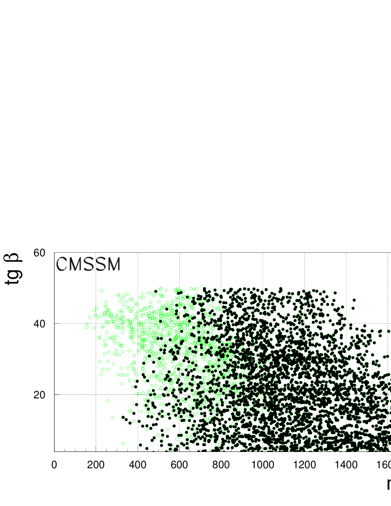
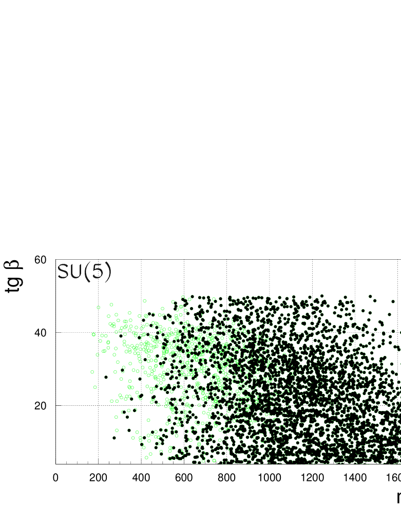
FIG. 1.: Mass of the charged Higgs boson vs $\tan\beta$ in the CMSSM and in the SU(5)–inspired MSSM. Black dots are points allowed by the $b\to s\gamma$ constraint while open circles fail to satisfy this constraint.

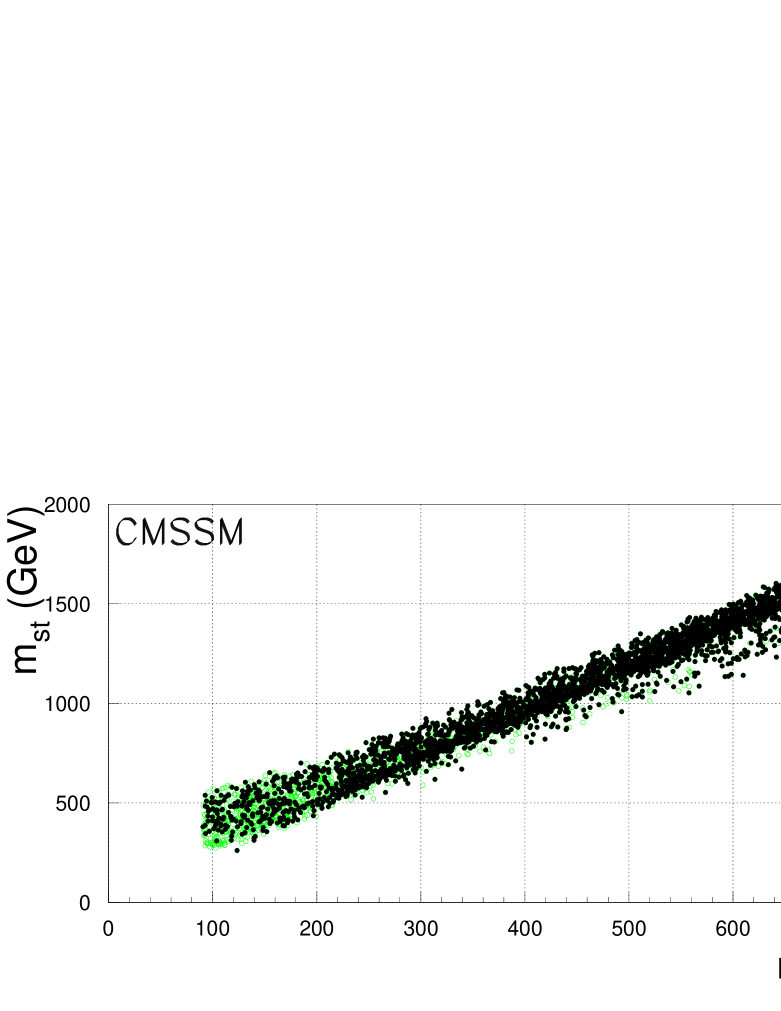
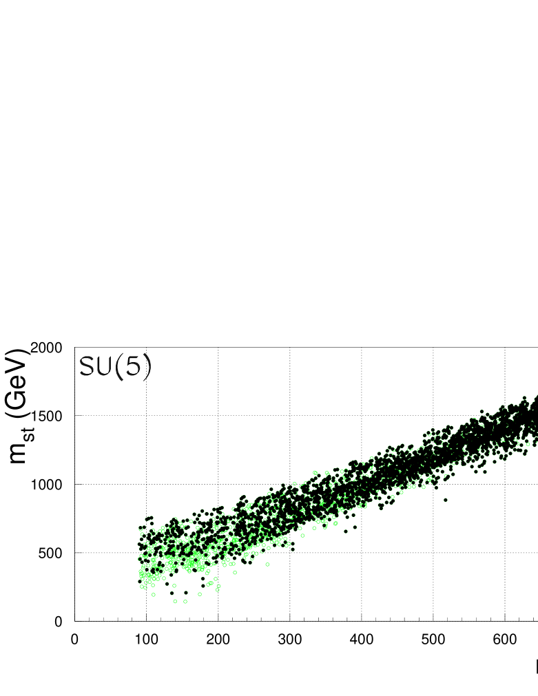
FIG. 2.: Chargino–stop mass correlation in the CMSSM and in the SU(5)–inspired MSSM. Black dots are points allowed by the $b\to s\gamma$ constraint while open circles fail to satisfy this constraint.

FIG. 3.: Values of the SUSY phases allowed by the EDM constraints, and $\phi_{\mu}$–$M_{0}$ correlation.

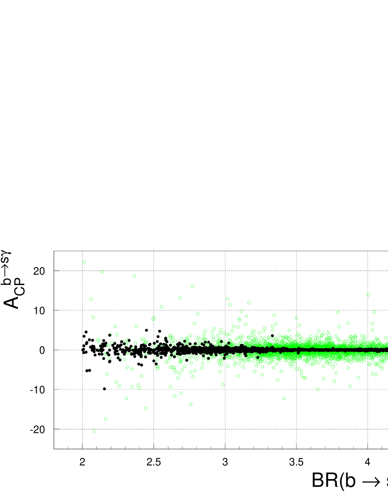
FIG. 4.: $CP$ asymmetry vs total width of the decay $b\rightarrow s\gamma$. The empty circles are computed without any restriction on the phases. The filled black ones show the impact of the EDM’s constraints.

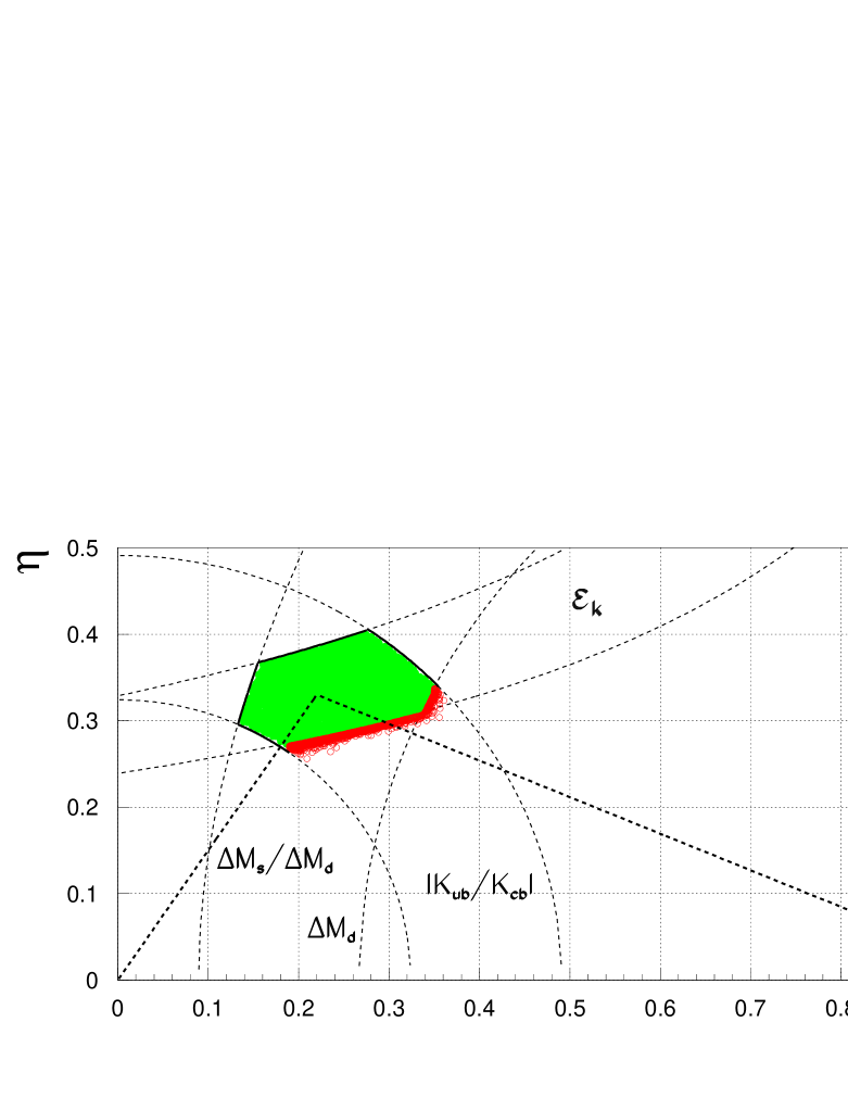
FIG. 5.: Fit of the unitary triangle in the flavor blind MSSM framework. The filled region corresponds to the SM fit and the open circles show the possible deviations that can occurr in these models.

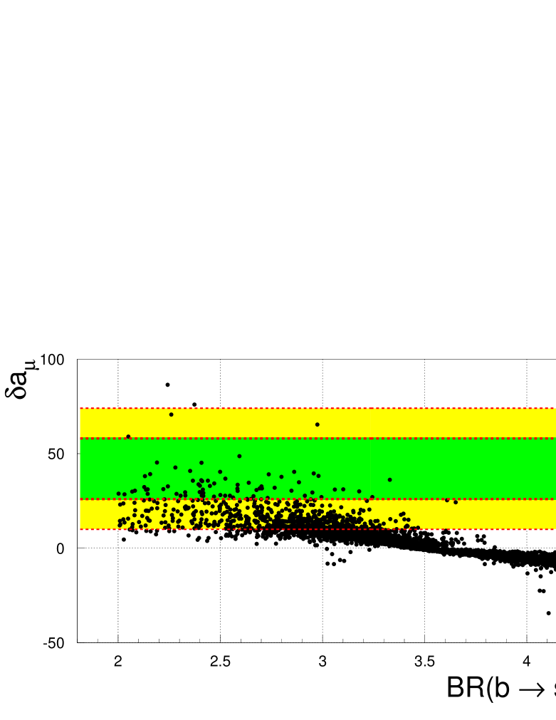
FIG. 6.: Plot of the SUSY contribution to $a_{\mu^{+}}$ versus the branching ratio of $b\rightarrow s\gamma$. The bands represent the $1\sigma$ and $2\sigma$ allowed regions according to Eq. (71).

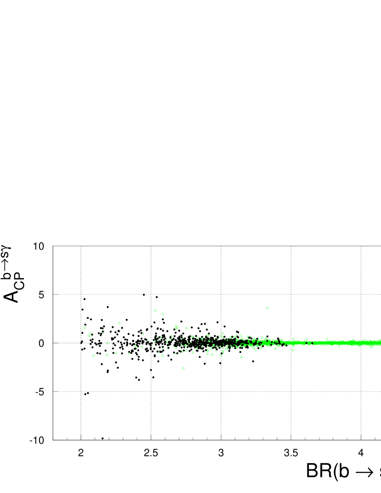
FIG. 7.: Plot of the $CP$ asymmetry versus the branching ratio of $b\rightarrow s\gamma$. We allow only for points whose phases satisfy the EDM’s constraints. The black dots satisfy the 2 sigma bound implied by Eq. (71).

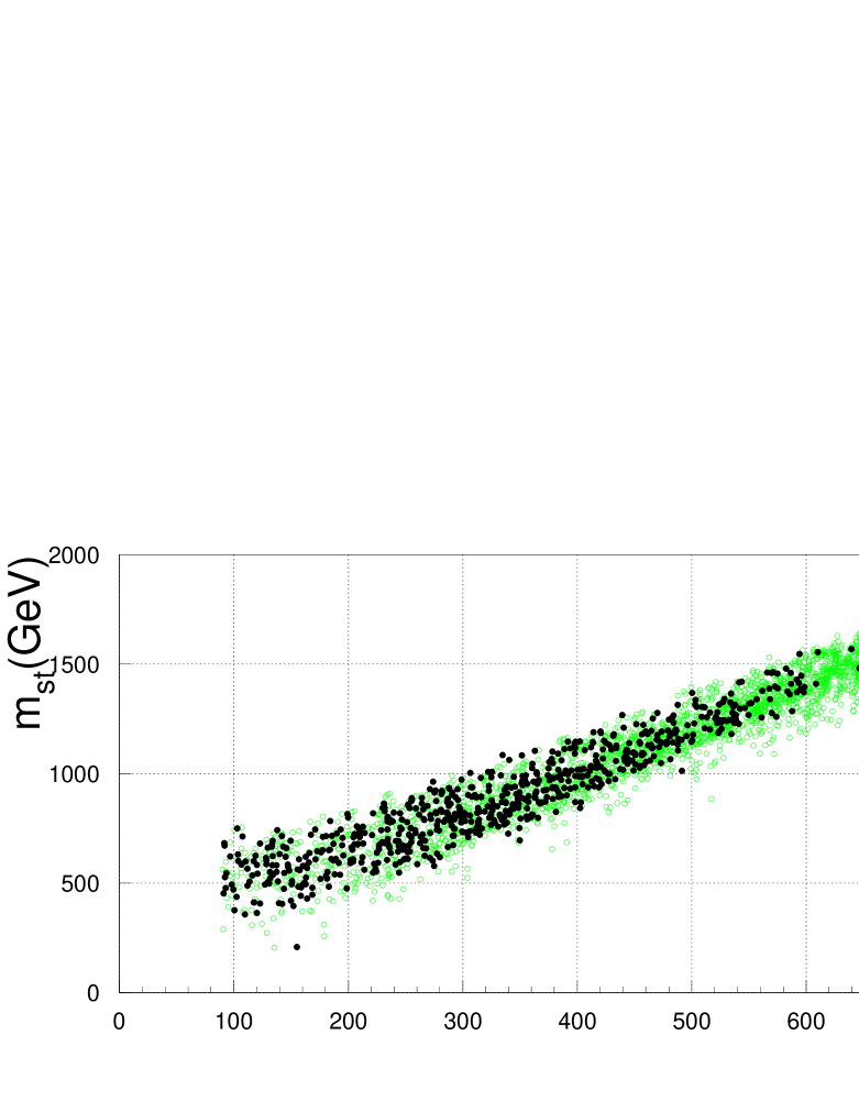
FIG. 8.: Impact of the $a_{\mu^{+}}$ constraint on the lightest chargino and stop masses. The black dots satisfy the 2 sigma bound implied by Eq. (71).

TABLE I.: Approximate solutions of third generation squark–mass parameters and Higgs mass parameters, $m^{2}_{i}=$ $c_{i1}M^{2}_{10}$ $+c_{i2}M^{2}_{5}$ $+c_{i3}M^{2}_{H1}$ $+c_{i4}M^{2}_{H2}$ $+c_{i5}M^{2}_{1/2}$ $+c_{6i}\mbox{Re}(A_{d}(0)M^{*}_{1/2})$ $+c_{i7}\mbox{Re}(A_{u}(0)M^{*}_{1/2})$ $+c_{8i}|A_{d}(0)|^{2}$$+c_{i9}|A_{u}(0)|^{2}$.

		$c_{i1}$	$c_{i2}$	$c_{i3}$	$c_{i4}$	$c_{i5}$	$c_{i6}$	$c_{i7}$	$c_{i8}$	$c_{i9}$
$\tan\beta=2.5$	$m^{2}_{D_{3}}$	0	1	0	0	6.14	0	0	0	0
	$m^{2}_{U_{3}}$	0.43	0	0	-0.28	3.94	0	0.18	0	-0.04
	$m^{2}_{Q_{3}}$	0.72	0	0	-0.14	5.49	0	0.09	0	-0.02
	$m^{2}_{H_{1}}$	0	0	1	0	0.36	0	0	0	0
	$m^{2}_{H_{2}}$	-0.85	0	0	0.58	-3.05	0	0.28	0	-0.06
$\tan\beta=5$	$m^{2}_{D_{3}}$	0	1	0	0	5.83	0.01	0	0	0
	$m^{2}_{U_{3}}$	0.49	0	0	-0.25	3.88	0	0.25	0	-0.06
	$m^{2}_{Q_{3}}$	0.74	0	0	-0.13	5.30	0	0.12	0	-0.03
	$m^{2}_{H_{1}}$	0	0	1	0	0.29	0.01	0	0	0
	$m^{2}_{H_{2}}$	-0.76	0	0	0.62	-2.76	0	0.37	0	-0.09
$\tan\beta=10$	$m^{2}_{D_{3}}$	-0.01	0.99	-0.01	0	5.77	0.03	0	-0.01	0
	$m^{2}_{U_{3}}$	0.50	0	0	-0.25	3.91	0	0.26	0	-0.06
	$m^{2}_{Q_{3}}$	0.75	0	0	-0.12	5.29	0.01	0.13	0	-0.03
	$m^{2}_{H_{1}}$	-0.01	-0.01	0.99	0	0.21	0.04	0	-0.01	0
	$m^{2}_{H_{2}}$	-0.75	0	0	0.63	-2.71	0	0.39	0	-0.09
$\tan\beta=30$	$m^{2}_{D_{3}}$	-0.08	0.92	-0.08	0	5.12	0.23	0	-0.06	0
	$m^{2}_{U_{3}}$	0.50	0	0	-0.25	3.93	0	0.26	0	-0.06
	$m^{2}_{Q_{3}}$	0.71	-0.04	-0.04	-0.12	4.97	0.12	0.13	-0.03	-0.03
	$m^{2}_{H_{1}}$	-0.14	-0.14	0.86	0	-0.77	0.37	0	-0.11	0
	$m^{2}_{H_{2}}$	-0.75	0	0	0.63	-2.66	0	0.39	0	-0.09
$\tan\beta=40$	$m^{2}_{D_{3}}$	-0.16	0.84	-0.16	0	4.46	0.32	0	-0.08	0
	$m^{2}_{U_{3}}$	0.49	0	0	-0.25	3.92	0	0.25	0	-0.06
	$m^{2}_{Q_{3}}$	0.66	-0.08	-0.08	-0.13	4.63	0.16	0.12	-0.04	-0.03
	$m^{2}_{H_{1}}$	-0.30	-0.30	0.70	0	-1.79	0.52	0	-0.17	0
	$m^{2}_{H_{2}}$	-0.76	0	0	0.62	-2.66	0	0.37	0	-0.09

TABLE II.: Approximate solutions of $|\mu|^{2}$ and $m_{A^{0}}$ in the CMSSM case: $m^{2}_{i}=c_{i1}M^{2}_{0}$ $+c_{i2}M^{2}_{1/2}+c_{3i}A_{0}M_{1/2}+c_{i4}A_{0}^{2}+c_{i5}$. $c_{i5}=-m^{2}_{Z}/2$ in case of $|\mu|^{2}$ and $m^{2}_{W}-m^{2}_{Z}$ in case of $m^{2}_{H^{+}}$.

$\tan\beta$		$c_{1}$	$c_{2}$	$c_{3}$	$c_{4}$
2.5	$|\mu|^{2}$	0.51	3.70	-0.33	0.08
	$m^{2}_{H^{+}}$	1.75	4.71	-0.38	0.09
5	$|\mu|^{2}$	0.19	2.89	-0.39	0.09
	$m^{2}_{H^{+}}$	1.23	3.30	-0.39	0.09
10	$|\mu|^{2}$	0.13	2.74	-0.40	0.10
	$m^{2}_{H^{+}}$	1.10	2.98	-0.36	0.08
30	$|\mu|^{2}$	0.12	2.66	-0.39	0.09
	$m^{2}_{H^{+}}$	0.69	1.89	-0.02	-0.02
40	$|\mu|^{2}$	0.15	2.66	-0.37	0.09
	$m^{2}_{H^{+}}$	0.24	0.87	0.15	-0.08

TABLE III.: Approximate solutions of $|\mu|^{2}$ and $m_{A^{0}}$ in the $SU(5)$ case: $m^{2}_{i}=c_{i1}M^{2}_{10}$ $+c_{i2}M^{2}_{5}+c_{i3}M^{2}_{H1}+c_{i4}M^{2}_{H2}+c_{i5}M^{2}_{1/2}+c_{6i}A_{d}(0)M_{1/2}+c_{i7}A_{u}(0)M_{1/2}+c_{8i}A^{2}_{d}(0)+c_{i9}A^{2}_{u}(0)+c_{i10}$. $c_{i10}=-m^{2}_{Z}/2$ in case of $|\mu|^{2}$ and $m^{2}_{W}-m^{2}_{Z}$ in case of $m^{2}_{H^{+}}$.

$\tan\beta$		$c_{1}$	$c_{2}$	$c_{3}$	$c_{4}$	$c_{5}$	$c_{6}$	$c_{7}$	$c_{8}$	$c_{9}$
2.5	$|\mu|^{2}$	1.01	0	0.19	-0.69	3.70	0	-0.33	0	0.08
	$m^{2}_{H^{+}}$	1.17	0	1.38	-0.80	4.71	0	-0.38	0	0.09
5	$|\mu|^{2}$	0.80	0	0.04	-0.64	2.89	0	-0.39	0	0.09
	$m^{2}_{H^{+}}$	0.82	0	1.08	-0.67	3.30	0.01	-0.40	0	0.10
10	$|\mu|^{2}$	0.75	0	0.01	-0.63	2.74	0	-0.40	0	0.10
	$m^{2}_{H^{+}}$	0.75	-0.01	1.01	-0.64	2.98	0.04	-0.40	-0.01	0.10
30	$|\mu|^{2}$	0.75	0	0	-0.63	2.66	0	-0.39	0	0.09
	$m^{2}_{H^{+}}$	0.60	-0.14	0.85	-0.63	1.89	0.37	-0.39	-0.11	0.09
40	$|\mu|^{2}$	0.76	0	0	-0.62	2.66	0	-0.37	0	0.09
	$m^{2}_{H^{+}}$	0.46	-0.30	0.70	-0.62	0.87	0.52	-0.37	-0.17	0.09

TABLE IV.: Approximate solutions of first generation squark–mass parameters, $m^{2}_{i}=b_{i1}M^{2}_{10}+b_{i2}M^{2}_{5}+b_{i3}M^{2}_{1/2}$

	$b_{i1}$	$b_{i2}$	$b_{i3}$
$m^{2}_{D_{1}}$	0	1	6.1
$m^{2}_{U_{1}}$	1	0	6.15
$m^{2}_{Q_{1}}$	1	0	6.5
$m^{2}_{E_{1}}$	1	0	0.15
$m^{2}_{L_{1}}$	0	1	1.5

TABLE V.: Approximate solutions of the A–parameters as a function of the GUT–parameters for various $\tan\beta$. All Parameters are given by $A_{i}=a_{i1}A_{d}(0)+a_{i2}A_{u}(0)+a_{i3}M_{1/2}$

	$\tan\beta=2.5$			$\tan\beta=5$			$\tan\beta=10$			$\tan\beta=30$			$\tan\beta=40$
	$a_{i1}$	$a_{i2}$	$a_{i3}$	$a_{i1}$	$a_{i2}$	$a_{i3}$	$a_{i1}$	$a_{i2}$	$a_{i3}$	$a_{i1}$	$a_{i2}$	$a_{i3}$	$a_{i1}$	$a_{i2}$	$a_{i3}$
$A_{u}$	0	0.58	-2.89	0	0.63	-2.88	0	0.63	-2.90	0	0.63	-2.92	0	0.62	-2.91
$A_{d}$	1	0	-3.74	1	0	-3.63	0.99	0	-3.61	0.86	0	-3.42	0.7	0	-3.15
$A_{t}$	0	0.15	-1.98	0	0.24	-2.09	0	0.25	-2.12	-0.04	0.25	-2.07	-0.08	0.24	-1.97
$A_{b}$	1	-0.14	-3.45	0.99	-0.13	-3.36	0.98	-0.12	-3.33	0.74	-0.12	-2.93	0.45	-0.13	-2.41

REFERENCES

- [1] S. P. Martin and M. T. Vaughn, Phys. Rev. D 50 (1994) 2282 [hep-ph/9311340].
- [2] D. M. Pierce, J. A. Bagger, K. Matchev and R. Zhang, Nucl. Phys. B 491 (1997) 3 [hep-ph/9606211].
-
[3]
T. Falk and K. A. Olive,
Phys. Lett. B 375, 196 (1996)
[hep-ph/9602299];
T. Ibrahim and P. Nath, Phys. Lett. B 418, 98 (1998) [hep-ph/9707409];
T. Ibrahim and P. Nath, Phys. Rev. D 57, 478 (1998) [hep-ph/9708456];
T. Ibrahim and P. Nath, Phys. Rev. D58, 111301 (1998) [hep-ph/9807501];
M. Brhlik, G.J. Good and G.L. Kane, Phys. Rev. D59, 115004 (1999) [hep-ph/9810457];
M. Brhlik, L. Everett, G.L. Kane and J. Lykken, Phys. Rev. Lett. 83, 2124 (1999) [hep-ph/9905215];
M. Brhlik, L. Everett, G.L. Kane and J. Lykken, Phys. Rev. D62, 035005 (2000) [hep-ph/9908326];
T. Ibrahim and P. Nath, Phys. Rev. D61, 093004 (2000) [hep-ph/9910553]. - [4] A. Bartl, T. Gajdosik, W. Porod, P. Stockinger and H. Stremnitzer, Phys. Rev. D 60 (1999) 073003 [hep-ph/9903402].
-
[5]
L. E. Ibañez and C. Lopez,
Nucl. Phys. B 233 (1984) 511;
L. E. Ibañez and J. Mas, Nucl. Phys. B 286 (1987) 107;
N. K. Falck, Z. Phys. C 30, 247 (1986). - [6] S. Bertolini, F. Borzumati, A. Masiero and G. Ridolfi, Nucl. Phys. B353, 591 (1991).
- [7] D. Kazakov and G. Moultaka, Nucl. Phys. B 577 (2000) 121 [hep-ph/9912271].
-
[8]
J. A. Casas, A. Lleyda and C. Munoz,
Nucl. Phys. B 471 (1996) 3
[hep-ph/9507294];
J. A. Casas and S. Dimopoulos, Phys. Lett. B 387, 107 (1996) [hep-ph/9606237]. - [9] D. E. Groom et al. [Particle Data Group Collaboration], Eur. Phys. J. C 15, 1 (2000).
-
[10]
S. Ahmed et al. (CLEO Collaboration),
CLEO CONF 99-10,
hep-ex/9908022;
K. Abe [Belle Collaboration], hep-ex/0103042. -
[11]
F. M. Borzumati and C. Greub,
Phys. Rev. D 58, 074004 (1998)
[hep-ph/9802391];
F. M. Borzumati and C. Greub, Phys. Rev. D 59, 057501 (1999) [hep-ph/9809438]. - [12] R. Garisto and J. N. Ng, Phys. Lett. B 315, 372 (1993) [hep-ph/9307301].
- [13] A. J. Buras, P. Gambino, M. Gorbahn, S. Jager and L. Silvestrini, Nucl. Phys. B592, 55 (2001) [hep-ph/0007313].
-
[14]
A. Ali and D. London,
Eur. Phys. J. C 9, 687 (1999)
[hep-ph/9903535];
A. Ali and D. London, Phys. Rept. 320, 79 (1999) [hep-ph/9907243]. -
[15]
M. Ciuchini, G. Degrassi, P. Gambino and G. F. Giudice,
Nucl. Phys. B 534, 3 (1998)
[hep-ph/9806308];
A. Brignole, F. Feruglio and F. Zwirner, Z. Phys. C 71, 679 (1996) [hep-ph/9601293];
M. Misiak, S. Pokorski and J. Rosiek, hep-ph/9703442. - [16] M. Brhlik, L. Everett, G. L. Kane, S. F. King and O. Lebedev, Phys. Rev. Lett. 84, 3041 (2000) [hep-ph/9909480].
- [17] H. N. Brown et al. [Muon g-2 Collaboration], hep-ex/0102017.
- [18] A. Czarnecki and B. Krause, Phys. Rev. Lett. 78, 4339 (1997) [hep-ph/9704355].
- [19] I. S. Altarev et al., Phys. Lett. B 276, 242 (1992).
- [20] I. S. Altarev et al., Phys. Atom. Nucl. 59, 1152 (1996).
- [21] J. P. Jacobs, W. M. Klipstein, S. K. Lamoreaux, B. R. Heckel, and E. N. Fortson Phys. Rev. Lett. 71 (1993) 3782, Phys. Rev. A 52 (1995) 3521.
-
[22]
E. D. Commins, S. B. Ross, D. DeMille and B. C. Regan,
Phys. Rev. A 50, 2960 (1994);
E. D. Commins, Eur. Phys. J. C 3, 620 (1998). -
[23]
W. Buchmüller and D. Wyler,
Phys. Lett. B121, 321 (1983);
J. Polchinski and M. Wise, Phys. Lett. B125, 393 (1983);
W. Fischler, S. Paban and S. Thomas, Phys. Lett. B289, 373 (1992) [hep-ph/9205233]. -
[24]
S. Dimopoulos and G.F. Giudice, Phys. Lett. B357, 573 (1995)
[hep-ph/9507282];
A. Cohen, D.B. Kaplan and A.E. Nelson, Phys. Lett. B388, 588 (1996) [hep-ph/9607394];
A. Pomarol and D. Tommasini, Nucl. Phys. B466, 3 (1996) [hep-ph/9507462]. -
[25]
S. Baek and P. Ko,
Phys. Rev. Lett. 83, 488 (1999)
[hep-ph/9812229];
S. Baek and P. Ko, Phys. Lett. B462, 95 (1999) [hep-ph/9904283]. - [26] D. Demir, A. Masiero and O. Vives, Phys. Rev. Lett. 82, 2447 (1999), Err. ibid. 83, 2093 (1999) [hep-ph/9812337].
- [27] D. Chang, W. Keung and A. Pilaftsis, Phys. Rev. Lett. 82, 900 (1999) [hep-ph/9811202].
-
[28]
S.A. Abel and J.M. Frere, Phys. Rev. D55, 1623 (1997)
[hep-ph/9608251];
S. Khalil, T. Kobayashi and A. Masiero, Phys. Rev. D60, 075003 (1999) [hep-ph/9903544];
S. Khalil and T. Kobayashi, Phys. Lett. B460, 341 (1999) [hep-ph/9906374]. - [29] S. Khalil, T. Kobayashi and O. Vives, Nucl. Phys. B 580, 275 (2000) [hep-ph/0003086].
-
[30]
J. Bagger, J. L. Feng and N. Polonsky,
Nucl. Phys. B 563, 3 (1999)
[hep-ph/9905292];
J. L. Feng, K. T. Matchev and T. Moroi, Phys. Rev. Lett. 84, 2322 (2000) [hep-ph/9908309]. - [31] A. Manohar and H. Georgi, Nucl. Phys. B 234, 189 (1984).
- [32] J. Ellis and R. A. Flores, Phys. Lett. B 377, 83 (1996) [hep-ph/9602211].
- [33] M. Pospelov and A. Ritz, Phys. Rev. D 63, 073015 (2001) [hep-ph/0010037].
- [34] T. Falk, K. A. Olive, M. Pospelov and R. Roiban, Nucl. Phys. B 560, 3 (1999) [hep-ph/9904393].
- [35] S. Abel, S. Khalil and O. Lebedev, hep-ph/0103031.
- [36] V. Barger, T. Falk, T. Han, J. Jiang, T. Li and T. Plehn, hep-ph/0101106.
- [37] N. Ghodbane, S. Katsanevas, I. Laktineh and J. Rosiek, hep-ph/0012031.
- [38] F. Gabbiani, E. Gabrielli, A. Masiero and L. Silvestrini, Nucl. Phys. B477, 321 (1996) [hep-ph/9604387].
- [39] K. Chetyrkin, M. Misiak and M. Munz, Phys. Lett. B 400, 206 (1997) [hep-ph/9612313].
- [40] M. Ciuchini, G. Degrassi, P. Gambino and G. F. Giudice, Nucl. Phys. B 527, 21 (1998) [hep-ph/9710335].
- [41] F. Borzumati, C. Greub, T. Hurth and D. Wyler, Phys. Rev. D 62, 075005 (2000) [hep-ph/9911245].
- [42] G. Degrassi, P. Gambino and G. F. Giudice, JHEP0012, 009 (2000) [hep-ph/0009337].
- [43] M. Carena, D. Garcia, U. Nierste and C. E. Wagner, Phys. Lett. B 499 (2001) 141.
- [44] W. de Boer, M. Huber, A. V. Gladyshev and D. I. Kazakov, hep-ph/0102163.
-
[45]
H.E. Haber and G.L Kane,
Phys. Rept. 117, 75 (1985);
H. P. Nilles, Phys. Rept. 110, 1 (1984). - [46] A.L. Kagan and M. Neubert, Eur. Phys. J. C7, 5 (1999) [hep-ph/9805303].
- [47] J. M. Soares, Nucl. Phys. B367, 575 (1991).
- [48] D. A. Demir, A. Masiero and O. Vives, Phys. Lett. B479, 230 (2000), [hep-ph/9911337].
- [49] D. Demir, A. Masiero and O. Vives, Phys. Rev. D61, 075009 (2000) [hep-ph/9909325].
- [50] C. Chua, X. He and W. Hou, Phys. Rev. D 60, 014003 (1999) [hep-ph/9808431].
- [51] M. Aoki, G. Cho and N. Oshimo, Nucl. Phys. B554, 50 (1999) [hep-ph/9903385].
-
[52]
T. Goto, Y. Okada, Y. Shimizu and M. Tanaka,
Phys. Rev. D 55, 4273 (1997)
[hep-ph/9609512];
T. Goto, Y. Y. Keum, T. Nihei, Y. Okada and Y. Shimizu, Phys. Lett. B460, 333 (1999) [hep-ph/9812369]. - [53] A.L. Kagan and M. Neubert, Phys. Rev. D58, 094012 (1998) [hep-ph/9803368].
- [54] P. Cho, M. Misiak and D. Wyler, Phys. Rev. D 54 (1996) 3329.
- [55] A. Ali, P. Ball, L. T. Handoko and G. Hiller, Phys. Rev. D 61 (2000) 074024.
- [56] E. Lunghi, A. Masiero, I. Scimemi and L. Silvestrini, Nucl. Phys. B 568 (2000) 120.
- [57] A. Masiero and O. Vives, Phys. Rev. Lett. 86, 26 (2001) [hep-ph/0007320].
- [58] A. Masiero, M. Piai and O. Vives, hep-ph/0012096.
- [59] A. J. Buras, P. Gambino, M. Gorbahn, S. Jager and L. Silvestrini, Phys. Lett. B 500, 161 (2001) [hep-ph/0007085].
-
[60]
G. C. Branco, G. C. Cho, Y. Kizukuri and N. Oshimo,
Phys. Lett. B 337, 316 (1994)
[hep-ph/9408229];
G. C. Branco, G. C. Cho, Y. Kizukuri and N. Oshimo, Nucl. Phys. B 449, 483 (1995). - [61] T. Kobayashi and O. Vives, hep-ph/0011200.
-
[62]
R. Barbieri, R. Contino and A. Strumia,
Nucl. Phys. B 578, 153 (2000)
[hep-ph/9908255];
K. S. Babu, B. Dutta and R. N. Mohapatra, Phys. Rev. D 61, 091701 (2000) [hep-ph/9905464];
A. Masiero and H. Murayama, Phys. Rev. Lett. 83, 907 (1999) [hep-ph/9903363]. - [63] A. J. Buras and R. Buras, Phys. Lett. B 501, 223 (2001) [hep-ph/0008273].
- [64] A. Czarnecki and W. J. Marciano, Nucl. Phys. (Proc. Suppl.) B 76 (1999) 245.
- [65] M. Davier and A. Hocker, Phys. Lett. B 435 (1998) 427.
- [66] A. Czarnecki and W. J. Marciano, hep-ph/0102122.
- [67] F. J. Yndurain, hep-ph/0102312.
- [68] T. Moroi, Phys. Rev. D 53 (1996) 6565.
-
[69]
T. Ibrahim and P. Nath,
Phys. Rev. D 62, 015004 (2000)
[hep-ph/9908443];
T. Ibrahim and P. Nath, Phys. Rev. D 61, 095008 (2000) [hep-ph/9907555]. - [70] L. Everett, G. L. Kane, S. Rigolin and L. Wang, hep-ph/0102145.
- [71] J. L. Feng and K. T. Matchev, hep-ph/0102146.
- [72] E. A. Baltz and P. Gondolo, hep-ph/0102147.
- [73] U. Chattopadhyay and P. Nath, hep-ph/0102157.
- [74] S. Komine, T. Moroi and M. Yamaguchi, hep-ph/0102204.
- [75] J. Ellis, D. V. Nanopoulos and K. A. Olive, hep-ph/0102331.
- [76] S. P. Martin and J. D. Wells, hep-ph/0103067.
- [77] D. F. Carvalho, J. Ellis, M. E. Gomez and S. Lola, hep-ph/0103256.
- [78] H. Baer, C. Balazs, J. Ferrandis and X. Tata, hep-ph/0103280.
- [79] A. Bartl, H. Fraas, W. Majerotto and N. Oshimo, Phys. Rev. D 40, 1594 (1989).