Atmospheric neutrino flux supported by recent muon experiments

Abstract

We present a new one-dimensional calculation of low and intermediate energy atmospheric muon and neutrino fluxes, using up-to-date data on primary cosmic rays and hadronic interactions. We study several sources of uncertainties relevant to our calculations. A comparison with the muon fluxes and charge ratios measured in several modern balloon-borne experiments suggests that the atmospheric neutrino flux is essentially lower than one used for the standard analyses of the sub-GeV and multi-GeV neutrino induced events in underground detectors.

INFNFE-01-01

, ,

1 Introduction

The atmospheric neutrino (AN) flux is one of the main tools for studying neutrino oscillations, neutrino decay and nonstandard neutrino-matter interactions. Furthermore it represents an unavoidable background for key experiments in astroparticle physics, as those searching for proton decay, $n-\overline{n}$ transitions in nuclei, etc. Therefore, the accuracy of theoretical predictions of the AN flux ultimately affects the interpretation of many experimental data.

After several studies performed in the frameworks of one-dimensional (1D) [1, 2, 3] and three-dimensional (3D) [4, 5, 6] cascade models, the physics of neutrino production in the sub- and multi-GeV energy ranges is fairly well understood. However, the validity of the AN flux calculations is still controversial. This is mainly related to the uncertainties in the required input data (inclusive cross sections for particle production, primary cosmic ray spectrum and composition, etc.). Moreover, the problem is too complex to be solved without many simplifications (explicit or implicit) and these also are essential sources of uncertainties in the predicted AN fluxes [7, 8, 9, 10]. A popular opinion is that the accuracy of the present-day calculations of the low-energy AN flux is about 20–30%. Sometimes this belief of obscure origin is treated as the uncertainty in the normalization factor. But, as a matter of fact, the uncertainties in the input data are so large that the actual accuracy of the AN flux turns out to be much worse. It is also essential that the uncertainties are very energy dependent and therefore they cannot be reduced to a simple renormalization.

In this work we present a new 1D calculation of low and intermediate energy muon and neutrino fluxes, based on up-to-date data on primary cosmic-ray flux and hadronic interactions. Our calculation is based on a kinetic approach. In order to check the validity of our description of hadronic interactions and shower development, we perform a comparison of the predicted atmospheric muon fluxes with the data from several recent balloon-borne experiments.

We believe that an accurate 1D AN flux calculation is still helpful, despite the results of 3D calculations are now available. Indeed, the main lessons we got from the recent 3D analyses [5, 6, 8, 9] may be summarized as follows.

• 3D effects lead to a strong modification of zenith and azimuth angle distributions of neutrinos at energies $E_{\nu}\lesssim 0.5$ GeV. On the other hand, the corresponding effect for the neutrino-induced events in underground detectors is expected to be modest and scarcely measurable, because their distributions are close to isotropic out of a very big mean scattering angle in quasielastic neutrino-nucleus collisions at low energies.

• Even at very low energies the 3D corrections to the $4\pi$ and even $2\pi$ averaged AN fluxes are relatively small. At least, they are comparable with the uncertainties in the input data, including the uncertainties in the cross sections for exclusive neutrino-nucleus interactions needed for simulating the neutrino-induced events in the underground detectors.

• Above $1-2$ GeV the 3D effects become negligible for the neutrino fluxes averaged over the azimuth angles at any zenith angle.

On that ground, we expect the calculation offered for consideration to be valid without restrictions at $E_{\nu}\gtrsim 1$ GeV and we consider it as a basis for future 3D generalization of our approach to the AN problem.

Furthermore, our 1D code is useful for testing 1D and 3D codes with a method completely different from Monte Carlo. It can be used to perform a systematic analysis of uncertainties in the AN flux calculations and to adjust some poorly known input parameters, using the data on cosmic-ray secondaries. In this work, in order to evaluate quantitatively the uncertainties related to the particle interactions, we perform a comparison of the results obtained with different models for meson production in nucleon-nucleus and nucleus-nucleus collisions.

2 The CORT code

The present work is based on an updated code CORT (Cosmic-Origin Radiation Transport), previously developed in [11] and used in [1] (see also [12, 13]). Like the earlier version, the current Fortran 90 code implements a numerical solution of a system of 1D kinetic equations describing the propagation of nuclei, nucleons, light mesons, muons and (anti)neutrinos of low and intermediate energies through a spherical, nonisothermal atmosphere. It takes into account solar modulation and geomagnetic effects, energy loss of charged particles, muon polarization and depolarization effect. The exact kinematics is used in description of particle interactions and decays. Let us sketch some most distinctive aspects.

In order to evaluate geomagnetic effects and to take into account the anisotropy of the primary cosmic-ray flux in the vicinity of the Earth, we use the method of ref. [11] and detailed maps of the effective vertical cutoff rigidities from ref. [14]. The maps are corrected for the geomagnetic pole drift and compared with the later results reviewed by Smart and Shea [15] and with the recent data on the proton flux in near earth orbit obtained with the Alpha Magnetic Spectrometer (AMS) [16]. The interpolation between the reference points of the maps is performed by means of two-dimensional local B-spline. The Quenby-Wenk relation (see e.g. [14]), re-normalized to the vertical cutoffs, is applied for evaluating the effective cutoffs for oblique directions. More sophisticated effects, like the short-period variations of the geomagnetic field, Forbush decrease, re-entrant cosmic-ray albedo contribution, etc., are neglected. We also neglect the geomagnetic bending of the trajectories of charged secondaries and multiple scattering effects. Validity of our treatment of secondary nucleons and nuclei was confirmed using all available data on proton spectra in the atmosphere (see [11]).

The meteorological effects are included using the Dorman model of the atmosphere [17] which assumes an isothermal stratosphere and constant gradient of temperature (as a function of depths) below the tropopause. Ionization, radiative and photonuclear muon energy losses are treated as continuous processes. This approximation is quite tolerable for atmospheric depths $h\lesssim 2\times 10^{3}$ g/cm² at all energies of interest [18]. Propagation of $\mu^{+}$ and $\mu^{-}$ originating from every source (pion or kaon decay) is described by separate kinetic equations for muons with definite polarization at production. These equations automatically account for muon depolarization through the energy loss (but not through the Coulomb scattering).

In the new version, essentially all approximate formulas used in [1, 11, 12, 13] are replaced (or duplicated for a control) with the more accurate numerical equivalents.

3 Primary cosmic ray spectrum and composition

In the present calculations, the nuclear component of primary cosmic rays is broken up into 5 principal groups: H, He, CNO, Ne-S and Fe with average atomic masses $A$ of 1, 4, 15, 27 and 56, respectively. We do not take into account the isotopic composition of the primary nuclei and assume $Z=A/2$ for $A>1$, since the expected effect on the secondary lepton fluxes is estimated to be small with respect to present-day experimental uncertainties in the absolute cosmic-ray flux and chemical composition.

We use the following 9-parameter model for the differential energy spectra of every nuclear group at the top of the atmosphere

$$\frac{\d F_{\mathrm{A}}(E)}{\d E}=\left\{\begin{matrix}F_{\mathrm{A}}^{1}\epsilon_{\mathrm{A}}^{-\Gamma_{\mathrm{A}}(\epsilon_{\mathrm{A}})}&\mbox{at}&E<W_{\mathrm{A}},\\ F_{\mathrm{A}}^{2}\epsilon_{\mathrm{A}}^{-\gamma_{\mathrm{A}}}&\mbox{at}&E>W_{\mathrm{A}},\end{matrix}\right.$$ (1)

with

$$\Gamma_{\mathrm{A}}(\epsilon_{\mathrm{A}})=\sum_{k=0}^{3}\gamma_{\mathrm{A}}^{(k)}\ln^{k}\epsilon_{\mathrm{A}},\quad\epsilon_{\mathrm{A}}={r_{\mathrm{A}}E}/{W_{\mathrm{A}}}.$$ (2)

Here $E$ is the total energy in GeV/nucleon. The condition for continuity of the spectrum and its first derivative in the point $E=W_{\mathrm{A}}$ yields

$$\ln\left(F_{\mathrm{A}}^{2}/F_{\mathrm{A}}^{1}\right)=\sum_{k=1}^{3}k\gamma_{\mathrm{A}}^{(k)}\ln^{k+1}r_{\mathrm{A}},\quad\gamma_{\mathrm{A}}=\sum_{k=0}^{3}(k+1)\gamma_{\mathrm{A}}^{(k)}\ln^{k}r_{\mathrm{A}}.$$

Thus, we remain with 7 independent parameters for each group which we determine by fitting the experimental data.

For the hydrogen and helium groups at $E<120$ GeV/nucleon we chose the data of the balloon-borne experiment BESS obtained by a flight in 1998 [19] (a period close to a minimum of solar activity). For higher energies (but below the knee) we use data by a series of twelve balloon flights of JACEE [20] and the result of an analysis by Wiebel-Sooth et al. [21] based upon a very representative compilation of world data on primaries and solid theoretical considerations. Since the fits obtained in [21] turned out to be very close to the combined result of the JACEE experiments, we call our model “BESS+JACEE” fit. A maximum likelihood analysis with $W_{1}=W_{4}=2$ TeV/nucleon gives the following values for the remaining parameters in eqs. (1) and (2):

$$F_{1}^{1} =5.7216\!\times\!10^{-5}, \quad F_{4}^{1} =1.6500\!\times\!10^{-7},$$

$$F_{1}^{2} =5.8511\!\times\!10^{-5}, \quad F_{4}^{2} =1.7239\!\times\!10^{-7},$$

$$r_{1} =1.5952, \quad r_{4} =0.4783,$$

$$\gamma_{1} =2.800, \quad\gamma_{4} =2.655,$$

$$\gamma_{1}^{(0)} =2.7119, \quad\gamma_{4}^{(0)} =2.7881,$$

$$\gamma_{1}^{(1)} =6.9771\!\times\!10^{-2}, \quad\gamma_{4}^{(1)} =1.1953\!\times\!10^{-1},$$

$$\gamma_{1}^{(2)} =3.2396\!\times\!10^{-2}, \quad\gamma_{4}^{(2)} =2.8694\!\times\!10^{-2},$$

$$\gamma_{1}^{(3)} =3.8561\!\times\!10^{-3}, \quad\gamma_{4}^{(3)} =2.0829\!\times\!10^{-3},$$

where $F_{\mathrm{A}}^{i}$ are in m^-2s^-1sr^-1(GeV/nucleon)^-1. Clearly the many digits in the above parameters are by no means indicating the accuracy of the data, but they are necessary to avoid loss of accuracy in numerical calculations.

Figure 1 shows a comparison between the BESS+JACEE fit, the data from [19, 20], the fit from [21] (shaded areas) and several other experiments [22, 23, 24, 25, 26, 27, 28, 29, 30, 31, 32], performed in different periods of solar activity. The filled/shaded areas in fig. 1 represent the power-type parametrizations derived in[20, 22, 24, 28, 31, 32] from the original data. The legend indicates the publication dates and (when relevant) the years of measurements.

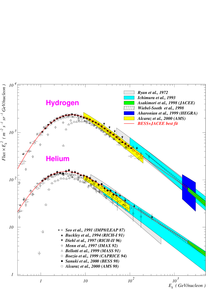
Figure 1: Differential proton and helium spectra as a function of kinetic energy per nucleon. The data points and filled/shaded areas are from [19, 20, 21, 22, 23, 24, 25, 26, 27, 28, 29, 30, 31, 32]. Solid curves represent the BESS+JACEE best fit (see text).

One sees that the BESS+JACEE fit is in excellent agreement with the recent AMS data on the proton flux [31]. On the other hand it slightly exceeds the AMS helium flux [32] (with average discrepancy of about 15%). Our choice of the BESS 98 data was in particular conditioned by the fact that the power-law extrapolation of the high-energy tail of the AMS helium rigidity spectrum ($\propto R^{-(2.74\pm 0.02)}$) [32] distinctly worse joins the world-averaged fit ($\propto E^{-(2.64\pm 0.02)}$) [21] and even the JACEE 1-12 fit ($\propto E^{-\left(2.68^{+0.04}_{-0.06}\right)}$) [20].

We assume that the spectra of the remaining three nuclear groups are similar to the helium spectrum,

$$\frac{\d F_{\mathrm{A}}(E)}{\d E}=c_{A}\frac{\d F_{\mathrm{4}}(E)}{\d E}\quad(\mathrm{A}=15,27,56).$$

This assumption does not contradict the world data for the CNO and Ne-S nuclear groups but works a bit worse for the iron group. Nevertheless, a more sophisticated model would be unpractical since the corresponding correction would affect the secondary lepton fluxes by a negligible margin. A normalization using the relevant data yields $c_{15}=0.068$, $c_{27}=0.026$, $c_{56}=0.0054$.

In this paper we do not consider the effects of solar modulation and use the BESS+JACEE spectrum in all calculations. Therefore the predicted muon and neutrino fluxes are to some extent the maximum ones possible within our 1D cascade model.

4 Nucleon-nucleus and nucleus-nucleus interactions

Calculations with the earlier version of CORT [1, 11, 12, 13] were based on semiempirical models for inclusive nucleon and light meson production in collisions of nucleons with nuclei, proposed by Kimel’ and Mokhov (KM) [33] and by Serov and Sychev (SS) [34] (see also [35, 36] for the most recent versions). The KM model is valid for projectile nucleon momenta above $\sim 4$ GeV/c and for the secondary nucleon, pion and kaon momenta above 450, 150 and 300 MeV/c, respectively. Outside these ranges (that is mainly within the region of resonance production of pions) the SS model was used. Comparison of the KM model with the data and with some other models is discussed in [7, 37].

Both models are in essence comprehensive parametrizations of the relevant accelerator data. In our opinion, the combined “KM+SS” model provides a rather safe and model-independent basis to the low-energy atmospheric muon and neutrino calculations. However it is not free of uncertainties. For the present calculation, the fitting parameters of the KM model for meson and nucleon production off different nuclear targets were updated using accelerator data not available for the original analysis [33, 35]. The values of the parameters were extrapolated to the air nuclei (N, O, Ar, C). The overall correction is less than 10-15% within the kinematic regions significant to atmospheric cascade calculations. Besides, energy-dependent correction factors were introduced into the model to tune up the output $\pi^{+}/\pi^{-}$ ratio taking into account the relevant new data. This correction only slightly affects the total meson multiplicities and modifies the pion charge ratio within 5-9%.

The processes of meson regeneration and charge exchange ($\pi^{\pm}+\mathrm{Air}\to\pi^{\pm(\mp)}+X$ etc.) are not of critical importance for production of leptons with energies of our interest and can be considered in a simplified way. Here we use a proper renormalization of the meson interaction lengths, which was deduced from the results of ref. [38] obtained for high-energy cascades.

The next important ingredient of any cascade calculations is a model for nucleus-nucleus collisions. The overwhelming majority of muon and neutrino flux predictions is based on the simplest superposition model (SM) in which the collision of a nucleus A, with total energy $E_{\mathrm{A}}$ and atomic weight $A$, against a target nucleus B, is treated as the superposition of $A$ independent collisions of nucleons with the target nucleus, each nucleon having an energy $E_{0}=E_{\mathrm{A}}/A$. This approximation is based on the hypothesis that, when the energy per nucleon of the projectile is much larger than the single nucleon binding energy, the $A$ nucleons interact incoherently. Generally speaking, this approach is rather far from reality and its applicability to the lepton flux calculations is not evident. A more accurate treatment of nucleus-nucleus collisions becomes especially important at low energies and for the regions or directions with high geomagnetic cutoffs. Indeed, the magnetic rigidity of a proton bounded in a nucleus is a factor $A/Z$ larger than that of a free proton of the same energy and therefore (considering the steepness of the primary spectrum) mainly nuclei are responsible for production of the low-energy secondaries.

Here we consider a modest generalization of a simple “Glauber-like” model used in [1, 11, 12]. Namely, we write the inclusive spectrum of secondary particles $c$ ($c=p$, $n$, $\pi^{\pm}$, $K^{\pm}$, $K^{0},\ldots$) produced in AB collisions as

$$\frac{\d N_{\mathrm{AB}\to cX}}{\d x}= \xi_{\mathrm{AB}}^{c}\left[Z\frac{\d N_{p\mathrm{B}\to cX}}{\d x}+(A-Z)\frac{\d N_{n\mathrm{B}\to cX}}{\d x}\right]$$

$$+\left(1-\xi_{\mathrm{AB}}^{c}\right)\left[Z\delta_{cp}+(A-Z)\delta_{cn}\right]\delta(1-x).$$ (3)

Here $\d N_{N\mathrm{B}\to cX}/\d x$ is the spectrum of particles $c$ produced in $N\mathrm{B}$ collisions ($N=p,n$) and $\xi_{\mathrm{AB}}^{c}$ is the average fraction of inelastically interacting nucleons of the projectile nucleus A. The term proportional to delta function describes the contribution of “spectator” nucleons from the projectile nucleus.

In the standard Glauber-Gribov multiple scattering theory the quantity $\xi_{\mathrm{AB}}^{c}$ is certainly independent of the type of inclusive particle $c$. On the other hand, it depends of the type of nucleus collision. Indeed, essentially all nucleons participate in the central AB collisions ($\xi_{\mathrm{AB}}^{c}\simeq 1$) while, according to the well-known Bialas–Bleszyński–Czyż (BBC) relation [39],

$$\xi_{\mathrm{AB}}^{c}=\sigma_{N\mathrm{B}}^{\mathrm{inel}}/\sigma_{\mathrm{AB}}^{\mathrm{inel}}$$ (4)

for the minimum bias collisions.

To use (4) in a cascade calculation one should take into account that nucleons and mesons are effectively produced in nuclear collisions of different kind. Namely, the contribution from central collisions is almost inessential for the nucleon component of the cascade but quite important for light meson production. Thus one can expect that effectively $\xi_{\mathrm{AB}}^{\pi,K}>\xi_{\mathrm{AB}}^{p,n}$.

From now on we use relation (4) for nucleon production by any nucleus while for meson production we put $\xi_{\mathrm{He-Air}}^{\pi,K}=\xi$ and vary the parameter $\xi$ from 0.517 (the BBC value) to 0.710 (an experimental upper limit derived from the data on interactions of $\alpha$ particles with light nuclei [40]). Similar (within $\pm 15$%) variations of the parameters $\xi_{\mathrm{A-Air}}^{\pi,K}$ for other nuclear groups lead to very small effects on the muon and neutrino fluxes; we do not discuss these effects below.

It is evident that the SM corresponds to the formal limit $\xi_{\mathrm{AB}}^{c}=1$ in eq. (4), if one simultaneously puts $\sigma_{\mathrm{AB}}^{\mathrm{inel}}=\sigma_{N\mathrm{B}}^{\mathrm{inel}}$ in the transport equations for the nuclei and mesons. Below, we use this approximation making efforts to represent the results of the Bartol code [2] which is based on the TARGET model for meson production and the SM for collisions of nuclei.

5 Numerical results: muon fluxes

In order to test the validity of our description of hadronic interactions and shower development, we compare in this section some numerical results for muon fluxes with data from several recent balloon-borne experiments. Moreover, in order to evaluate quantitatively theoretical uncertainties, we compare the calculations obtained by using different codes and/or interaction models. Namely, we consider numerical results obtained with:
i) the CORT code, using our “standard” (KM+SS) interaction model;
ii) the CORT code, using the TARGET model for $\pi/K$ meson production (below, we refer to this calculation as “CORT+TARGET”).
iii) the original Bartol Monte Carlo code [2] with the same (BESS+JACEE) fit for the primary spectra (“TARGET”).

In fig. 2 we compare the $\mu^{-}$ fluxes calculated with the three mentioned models for twelve atmospheric ranges with the data of the balloon-borne experiment CAPRICE 94 [41]. The measurements were performed during ground runs in Lynn Lake ($h=10^{3}$ g/cm²) and during the continuous ascension of the balloon to its float altitude ($h\approx 4$ g/cm²). The nominal geomagnetic cutoff rigidity $R_{c}$ was about 0.5 GV and the detection cone opening was of about $20^{\circ}$ around the vertical direction with the typical zenith angle of $9^{\circ}$. The values of depths indicated in fig. 2 are the Flux-weighted Average Depths (FAD) [41] for eleven atmospheric ranges $\Delta h_{i}$ ($h_{i}<10^{3}$ g/cm²).

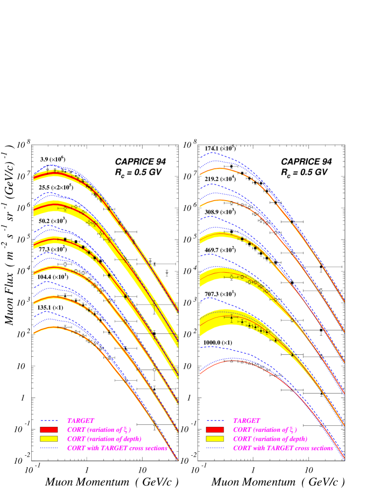
Figure 2: Differential momentum spectra of negative muons for different atmospheric depths. The data points are from the balloon-borne experiment CAPRICE 94 [41]. The curves and filled areas are the results of calculations with CORT and TARGET (see text). The numbers over the curves indicate the flux-weighted average atmospheric depths (in g/cm²) and scale factors.

Figure 2 contains many data. In order to make it easily readable, let us explain the notation in detail. The solid curves represent the results of our calculations for each FAD. They are obtained with the standard CORT and with $\xi$ varying between the limits mentioned in section 4, that is within $\pm 15$%. The thickness of the curves reflects the indetermination in the parameter $\xi$. For obvious reasons, the muon flux uncertainty due to this indetermination is maximal at the top of the atmosphere (it is about 15% at $h=3.9$ g/cm² and $p=100$ MeV/c) and becomes almost negligible for $h\gtrsim 100$ g/cm². The wide filled areas display the variations of the muon fluxes inside the ranges $\Delta h_{i}$. It is important to note that the thickness of the bands is relatively small just for the region of effective muon and neutrino production that is in the neighborhood of the broad maxima of the muon flux ($100-300$ g/cm²). This means that, in this region, the evaluation of the FAD cannot introduce any relevant uncertainty. Outside the region of effective production of leptons, the amplitude of the muon flux variations increases with decreasing muon momenta on account for the strong dependence of the meson production rate upon the depth at $h\lesssim 100$ g/cm² and the growing role of the muon energy loss and decay at $h\gtrsim 300$ g/cm². The dashed curves show the results obtained using the original Bartol code and the dotted curves are the results of the CORT+TARGET model (we shall comment them later).

Figure 3 shows a comparison of the calculated differential momentum spectra of $\mu^{+}$ and $\mu^{-}$ with the ground level data obtained in the experiments CAPRICE 94 [41, 42] ($h=1000$ g/cm², $R_{c}=0.5$ GV) and CAPRICE 97 [42] ($h=886$ g/cm², $R_{c}=4.2$ GV). The detection cone in both experiments was the same as described above. The calculation are done using the KM+SS interaction model. Variation of $\xi$ leads to a small ($\lesssim 3$%) effect. One sees quite a good agreement between the theory and data.

For comparison, the result obtained using the SM is also shown. The data below $\sim 10$ GeV/c are precise enough in order to conclude that they disfavor the superposition model. Let us note that the calculated sea-level ($h=10^{3}$ g/cm²) $\mu^{+}+\mu^{-}$ flux is systematically lower than that obtained using the old version of CORT (see ref. [13]): the difference is about 18% for $p=10$ GeV/c and vanishes only at $p\gtrsim 80$ GeV/c. The main reason of this difference is that the BESS+JACEE primary spectrum is essentially lower than the spectrum used in ref. [13] and in the earlier calculations [1, 11] for energies below $\sim 200$ GeV/nucleon. Another reasons pertain to the changes in the inclusive cross sections and improved description of muon propagation.

In figs. 4 and 5 we present the muon charge ratio $\mu^{+}/\mu^{-}$ as a function of muon momentum for different atmospheric depths and geomagnetic cutoffs. The data are from several balloon experiments: MASS 89 [43], MASS 91 [48, 47], IMAX 92 [44], HEAT 94 [49], HEAT 95 (two data handlings of the same data sample given in [45] and [46]), CAPRICE 94 [41] and CAPRICE 97 [42]. The world average best fit, recently obtained in ref. [50] by an analysis of the data from many ground level experiments at $p\geq 10$ GeV/c, is also shown. The muon charge ratio, being sensitive to the primary chemical composition and to the $\pi^{+}/\pi^{-}$ ratio at production, is a useful tool for testing the predicted $\overline{\nu}/\nu$ ratio.

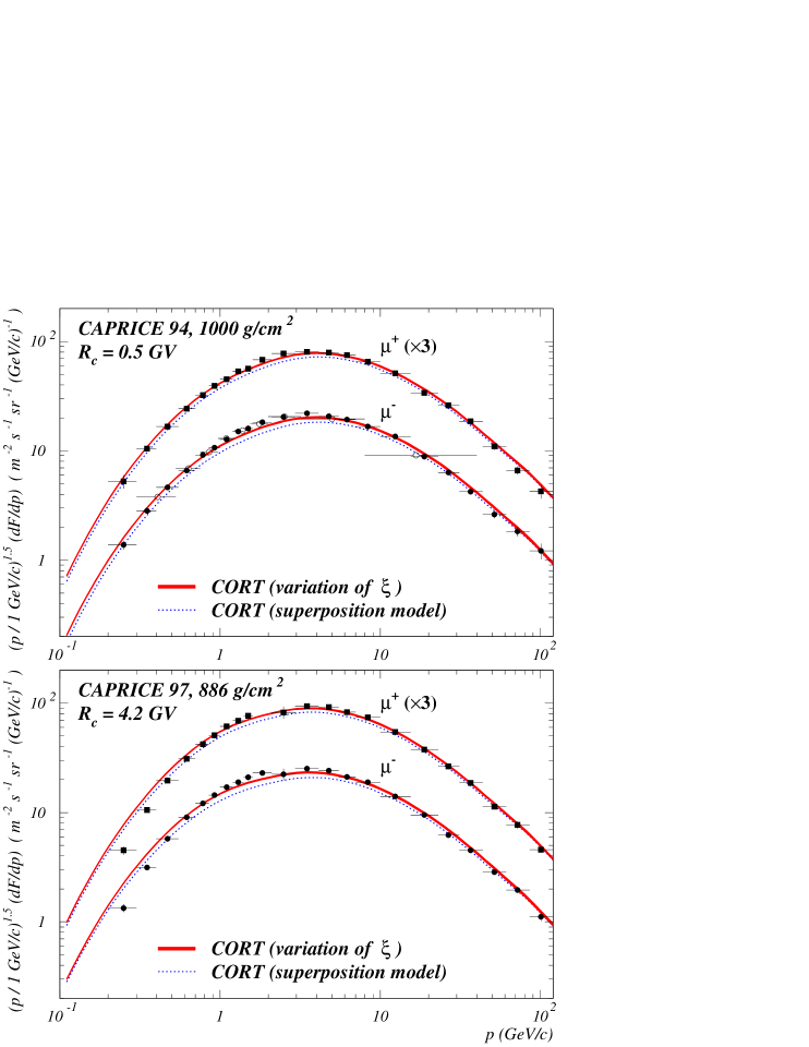
Figure 3: Differential momentum spectra of positive and negative muons at the ground level. The data points are from the experiments CAPRICE 94 [41, 42] and CAPRICE 97 [42]. The curves are calculated with CORT.

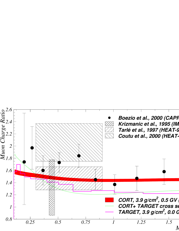
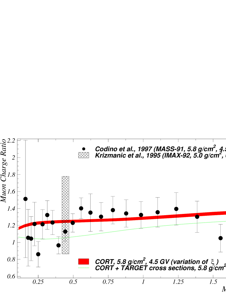
Figure 4: Muon charge ratio near the top of the atmosphere. The points and shaded rectangles represent the data from the experiments MASS 91 [47], IMAX 92 [44], HEAT 95 [45, 46] and CAPRICE 94 [41]. The curves and filled areas are the results of calculations with CORT and TARGET.

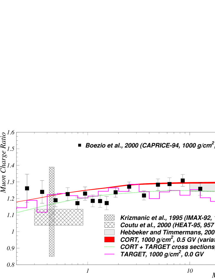
Figure 5: Muon charge ratio at the ground level. The points and shaded rectangles represent the data from the experiments MASS 89 [43], MASS 91 [48], IMAX 92 [44], HEAT 94 [49], HEAT 95 [46], CAPRICE 94 [41] and CAPRICE 97 [42]. The curves and filled areas represent the results of calculations with CORT and TARGET and the best fit obtained in ref. [50] from many experiments at $p\geq 10$ GeV/c.

Several important conclusions can be deduced by comparing the various data presented in figs. 2, 3, 4 and 5.

• There is a substantial agreement between the “standard” CORT predictions and the current muon data within wide ranges of muon momenta and atmospheric depths. In particular, the agreement is good for the region of effective production of leptons, in which the spread of the data (partially related to the procedure of determination of the FAD and mean muon momenta) is minimal. This provides an evidence for the validity of our model.

• The comparison between CORT and CORT+TARGET allows to elucidate the “hadronic” uncertainties in muon fluxes. The only difference between the two calculations is indeed the assumed meson production model and the model for nucleus-nucleus interactions. The $\mu^{-}$ fluxes obtained using the TARGET model systematically exceed the results obtained with our standard model. In order to have a quantitative estimate of the hadronic uncertainties, we note that the muon flux at $p=1$ GeV/c and $h=(100-300)$ g/cm² (i.e. the range where muons and neutrinos are effectively produced) increases by about 50% when the TARGET model is applied. For comparison, we remind that the accuracy of the CAPRICE 94 experiment in this region is about 15%.

• We can see that, except for very small depths, there is a serious disagreement between the CORT+TARGET and the original Bartol results. The disagreement grows fast with decreasing muon momentum and with increasing depth, and it is comparable (or even larger) to the hadronic uncertainties. Since the two calculations are obtained by using the same primary spectrum and the same meson production model, the observed difference can only be due to different features in the nuclear cascade development and muon propagation. On the other hand, the observed agreement at floating altitude, where such features are not important, assures the correctness of our use of the TARGET meson production model. Possible sources for the observed difference could be nucleon elasticity distributions, meson regeneration processes, muon energy losses and some more tiny features of the cascade models under consideration.

6 Numerical results: neutrino fluxes

In this section we present our numerical results for atmospheric neutrino (AN) flux. Due to geomagnetic effects, the AN spectra and angular distributions are quite different for different underground neutrino experiments. However, for the aims of present study it is enough to consider only one representative case. Let us confine ourselves to results pertinent to the Kamioka site.

Figure 6 shows the $\nu_{e}$, $\overline{\nu}_{e}$, $\nu_{\mu}$ and $\overline{\nu}_{\mu}$ energy spectra averaged over all zenith and azimuth angles. The shaded areas are the results obtained with CORT using our standard interaction model. The widths of the areas indicate the uncertainty due to variations of the $\xi$ parameter. One sees that this uncertainty is at most 6% and thus it is negligible. The dashed curves correspond to the CORT+TARGET model, while the circles show the results by a new (preliminary as yet) 3D calculation based on the FLUKA Monte Carlo simulation package [5] (see also [9]). Note that the primary spectrum used in the latter calculation is also a parametrization of the BESS 98 data, which is however not identical to our BESS+JACEE fit. In fig. 7 we compare the zenith-angle distributions of $\nu_{e}$, $\overline{\nu}_{e}$, $\nu_{\mu}$ and $\overline{\nu}_{\mu}$, calculated with CORT (adopting $\xi=0.685$), CORT+TARGET and FLUKA; the distributions are averaged over azimuth angles and over seven energy ranges. The comparison allows to “highlight” the 3D effects which are highly dependent on neutrino energy and direction of arrival.

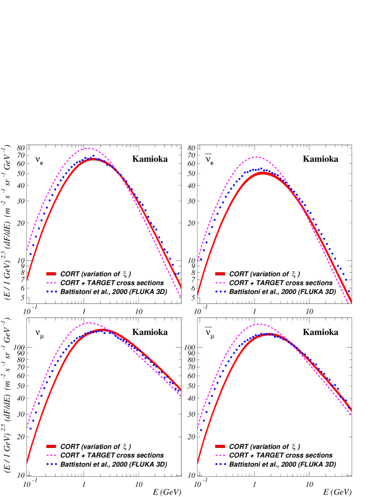
Figure 6: Scaled $4\pi$ averaged fluxes of $\nu_{e}$, $\overline{\nu}_{e}$, $\nu_{\mu}$ and $\overline{\nu}_{\mu}$ for Kamioka site. Shaded areas represent the result of CORT obtained with $\xi$ varying between 0.517 and 0.710. The dashed curves are the result of CORT obtained with the TARGET model for meson production and superposition model for collisions of nuclei. The circles are for the result of a 3D calculation based on the FLUKA code [5].

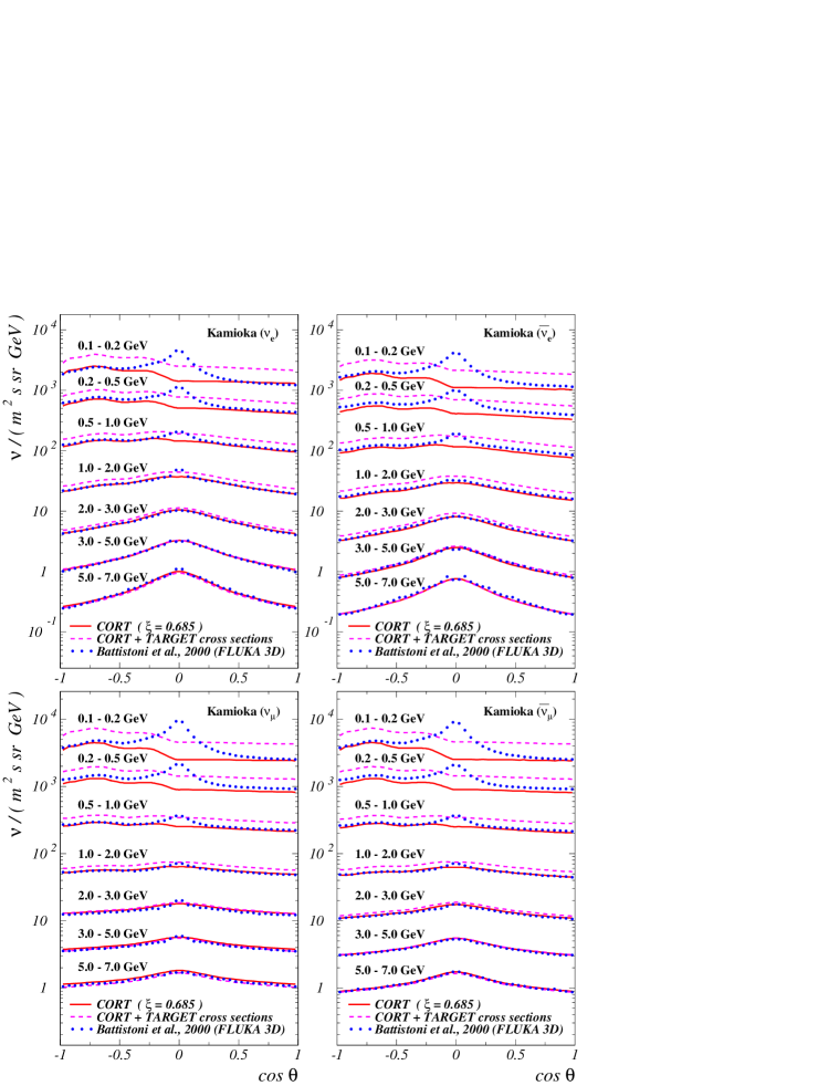
Figure 7: Zenith angle distributions of $\nu_{e}$, $\overline{\nu}_{e}$, $\nu_{\mu}$ and $\overline{\nu}_{\mu}$ for several energy ranges. Solid curves represent the result of CORT obtained with $\xi=0.685$ and the rest notation is the same as in fig. 6.

As a first point, we note that our standard model leads to the lowest AN flux at low energies. Our flux is also essentially lower than that predicted by Bartol group [2] and by Honda et al. [3] and that are used in many analyses of the data from IMB, Fréjus, NUSEX, Kamiokande, Super-Kamiokande, SOUDAN 2 and MACRO.

We do not enter here in the complex problem of the interpretation of the AN anomaly in the light of our result. We want to remark, however, that, in the context of our model, it is difficult to increase the AN flux without spoiling the agreement with the current data on hadronic interactions, primary spectrum and muon fluxes. Let us emphasize that our low AN flux, when it is applied to the analysis of the underground neutrino experiments, results in some electron excess together with (or rather than) the muon deficit in the neutrino induced events.

Table 1: $4\pi$ averaged AN fluxes for Kamioka site calculated with CORT+TARGET and FLUKA and normalized to CORT.

$\Delta E_{\nu}$	CORT+TARGET				FLUKA
(GeV)	$\nu_{e}$	$\overline{\nu}_{e}$	$\nu_{\mu}$	$\overline{\nu}_{\mu}$	$\nu_{e}$	$\overline{\nu}_{e}$	$\nu_{\mu}$	$\overline{\nu}_{\mu}$
0.1–0.2	1.64	1.78	1.72	1.73	1.25	1.45	1.41	1.40
0.2–0.3	1.51	1.68	1.60	1.61	1.23	1.38	1.34	1.33
0.3–0.5	1.42	1.61	1.48	1.50	1.17	1.28	1.22	1.22
0.5–0.7	1.34	1.50	1.36	1.38	1.10	1.19	1.11	1.12
0.7–1.0	1.28	1.41	1.27	1.30	1.05	1.12	1.04	1.05
1.0–2.0	1.20	1.30	1.17	1.20	1.02	1.05	0.99	1.01
2.0–3.0	1.10	1.17	1.03	1.08	0.98	1.03	0.96	0.97
3.0–5.0	1.02	1.07	0.95	1.01	0.99	1.02	0.95	0.97
5.0–7.0	0.95	0.99	0.91	0.96	1.01	1.05	0.94	0.99
7.0–10.	0.91	0.95	0.89	0.93	1.03	1.09	0.95	1.04
10.–20.	0.87	0.91	0.88	0.91	1.07	1.12	0.96	1.02

Let us now discuss in detail the differences between our results and those obtained within CORT+TARGET and FLUKA. The quantitative comparison is given in tables 1 and 2. Table 1 shows the ratios of $4\pi$ averaged AN fluxes, obtained with CORT+TARGET and FLUKA to those with CORT for several energy ranges. In table 2 we tabulate the “flavor ratio”, defined by

$$R_{\nu}=\left(\nu_{e}+\frac{1}{3}\overline{\nu}_{e}\right)\big{/}\left(\nu_{\mu}+\frac{1}{3}\overline{\nu}_{\mu}\right),$$

where $\nu_{e}$, $\overline{\nu}_{e}$, etc. stand for the $4\pi$ averaged fluxes. This quantity is representative for the ratio of $e$ like to $\mu$ like single-ring contained events measured in water Cherenkov detectors and to “showers-to-tracks” ratio measured in iron detectors.

Table 2: Neutrino flavor ratios $R_{\nu}$ calculated with CORT, CORT+TARGET and FLUKA for Kamioka site.

$\Delta E_{\nu}$ (GeV)	CORT	CORT+TARGET	FLUKA
0.1–0.2	0.52	0.51	0.48
0.2–0.3	0.52	0.50	0.49
0.3–0.5	0.51	0.50	0.50
0.5–0.7	0.50	0.50	0.50
0.7–1.0	0.49	0.50	0.50
1.0–2.0	0.47	0.49	0.49
2.0–3.0	0.44	0.47	0.45
3.0–5.0	0.40	0.43	0.42
5.0–7.0	0.36	0.37	0.38
7.0–10.	0.32	0.32	0.34
10.–20.	0.26	0.26	0.29

The comparison between CORT and CORT+TARGET predictions provides a direct determination of the “hadronic” uncertainties in the AN fluxes. We remind indeed that these two results are obtained by using the same primary fluxes and the same code; thus the observed differences is only due to the assumed meson production model. At low energies, the CORT+TARGET predictions drastically exceed those from CORT and even at energies about (2-2.5) GeV one can observe a sizeable difference between the two results. At $E_{\nu}\simeq 0.5$ GeV (tab. 1), the discrepancy is of the order of 40-50%. This shows that the hadronic uncertainties are quite relevant in the energy range which is responsible for the sub-GeV event rate in the Super-Kamiokande detector.

Figs. 6 and 7 show that CORT and FLUKA neutrino fluxes are in good agreement for any zenith angle at energies above $\sim 1$ GeV. On the other hand, CORT is systematically lower than FLUKA for $E_{\nu}\lesssim 1$ GeV. At the energy $E_{\nu}=0.5$ GeV the FLUKA $4\pi$ averaged $\nu_{e}$, $\overline{\nu}_{e}$, $\nu_{\mu}$ and $\overline{\nu}_{\mu}$ fluxes exceed the corresponding CORT results by about 15%, 27%, 18% and 18%, respectively. This discrepancy is only partially due to 3D effects (fig.7), which can account for an increase $\lesssim 10\%$, and it is most probably related to differences between the FLUKA and CORT hadronic interaction models.

Finally, as it is seen from table 2, the flavor ratio is essentially the same in all three models, except for very low energies. As one can conclude from fig. 7, the same is also true for the “up-to-down” asymmetry, that is for the ratio of upward-going ($\cos\theta<0$) and downward-going ($\cos\theta>0$) neutrino fluxes.

7 Conclusions

Let us summarize here the main points of our discussion.

• Calculations with a new version of the 1D code CORT, using the updated KM+SS interaction model and the BESS+JACEE primary spectrum are in agreement with the recent data on muon momentum spectra and charge ratios measured at different atmospheric depths and geomagnetic locations.

• The uncertainty due to indetermination of the parameters of our model for nucleus-nucleus interactions is comparatively small everywhere, except for high altitudes. Some experimental uncertainties (like those due to determination of the flux-weighted average depths) are negligible for the regions of effective generation of leptons and at ground level. Therefore the agreement between the predictions and the muon data obtained at these depths provides a conclusive evidence for validity of our approach.

• Our atmospheric neutrino flux is systematically lower than those used in the current analyses of the data from underground experiments, while the neutrino flavor ratio and “up-to-down” asymmetry are essentially the same as in all recent calculations. We stress that, in the context of our model, it is difficult to increase the AN flux without spoiling the agreement with the current data on hadronic interactions, primary spectrum and muon fluxes.

In order to estimate theoretical uncertainties in the muon and neutrino fluxes we compared our results with those obtained by using different codes and/or interaction models, with the following conclusions.

• By implementing two different interaction models within the same code, we have shown that the “hadronic” uncertainties are quite large at low energies for both muon and neutrino fluxes. Specifically, by using the TARGET meson production model instead of the KM+SS, we obtained a sizeable increase of neutrino fluxes at energies up to $E_{\nu}\simeq 3$ GeV. At the energy $E_{\nu}\simeq 0.5$ GeV representative for the sub-GeV events in the Super-Kamiokande detector, one observes a 40-50% increase of the AN fluxes.

• By comparing two different codes implementing the same interaction model (TARGET), we have shown that other sources of theoretical uncertainties are also relevant. Namely, a sizeable difference exists between the muon fluxes predicted by the original Bartol code and those obtained by implementing the TARGET interaction model within the CORT code. We believe that the observed disagreement is due to the differences in the calculation of nuclear cascade, muon energy loss and decay.

• A comparison of the $4\pi$ averaged AN fluxes calculated with CORT and FLUKA shows rather good agreement at $E_{\nu}>0.7-0.8$ GeV (the difference is typically less than 15%) and a sizable disagreement at lower energies. A comparison of neutrino zenith-angle distributions, predicted by CORT and FLUKA, suggests that the main sources of the disagreement at low energies are the differences in the adopted interaction models and 3D effects.

Finally we conclude that the AN spectra and angular distributions predicted with CORT using the BESS+JACEE primary spectrum and KM-SS interaction model are quite safe at energies above $\sim 1$ GeV while the low-energy range (which is of special importance, as a source of background to the proton decay experiments) is still uncertain.

References

- [1] E. V. Bugaev and V. A. Naumov, Yad. Fiz. 45 (1987) 1380 [Sov. J. Nucl. Phys. 45 (1987) 857]; E. V. Bugaev and V. A. Naumov, Phys. Lett. B 232 (1989) 391.
- [2] G. Barr, T. K. Gaisser and T. Stanev, Phys. Rev. D 39 (1989) 3532; V. Agrawal, T. K. Gaisser, P. Lipari and T. Stanev, Phys. Rev. D 53 (1996) 1314; P. Lipari, T. K. Gaisser and T. Stanev, Phys. Rev. D 58 (1998) 073003.
- [3] M. Honda, K. Kasahara, K. Hidaka and S. Midorikawa, Phys. Lett. B 248 (1990) 193; M. Honda, T. Kajita, K. Kasahara and S. Midorikawa, Phys. Rev. D 52 (1995) 4985; M. Honda, T. Kajita, K. Kasahara and S. Midorikawa, Prog. Theor. Phys. Suppl. 123 (1996) 483.
- [4] H. Lee and Y. S. Koh, Nuovo Cimento B 105 (1990) 883.
- [5] G. Battistoni et al., Nucl. Phys. B (Proc. Suppl.) 70 (1999) 358; G. Battistoni et al., Astropart. Phys. 12 (2000) 315. For the current results see URL http://www.mi.infn.it/battist/neutrino.html
- [6] Y. Tserkovnyak, R. Komar, C. Nally and C. Waltham, preprint hep-ph/9907450.
- [7] T. K. Gaisser et al., Phys. Rev. D 54 (1996) 5578.
- [8] P. Lipari, Astropart. Phys. 14 (2000) 53; P. Lipari, Nucl. Phys. B (Proc. Suppl.) 91 (2000) 159.
- [9] G. Battistoni, Nucl. Phys. B (Proc. Suppl.) 100 (2001) 101.
- [10] V. Plyaskin (for the AMS Collaboration), preprint hep-ph/0103286.
- [11] V. A. Naumov, Investigations on Geomagnetism, Aeronomy and Solar Physics 69 (1984) 82; E. V. Bugaev and V. A. Naumov, INR Reports -0385 and -0401 (1985), unpublished.
- [12] E. V. Bugaev and V. A. Naumov, Izv. Akad. Nauk Ser. Fiz. 50 (1986) 2239 [Bull. Acad. of Sci. of the USSR, Phys. Ser. 50 (1986) 156]; E. V. Bugaev and V. A. Naumov, in: Proc. 2nd Intern. Symposium “Underground Physics’87”, Baksan Valley, August 1987, eds. G. V. Domogatsky et al. (“Nauka”, Moscow, 1988) p. 255; E. V. Bugaev and V. A. Naumov, Yad. Fiz. 51 (1990) 774 [Sov. J. Nucl. Phys. 51 (1990) 493]; E. S. Zaslavskaya and V. A. Naumov, Yad. Fiz. 53 (1991) 477 [Sov. J. Nucl. Phys. 53 (1991) 300]; V. A. Naumov and E. S. Zaslavskaya, Nucl. Phys. B 361 (1991) 675.
- [13] E. V. Bugaev et al., Phys. Rev. D 58 (1998) 054001.
- [14] L. I. Dorman, V. S. Smirnov and M. I. Tiasto, Cosmic rays in the magnetic field of the earth (“Nauka”, Moscow,1971).
- [15] D. F. Smart and M. A. Shea, Adv. Space Res. 14 (1994) 787.
- [16] J. Alcaraz et al., Phys. Lett. B 472 (2000) 215; M. A. Huang, preprint astro-ph/0104229.
- [17] L. I. Dorman, Meteorological effects of cosmic rays (“Nauka”, Moscow, 1972).
- [18] V. A. Naumov, S. I. Sinegovsky and E. V. Bugaev, Yad. Fiz. 57 (1994) 439 [Phys. Atom. Nucl. 57 (1994) 412]; preprint hep-ph/9301263.
- [19] T. Sanuki et al., Astrophys. J. 545 (2000) 1135.
- [20] K. Asakimori et al., Astrophys. J. 502 (1998) 278.
- [21] B. Wiebel-Sooth, P. L. Biermann and H. Meyer, Astron. Astrophys. 330 (1998) 389.
- [22] M. J. Ryan, J. F. Ormes and V. K. Balasubrahmanyan, Phys. Rev. Lett. 28 (1972) 985; 28 (1972) 1497 (Erratum).
- [23] E. S. Seo et al., Astrophys. J. 378 (1991) 763.
- [24] M. Ichimura et al., Phys. Rev. D 48 (1993) 1949.
- [25] J. Buckley J. Dwyer, D. Muller, S. Swordy and K. K. Tang, Astrophys. J. 429 (1994) 736.
- [26] E. Diehl, D. Ellithorpe, D. Müller and S. Swordy, in: Proc. 25th Intern. Cosmic Ray Conf., Durban, South Africa, July 30 – August 6, 1997, eds. M. S. Potgieter et al. (Wesprint, Potchefstroom, Space Research Unit, 1997) vol. 3, p. 405. No result presented in this paper. The data are taken from T. T. von Rosenvinge, ibid., vol. 8, p. 237.
- [27] W. Menn et al., ibid., vol. 3, p. 409.
- [28] F. Aharonian et al., Phys. Rev. D 59 (1999) 092003.
- [29] R. Bellotti et al., Phys. Rev. D 60 (1999) 052002.
- [30] M. Boezio et al., Astrophys. J. 518 (1999) 457.
- [31] J. Alcaraz et al., Phys. Lett. B 490 (2000) 27.
- [32] J. Alcaraz et al., Phys. Lett. B 494 (2000) 193.
- [33] L. R. Kimel’ and N. V. Mokhov, Izv. Vuz. Fiz. 10 (1974) 17; L. R. Kimel’ and N. V. Mokhov, Problems of Dosimetry and Radiation Protection, 14 (1975) 41.
- [34] A. Ya. Serov and B. S. Sychev, Transactions of the Moscow Radio-Engineering Institute, 14 (1973) 173.
- [35] A. N. Kalinovsky, N. V. Mokhov and Yu. P. Nikitin, Transport of high-energy particles through matter (“Energoatomizdat”, Moscow, 1985).
- [36] B. S. Sychev, Cross sections for interactions of high-energy hadrons with atomic nuclei (Moscow Radio-Engineering Institute, Russian Academy of Sciences, 1999).
- [37] V. A. Naumov, in: Proc. Intern. Workshop on Problem in Atmospheric Neutrinos, Gran Sasso, Italy, March 5–6, 1993, eds. V. S. Berezinsky and G. Fiorentini (LNGS, L’Aquila, Italy, 1993), p. 25; V. A. Naumov and T. S. Sinegovskaya, Yad. Fiz. 63 (2000) 2020 [Phys. Atom. Nucl. 63 (2000) 1923].
- [38] A. N. Vall, V. A. Naumov and S. I. Sinegovsky, Yad. Fiz. 44 (1986) 1240 [Sov. J. Nucl. Phys. 44 (1986) 806].
- [39] A. Bialas, M. Bleszyński and W. Czyż, Nucl. Phys. B 111 (1976) 461.
- [40] N. Angelov et al., Yad. Fiz. 30 (1979) 400; E. O. Abdrahmanov et al., Z. Phys. C 5 (1980) 1; M. Kowalski and J. Bartke, Acta Phys. Polon. B 12 (1981) 759.
- [41] M. Boezio et al., Phys. Rev. Lett. 82 (1999) 4757; M. Boezio et al., Phys. Rev. D 62 (2000) 032007.
- [42] J. Kremer et al., Phys. Rev. Lett. 83 (1999) 4241.
- [43] M. P. De Pascale et al., J. Geophys. Res. 98 (1993) 3501.
- [44] J. F. Krizmanic et al., in: Proc. 24th Intern. Cosmic Ray Conf., Rome, Italy, August 28 – September 8, 1995, vol. 1, p. 593.
- [45] G. Tarlé et al., in: Proc. 25th Intern. Cosmic Ray Conf., Durban, South Africa, July 30 - August 6, 1997, eds. M. S. Potgieter et al. (Wesprint, Potchefstroom, Space Research Unit, 1997) vol. 6, p. 321.
- [46] S. Coutu et al., Phys. Rev. D 62 (2000) 032001.
- [47] A. Codino et al., J. Phys. G: Nucl. Part. Phys. 23 (1997) 1751.
- [48] G. Basini et al., in: Proc. 24th Intern. Cosmic Ray Conf., Rome, Italy, August 28 – September 8, 1995 (ARTI Grafiche Editoriali SRL, Urdino, 1995), vol. 1, p. 585.
- [49] E. Schneider et al., ibid., vol. 1, p. 690.
- [50] T. Hebbeker and C. Timmermans, preprint hep-ph/0102042.