Abstract

We calculate the low-energy limit of heavy quark current correlators within an expansion in the inverse heavy quark mass. The induced low-energy currents built from the gluon fields corresponding to the initial heavy quark currents are obtained from an effective action for gauge fields in the one-loop approximation at the leading order of the $1/m$ expansion. Explicit formulae for the low-energy spectra of electromagnetic and tensor heavy quark current correlators are given. Consequences of the appearance of a nonvanishing spectral density below the two-particle threshold for high precision phenomenology of heavy quarks are discussed quantitatively.

1 Introduction

Quantum corrections can qualitatively change the analytic structure of the Green function or the symmetry properties of a classical field-theoretical system. Qualitatively new features compared to the tree level picture may emerge already at finite orders of perturbation theory for Green functions while some effects can only appear as a result of summing up an infinite number of perturbative terms. An effect of non-conservation of the Abelian axial current reveals itself at leading order as a result of the calculation of an one-loop triangle diagram [1, 2] while spontaneous symmetry breaking or bound state formation cannot be observed at any finite order of perturbation theory and requires an infinite summation of relevant subsets of diagrams. For problems related to an investigation of the symmetry properties of quantum systems, such an infinite summation can be readily done by introducing an effective action for the system and calculating it as a loop expansion series. Such an approach reorders the perturbation series with respect to the lines of diagrams related to external fields and allows one to take into account the entire dependence on external fields exactly within a given order of the loop expansion. An effective action can be considered as a generating functional for the vertex (one-particle irreducible, or proper) Green functions (see e.g. Ref. [3]). The treatment of external fields beyond finite order of expansion was done in Ref. [4]. The efficient method of calculating the effective action is based on the Legendre transform of the generating functional for connected Green functions and heavily uses the functional techniques [5]. One can also use a practical calculation technique by substituting the shifted fields in the original Lagrangian of the system [6, 7]. The part of the effective action which is constructed from the constant field is usually called an effective potential and is used to analyze the fundamental symmetry properties of the theory beyond the plain perturbation theory where the effect of the external fields is resummed to all orders. The expansion leading to the effective potential is, in fact, an expansion in Planck’s constant $\hbar$, i.e. the correction accounts for the deflection from the classical limit. Therefore new effects which are absent in the classical approximation may appear within such an approach. An example for this kind of new quantum effects is the light-by-light scattering which emerges as a quantum correction to the photon dynamics due to the interaction with virtual electrons. In the low-energy limit it can be seen as a nonlinearity of the equations for the strong electromagnetic fields in the vacuum. The behaviour of the electromagnetic fields with such a correction can be described by the Euler-Heisenberg Lagrangian [8]. The generalization to non-Abelian fields is discussed in Ref. [9]. The effective potential is also a powerful tool for investigating effects of spontaneous symmetry breaking by quantum corrections [10] and for analyzing the properties of particle systems at finite temperature and density [11].

A special advantage of using the external field technique in gauge theories is an explicit gauge invariance of the effective action that allows to drastically simplify the computation and to reduce the number of necessary diagrams [12]. It is generally believed that in non-Abelian gauge theories the nonperturbative fluctuations (instantons) [13] create a complex vacuum structure that eventually explain (or is responsible for) the low-energy observable spectrum of particles [14]. The technique of calculating in external fields was heavily used for the calculation of quantum corrections to the effective action of gauge fields in the classical instanton background [15]. In practical applications to QCD the complex vacuum structure could explain a phase transition from the quark-gluon representation of Green functions at high energies to the hadron picture at low energies. While the problem of a full description of this transition remains unresolved, Wilson’s operator product expansion which is one of the key tools for calculating the correlation functions at short distances is used for describing hadronic properties at low energies in a semiphenomenological way using sum rule techniques [16]. The external field technique provides a convenient way for practical calculations within the sum rule method based on a semiphenomenological account for the condensates of the local operators [17, 18].

In the present paper we calculate the low-energy limit of heavy quark current correlators within the $1/m$ expansion where $m$ is a heavy quark mass. The induced low-energy currents corresponding to the heavy quark initial operators are obtained from an effective action for gauge fields of the $SU(N_{c})\otimes U(1)$ model in the one-loop approximation at leading order of both the coupling constant and the $1/m$ expansion. Our results for the effective action for vector and tensor currents are presented in Sec. 2. Using the external field technique as a convenient framework for practical calculations of the induced currents in this model, in Sec. 3 we present these induced currents. In Sec. 4 we show phenomenological applications, and in Sec. 5 we deal with the consequences encountered for calculating arbitrary moments.

2 The effective action

While the technique is standard, we are aiming at concrete results for further phenomenological applications to sum rules for the vacuum polarization functions of heavy quarks. Therefore we briefly outline the calculation and the related issues. Further details can be found in Refs. [3, 19]. The Lagrangian of a heavy fermion field $\psi$ interacting with a gauge field ${\cal B}$ of the gauge group $SU(N_{c})\otimes U(1)$ reads

$$L=\bar{\psi}\left(i\gamma^{\mu}\partial_{\mu}+\gamma^{\mu}{\cal B}_{\mu}-m\right)\psi$$ (1)

where ${\cal B}_{\mu}=eA_{\mu}+g_{s}B_{\mu}$. Here $A_{\mu}$ is a gauge field of the $U(1)$ subgroup (photon) with the coupling constant $e$ and $B_{\mu}$ is a gauge field of the $SU(N_{c})$ subgroup (gluon) with the coupling constant $g_{s}$. The matrix notation for the non-Abelian gauge field potentials is used, $B_{\mu}=t_{a}B^{a}_{\mu}$, $t_{a}$ are generators of the gauge group $SU(N_{c})$. A generating functional $W[J]$ of connected Green functions is given by a functional integral with the sources $J$,

$$Z[J] = \exp(iW[J])\ =\ \int[d\bar{\psi}\,d\psi]\exp\left(i\int L^{J}(x)d^{4}x\right)$$ (2)

$$= \int[d\bar{\psi}\,d\psi]\exp\left(i\int\left(\bar{\psi}(i\gamma^{\mu}\partial_{\mu}+\gamma^{\mu}{\cal B}_{\mu}-m)\psi+J^{\mu}{\cal B}_{\mu}\right)d^{4}x\right)$$

where the product $J^{\mu}{\cal B}_{\mu}$ implies a trace with respect to the representation of $SU(N_{c})\otimes U(1)$. A proper gauge fixing is implied as well. The effective action $\Gamma[\bar{\cal B}]$ for the gauge field is then given by the Legendre transform

$$\Gamma[\bar{\cal B}]=W[J]-J\bar{\cal B},\qquad\bar{\cal B}=\frac{\delta W[J]}{\delta J}.$$ (3)

It was shown that this procedure is equivalent to the more direct calculation in external fields (see e.g. Ref. [19]). It is also a generalization of results obtained for constant external fields [2]. Up to leading order in $\hbar$ the effective action constructed with a Legendre transform can also be found through

$$\exp(i\Gamma[{\cal B}])=\int[d\bar{\psi}\,d\psi]\exp\left(i\int\bar{\psi}(i\gamma^{\mu}\partial_{\mu}+\gamma^{\mu}{\cal B}_{\mu}-m)\psi\,d^{4}x\right)=\det\left(i\gamma^{\mu}\partial_{\mu}+\gamma^{\mu}{\cal B}_{\mu}-m\right)$$ (4)

where ${\cal B}$ is now a classical gauge field (integration over $d^{4}x$ is implied for expressions of the action). By using the identity $\det M=\exp({\rm tr}(\ln M))$ for an operator $M$ one continues with

$$i\Gamma[{\cal B}]={\rm tr}\Big{[}\ln\left(i\gamma^{\mu}\partial_{\mu}+\gamma^{\mu}{\cal B}_{\mu}-m\right)\Big{]}.$$ (5)

2.1 Results for the effective action

A straightforward calculation of the functional determinant gives a correction to the effective low-energy action of the gauge fields within $SU(N_{c})\otimes U(1)$. We calculate the leading nontrivial contribution in the $1/m$ expansion. The functional determinant in loop expansion can be represented by Feynman diagrams. A diagram which gives a correction to the effective action due to a heavy quark loop is shown in Fig. 1.

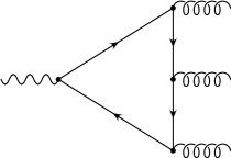
Figure 1: Heavy quark loop correction to the electromagnetic current

Two-gluon transitions are forbidden according to a generalization of Farry’s theorem to non-Abelian theories [20]. We are interested in the behaviour of the amplitude associated with the diagram in Fig. 1 at low energies and, therefore, take the limit of a very heavy quark. Formally the limit $m\to\infty$ is taken which in physical terms means that $m$ is much larger than all momenta of external legs of the diagram in Fig. 1, namely the three gluons and the photon. A straightforward calculation of the diagram presented in Fig. 1 gives the one-loop result for the correction to the effective action induced by a heavy quark loop at leading order of the $1/m$ expansion. It reads

$$\Delta\Gamma_{\rm QCD}=\frac{eg_{s}^{3}d_{abc}}{180m^{4}(4\pi)^{2}}\Big{[}14{\rm tr}(FG^{a}G^{b}G^{c})-5{\rm tr}(FG^{a}){\rm tr}(G^{b}G^{c})\Big{]}$$ (6)

where $F_{\mu\nu}$ is a field strength tensor for the $U(1)$ subgroup, $G_{\mu\nu}=t_{a}G^{a}_{\mu\nu}$ is the field strength tensor for the $SU(N_{c})$ subgroup, and $d_{abc}$ are the totally symmetric $SU(N_{c})$ structure constants defined by the relation $d_{abc}=2{\rm tr}(\{t_{a},t_{b}\}t_{c})$. The trace in Eq. (6) is understood as a trace with respect to the Lorentz indices of the fields, i.e. one considers the strength tensors of gauge fields as matrices for which ${\rm tr}(FG^{a})=F^{\mu\nu}G^{a}_{\nu\mu}$. This makes the formulae shorter and more transparent. Before we proceed to the calculation of the induced current in the next section, we compare the result with the corresponding expression in QED.

2.2 Comparison with QED

The effective action within QED corresponding to Eq. (6) is known as Euler-Heisenberg Lagrangian [19],

$$\Delta\Gamma_{\rm QED}=\frac{2\alpha^{2}}{45m^{4}}\Big{[}(\vec{E}^{2}-\vec{H}^{2})^{2}+7(\vec{E}\cdot\vec{H})^{2}\Big{]},\qquad\alpha=\frac{e^{2}}{4\pi}$$ (7)

which can be obtained from Eq. (6) by replacing $d_{abc}$ by $1$ and $G^{a}_{\mu\nu}$ by $F_{\mu\nu}$, supplemented by the obvious substitution $g_{s}\to e$. Using the definitions for the electric field $\vec{E}$ and the magnetic field $\vec{H}$,

$$F^{0j}=-F_{0j}=-E_{j},\quad F^{i0}=-F_{i0}=E_{i},\quad F^{ij}=F_{ij}=-\epsilon_{ijk}H_{k}$$ (8)

one finds

$${\rm tr}(F^{2})=2(\vec{E}^{2}-\vec{H}^{2}), {\rm tr}(F^{4})=2(\vec{E}^{2}-\vec{H}^{2})^{2}+4(\vec{E}\cdot\vec{H})^{2},$$

$${\rm tr}(F\tilde{F})=4(\vec{E}\cdot\vec{H}), {\rm tr}(F\tilde{F}F\tilde{F})=-\frac{1}{2}({\rm tr}(F^{2}))^{2}+{\rm tr}(F^{4})=4(\vec{E}\cdot\vec{H})^{2}$$ (9)

where

$$\tilde{F}_{\mu\nu}=\frac{1}{2}\epsilon_{\mu\nu\rho\sigma}F^{\rho\sigma}.$$ (10)

Note for further use and convenience that in order to rewrite the expressions from one form to another there is one more relation between the fourth-order monomials of the electromagnetic field strength tensor $F_{\mu\nu}$,

$$(F\tilde{F})^{2}=-2(F^{2})^{2}+4F^{4}$$ (11)

with

$$F\tilde{F}=F^{\mu\nu}\tilde{F}_{\mu\nu},\qquad F^{2}=F^{\mu\nu}F_{\mu\nu},\qquad F^{4}=F^{\mu\nu}F_{\nu\alpha}F^{\alpha\beta}F_{\beta\mu}.$$ (12)

Therefore the correspondence between Eq. (6) and its QED counterpart in Eq. (7) is established.

3 The induced current

An expression for the induced electromagnetic current $J^{\mu}$ as being an effective electromagnetic current for the low-energy effective theory describing the interaction of photons and gluons is given by the derivative of the effective action with respect to the external Abelian gauge field,

$$eJ^{\mu}=-\frac{\delta\Gamma[{\cal B}]}{\delta A_{\mu}}=-{\rm tr}\left[ie\gamma_{\mu}\,\frac{1}{i\gamma^{\mu^{\prime}}\partial_{\mu^{\prime}}+\gamma^{\mu^{\prime}}{\cal B}_{\mu^{\prime}}-m}\right].$$ (13)

The derivative with respect to $A_{\mu}$ can be replaced by a derivative with respect to $F_{\mu\nu}=\partial_{\mu}A_{\nu}-\partial_{\nu}A_{\mu}$,

$$eJ^{\mu}(x)=-\frac{\delta F_{\mu^{\prime}\nu^{\prime}}}{\delta A_{\mu}}\ \frac{\delta\Gamma[{\cal B}]}{\delta F_{\mu^{\prime}\nu^{\prime}}}=-2\partial_{\nu}\frac{\delta\Gamma[{\cal B}]}{\delta F_{\nu\mu}}.$$ (14)

3.1 Results for the induced vector current

With the explicit expression for the effective action given in Eq. (6) we obtain [21]

$$J^{\mu}=\partial_{\nu}{\cal O}^{\mu\nu},\qquad{\cal O}^{\mu\nu}=\frac{-g_{s}^{3}d_{abc}}{90m^{4}(4\pi)^{2}}[14(G^{a}G^{b}G^{c})^{\mu\nu}-5(G^{a})^{\mu\nu}{\rm tr}(G^{b}G^{c})].$$ (15)

Note that the current conservation $\partial_{\nu}J^{\mu\nu}=0$ is automatically guaranteed because the operator ${\cal O}^{\mu\nu}$ is antisymmetric, ${\cal O}^{\mu\nu}+{\cal O}^{\nu\mu}=0$. Higher order corrections in the coupling constant $\alpha$ of the $U(1)$ subgroup are omitted. The induced electromagnetic current in Eq. (15) is a correction of order $1/m^{4}$ in the inverse heavy quark mass which vanishes in the limit of an infinitely heavy quark. Corrections in the inverse heavy quark masses are important for tests of the standard model at the present level of precision and have been already discussed in various areas of particle phenomenology [22, 23, 24].

3.2 Other types of induced currents

Expressions for the induced currents with quantum numbers other than that of the electromagnetic current $J^{PC}=1^{--}$ can be obtained in a similar way. The axial current of fermions naturally appears in the standard model as a result of an axial-vector interaction of fermions with $W$ and $Z$ bosons. The corresponding induced current can be obtained as a derivative of the respective effective action with respect to the $Z$ boson field. The leading order diagram, however, contains only two external legs and is UV divergent. In case of massless fermions this diagram leads to the anomalous non-conservation of the axial current that also requires a strict definition of the corresponding operator $\bar{\psi}\gamma_{\mu}\gamma_{5}\psi$ within perturbation theory because its renormalization is not dictated by the Ward identities any more. The leading corrections to the anomaly of the axial current for massless fermions due to strong interactions were considered in Refs. [25, 26] where implications of the Adler-Bardeen no-go theorem (non-renormalizability) were discussed also for dimensional regularization and different definitions of the axial current at the tree level. Higher order corrections were analyzed in Ref. [27]. Explicit high order corrections to the expression for the anomaly depend on the renormalization prescription for the composite operator $\bar{\psi}\gamma_{\mu}\gamma_{5}\psi$ within perturbation theory.

The scalar current $\bar{\psi}\psi$ appears in an interaction vertex for the Higgs boson and was intensively studied. The decay $H\to\gamma\gamma$ is described by the effective interaction

$$\Delta L_{H}=g_{S}\alpha HFF$$ (16)

with the parameter $g_{S}$ (remark the different to $g_{s}$, $S$ stands for the scalar current) given by the corresponding one-loop diagram with two external photons. Here $H$ is an interpolating field for the Higgs boson. The decay of the Higgs boson into two photons is calculated up to high orders of perturbation theory and mass expansion [28]. The application of the effective potential technique to the analysis of the correlators of the scalar gluonic currents which emerge in the decay of the Higgs boson into hadrons was considered in Ref. [29].

3.3 Results for the induced tensor current

In the context of the effective action we consider a tensor current of the form

$$J^{\mu\nu}=\bar{\psi}\sigma^{\mu\nu}\psi,\qquad\sigma^{\mu\nu}=\frac{i}{2}[\gamma^{\mu},\gamma^{\nu}]$$ (17)

and calculate its low-energy limit induced by a heavy quark loop. The properties of this current are rather similar to those of the electromagnetic current. Note that the classical vector mesons ($\rho$, $\omega$, $\phi$) interact with this current and can be produced by it. We introduce an interaction

$$\Delta L_{T}=g_{T}\bar{\psi}\sigma^{\mu\nu}\psi F_{\mu\nu}$$ (18)

in the Lagrangian of heavy quarks and readily find the effective action for gauge fields induced by such a vertex. The low-energy limit at the one-loop order reads

$$\Gamma_{T}=\frac{-g_{T}g_{s}^{3}d_{abc}}{180m^{3}(4\pi)^{2}}\left(32{\rm tr}(FG^{a}G^{b}G^{c})-15{\rm tr}(FG^{a}){\rm tr}(G^{b}G^{c})\right)$$ (19)

with the same notations as in Eq. (6). According to the form of the effective interaction in Eq. (18) the induced current $J_{\mu\nu}$ is given by a derivative

$$g_{T}J^{\mu\nu}=-\frac{\delta\Gamma_{T}}{\delta F_{\mu\nu}}$$ (20)

and explicitly reads

$$J^{\mu\nu}=\frac{-g_{s}^{3}d_{abc}}{180m^{3}(4\pi)^{2}}\left(32(G^{a}G^{b}G^{c})^{\mu\nu}-15(G^{a})^{\mu\nu}{\rm tr}(G^{b}G^{c})\right).$$ (21)

Note the lower power of the heavy quark mass in Eq. (21) as compared to Eq. (15).

4 Phenomenological applications

High precision tests of the standard model remain one of the main topics of particle phenomenology [30]. The recent observation of a possible signal from the Higgs boson may complete the experimentally confirmed list of the standard model particles [31]. Because experimental data are becoming more and more accurate, the determination of numerical values of the parameters of the standard model Lagrangian will require more accurate theoretical formulae. Recently an essential development in high-order perturbation theory calculations has been observed. A remarkable progress has been made in the heavy quark physics where a number of new physical effects have been described theoretically with high precision. The cross section of top–antitop production near the threshold has been calculated at the next-to-next-to-leading order of an expansion in the strong coupling constant and velocity of a heavy quark with an exact account for Coulomb interaction (as a review, see Refs. [32, 33]). This theoretical breakthrough allows for the best determination of a numerical value of the top quark mass from experimental data. The method of Coulomb resummation resides on a nonrelativistic approximation for the Green function of the quark-antiquark system near the threshold and has been successfully used for the heavy quark mass determination within sum rule techniques [34, 35, 36]. Being applied to quarkonium systems this method is considered to give the best estimates of heavy quark mass parameters [37, 38, 39, 40]. Technically an enhancement of near-threshold contributions to sum rules is achieved by considering integrals of the spectral density of the heavy quark production with weight functions which suppress the high-energy tail of the spectrum. The integrals with weight functions $1/s^{n}$ for different positive integer $n$, $s=E^{2}$, where $E$ is the total energy of the quark-antiquark system, are called moments of the spectral density and are most often used in the sum rule analysis [41]. The interest in the precision determination of the $c$-quark mass is especially high because this parameter introduces the largest uncertainty to the theoretical calculation of the running electromagnetic coupling constant at $M_{Z}$ which is one of the key quantities for the constraints to the Higgs boson mass [42]. We stress that in the corresponding determination of the running electromagnetic coupling constant at $M_{Z}$ based on direct integration of experimental data over the threshold region, the sensitivity of the results to the $c$-quark mass is much weaker [43].

For phenomenological applications of our results one therefore has to compute the two-point correlation functions of induced currents. In the following we show that there is a strong constraint on the order $n$ of the moment that can be used in heavy quark sum rules. Because of the contribution of low-energy gluons, only the first few moments exist if the theoretical expressions for the correlators include the $O(\alpha_{s}^{3})$ order of perturbation theory.

4.1 The spectrum for the induced vector current correlator

First we discuss the case of the vector current where the data are obtained from $e^{+}e^{-}$ annihilation experiments and are rather precise. The basic quantity for the analysis of a vector current $j^{\mu}=\bar{q}\gamma^{\mu}q$ of a heavy fermion $q$ within sum rules is the vacuum polarization function

$$12\pi^{2}i\int\langle Tj_{\mu}(x)j_{\nu}(0)\rangle e^{iqx}d^{4}x=(q_{\mu}q_{\nu}-g_{\mu\nu}q^{2})\Pi(q^{2}).$$ (22)

With the spectral density $\rho(s)$ defined by the relation

$$\rho(s)=\frac{1}{2\pi i}(\Pi(s+i0)-\Pi(s-i0)),\quad s>0,$$ (23)

the dispersion representation

$$\Pi(q^{2})=\int\frac{\rho(s)ds}{s-q^{2}}$$ (24)

holds. A necessary regularization and subtraction is assumed in Eq. (24). The normalization of the vacuum polarization function $\Pi(q^{2})$ in Eq. (22) is chosen such that one obtains the high-energy limit $\lim_{s\to\infty}\rho(s)=1$ for a lepton. For the quark in the fundamental representation of the gauge group $SU(N_{c})$ the high-energy limit of the spectral density reads $\rho(\infty)=N_{c}$. The integral in Eq. (24) runs over the whole spectrum of the correlator in Eq. (22) or over the whole support of the spectral density $\rho(s)$ in Eq. (23).

A correlator of the induced vector current $J^{\mu}$ has the general form

$$\langle TJ^{\mu}(x)J^{\nu}(0)\rangle=-\partial_{\alpha}\partial_{\beta}\langle T{\cal O}^{\mu\alpha}(x){\cal O}^{\nu\beta}\rangle$$ (25)

where an explicit expression of the current as a derivative of the antisymmetric operator ${\cal O}^{\mu\nu}$ has been employed. The resulting correlator $\langle T{\cal O}^{\mu\alpha}(x){\cal O}^{\nu\beta}\rangle$ in Eq. (25) contains only gluonic operators. Such correlators were considered previously in the framework of perturbation theory [44, 45]. In leading order of perturbation theory the correlator in Eq. (25) has a topological structure of a sunset diagram, as it is shown in Fig. 2(a).

Figure 2: Induced massless correlator diagrams

Technically, a convenient procedure of computing the sunset-type diagrams is to work in configuration space [46]. We find

$$\langle TJ_{\mu}(x)J_{\nu}(0)\rangle=\frac{-34d_{abc}d_{abc}}{2025\pi^{4}m^{8}}\left(\frac{\alpha_{s}}{\pi}\right)^{3}\left(\partial_{\mu}\partial_{\nu}-g_{\mu\nu}\partial^{2}\right)\frac{1}{x^{12}}.$$ (26)

A Fourier transform of the correlator in Eq. (26) gives the vacuum polarization function in momentum space which reads

$$12\pi^{2}i\int\langle TJ_{\mu}(x)J_{\nu}(0)\rangle e^{iqx}d^{4}x=(q_{\mu}q_{\nu}-g_{\mu\nu}q^{2})\Pi(q^{2})$$ (27)

where at small $q^{2}$ ($q^{2}\ll m^{2}$)

$$\Pi(q^{2})|_{q^{2}\approx 0}=C_{g}\left(\frac{q^{2}}{4m^{2}}\right)^{4}\ln\left(\frac{\mu^{2}}{-q^{2}}\right),\qquad C_{g}=\frac{17d_{abc}d_{abc}}{243000}\left(\frac{\alpha_{s}}{\pi}\right)^{3}.$$ (28)

For QCD with the colour group $SU(3)$ one has $d_{abc}d_{abc}=40/3$. The spectral density of the vacuum polarization function $\Pi(q^{2})$ in Eq. (27) is given at small values for $s$ by

$$\rho(s)|_{s\approx 0}=C_{g}\left(\frac{s}{4m^{2}}\right)^{4}.$$ (29)

Note that the spectral density in Eq. (29) can be found without an explicit calculation of its Fourier transform. Instead one can use a spectral decomposition (dispersion representation) in configuration space which was heavily employed for the analysis of sunset diagrams in Ref. [46]. In this particular instance the spectral representation of the correlator in configuration space reads

$$\frac{i}{x^{12}}=\frac{\pi^{2}}{2^{8}\Gamma(6)\Gamma(5)}\int_{0}^{\infty}s^{4}D(x^{2},s)ds$$ (30)

with $D(x^{2},s)$ being the propagator of a scalar particle of mass $\sqrt{s}$,

$$D(x^{2},m^{2})=\frac{im\sqrt{-x^{2}}K_{1}(m\sqrt{-x^{2}})}{4\pi^{2}(-x^{2})}$$ (31)

where $K_{1}(z)$ is the McDonald function (a modified Bessel function of the third kind, see e.g. Ref. [47]). $\Gamma(z)$ is Euler’s gamma function.

An asymptotic behaviour of the spectral density of the corresponding contribution for large energies (where the limit of massless quarks can be used) enters the expression for the ratio $R(s)$ of $e^{+}e^{-}$ annihilation into hadrons and has been known since long ago [48, 49, 50]. This term is usually called light-by-light (lbl) contribution and reads

$$R^{\rm lbl}(s)=\left(\frac{\alpha_{s}}{\pi}\right)^{3}\frac{d_{abc}d_{abc}}{1024}\left(\frac{176}{3}-128\zeta(3)\right).$$ (32)

Here $\zeta(z)$ is the Riemann $\zeta$ function with $\zeta(3)=1.20206\ldots$ The contribution to the spectral density given in Eq. (32) is negative while our result given in Eq. (29) is positive as it should be the case for the spectral density of the electromagnetic current as a Hermitean operator.

4.2 The spectrum for the induced tensor current correlator

The results for the correlator of the tensor current given in Eq. (21) are slightly more complicated. The correlator reads

$$12\pi^{2}i\int\langle Tj_{\mu\nu}(x)j_{\alpha\beta}(0)\rangle e^{iqx}d^{4}x\ =\ (g_{\mu\alpha}g_{\nu\beta}-g_{\mu\beta}g_{\nu\alpha})\Pi_{g}(q^{2})$$ (33)

$$+(g_{\mu\alpha}q_{\nu}q_{\beta}-g_{\mu\beta}q_{\nu}q_{\alpha}-g_{\nu\alpha}q_{\mu}q_{\beta}+g_{\nu\beta}q_{\mu}q_{\alpha})\Pi_{q}(q^{2})$$

where two scalar amplitudes are possible now. One finds

$$\Pi_{g}(q^{2})=-\frac{q^{2}}{2}\Pi_{q}(q^{2})=\frac{61d_{abc}d_{abc}}{729000}\left(\frac{\alpha_{s}}{\pi}\right)^{3}\frac{-q^{2}}{4}\left(\frac{q^{2}}{4m^{2}}\right)^{3}\ln\left(\frac{\mu^{2}}{-q^{2}}\right).$$ (34)

The physical content of the amplitudes $\Pi_{g}(q^{2})$ and $\Pi_{q}(q^{2})$ is related to contributions of the states with $J^{PC}=1^{--}$ and $J^{PC}=1^{+-}$, resp. Note that the sum rule analysis for the mesons with quantum numbers $J^{PC}=1^{+-}$ has been done in Ref. [51] with quark interpolating currents. From the present results we also see a possibility to use gluonic currents as interpolating operators for such mesons. The validity of such a description depends strongly on the strength of the interaction of the meson in question with the corresponding interpolating operator which is difficult to estimate independently.

Note that there are only two independent gluonic operators to construct the induced currents under consideration. The electromagnetic current is given by a derivative of a special linear combination of these operators while the tensor current is given by a linear combination of operators themselves. There is one more current relevant to the situation. It originates from the Gordon decomposition of the electromagnetic current (see e.g. Ref. [19])

$$2m\bar{\psi}\gamma^{\mu}\psi=\partial_{\nu}(\bar{\psi}\sigma^{\mu\nu}\psi)+\bar{\psi}\ i\!\!\buildrel\leftrightarrow\over{D}\!{}^{\mu}\psi.$$ (35)

This relation retains for the induced currents as well. The left hand side and the right hand side of Eq. (35) have different parity as for the number of Dirac $\gamma$-matrices between spinor fields which is reflected in an additional factor $m$ at the left hand side of Eq. (35). In the massless limit these types of currents are alien and can never mix. At the level of induced currents the Dirac structure of the initial heavy quark currents is reflected in different degrees of suppression by the heavy quark mass $m$.

4.3 The spectrum for a mixed current correlator

Having both currents at hand, one can study a mixed correlator of the form

$$12\pi^{2}i\int\langle TJ_{\mu}(x)J_{\alpha\beta}(0)\rangle e^{iqx}d^{4}x=i(g_{\mu\alpha}q_{\beta}-g_{\mu\beta}q_{\alpha})\Pi_{M}(q^{2})$$ (36)

with a single scalar amplitude $\Pi_{M}(q^{2})$. Such mixed correlators are useful in sum rule applications [52]. One finds

$$\Pi_{M}(q^{2})=\frac{67d_{abc}d_{abc}}{972000}\left(\frac{\alpha_{s}}{\pi}\right)^{3}\frac{-q^{2}}{4m}\left(\frac{q^{2}}{4m^{2}}\right)^{3}\ln\left(\frac{\mu^{2}}{-q^{2}}\right)$$ (37)

The physical content of the amplitude is given by the $J^{PC}=1^{--}$ resonance, i.e. by the $\Upsilon$-family in case of $b$ quarks.

5 Moments of the spectral density

As mentioned earlier, the moments of the spectral density $\rho(s)$ of the form

$${\cal M}_{n}=\int\frac{\rho(s)ds}{s^{n+1}}$$ (38)

are usually studied within the sum rule method for heavy quarks [41]. These moments are related to the derivatives of the vacuum polarization function $\Pi(q^{2})$ at the origin,

$${\cal M}_{n}=\frac{1}{n!}\left(\frac{d}{dq^{2}}\right)^{n}\Pi(q^{2})\bigg{|}_{q^{2}=0}.$$ (39)

Such moments are chosen in order to suppress the high energy part of the spectral density $\rho(s)$ which is not measured accurately in the experiment. Within the sum rule method one assumes that the moments in Eq. (38) can be calculated for any $n$ or, equivalently, that the derivatives in Eq. (39) exist for any $n$. The existence of moments seems to be obvious because one implicitly assumes that the spectral density $\rho(s)$ of the heavy quark electromagnetic currents vanishes below the two-particle threshold $s=4m^{2}$ which means that the vacuum polarization function $\Pi(q^{2})$ of heavy quarks is analytic in the whole complex plane of $q^{2}$ except for the cut along the positive real axis starting from $4m^{2}$. This assumption about the analytic properties of the vacuum polarization function $\Pi(q^{2})$ is known to be wrong if a resummation of Coulomb effects to all orders of perturbation theory is performed: as a result of such a resummation the Coulomb bound states appear below the perturbation theory threshold $s=4m^{2}$.

5.1 Infrared singular behaviour of the moments

The qualitatively new feature of effective currents given in Eqs. (15) and (21) is that they are expressed through massless fields. Therefore the spectrum of the two-point correlators of these currents start at zero energy. This feature drastically changes the analytic structure of the two-point correlators of these currents and, in particular, their infrared (IR) or small $s$ behaviour because of the branching point (cut) singularity of $\Pi(q^{2})$ at the origin $q^{2}=0$. This new feature of having a nonvanishing spectrum below the formal tree-level two-particle threshold which appears at the $O(\alpha_{s}^{3})$ order of perturbation theory for induced current correlators has important phenomenological consequences. Indeed, such a change of the analytic structure of induced current correlators affects strongly the theoretical expressions for some observables usually employed in heavy quark physics for the precision determination of the parameters of heavy quarks and their interactions.

Because of the low-energy gluon contributions, the large $n$ moments of the spectral density in Eq. (38) do not exist and cannot be used for phenomenological analyses. Caused by the factor $(s/4m^{2})^{4}$ in Eq. (38) the moments become IR singular for $n\geq 4$ in case of the induced vector current. This can already be seen by looking at the factor $1/m^{4}$ in the induced vector current in Eq. (15). For the induced tensor current the corresponding moments start to diverge earlier because of a weaker suppression by the heavy quark mass, the corresponding factor in Eq. (21) is $1/m^{3}$ instead of $1/m^{4}$. Therefore, in this case the moments become IR singular already for $n\geq 3$. Note that in early considerations of sum rules quite large $n$ were used. For instance, the numerical value of the gluon condensate was extracted from sum rules for the moments with $n\sim 10\div 20$ [41, 53]. In view of our result on the low-energy behaviour of the spectral density, one has either to limit the accuracy of theoretical calculations for the moments to the $O(\alpha_{s}^{2})$ order of perturbation theory which seems insufficient for a high precision analysis of quarkonium systems (especially if the Coulomb resummation to all orders is performed) or to use only a few first moments. For small $n$, however, the high-energy contribution, which is not known experimentally with a reasonable precision, is not sufficiently suppressed and introduces a large quantitative uncertainty into the sum rules for the moments. An analysis based on finite energy sum rules is free from such a problem and can be used in phenomenological applications [54].

Note in passing that there is no low-energy gluon contribution (and therefore no low-energy divergence problem) for correlators of the currents containing only one heavy quark with mass $m$. The spectrum of such correlators starts at $m^{2}$ and there are no massless intermediate states contributing to the correlator in perturbation theory (see e.g. Ref. [55]). The theoretical expressions for such correlators can be used for high precision tests of theoretical predictions when the accuracy of experimental data in corresponding channels will improve in the future.

5.2 An infrared safe moment definition

The infinite-integration sum rules with large $n$ can be retained at high orders of perturbation theory if an appropriate cutoff at small energies is introduced. This can be readily achieved by calculating the moments (or derivatives) at some Euclidean point $q^{2}=-\Delta$ [56]. Indeed, for the regularized moments

$${\cal M}_{n}(\Delta)=\frac{1}{n!}\left(\frac{d}{dq^{2}}\right)^{n}\Pi(q^{2})\bigg{|}_{q^{2}=-\Delta}=\int\frac{\rho(s)ds}{(s+\Delta)^{n+1}}$$ (40)

there is no divergence at small $s$. However, the regularization parameter $\Delta$ cannot be arbitrary small. The reason is that the resulting correlator of gluonic currents in Eq. (25) is essentially normalized at $\mu^{2}=\Delta$ when radiative corrections are taken into account, like the diagram shown in Fig. 2(b). The corrections are known to be large and, therefore, $\Delta$ is much larger than the expected IR scale in quark channels [44]. This observation makes the phenomenological analysis based on the regularized sum rules in Eq. (40) unprecise even for reasonably large $n$ because the continuum contribution to moments is not suppressed for large values of $\Delta$. The suppression of the high-energy tail can be enhanced by constructing a more special kind of moments which exploit the explicit behaviour of the spectral density at low energy. The IR safe moments with a more efficient suppression of high-energy tail for the induced vector current have the form

$${\tilde{\cal M}}_{n}(\Delta)=\int\frac{\rho(s)ds}{s^{3}(s+\Delta)^{n+1}}$$ (41)

It seems that even in such an optimized form these moments cannot be used for the $c\bar{c}$-system, i.e. for analyzing $J/\psi$ resonances because the suppression is insufficient for achieving the precision goals necessary for the $c$-quark mass determination. For the $b\bar{b}$-system, i.e. for the analysis of $\Upsilon$-resonances the dependence on the cutoff $\Delta$ is numerically essential for moments at large $n$ and for $\Delta$ as large as $\Delta=1\div 2{\rm\,GeV}^{2}$ which is still small according to the estimates of radiative corrections in gluonic channels. We would like to remind the reader that Coulomb poles which are essential for the analysis of the $\Upsilon$-resonance and $b\bar{b}$-production near threshold give contributions which are formally of the $O(\alpha_{s}^{3})$ order (for the value of the Coulombic wave function at the origin see e.g. Ref. [37]), an order which coincides with the order of corrections considered here (see Eq. (28)). The theoretical expressions for the correlators in the scalar channel where below threshold corrections start at the $O(\alpha_{s}^{2})$ order are more sensitive to these special below threshold contributions. However, data in the scalar channel are considerably worse than those in the vector channel and there is no possibility of a high precision analysis on the scalar channel at present.

6 Conclusions

We have presented corrections to the heavy quark currents induced by a virtual heavy quark loop and expressed through the gluon operators. We have considered the electromagnetic current and the tensor current closely related to it. Heavy quark loop induced corrections first appear at $O(\alpha_{s}^{3})$ order of perturbation theory and are given by the $1/m^{4}$ term of the mass expansion in case of the electromagnetic current and by the $1/m^{3}$ term in case of the tensor current. The spectra of the correlators of such induced currents start at zero energy. This fact makes impossible the standard analysis of the moment sum rules at $O(\alpha_{s}^{3})$ order of perturbation theory for $n\geq 4$ in case of the electromagnetic current and for $n\geq 3$ in case of the tensor current.

Acknowledgements

The work is partially supported by the Russian Fund for Basic Research under contracts 99-01-00091 and 01-02-16171. A.A. Pivovarov is an Alexander von Humboldt fellow. S. Groote acknowledges a grant given by the Deutsche Forschungsgemeinschaft, Germany.

References

- [1] S.L. Adler, Phys. Rev. 177 (1969) 2426; J.S. Bell and R. Jackiw, Nuovo Cim. A60 (1969) 47; R. Jackiw and K. Johnson, Phys. Rev. 182 (1969) 1459; S.L. Adler and W.A. Bardeen, Phys. Rev. 182 (1969) 1517;
- [2] J. Schwinger, Phys. Rev. 82 (1951) 664.
-
[3]
N.N. Bogoliubov and D.V. Shirkov,
“Introduction to the theory of quantized fields,” Wiley, New York, 1980 -
[4]
G. Jona-Lasinio, Nuovo Cim. 34 (1964) 1790;
J. Goldstone, A. Salam and S. Weinberg, Phys. Rev. 127 (1962) 965 - [5] J. Iliopoulos, C. Itzykson and A. Martin, Rev. Mod. Phys. 47 (1975) 165
- [6] R. Jackiw, Phys. Rev. D9 (1974) 1686
- [7] S.Y. Lee and A.M. Sciaccaluga, Nucl. Phys. B96 (1975) 435
- [8] W. Heisenberg and H. Euler, Z. Phys. 98 (1936) 714
- [9] S.G. Matinian and G.K. Savvidy, Nucl. Phys. B134 (1978) 539
- [10] S. Coleman and E. Weinberg, Phys. Rev. D7 (1973) 1888
- [11] A.D. Linde, Phys. Rev. D14 (1976) 3345
-
[12]
B.S. de Witt, Phys. Rev. 162 (1967) 1195, 1239;
L.F. Abbott, Nucl. Phys. B185 (1981) 189 - [13] A.A. Belavin, A.M. Polyakov, A.S. Shvarts and Yu.S. Tyupkin, Phys. Lett. B59 (1975) 85
- [14] C.G. Callan, R.F. Dashen and D.J. Gross, Phys. Lett. B63 (1976) 334
- [15] G. ’t Hooft, Phys. Rev. D14 (1976) 3432; Erratum ibid. D18 (1978) 2199
- [16] K.G. Wilson, Phys. Rev. 179 (1969) 1499
- [17] M.A. Shifman, A.I. Vainshtein and V.I. Zakharov, Nucl. Phys. B147 (1979) 385
- [18] V.A. Novikov et al., Fortschr. Phys. 32 (1984) 585
- [19] C. Itzykson and J.B. Zuber, “Quantum Field Theory,” McGraw-Hill, New York, 1980
- [20] N.V. Smolyakov, Theor. Math. Phys. 50 (1982) 225
- [21] S. Groote and A.A. Pivovarov, “Low-energy gluon contributions to the vacuum polarization of heavy quarks,” Report No. MZ-TH/01-06 [hep-ph/0103047]
- [22] A.A. Pivovarov, JETP Lett. 53 (1991) 536, Phys. Lett. B263 (1991) 282; A.A. Penin and A.A. Pivovarov, Phys. Rev. D49 (1994) 265; Phys. Part. Nucl. 29 (1998) 286
- [23] K.G. Chetyrkin, Phys. Lett. B307 (1993) 169
- [24] S.A. Larin, T. van Ritbergen and J.A. Vermaseren, Nucl. Phys. B438 (1995) 278
-
[25]
G.T. Gabadadze and A.A. Pivovarov,
JETP Lett. 54 (1991) 298;
Phys. Atom. Nucl. 56 (1993) 565; J. Math. Phys. 35 (1994) 1045 - [26] M. Bos, Nucl. Phys. B404 (1993) 215
- [27] S.A. Larin, Phys. Lett. B303 (1993) 113
- [28] K.G. Chetyrkin, B.A. Kniehl, M. Steinhauser and W.A. Bardeen, Nucl. Phys. B535 (1998) 3; K.G. Chetyrkin, B.A. Kniehl and M. Steinhauser, Phys. Rev. Lett. 79 (1997) 353; Nucl. Phys. B490 (1997) 19
- [29] N.V. Krasnikov and A.A. Pivovarov, Phys. Lett. B161 (1995) 373
- [30] D.E. Groom et al., Eur. Phys. J. C15 (2000) 1
-
[31]
R. Barate et al. [ALEPH Collaboration],
Phys. Lett. B495 (2000) 1;
M. Acciarri et al. [L3 Collaboration], Phys. Lett. B495 (2000) 18 - [32] A.H. Hoang et al., Eur. Phys. J. direct C3 (2000) 1
- [33] A.A. Penin and A.A. Pivovarov, “Analytical results for and cross sections near the threshold up to the next-to-next-to-leading order of NRQCD,” Report No. MZ-TH/98-61 [hep-ph/9904278]; A.A. Pivovarov, “ cross section near the production threshold in NNLO of NRQCD,” Report No. MZ-TH/99-65 [hep-ph/0009036]
- [34] M.B. Voloshin, Nucl. Phys. B154 (1979) 365
- [35] H. Leutwyler, Phys. Lett. B98 (1981) 447
-
[36]
M.B. Voloshin, Int. J. Mod. Phys. A10 (1995) 2865;
M.B. Voloshin and Y.M. Zaitsev, Sov. Phys. Usp. 30 (1987) 553 - [37] J.H. Kühn, A.A. Penin and A.A. Pivovarov, Nucl. Phys. B534 (1998) 356; A.A. Penin and A.A. Pivovarov, Phys. Lett. B435 (1998) 413; Nucl. Phys. B549 (1999) 217
- [38] K. Melnikov and A. Yelkhovsky, Phys. Rev. D59 (1999) 114009
- [39] A. Hoang and T. Teubner, Phys. Rev. D60 (1999) 114027
- [40] T. Nagano, A. Ota and Y. Sumino, Phys. Rev. D60 (1999) 114014
- [41] V.A. Novikov et al., Phys. Rept. 41 C (1978) 1
- [42] A.A. Pivovarov, “Running electromagnetic coupling constant: low-energy normalization and the value at ,” Report No. MZ-TH/00-51 [hep-ph/0011135]
-
[43]
J.H. Kühn and M. Steinhauser,
Phys. Lett. B437 (1998) 425;
M. Davier, A. Höcker, Phys. Lett. B435 (1998) 427;
S. Groote, J.G. Körner, K. Schilcher and N.F. Nasrallah, Phys. Lett. B440 (1998) 375 -
[44]
A.L. Kataev, N.V. Krasnikov and A.A. Pivovarov,
Phys. Lett. B107 (1981) 115;
Nucl. Phys. B198 (1982) 508; Erratum, Nucl. Phys. B490 (1997) 505;
A.A. Pivovarov, Yad. Fiz. 63 (2000) 1646 - [45] T. Inami, T. Kubota and Y. Okada, Z. Phys. C18 (1983) 69
-
[46]
S. Groote, J.G. Körner and A.A. Pivovarov,
Phys. Lett. B443 (1998) 269;
Nucl. Phys. B542 (1999) 515; Eur. Phys. J. C11 (1999) 279;
S. Narison and A.A. Pivovarov, Phys. Lett. B327 (1994) 341 - [47] G.N. Watson, “Theory of Bessel functions,” Cambridge Univ. Press, Cambridge, 1944
- [48] S.G. Gorishnii, A.L. Kataev and S.A. Larin, Phys. Lett. B259 (1991) 144
- [49] K.G. Chetyrkin, Phys. Lett. B391 (1997) 402
- [50] L.R. Surguladze and M.A. Samuel, Phys. Rev. Lett. 66 (1991) 560; Erratum ibid p. 2416
-
[51]
A.A. Ovchinnikov and A.A. Pivovarov,
Nuovo Cim. A90 (1985) 73;
Sov. J. Nucl. Phys. 43 (1986) 1006; Yad. Fiz. 43 (1986) 1564 -
[52]
V.A. Novikov, M.A. Shifman, A.I. Vainshtein, M.B. Voloshin
and V.I. Zakharov,
Nucl. Phys. B237 (1984) 525 - [53] S.N. Nikolaev and A.V. Radyushkin, Phys. Lett. B124 (1983) 243
-
[54]
N.V. Krasnikov and A.A. Pivovarov,
Phys. Lett. B112 (1982) 397;
N.V. Krasnikov, A.A. Pivovarov and A.N. Tavkhelidze, Z. Phys. C19 (1983) 301 -
[55]
S. Groote, J.G. Körner and A.A. Pivovarov,
“Analytical calculation of heavy baryon correlators in NLO of perturbative
QCD,” to be published in the Proceedings of 7th International Workshop on
Advanced Computing and Analysis Techniques in Physics Research (ACAT 2000),
Batavia, Illinois, 16-20 Oct 2000, Report No. MZ-TH/00-41 [hep-ph/0009218];
S. Groote, J.G. Körner and A.A. Pivovarov,
Phys. Rev. D61 (2000) 071501;
A.A. Pivovarov, “High order perturbative calculations for heavy quarks near threshold,” Report No. MZ-TH/00-40 [hep-ph/0009107] - [56] L.J. Reinders, H. Rubinstein and S. Yazaki, Phys. Rept. 127 (1985) 1