IPPP/01/13

DCPT/01/26

27 March 2001

Summary Talk:

First Workshop on Forward Physics and

Luminosity Determination at the LHC

A.D. Martin^a

^a Department of Physics and Institute for Particle Physics Phenomenology, University of Durham, Durham, DH1 3LE

An attempt is made to summarize the discussion at the Workshop, except for the panel discussion on the ability of the LHC detectors to accommodate forward reactions. The Workshop focused on two main topics. The first topic was forward physics at the LHC. Predictions were made for forward reactions, including elastic scattering and ‘soft’ diffractive processes, in terms of (multi) Pomeron exchange, using knowledge gained at lower energies. The survival probability of rapidity gaps accompanying hard subprocesses was studied. The nature of the Pomeron, before and after QCD, was exposed, and some aspects of small $x$ physics at the LHC were considered. The second topic of the Workshop concerned the accuracy of the luminosity measuring processes at the LHC. Attention concentrated on three methods. The classic approach based on the optical theorem, secondly, the observation of the pure QED process of lepton-pair ($\ell^{+}\ell^{-}$) production by photon-photon fusion and, finally, the measurement of inclusive $W$ and $Z$ production.

1 Introduction

A lot of effort has justifiably been spent on the central detectors of the LHC experiments so that ‘hard’ interactions can be triggered on, and observed, in order to expose New Physics. However the vast majority of interactions are ‘soft’ with particles predominantly going forward, and the physics of this domain is one of the subjects of the Workshop. The relevant processes, forward elastic scattering and ‘soft’ diffraction, are driven by Pomeron (or rather by multi-Pomeron) exchange. They are interesting in their own right, although in the period after the advent of QCD they did not attract so much attention. However in the last few years the situation has changed. A stimulus came from the observation of diffractive processes at HERA and the Tevatron, characterised by the presence of rapidity gaps. Moreover, diffractive processes have been proposed as possible ways to identify New Physics. For example, the central production of a Higgs boson with a rapidity gap on either side is advocated as a possible discovery channel at the LHC. The chance that these gaps survive the soft rescattering of the colliding hadrons was one of the topics of discussion.

The second subject of the Workshop was the way to measure the luminosity of the LHC. Three methods were discussed:

• the classic method based on the optical theorem,

  $$\left.\frac{d\sigma_{\rm el}}{dt}\right|_{t=0}\;=\;\frac{\sigma_{\rm tot}^{2}}{16\pi}\>(1+\rho^{2}),$$ (1)

  where $\rho$ is the ratio of the real to the imaginary part of the forward elastic amplitude (Coulomb effects have been neglected in (1)),

• to measure pure QED $e^{+}e^{-}$ or $\mu^{+}\mu^{-}$ production via photon-photon fusion

  $$pp\;\rightarrow\;p\>+\>\ell^{+}\ell^{-}\>+\>p,$$ (2)

• to measure inclusive $W$ or $Z$ production.

At first sight it might appear that an accurate measurement of the luminosity is not essential. However, for example, precision measurements in the Higgs sector of accuracy of about 7% require the uncertainty in the measurement of the luminosity to be 5% or less [2]. At this Workshop, Tapprogge [3] summarised the physics reasons why a precise measurement of the luminosity of the LHC is important.

2 Proposed forward $pp$ measurements

Bozzo [4] presented the TOTEM experimental programme, which will take place in the very first runs at the LHC. The plan is to measure $\sigma_{\rm tot}$ by a luminosity-independent method

$$\sigma_{\rm tot}\;=\;\frac{16\pi}{(1+\rho^{2})}\;\frac{(dN_{\rm el}/dt)_{t=0}}{N_{\rm el}+N_{\rm inel}},$$ (3)

with an absolute error of about 1 mb. The TOTEM inelastic detector will be installed inside the CMS experiment, with the elastic scattering “roman pot” detectors located at distances in the interval 100 to 200 m from the crossing point. The TOTEM measurements need special runs at the ‘low’ initial luminosity, with high $\beta^{*}$ optics for an accurate measurement of the small scattering angles. The detector should be efficient to within 2 mm of the beam and can reach down to about $-t=0.01~{}{\rm GeV}^{2}$. They will collect about 100 events/sec for $-t<1~{}{\rm GeV}^{2}$ at a luminosity ${\cal L}=10^{28}~{}{\rm cm}^{-2}~{}{\rm s}^{-1}$. The differential cross section will also be measured in the interval $1<|t|<10~{}{\rm GeV}^{2}$ in the high luminosity runs. TOTEM also plans an inclusive trigger for the measurement of single diffraction.

We also heard at the Workshop about the novel microstation concept for forward measurements [5]. The microstation is a light, compact device which could be integrated with the beam pipe. It could be used in situations where there are severe space and mass limitations for the inelastic detector, such as in the ATLAS experiment. The elastic proton measurement would be like that for TOTEM, so again it should be possible to reach down to $-t\sim 0.01~{}{\rm GeV}^{2}$.

Piotrzkowski [6] considered the possibility of using the LHC as a $\gamma\gamma$ collider, and noted how the present TOTEM layout may be modified to allow the tagging of protons with small energy losses. In principle, this would allow the study of $\gamma\gamma\rightarrow H$ etc. in a broad region of $\gamma\gamma$ centre-of-mass energy about 200 GeV, with an effective $\gamma\gamma$ luminosity that is reduced by about $10^{-3}$–$10^{-2}$ of that of the LHC.

Guryn [7] presented the PP2PP experimental physics programme at RHIC. Their main goal is to make a detailed study of the spin dependence of the proton-proton interaction in the kinematic range

$$50\;<\;\sqrt{s}\;<\;500~{}{\rm GeV}\quad\quad\quad{\rm and}\quad\quad\quad 4\;\times\;10^{-4}\;<\;|t|\;<\;1.5~{}{\rm GeV}^{2},$$ (4)

in order to probe features of the Pomeron. At the beginning they will measure $d\sigma_{\rm el}/dt$ down to $-t=0.006~{}{\rm GeV}^{2}$, and study the $t$ dependence of the slope. Later they will explore the Coulomb-nuclear interference region, and determine $\rho$. By measuring the spin asymmetries $A_{N},A_{NN},A_{LL}$ they will obtain information on the five independent $pp\rightarrow pp$ helicity amplitudes.

Block [8] discussed the determination of $\sigma_{\rm tot}(pp)$ at $\sqrt{s}\simeq 30$ TeV from cosmic ray data. He emphasized the importance of the relation between the slope $B$ of the elastic scattering distribution and $\sigma_{\rm tot}$ for energies well above the accelerator regime, and the reliance on a model of proton-air interactions.

3 Extrapolation of $d\sigma_{\rm el}/dt$ to $t=0$

Vorobyov [9] reminded us how at ISR energies, and below, it was possible to make precision measurements of the elastic differential cross section at small momentum transfer down into the Coulomb-nuclear interference region. From these experiments one could make a determination of the local slope

$$B(t)\;=\;\frac{d\ln(d\sigma_{\rm el}/dt)}{dt}$$ (5)

as a function of $t$, measure the ratio $\rho$ of the real to imaginary part of the forward amplitude and reliably determine the total cross section from the optical point. However the application of this method becomes more and more difficult as we go up to Tevatron and then LHC energies, due to the decrease of the typical scattering angle and the inability to experimentally reach the Coulomb-nuclear interference region.

Figure 1: ISR data for $pp\;d\sigma_{\rm el}/dt$, with the experimental exponential form divided out, compared with the description given by a multi-Pomeron analysis [10]. The Coulomb-nuclear interference is evident in the data at very small $t$. The dashed curve should be disregarded, as it shows the prediction with high-mass diffraction neglected. The continuous and dotted curves are obtained using two extremum models for high-mass diffraction.

Figure 2: As for Fig. 1 but showing $Sp\bar{p}S$ elastic data. The most recent UA4 data are unnormalised and are plotted higher for clarity.

Figure 3: As for Fig. 1 but showing Tevatron elastic data.

Figs. 1, 2 and 3 show data at ISR, CERN $Sp\bar{p}S$ and Tevatron energies respectively. In the first two plots we see the Coulomb interference spike at very small $t$, whereas at the Tevatron the spike is no longer accessible and the data of the two experiments extrapolate to different values at $t=0$. Moreover at the ISR we see, from Fig. 1, a change of the local slope with $t$,

$$B(0)\>-\>B(|t|=0.2~{}{\rm GeV}^{2})\;\simeq\;2~{}{\rm GeV}^{-2},$$ (6)

whereas at the Tevatron the data suggest less variation for $|t|\lower 3.01385pt\hbox{$\;\stackrel{{\scriptstyle\textstyle<}}{{\sim}}\;$}0.4~{}{\rm GeV}^{2}$, see Fig. 3. A global description of these and other forward data gives the $t$ dependence of the local slopes shown in Fig. 4 [10]. The dashed curves should be ignored as they come from a description which does not include high-mass diffraction. The remaining two curves (continuous and dotted) are obtained using two extremum models for high-mass diffraction, and give a measure of the level of the theoretical ambiguity in $B(t)$. The predictions at the LHC energy mean that we should be able to extrapolate the TOTEM measurements to $t=0$ with an error of less than 0.5% coming from the variation of the local slope. Even if the cross section were measured only in the interval $0.05<|t|<0.15~{}{\rm GeV}^{2}$, then the uncertainty at $t=0$ would be less than 3% due to the variation of $B(t)$.

Figure 4: The multi-Pomeron model [10] predictions for the $t$-dependence of the local elastic slope, $B(t)$ of (5), at ISR, $Sp\bar{p}S$, Tevatron and LHC energies. The rise of the dashed curve is due to the diffractive minimum, which is considerably modified by the inclusion of high-mass diffraction, as shown by the continuous and dotted curves.

4 The Pomeron and the description of forward data

High energy $pp$ scattering at small momentum transfer $t$ is driven by Pomeron $t$-channel exchange. In fact we were reminded at the Workshop [11, 12] how in 1960, Gribov startled the community by showing that the behaviour of the $pp$ amplitude

$$A(s,t)\;=\;isf(t),$$ (7)

which gives the asymptotic behaviour

$$\sigma_{\rm tot}\;=\;{\rm constant},\quad\quad\sigma(pp)\;=\;\sigma(p\bar{p}),$$ (8)

contradicts $t$-channel unitarity. Gribov noted that a possible solution was to introduce the Regge behaviour

$$A(s,t)\;=\;is^{\alpha_{I\!\!P}(t)}\>f(t),$$ (9)

with a Pomeron trajectory $\alpha_{I\!\!P}(t)=\alpha_{I\!\!P}(0)+\alpha^{\prime}t$, with intercept $\alpha_{I\!\!P}(0)=1$ and slope $\alpha^{\prime}>0$. This is in agreement with $t$-channel unitarity, while still giving relations (8). In addition to the Pomeron pole, there are also Regge cuts coming from multiple Pomeron exchange, which led to the development of Gribov’s Reggeon calculus, involving renormalisation of the bare pole, Mandelstam crossed diagrams [13], AGK cutting rules [14], etc. This ‘soft’ Pomeron was the subject of the talks by Landshoff [15] and Kaidalov [16].

Landshoff [15] showed that a good description of the available data for high energy $\sigma_{\rm tot}$ and $d\sigma_{\rm el}/dt$ at small momentum transfer is given by a simple effective Pomeron pole trajectory

$$\alpha_{\rm eff}(t)\;=\;1.08\>+\>\alpha^{\prime}t$$ (10)

with $\alpha^{\prime}=0.25~{}{\rm GeV}^{-2}$. This is a remarkable simplification, but of course it is necessarily incomplete for the reasons that are mentioned below.

Figure 5: The Pomeron exchange contribution (a), together with unitarity corrections (b–e). Note that graphs (d, e) are the ‘square’ of the single- and double-diffractive dissociation amplitudes respectively — and that their constituent Pomeron lines are subjected to rescattering corrections.

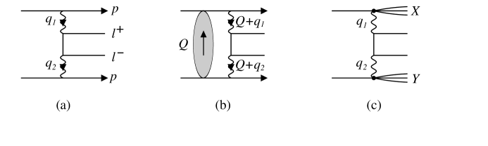
Kaidalov [16] explained that to describe phenomena in the forward region, it is important to extend single-Pomeron exchange so as to explicitly include the multi-Pomeron effects. At very high energy such effects are needed to restore $s$-channel unitarity, but, as we will see in a moment, they are also necessary at current energies. Fig. 5 shows examples of typical corrections to the bare Pomeron pole of diagram (a). First, iterations of the pole amplitude via elastic unitarity gives contributions of the type shown in diagram (b). If we take into account the possibility of proton excitations $(p\rightarrow N^{*})$ in intermediate states, then we must include contributions such as that in diagram (c). These iterations are implemented in terms of a two-channel eikonal formalism [17, 18]. Note that diagrams (b) and (c) are very symbolic — by implication they incorporate the Mandelstam crossed diagrams [13] and satisfy the AGK cutting rules [14]. The second $(N^{*})$ channel effectively allows for low mass diffractive dissociation. The excitation into high mass $(M_{X})$ states is described by the triple-Pomeron graph (d) for single-diffractive dissociation (with cross section $\sigma_{\rm SD}$), and by (e) for double-diffractive dissociation $(\sigma_{\rm DD})$. To be self-consistent, the Pomeron lines in (d) and (e) actually represent the final Pomeron amplitude with all the screening effects included. In addition to (d), there is an equal contribution $\sigma_{\rm SD}$ from dissociation of the lower proton only. The contribution of graphs of the type (b)–(e) are not negligible. Indeed, using the AGK rules, it may be estimated that the correction to (a) is

$$\sigma_{D}/\sigma_{\rm tot}\;\equiv\;(\sigma_{\rm el}\>+\>2\sigma_{\rm SD}\>+\>\sigma_{\rm DD})/\sigma_{\rm tot}\>\sim\>0.4$$ (11)

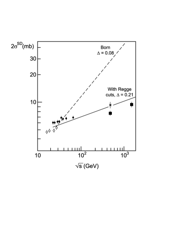
at the LHC. A most convincing way to see the necessity of multi-Pomeron rescattering effects at current energies is to look at the energy behaviour of $\sigma_{\rm SD}$. If only the bare Pomeron is used, as in diagram (d), then the cross section grows as

$$\sigma_{\rm SD}\;\sim\;s^{2\alpha_{I\!\!P}(t)-2},$$ (12)

whereas when rescattering effects are included

$$\sigma_{\rm SD}\;\sim\;\sigma_{\rm tot}/\ln s.$$ (13)

The difference is dramatic, as Fig. 6 shows. The physical origin of this result is that the high energy proton-proton interaction reaches the black-disc limit for central values of the impact parameter, and forces inelastic diffraction to come from the peripheral region with $b\sim c\ln s$.

Figure 6: The energy behaviour of the cross section for single-diffractive dissociation compared to the predictions of the effective pole and multi-Pomeron approaches [16]. $\Delta\equiv\alpha(0)-1$.

A related observation was made by Schlein [19]. He showed that the single diffractive data in the ISR-Tevatron energy range can be described by the triple-Regge formula, provided that the effective intercept $\alpha_{I\!\!P}(0)$ decreased with increasing $s$. Such an $s$ dependent behaviour of the effective intercept may be interpreted as a manifestation of the multi-Pomeron exchange effects.The bare Pomeron, together with the multi-Pomeron corrections, should give a global description of all forward phenomena, including $\sigma_{\rm tot},d\sigma_{\rm el}/dt,\rho,\sigma_{\rm SD},\sigma_{\rm DD}$ and $\langle n_{\rm ch}\rangle$. Several analyses have been undertaken at various levels of sophistication to all or parts of the data. Recent examples are given in [10, 20, 21]. Perhaps the most complete study to date is that of Ref. [10], which is in the spirit of the much earlier pioneering work of Kaidalov et al. [22]. It describes the forward phenomena in high energy $pp$ (and $p\bar{p}$) collisions using a multi-Pomeron approach which embodies:

• pion-loop insertions in the bare Pomeron pole, which represent the nearest singularity generated by $t$-channel unitarity,

• a two-channel eikonal which incorporates the Pomeron cuts generated by elastic and quasi-elastic (with $N^{*}$ intermediate states) $s$-channel unitarity.

• high mass single and double diffractive dissociation.

The resulting description of $d\sigma_{\rm el}/dt$ data is shown in Figs. 1–3 and the corresponding $t$ dependence of the local slope $B(t)$ is given in Fig. 4. Surprisingly, the bare Pomeron pole parameters turn out to be

$$\Delta\;\equiv\;\alpha(0)\>-\>1\;\simeq\;0.10,\quad\quad\alpha^{\prime}\;=\;0,$$ (14)

which is to be contrasted to those of the effective pole (10). Thus the shrinkage of the diffraction cone comes not from the bare pole, but rather has components from the three ingredients, (i)–(iii), of the model. That is, in the ISR-Tevatron energy range [23]

$${\rm``}\alpha_{\rm eff}^{\prime}"\;=\;(0.034\>+\>0.15\>+\>0.066)~{}{\rm GeV}^{-2}$$ (15)

from the $\pi$-loop, $s$-channel eikonalization and diffractive dissociation respectively. We saw [9] that at lower energies the fixed target data require $\alpha_{\rm eff}^{\prime}=0.14~{}{\rm GeV}^{-2}$, which is consistent with (15) since as the energy decreases the effect of the eikonal and higher mass diffractive dissociation reduces. Moreover eikonal rescattering suppresses the growth of the cross section with $\sqrt{s}$, so to describe the same data we require $\Delta>\Delta_{\rm eff}\simeq 0.08$.

Figure 7: The energy behaviour of the $pp$ forward elastic slope and the total cross section of the multi-Pomeron approach [10], compared with that obtained from the simple effective pole form of (10). $\sigma_{\rm tot}$ is plotted in fm² and $B(0)$ in GeV^-2, since in these units the asymptotic black-disc limit takes, to a good approximation, the simple form $B(0)/\sigma_{\rm tot}\rightarrow 1$. The figure is taken from Ref. [23].

Another observable difference between the naive effective pole and the multi-Pomeron approach is in the energy behaviour of the slope $B(0)$. This is illustrated in Fig. 7, together with the behaviour of $\sigma_{\rm tot}$. It is seen that, while the two approaches give similar values of $\sigma_{\rm tot}$ up to LHC energies, the predictions for the slope $B(0)$ at the LHC already differ significantly.

In Table 1 we show some predictions for the forward observables at the LHC. Note that the BH predictions [20] are based on a single-channel eikonal, and do not therefore involve inelastic diffraction. The KMR prediction is an update of [10].

	KPT [22]	KMR [10]	BH [20]
	1986	2000	2000
$\sigma_{\rm tot}$ (mb)	103	108	107
$2\sigma_{\rm SD}$ (mb)	12	15	-
$\sigma_{\rm DD}$ (mb)	13	8	-
$B(0)$ (GeV-2)	21.5	20.7	19.4
$\rho=$ Re/Im	0.11	0.11	0.11
$\sigma_{\rm el}$ (mb)	26		31

Table 1: Predictions for forward observables at the LHC.

5 Hard diffraction and gap survival probabilities

There is much interest in the survival probability of rapidity gaps which feature in the various hard diffractive and other high energy processes. The rapidity gaps, which naturally occur whenever we have colour-singlet $t$-channel exchange [24, 1, 25], tend to get populated by secondary particles from the soft rescattering processes. A multi-Pomeron analysis incorporates rescattering in some detail and so allows the calculation of the survival probabilities $S^{2}$ of the gaps. Recently attention has focused on the size of $S^{2}$, see for example [26, 10, 20, 27, 28], because of the possibility of extracting New Physics from hard processes, accompanied by gaps, in an almost background-free environment and, from a theoretical viewpoint, because of its reliance on subtle QCD techniques. The theoretical calculations of $S^{2}$ do not allow for the practical difficulties of isolating rapidity gap processes in the ‘pile-up’ events which may occur at high LHC luminosity.

To calculate $S^{2}$, it is convenient to work in impact parameter space. Let ${\cal M}(s,b)$ be the amplitude of the particular hard process of interest at centre-of-mass energy $\sqrt{s}$. Then the probability that there is no extra inelastic interaction is

$$S^{2}\;=\;\frac{\int\>|{\cal M}|^{2}\>e^{-\Omega}\>d^{2}b}{\int\>|{\cal M}|^{2}\>d^{2}b},$$ (16)

where $\Omega(s,b)$ is the opacity (or optical density) of the interaction of the incoming protons. For simplicity we show the formula with the simple one-channel eikonal. In practice the numerator and denominator in (16) are sums over the diffractive eigenstates, each with their own characteristic opacity $\Omega_{i}$. The opacities $\Omega_{i}(s,b)$ reach a maximum at the centre of the proton and become small in the periphery. Clearly the survival probability $S^{2}$ depends strongly on the spatial distribution of the constituents of the relevant subprocess, and on the dynamics of the whole diffractive part of the scattering matrix. Contrary to frequent claims in the literature, it is important to note that $S^{2}$ is not universal, but depends on the particular hard subprocess, as well as the kinematical configurations. In particular, $S^{2}$ depends on the nature of the colour-singlet exchange (Pomeron or, possibly, $W/Z$ or photon exchange) which generates the gap [10], as well as on the characteristic momentum fractions carried by the active partons in the colliding hadrons [35]. This leads to a rich structure of the probability of rapidity gaps in processes mediated by colour-singlet $t$-channel exchange. The framework was introduced long ago [29, 30], but only with the advent of rapidity gap events being observed in hard processes at the Tevatron and at HERA, is this rich physics now revealing itself. Clearly it is important to have reliable estimates of the survival probabilities so as to be able to predict the rate for rapidity gap processes at the LHC. Indeed, the possibility of using central Higgs production with a rapidity gap either side as a discovery channel at the LHC was discussed at the Workshop by Khoze [27].

Examples of estimates of the survival probability for single- and double-diffractive dissociation (SD, DD), and central diffraction (CD) are given in Table 2. By central diffraction we mean a centrally produced state $X$ with rapidity gaps on either side. The $b$ dependence of the various diffractive processes is

$$|{\cal M}|^{2}\;\propto\;\exp(-b^{2}/nB^{\prime}),$$ (17)

where $n=3,4$ and 2 for SD, DD and CD respectively and $B^{\prime}$ is the slope of the diffractive inclusive cross section [10]. The single channel eikonal model of [20] gives values of $S^{2}$, very similar to those of the DD column.

$\sqrt{s}$	$B^{\prime}$	survival probability $S^{2}$ for:
(TeV)	(GeV-2)	SD	DD	CD
1.8	4.0	0.10	0.15	0.05
	5.5	0.15	0.21	0.08
14	4.0	0.06	0.10	0.02
	5.5	0.09	0.15	0.04

Table 2: The survival probability $S^{2}$ of rapidity gaps in single, double and central diffractive processes at Tevatron and LHC energies [10].

Figure 8: The partonic structure of (a) diffractive dijet production at the Tevatron and (b) diffractive deep inelastic scattering at HERA. Process (a) has soft rescattering corrections (not shown) which give secondaries which populate the rapidity gap associated with Pomeron exchange, and hence suppress the cross section.

An experimental manifestation of the survival probability $S^{2}$ comes from comparing hard diffraction at the Tevatron with that observed at HERA. The relevant plot was presented by Snow [32], see also [33]. It shows the recent CDF measurements of diffractive dijet production as a function of $\beta$, together with the expectations based on convoluting the parton densities of the Pomeron (and those of the proton) with the partonic-level cross sections of the hard subprocess. $\beta$ is the momentum fraction of the Pomeron entering the hard subprocess. The parton densities of the Pomeron are determined from diffractive deep-inelastic-scattering data at HERA [34]. The partonic structure of the Tevatron dijet production and HERA diffractive DIS are sketched in Fig. 8. However, as the CDF plot [33, 32] shows, when the HERA Pomeron densities are used to estimate Tevatron dijet production, the factorized prediction turns out to be about an order of magnitude larger than the data. A key assumption of the factorization estimate is that the survival probability of the rapidity gap, associated with the Pomeron exchange, is the same in Figs. 8(a) and 8(b). Comparison of the diagrams shows that the breakdown of factorization is an inevitable consequence of QCD, and occurs naturally, due to the small probability $S^{2}$ for the rapidity gap to survive the soft rescattering which occurs between the incoming hadrons at the Tevatron, but which is absent between the electron and the proton at HERA. In fact, a detailed study of this comparison, including the $\beta$ dependence, tells us about the dependence of the survival probability on the kinematic variables [35], and opens the door to the application to many other hard processes with rapidity gaps, including those discussed by Khoze [27].

6 The QCD Pomeron and small $x$ physics

Lipatov gave a comprehensive survey of the Pomeron before and after QCD [11]. Since he was either close to, or pioneered, all these developments, it was a masterly and informative summary. The Pomeron before QCD was the subject of Section 4. That Pomeron was a Reggeon, even if it has a rather unusual Regge trajectory, which in the time-like ($t>0$) region is mixed with the $f$ and $f^{\prime}$ meson trajectories [16].

In QCD the gluon and quark $t$-channel exchanges are themselves reggeized. The QCD Pomeron (or BFKL Pomeron as it is frequently called) is a compound state of two reggeized gluons. In general it may have multi-gluon components. The BFKL framework allows the behaviour of the scattering of hadronic objects with transverse scale $Q^{2}$ at centre-of-mass energy $\sqrt{s}$ to be predicted in the domain $s\gg Q^{2}\gg\Lambda_{\rm QCD}^{2}$. In the leading $\log$ (LL) approximation the cross section

$$\sigma\;=\;\sum_{n=0}^{\infty}\>c_{n}(\alpha_{S}\ln s)^{n}.$$ (18)

Since $\alpha_{S}\ln s\sim 1$ a resummation of the $\log$ terms is necessary. BFKL carried out this LL summation about 25 years ago with the result

$$\sigma\;\sim\;s^{\omega}\quad\quad{\rm with}\quad\quad\omega\;=\;\bar{\alpha}_{S}\>4\ln 2,$$ (19)

where $\bar{\alpha}_{S}\equiv 3\alpha_{S}/\pi$, see [11]. Hence we speak of the BFKL or QCD Pomeron. If $\bar{\alpha}_{S}\simeq 0.2$, then $\omega\simeq 0.5$. This result appears to be in contradiction with the observed rise of the relevant cross sections at large $s$. The data indicate a power growth more like 0.3 than 0.5. It was expected that the resummation of the NLL corrections, that is of the $\alpha_{S}(\alpha_{S}\ln s)^{n}$ terms, would remove the discrepancy. Recently the computation of these terms has been completed [11] and the corrections found to be large, giving

$$\omega\;=\;\bar{\alpha}_{S}\>4\ln 2(1-6.3\>\bar{\alpha}_{S}),$$ (20)

which puts the usefulness of the whole perturbative approximation into question. Fortunately it was observed that a major part of remaining higher order corrections may be resummed to all orders [36]. These all-order resummations bring the BFKL programme back under control.

At small Bjorken $x$ the gluon distribution, $f$, unintegrated over its transverse momentum $k_{t}$, should exhibit BFKL behaviour. That is a characteristic $f(x,k_{t}^{2})\sim x^{-\omega}$ growth as $x\rightarrow 0$, accompanied by diffusion in $k_{t}$. The transverse momenta are not ordered in the small $x$ BFKL evolution leading to a Gaussian-type form of $f$ in $\ln k_{t}^{2}$ with a width which grows as $\sqrt{\ln 1/x}$ as $x\rightarrow 0$. Ultimately the diffusion will be a problem since it leads to increasingly important contributions from the infrared domain of $k_{t}^{2}$ where the BFKL equation is not expected to be valid.

Stirling [37] discussed ways of studying the BFKL Pomeron at the LHC. He concentrated on the original idea of Mueller and Navelet, that is to study the correlations between two jets widely separated in rapidity. It was argued that the best BFKL indicator is the rate of the weakening of the azimuthal (back-to-back type) correlation between the jets, as the rapidity interval increases — a manifestation of the diffusion in $k_{t}$. The Tevatron data show much less decorrelation than predicted by naive BFKL, but a much more realistic Monte Carlo has been developed [38] which allows the proper constraints on phase space to be imposed. Predictions for the LHC were presented.

De Roeck [39] discussed the opportunities at the LHC to observe the behaviour of parton densities at very small $x$. In particular he emphasized that it may be possible to probe the gluon distribution in the $x\simeq 10^{-6}-10^{-5}$ and $Q^{2}\simeq 5~{}{\rm GeV}^{2}$ domain by observing either prompt photon production $(gq\rightarrow\gamma q)$ or Drell-Yan production at very large rapidities. The latter process involves a convolution to allow for the $g\rightarrow q\bar{q}$ transition, which is required for a gluon-initiated reaction; consequently somewhat large values of the gluon $x$ are probed. He pointed out that this domain may allow the shadowing corrections to $xg(x,Q^{2})$ to be studied. Prompted by this talk, a quantitative study was performed using a unified evolution equation which embodies both BFKL and DGLAP behaviour and which incorporates the leading $\ln 1/x$ triple-Pomeron vertex [40]. The shadowing corrections were found to be small in the HERA domain, but lead to about a factor of two suppression of the gluon in the $x\sim 10^{-6},Q^{2}\sim 4~{}{\rm GeV}^{2}$ region, which should be accessible in the experiments at the LHC.

7 QED $\ell^{+}\ell^{-}$ production as an LHC luminosity monitor

One possibility to measure the luminosity at the LHC is to observe exclusive lepton-pair production via photon-photon fusion

$$pp\;\rightarrow\;p\>+\>\ell^{+}\ell^{-}\>+\>p,$$ (21)

where $\ell=e$ or $\mu$, see [41, 42]. The Born amplitude (Fig. 9(a)) may be calculated within QED [43], and there are no strong interactions involving the leptons in the final state. The main phenomenological questions concern, first, the size of the absorptive corrections arising from inelastic proton-proton rescattering (sketched symbolically in Fig. 9(b)) and, second, how to suppress the proton dissociation contributions of Fig. 9(c). These questions are addressed in Ref. [45]. The dissociation contributions vanish as $q_{it}\rightarrow 0$, due to gauge invariance, where the $q_{i}$ are defined in Fig. 9(a). Since it is difficult to measure a leading proton with $q_{t}\lower 3.01385pt\hbox{$\;\stackrel{{\scriptstyle\textstyle<}}{{\sim}}\;$}30$ MeV, it is proposed [41] to select events with very small transverse momentum of the lepton pair

$$p_{t}(\ell^{+}\ell^{-})\;\equiv\;|\mbox{\boldmath$q$}_{\ell^{+}t}\>+\>\mbox{\boldmath$q$}_{\ell^{-}t}|,$$ (22)

with typically $p_{t}(\ell^{+}\ell^{-})\lower 3.01385pt\hbox{$\;\stackrel{{\scriptstyle\textstyle<}}{{\sim}}\;$}30$ MeV. Moreover the rescattering correction of Fig. 9(b) is suppressed because the main part of the Born amplitude (Fig. 9(a)) comes from large impact parameters $b$, whereas the rescattering occurs at smaller $b$.

Figure 9: (a) lepton pair production which may be used as a luminosity monitor at the LHC, (b) a typical rescattering correction, and (c) possible contamination coming from proton dissociation into $X,Y$ systems. Diagram (b) must not be viewed literally. The Pomeron exchanged between the protons should be viewed as a gluon ladder, and the dominant contribution comes from four different configurations, corresponding to the photons being emitted either before or inside the ladder.

The detection of the $\mu^{+}\mu^{-}$ and $e^{+}e^{-}$ processes differ. Hence their use as a luminosity monitor is different. First we discuss $\mu^{+}\mu^{-}$ production [41, 42, 45]. To identify muons (and separate them from $\pi^{\pm}$ mesons) they have to have rather large transverse energy, $E_{t}\lower 3.01385pt\hbox{$\;\stackrel{{\scriptstyle\textstyle>}}{{\sim}}\;$}5$ GeV. It is still possible to satisfy the $p_{t}(\mu^{+}\mu^{-})<30$ MeV cut, but the cross section is significantly reduced. The main contribution to the rescattering correction comes from the $Q_{t}\approx p_{t}(\mu^{+}\mu^{-})$ domain, where $Q$ is the loop momentum in Fig. 9(b). As a consequence the correction is given by $C\sigma_{\rm inel}p_{t}^{2}(\mu^{+}\mu^{-})$, where $C$ is a known, small numerical coefficient [45]. If $p_{t}(\mu^{+}\mu^{-})=30$ MeV then the correction is only 0.13%. In addition to the small $p_{t}(\mu^{+}\mu^{-})$ cut, it is proposed [41] to fit the observed distribution in the muon acoplanarity angle $\phi$ in order to distinguish the elastic mechanism, Fig. 9(a), via its prominent peak at $\phi=0$, from the background processes which are flat in $\phi$. Although the $E_{t}$ and $p_{t}(\mu^{+}\mu^{-})$ cuts reduce the cross section, the muons have the advantage that we may trace the tracks back to the interaction vertex, and hence isolate the interaction in pile-up events. So, in principle, $\mu^{+}\mu^{-}$ production can act as a luminometer in high luminosity LHC runs. An accuracy of $\pm 2\%$ is claimed provided the muon trigger is good enough [41, 42].

For $e^{+}e^{-}$ production we do not need to select events with large $p_{et}$, and so we may consider the small $p_{et}$ domain where the $e^{+}e^{-}$ production cross section is much larger, and where the rescattering correction becomes totally negligible. This will require a dedicated detector in the forward regions for electrons of energy about 5 GeV. If the threshold energy were reduced to 1 GeV then the signal is increased by 15 and the signal-to-background ratio is substantially improved [41]. It is claimed that an absolute luminosity measurment down to $\pm 1\%$ is possible for low luminosities ${\cal L}\lower 3.01385pt\hbox{$\;\stackrel{{\scriptstyle\textstyle<}}{{\sim}}\;$}10^{32}~{}{\rm cm}^{-2}~{}{\rm s}^{-1}$, but for high luminosity the $e^{+}e^{-}$ method may be limited by pile-up effects.

8 $W$ and $Z$ production as a luminosity monitor

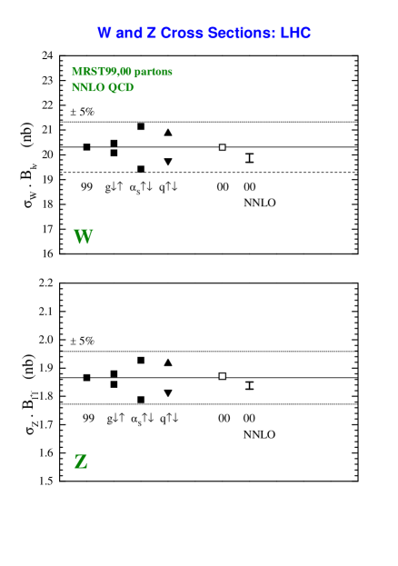
$W$ and $Z$ production in high energy $pp$ collisions have clean signatures through their leptonic decay modes, $W\rightarrow\ell\nu$ and $Z\rightarrow\ell^{+}\ell^{-}$, and so may be considered as potential luminosity monitors [44, 42, 45]. A vital ingredient is the accuracy with which the cross sections for $W$ and $Z$ production can be theoretically calculated. The cross sections depend on parton distributions, especially quark densities, in a kinematic region where they are believed to be reliably known. Recent determinations of $\sigma_{W,Z}$ at the LHC are shown in Fig. 10. The solid squares and triangles are from the NLO parton analyses of [46] and the final two predictions are from the NLO and NNLO analyses of [47]. The two major uncertainties appear to be due to the value of $\alpha_{S}$ and to using different parton densities labelled by $q\!\uparrow$ and $q\!\downarrow$. The $\alpha_{S}\!\uparrow$ and $\alpha_{S}\!\downarrow$ values correspond to changing $\alpha_{S}(M_{Z}^{2})$ by $\pm 0.005$, which is probably too conservative, so a $\pm 2\%$ uncertainty in $\sigma_{W,Z}$ is more realistic from this source. The normalisation of the input data used in the global parton analyses is another source of uncertainty in $\sigma_{W,Z}$. The HERA experiments provide almost all of the data used in the global analyses in the relevant small $x$ domain. The $q\!\uparrow$ and $q\!\downarrow$ parton sets correspond to separate global fits in which the HERA data have been renormalized by $\pm 2.5\%$ respectively. Allowing for these uncertainties, we conclude that the cross sections of $W$ and $Z$ production are known to be about $\pm 4\%$ at the LHC energy. For a precise measurement allowance should be made for $W^{+}W^{-}$ pair production and for $W$ bosons produced via $t$-quark decays, which produce about $1\%$ of the total signal.

Caron [42] discussed the experimental requirements of using $W$ and $Z$ production to determine the luminosity at the LHC.

Figure 10: The predictions of the cross sections for $W$ and $Z$ production, and leptonic decay, at the LHC [46, 47].

9 Summary on luminosity determination

The luminosity determinations based on the measurement of the forward elastic cross section and on two-photon $e^{+}e^{-}$ production can only be made in low luminosity runs, and require dedicated forward detectors and triggers. On the other hand, the measurement of $W$ or $Z$ and two-photon $\mu^{+}\mu^{-}$ production may be performed at high luminosity with the central detector. The latter process requires a good di-muon trigger with thresholds of $E_{t}\lower 3.01385pt\hbox{$\;\stackrel{{\scriptstyle\textstyle<}}{{\sim}}\;$}5$ GeV for each muon.

In principle, we may monitor the luminosity using any process, with a significant cross section, which is straightforward to detect cleanly. For example, it could be single-pion production in a given rapidity and $p_{t}$ domain or inclusive $\mu^{+}\mu^{-}$ production in a well defined kinematic region. In this way we may determine the relative luminosity and calibrate the “monitor” by comparing the number of events detected for the “monitor” reaction with the number of events for a process whose cross section is known. This has the advantage that the calibration may be carried out in a low luminosity run.

The desired goal of measuring the luminosity to better than $\pm 5\%$ definitely seems attainable. We note that for applications where it is sufficient to know the parton-parton luminosity, better accuracy can be achieved.

10 Final Observations

One view of forward or soft physics, which dominates the interactions at the LHC, is that it is an unfortunate unavoidable complication to the exciting rare events which we hope to see. It may be useful as a luminosity monitor, but the Pomeron is boring.

Another view expressed at the meeting is that to avoid the Pomeron is to deny our birthright. Almost all QCD is contained in the Pomeron. The Pomeron indirectly spawned string theory and sent a galaxy of physicists spinning off into higher dimensions. Most of the rich HERA physics is driven by the Pomeron. The ‘soft’ Pomeron in the non-perturbative domain has fascinating Regge properties, leading to glueballs and mixing with $q\bar{q}$ states. With the advent of QCD we were reminded that the quark and gluon are not elementary, but Reggeons — and that the ‘hard’ or QCD Pomeron is the compound state of two (or more) Reggeized gluons. The correct interpolation between the hard and the soft regimes is an exciting fundamental problem yet to be solved.

This meeting has offered the opportunity of a wider perspective of these two viewpoints. Moreover, we were able to glimpse the great potential, and the experimental challenges, of the LHC.

It is a special pleasure to thank, on behalf of all of the participants, Dan-Olof Riska, Risto Orava and the other members of the organizing committee, together with Laura Salmi, for arranging such an excellent Workshop, and for their hospitality in Helsinki. I gratefully acknowledge the help that I have received from Aliosha Kaidalov, Valery Khoze, Misha Ryskin and Stefan Tapprogge on the subject of this Workshop.

References

- [1] J.D. Bjorken, Int. J. Mod. Phys. A7 (1992) 4189.
- [2] F. Gianotti and M. Pepe-Altarelli, Nucl. Phys. Proc. Suppl. 89 (2000) 177.
- [3] S. Tapprogge, these proceedings.
- [4] M. Bozzo, these proceedings.
- [5] V. Nomokonov, these proceedings.
- [6] K. Piotrzkowski, these proceedings; Phys. Rev. D63 (2001) 071502(R).
- [7] W. Guryn, these proceedings.
- [8] M.M. Block, these proceedings (talk 2).
- [9] A.A. Vorobyov, these proceedings.
- [10] V.A. Khoze, A.D. Martin and M.G. Ryskin, Eur. Phys. J. C18 (2000) 167.
- [11] L.N. Lipatov, these proceedings.
- [12] A. Martin, these proceedings.
- [13] S. Mandelstam, Nuovo Cimento 30 (1963) 1113, 1127.
- [14] V.A. Abramovskii, V.N. Gribov and O. Kancheli, Sov. J. Nucl. Phys. 18 (1974) 308.
- [15] P.V. Landshoff, these proceedings.
- [16] A.B. Kaidalov, these proceedings.
- [17] K.A. Ter-Martirosyan, ITEP reports 70,71 (1975); 7,11,133–135,158 (1976).
- [18] A.B. Kaidalov, Phys. Rep. 50 (1979) 157.
- [19] P. Schlein, these proceedings.
-
[20]
M.M. Block, these proceedings (talk 1) and references therein;
M.M. Block and F. Halzen, hep-ph/0101022. - [21] E. Gotsman, E. Levin and U. Maor, Phys. Lett. B452 (1999) 387.
- [22] A.B. Kaidalov, L.A. Ponomarev and K.A. Ter-Martirosyan, Sov. J. Nucl. Phys. 44 (1986) 468.
- [23] V.A. Khoze, A.D. Martin and M.G. Ryskin, Nucl. Phys. Proc. Suppl. 99 (2001) 213.
- [24] Yu.L. Dokshitzer, V.A. Khoze and S.I. Troyan, Sov. J. Nucl. Phys. 46 (1987) 712.
- [25] J.D. Bjorken, Phys. Rev. D47 (1993) 101.
- [26] E. Gotsman, E. Levin and U. Maor, Phys. Rev. D60 (1999) 094011 and references therein.
- [27] V.A. Khoze et al., these proceedings and references therein.
- [28] M.G. Albrow and A. Rostovtsev, hep-ph/0009336.
- [29] M.L. Good and W.D. Walker, Phys. Rev. 126 (1960) 1857.
- [30] V.N. Gribov, Sov. Phys. JETP 19 (1969) 483.
- [31] J. Pumplin, Physica Scripta 25 (1982) 191.
- [32] G. Snow, these proceedings.
- [33] CDF Collaboration: T. Affolder et al., Phys. Rev. Lett. 84 (2000) 5043.
- [34] P. Marage, these proceedings.
- [35] A.B. Kaidalov et al., in preparation.
[36]
G.P. Salam, JHEP 9807 (1998) 19;
M. Ciafaloni, D. Colferai and G.P. Salam, Phys. Rev. D60 (1999) 114036;
R.S. Thorne, Phys. Lett. B474 (2000) 372; hep-ph/0103210;
see also J. Kwiecinski, A.D. Martin and P.J. Sutton, Zeit. Phys. C71 (1996) 585. - [37] W.J. Stirling, these proceedings.
- [38] J. Andersen et al., JHEP 0102:007 (2001).
- [39] A. De Roeck, these proceedings.
- [40] M.A. Kimber, J. Kwiecinski and A.D. Martin, hep-ph/0101099, Phys. Lett. B (in press).
- [41] A.G. Shamov and V.I. Telnov, these proceedings.
- [42] B. Caron, these proceedings.
- [43] See, for example, V.M. Budnev, I.F. Ginzburg, G.V. Meledin and V.G. Serbo, Phys. Lett. B39 (1972) 526.
[44]
H.J. Frisch, CDF/PHYSICS/PUBLIC/2484 (1994);
M. Dittmar, F. Pauss and D. Zürcher, Phys. Rev. D56 (1997) 7284. - [45] V.A. Khoze, A.D. Martin, R. Orava and M.G. Ryskin, hep-ph/0010163, Eur. Phys. J. C (in press).
- [46] A.D. Martin, R.G. Roberts, W.J. Stirling and R.S. Thorne, Eur. Phys. J. C14 (2000) 133.
- [47] A.D. Martin, R.G. Roberts, W.J. Stirling and R.S. Thorne, Eur. Phys. J. C18 (2000) 117.
- [48] FELIX proposal, CERN/LHCC 97-45, LHCC/I10 (1997).