Very light CP-odd scalar in the Two-Higgs-Doublet Model

Abstract

We show that a general two-Higgs-doublet model (THDM) with a very light CP-odd scalar ($A$) can be compatible with $\rho$ parameter, Br($b\to s\gamma$), $R_{b}$, $A_{b}$, $(g-2)_{\mu}$ of muon, Br($\Upsilon\to A\gamma$), and the direct search via the Yukawa process at LEP. For its mass around 0.2 GeV, the muon $(g-2)_{\mu}$ and Br($\Upsilon\to A\gamma$) data require $\tan\beta$ to be about 1. Consequently, $A$ can behave like a fermiophobic CP-odd scalar and predominantly decay into a $\gamma\gamma$ pair, which registers in detectors of high energy collider experiments as a single photon signature when the momentum of $A$ is large. We compute the partial decay width of $Z\to AAA$ and the production rate of $f\bar{f}\to ZAA\to Z+\/"\gamma\gamma"$, $f^{\prime}{\bar{f}}\to W^{\pm}AA\to W^{\pm}+\/"\gamma\gamma"$ and $f\bar{f}\to H^{+}H^{-}\to W^{+}W^{-}AA\to W^{+}W^{-}+\/"\gamma\gamma"$ at high energy colliders such as LEP, Tevatron, LHC, and future Linear Colliders. Other production mechanisms of a light $A$, such as $gg\to h\to AA\to"\gamma\gamma"$, are also discussed.

I Introduction

One of the main tasks of the current and future high energy colliders is to find the Higgs boson of the Standard Model (SM), or some other scalar particle(s), if there is any, predicted by the extensions of the SM. The mass spectrum of these scalars as well as their decay channels depend on the assumed model. Recently, the possibility of a Higgs boson decaying into a pair of light CP-odd scalars was considered in Ref. [1]. As pointed out in that paper, a very light CP-odd scalar ($A$) can arise in some extensions of the SM, such as the minimal composite Higgs model [2], or the next-to-minimal supersymmetric model [3]. An interesting aspect of a light $A$ particle is that if its mass ($M_{A}$) is less than twice of the muon mass ($m_{\mu}$), i.e. less than about 0.2 GeV, it can only decay into a pair of electrons ($A\to e^{+}e^{-}$) or photons ($A\to\gamma\gamma$). Hence, the decay branching ratio Br($A\to\gamma\gamma$) can be sizable. Furthermore, at high energy colliders, the light CP-odd scalar $A$ can be produced with such a large velocity that the two photons from its decay are highly boosted and seen by the detector as one single-photon signature. Therefore, the production of a pair of $AA$ is identified by the detector as a pair of photons when each $A$ decays into its diphoton mode. The subsequent signature as a diphoton resonance (e.g., in the case that a Higgs boson decays into a pair of $A$) or photon cascades (e.g., in the case that a $A$ particle is radiated from a fermion line) provides an interesting window for the experimental search of the scalar particles that may be responsible for the breaking of the electroweak symmetry . In general, we expect the decay branching ratio of $A\to\gamma\gamma$ to decrease rapidly when the di-muon channel ($A\to\mu^{+}\mu^{-}$) becomes available as $M_{A}$ increases. This is because the Yukawa coupling of $A$-$\mu^{+}$-$\mu^{-}$ is larger than that of $A$-$e^{+}$-$e^{-}$ by the mass ratio $(m_{\mu}/m_{e})\sim 200$. Since we are interested in the phenomenology of having a light $A$ decaying into a pair of photons, we will restrict our discussion for $M_{A}$ less than about $0.2$ GeV, though in principle, that is not necessary as long as the decay branching ratio Br($A\to\gamma\gamma$) is not too small to be observed experimentally.

A simple extension of the SM is the two-Higgs-doublet model (THDM) [3], which has been extensively studied theoretically and experimentally. For example, a constraint on the mass of the charged Higgs boson $H^{+}$ in the THDM was carefully examined at the CERN LEP as a function of its decay branching ratios into the $\tau^{+}\nu_{\tau}$ and $c{\bar{s}}$ modes [4]. Studies on searching for a light $A$ in its associated production with a bottom quark pair were also done [5], as a function of $M_{A}$ and $\tan\beta$ (the ratio of the two vacuum expectation values of the Higgs doublets in the THDM). Though some useful constraints have been obtained by the LEP experiments, we show in this work that a very light $A$ (with $M_{A}<2m_{\mu}$) is still allowed in the THDM. This low $M_{A}$ value, in the context of a THDM, can induce large contributions to the $\rho$-parameter unless other parameters of the model adjust to counteract this effect. In particular, as to be discussed later, the masses of the charged scalar ($H^{+}$) and the heavy CP-even Higgs boson ($H$) have to be approximately equal. Also, the value of the mixing angle $\alpha$ has to be such that $\cos(\beta-\alpha)$ becomes small in order to suppress the Higgs boson contribution to the $\rho$-parameter.

Another important experimental data to constrain a light $A$ in the THDM is the measurement of the muon anomalous magnetic moment. The recent measurement at BNL [6] strongly disfavors such a model when compared with certain theory calculation [7, 8]. Nevertheless, other theory calculations of the SM contributions to the muon magnetic moment show a better agreement with the BNL data [9]. Consequently, a light $A$ in the THDM can still be compatible with data though the parameter space of such a THDM is tightly constrained.

In the next section we will examine all the relevant low energy data (including the $(g-2)_{\mu}$ of muon, Br($\Upsilon\to A\gamma$), $\rho$-parameter, $b\to s\gamma$, $R_{b}$ and $A_{b}$) to determine the allowed parameter space of the THDM with a very light $A$. In section III, we consider the decay widths and the decay branching ratios of every Higgs boson predicted in this model. In section IV, we study the potential of the light $A$ boson as a source of the distinctive photon signal at colliders. It can happen in either the decay mode of the neutral gauge boson $Z\to AAA\to\/"\gamma\gamma\gamma"$, or the production processes of Higgs bosons, such as $f\bar{f}\to ZAA\to Z+\/"\gamma\gamma"$, $f^{\prime}{\bar{f}}\to W^{\pm}AA\to W^{\pm}+\/"\gamma\gamma"$ and $f\bar{f}\to H^{+}H^{-}\to W^{+}W^{-}AA\to W^{+}W^{-}+\/"\gamma\gamma"$. Section V contains our conclusion.

II Constraints from low energy data

In the THDM, the couplings of fermions to Higgs bosons are proportional to the fermion masses. In the type-I of the THDM, only one of the two Higgs doublets couple to fermions via Yukawa couplings, and in the type-II of the THDM, one of the Higgs doublets couples to the up-type fermions (with weak isospin equal to $1/2$) and another couples to the down-type fermions (with weak isospin equal to $-1/2$). Hence, the couplings of Higgs bosons to fermions generally depend on the value of $\tan\beta$. In case that the coupling of the Higgs bosons to fermions is large and the mass of the Higgs boson is small, the radiative correction to the low energy data can be sensitive to the Yukawa interactions. Hence, the low energy data can be used to impose important constraints on the masses and the couplings of the Higgs bosons. To examine the allowed range of $M_{A}$ and $\tan\beta$ in the THDM, we shall consider the precision data on the anomalous magnetic moment of the muon, the decay branching ratio of $\Upsilon\to A\gamma$, $b\to s\gamma$, the $\rho$-parameter, the decay branching ratio of $Z\to b{\bar{b}}$, i.e. $R_{b}$, and the bottom quark asymmetry $A_{b}$ measured at the $Z$-pole.

A Constraint on $\tan\beta$ from the $(g-2)_{\mu}$ of muon

The magnetic moment of muon is defined as

$$\mu_{\mu} = (1+a_{\mu})\frac{e\hbar}{2m_{\mu}},$$ (1)

$${\rm with}\qquad\qquad a_{\mu} \equiv \frac{(g-2)_{\mu}}{2}\;,$$ (2)

where $a_{\mu}$ is the muon anomalous magnetic moment, which is induced from radiative corrections. The SM prediction includes the QED, weak and hadronic contributions. Among them, the hadronic contribution has the largest uncertainty, and the bulk of the theoretical error is dominated by the hadronic vacuum polarization (h.v.p.). There are a number of evaluations of the h.v.p. corrections; four recent results were extensively discussed in Ref. [9]. After comparing various theory model predictions with the precise experimental data, which is

$$10^{11}\times a_{\mu}(\hbox{experiment})=116\,592\,023\pm 140\pm 60\,,$$

Ynduráin concluded that the discrepancies between the world averaged experiment data (exp.) and the theory prediction of the SM contribution (theo.) are [9]:

$$10^{11}\times\Delta a_{\mu}(\hbox{exp. -- theo.})= 422\pm 152(\hbox{exp.})\pm 77(\hbox{theo.})\quad\hbox{(DH)}$$ (3)

$$10^{11}\times\Delta a_{\mu}(\hbox{exp. -- theo.})= 358\pm 152(\hbox{exp.})\pm 112(\hbox{theo.})\quad\hbox{(J)}$$ (4)

$$10^{11}\times\Delta a_{\mu}(\hbox{exp -- theo.})= 233\pm 152(\hbox{exp.})\pm 104(\hbox{theo.})\quad\hbox{(AY)}$$ (5)

$$10^{11}\times\Delta a_{\mu}(\hbox{exp. -- theo.})= 119\pm 152(\hbox{exp.})\pm 115(\hbox{theo.})\quad\hbox{(CLY)}$$ (6)

In the above result, DH stands for the analysis of Ref. [10], J for that, as yet unpublished, of F. Jegerlehner, quoted in Ref. [7], AY indicates the result of Ref. [11], and CLY is the ‘old’ result of Ref. [12] after being corrected for the new favored value of higher order hadronic corrections [9].

In the general THDM, as well as in supersymmetric models, $a_{\mu}$ can receive radiative corrections at the one loop level from the couplings of $A$, $h$ and $H$ to muons in triangle diagrams (see Appendix A) [3, 13, 14]. As expected, the size of the radiative corrections is proportional to the coupling of muon to Higgs bosons. Moreover, the loop integral reaches its maximal value when the mass of the scalar boson in the loop becomes negligible, and diminishes as the scalar mass increases. It was concluded in Ref. [8] that a light CP-even Higgs boson ($h$) can be responsible for the apparent deviation of the BNL measurement of $a_{\mu}$ from the DH prediction of the SM contribution, at the 90% confidence level ( CL), in the framework of a type-II THDM, in which the other Higgs bosons are heavy (of the order of 100 GeV). It was found that the model parameters have to satisfy the following requirements:

$$m_{\Upsilon}\mathrel{\raise 1.29167pt\hbox{$<$\kern-7.5pt\lower 4.30554pt\hbox{$\sim$}}}M_{h}\mathrel{\raise 1.29167pt\hbox{$<$\kern-7.5pt\lower 4.30554pt\hbox{$\sim$}}}2m_{B}\;,$$ (7)

$$\sin(\beta-\alpha)\simeq 0\;,$$ (8)

$$30\mathrel{\raise 1.29167pt\hbox{$<$\kern-7.5pt\lower 4.30554pt\hbox{$\sim$}}}\tan\beta\mathrel{\raise 1.29167pt\hbox{$<$\kern-7.5pt\lower 4.30554pt\hbox{$\sim$}}}35\;.$$ (9)

In the case that only $A$ is light and the other Higgs bosons are heavy, the one-loop contribution to $a_{\mu}$ is negative. Therefore, this type of new physics is strongly disfavored according to the theory prediction of the SM contribution provided by DH; however, it can still be compatible with the other SM theory calculations (cf. Eq. 6). Furthermore, it was found in Ref. [15] that a two-loop contribution to $a_{\mu}$ can be sizable when $A$ is light. As compared to the one-loop graph, a two-loop graph can contain a heavy fermion loop. The Yukawa coupling of the heavy fermion (with mass $m_{f}$) in the second loop together with the mass insertion of the heavy fermion will give rise to $(m_{f}/m_{\mu})^{2}$ enhancement which can overcome the extra loop suppression factor of $1/16\pi^{2}$. Because the two-loop contribution can be even larger than the one-loop contribution, the contribution from a light $A$ to $a_{\mu}$ can become positive when $M_{A}$ is not too small. Hence, in general, a two-loop calculation of a light $A$ contribution to the muon magnetic moment $a_{\mu}$ yields a better agreement with the experimental data than a one-loop calculation. For that reason, in the following numerical analysis, we shall apply the two-loop calculation presented in Ref. [15] to test the compatibility of a light A THDM to the experimental data (cf. Eq. 6). For completeness, we summarize the relevant formula in Appendix A to clarify the contributions included in our numerical analysis.

Although we are using a two-loop calculation for our numerical analysis, it is useful to examine a few features predicted by the one-loop calculation. Since a one-loop contribution to $a_{\mu}$ from a light $A$ is always negative and the central value of $a_{\mu}(\hbox{exp. -- theo.})$ is positive, the potentially large loop contribution to $a_{\mu}$ has to be suppressed by a small Yukawa coupling in order for the model to be compatible with data. For a type-II THDM, this implies a very stringent bound on $\tan\beta$, because the coupling of muon to $A$ is directly proportional to $\tan\beta$. (The coupling strength of $A$-$\mu^{+}$-$\mu^{-}$ in the type-II model is $(m_{\mu}/v)\tan\beta$, where $v$ is the weak scale, $\sim 246$ GeV.) In particular, assuming the CLY prediction for the SM contribution and applying the two-loop calculation to include the light $A$ contribution, we find that there exists an upper bound on $\tan\beta$ at the 95% CL. For a 0.2 GeV pseudo-scalar,

$$\tan\beta<2.6\;.$$ (10)

This new bound is stronger by a factor of two than a previous one [16], which was obtained from the one loop contribution, together with the old experimental data with an error of $84\times 10^{-10}$ in the measurement of $(g-2)_{\mu}$. In Fig. 1, we show the regions in the $\tan\beta$ versus $M_{A}$ plane allowed by the $a_{\mu}$ data at the 95% CL. Three different curves are displayed depending whether the SM prediction is given by the CLY, AY or J calculation. There is no allowed region according to the DH calculation. For the type-II THDM, the allowed regions are below the curves, for the type-I THDM, they are above the curves. For completeness, we also show in Figs. 2 and 3 the allowed regions in the type-I and type-II THDM, respectively, for a wide range of $M_{A}$ and $\tan\beta$. In the above figures we did not show the constraints derived from the CUSB Collaboration search for $\Upsilon\to A\gamma$ at CESR [17]. For that, we refer the readers to Ref. [3] which has an extensive discussion on this data to constrain a light CP-even or CP-odd scalar in the THDM. As noted there, various theory analyses indicated that the high order QCD corrections to this decay rate can be large. Because of that, we shall consider in this paper $\tan\beta$ around 1 to be consistent with the CUSB data for a 0.2 GeV pseudoscalar. Specifically, we shall take $\tan\beta$ to be either 0.5 or 2 in our following discussions.

Finally, we note that a similar constraint on $\tan\beta$ can be obtained from examining the production of $e^{-}e^{+}\to b{\bar{b}}A$ at LEP energies [5]. However, as shown in Ref. [16], the $(g-2)_{\mu}$ data gives a more stringent constraint than that obtained from direct searches of Higgs bosons via the above Yukawa process.

B Constraint on $M_{H^{+}}$ from the decay of $b\to s\gamma$

The previous $(g-2)_{\mu}$ analysis is only sensitive to a light pseudoscalar $A$ when the masses of the CP-even scalars $h$, $H$ and the charged Higgs boson $H^{\pm}$ are all of the order of hundred GeV. To further constrain the parameter space of the THDM, we now turn our attention to a low energy observable that is sensitive to a charged Higgs boson in case that $\tan\beta$ is not large. That is the rare decay process $b\to s\gamma$.

For the hadronic flavor changing neutral current decay process $b\to s\gamma$, new physics effects at the weak scale can be parameterized by the couplings (Wilson coefficients) of an effective Hamiltonian [18]. The only scalar contribution to the Wilson coefficient $C_{7}$ in a THDM comes from the standard penguin diagram, where the charged Higgs scalar $H^{\pm}$ couples to top and bottom, and then to top and strange quarks.

The $H^{\pm}tb$ coupling in the type-II THDM is given by

$${\cal L}=\sqrt{2}V_{tb}\left\{\frac{m_{b}}{v}\tan\beta\;{\overline{t}_{L}}b_{R}+\frac{m_{t}}{v}\cot\beta\;{\overline{t}_{R}b_{L}}\right\}H^{+}+\rm{h.c.}\;$$ (11)

where $V_{tb}$ is the Cabbibo-Kobayashi-Maskawa (CKM) matrix element. The $H^{\pm}ts$ coupling is defined similarly with the appropriate substitution $b\to s$. In the type-I model, the factor $\tan\beta$ is substituted by $-\cot\beta$. For a type-II model, a value of $\tan\beta<1$ will induce a large ${\overline{t}_{R}}b_{L}H^{+}$ coupling, which will strongly modify the Wilson coefficient $C_{7}$ and then increase the predicted $b\to s\gamma$ rate. This can be alleviated only if the charged $H^{+}$ is massive enough.

Constraints on $\tan\beta$ versus $M_{H^{+}}$ have been obtained by F. Borzumati and C. Greub in the first reference of [19] for a few possible experimental upper bounds on Br$(\bar{B}\to X_{s}\gamma)$, ranging from $3.0\times 10^{-4}$ to $4.5\times 10^{-4}$. Currently, the reported experimental measurements are

$${\rm Br}(\bar{B}\to X_{s}\gamma)\times 10^{4} = 3.15\pm 0.35_{stat}\pm 0.32_{sys}\pm 0.26_{model}\;\;{\rm by\,CLEO\cite[cite]{[\@@bibref{Number}{cleo}{}{}]},}$$ (12)

$${\rm Br}(\bar{B}\to X_{s}\gamma)\times 10^{4} = 3.11\pm 0.80_{stat}\pm 0.72_{sys}\;\;{\rm by\,ALEPH\cite[cite]{[\@@bibref{Number}{bsgaleph}{}{}]},}$$ (13)

$${\rm Br}(\bar{B}\to X_{s}\gamma)\times 10^{4} = 3.36\pm 0.53_{stat}\pm 0.42_{sys}(^{0.50}_{0.54})_{model}\;\;{\rm by\,BELLE\cite[cite]{[\@@bibref{Number}{belle}{}{}]}}.$$ (14)

In this study, we will quote the result given in Ref. [19] for an upper bound of 4.5$\times 10^{-4}$ on Br$(\bar{B}\to X_{s}\gamma)$. It was found that, for example, if $\tan\beta=0.4$, the mass of $H^{+}$ must be larger than about 300 GeV. On the other hand, we will not use the detailed information on the lower bounds of $M_{H^{+}}$ for $\tan\beta<1$, because in that case we would rather use the stronger bounds obtained from examining the $b{\bar{b}}$ decay rate of the $Z$-boson, i.e. $R_{b}$ (see next section). When $\tan\beta$ is much greater than 1, the small effect from the ${\overline{t}_{R}}b_{L}H^{+}$ coupling is compensated by the large effect from the ${\overline{t}_{L}}b_{R}H^{+}$ coupling; in such a way that the Br$(b\to s\gamma)$ prediction tends to stay at a certain minimal value. This minimum only requires $M_{H^{+}}>165$ GeV for $\tan\beta\gg 1$. In summary, for $\tan\beta>1$, the Br$(b\to s\gamma)$ data requires $M_{H^{+}}>165$ to 200 GeV at the 95% CL.

The situation for type-I models is different. In this case, both the ${\overline{t}_{R}}b_{L}H^{+}$ and ${\overline{t}_{L}}b_{R}H^{+}$ couplings decrease for values of $\tan\beta$ greater than 1. This does not mean that $M_{H^{+}}$ can become arbitrarily small. There is an unstable behavior (due to the large scale dependence) for the prediction of Br$(b\to s\gamma)$ when $M_{H^{+}}$ is less than about 100 GeV and $\tan\beta\sim 1$ [19]. This problem of unstability gets worse when $\tan\beta<1$.

C Constraint on $M_{H}-M_{H^{+}}$ from $\Delta\rho$

The effect of scalar fields ($A$, $h$, $H$ and $H^{+}$) on $\Delta\rho$ have been reported for a general THDM in the literature [23, 24, 25]. When $M_{A}$ becomes negligible, the contribution to $\Delta\rho$ can grow quadratically with the masses of the other scalars (See the appendix of Ref. [25]). The only way to keep $\Delta\rho$ small is to have cancellations among potentially large loop contributions from each Higgs boson. For example, as $\sin^{2}(\beta-\alpha)=1$, this cancellation can take place between the contributions from $H^{\pm}$ and $H$, and requires a certain correlation between their masses. ($\alpha$ is the mixing parameter between the two CP-even Higgs bosons $h$ and $H$.) As shown in the appendix of Ref. [25], this correlation depends on the value of the coefficient $\sin^{2}(\beta-\alpha)$. In Fig. 4 we show the different allowed regions in the $M_{H^{+}}$ versus $M_{H}$ plane for three different values of $\sin^{2}(\beta-\alpha)$. These regions or bands correspond to the 95 % CL limits for $\Delta\rho$ [25] with

$$-1.7\;<\;\Delta\rho\times 10^{3}\;<\;2.7.$$ (15)

For simplicity, we shall assume $M_{H}\sim M_{H^{+}}$ and $\sin^{2}(\beta-\alpha)=1$ for our detailed numerical analysis. It should be noted that the allowed band for $\sin^{2}(\beta-\alpha)=1$ only depends on $M_{H}$ and $M_{H^{+}}$, whereas the allowed bands for $\sin^{2}(\beta-\alpha)<1$ do depend on $M_{h}$. In Fig. 4 we have used a low value of $M_{h}=110$ GeV. If we use a higher value, for instance $M_{h}=130$ GeV, the bands keep the same width but slightly shift downwards (to a somewhat smaller slope).

We have checked that within the allowed parameter space constrained by the $\rho$-parameter, the new physics contribution from the THDM with a light $A$ to the S-parameter is typically small as compared to the current data: $\Delta S=-0.07\pm 0.11$ [26]. Using the analytical result in Ref. [27], we find that $\Delta S$ approximately equals to $-0.02$ when $M_{H}$ and $M_{H^{+}}$ are about the same, and reach $-0.05$ when $M_{H}$ and $M_{H^{+}}$ differ by a few hundred GeV. Although $\Delta S$ can reach $-0.1$ when $M_{H}$ and $M_{H^{+}}$ differ by about a TeV, this choice of parameters is already excluded by the $\rho$-parameter measurement. Hence, we conclude that the current $S$-parameter measurement does not further constrain this model. Needless to say that the above conclusion holds for both the type-I and type-II THDM at the one-loop order.

D Constraint on $M_{H^{+}}$ versus $\tan\beta$ from $R_{b}$ and $A_{b}$

The contributions to the $Z\to b\overline{b}$ hadronic decay branching ratio ($R_{b}$) and the forward-backward asymmetry ($A_{b}$) of the bottom quark in $Z$ decays are given in terms of the effective $Zb\overline{b}$ couplings [25]:

$${\cal L} = \frac{e}{s_{w}c_{w}}\Big{(}g_{L}\;{\overline{b}_{L}}\gamma^{\mu}b_{L}\;+\;g_{R}\;{\overline{b}_{R}\gamma^{\mu}b_{R}}\Big{)}\;Z_{\mu}\;,$$ (16)

$$g_{L} = -{\frac{1}{2}}+\frac{1}{3}s^{2}_{w}\,+\,\delta g_{L}\;,$$ (17)

$$g_{R} = \frac{1}{3}s^{2}_{w}\,+\,\delta g_{R}\;.$$ (18)

Here, $\delta g$’s contain the SM as well as the new physics (THDM) contributions at one loop order:

$$\delta g_{L} = \delta g_{L}^{SM}+\delta g_{L}^{new}\;=\;-0.4208+\delta g_{L}^{new},$$ (19)

$$\delta g_{R} = \delta g_{R}^{SM}+\delta g_{R}^{new}\;=\;0.0774+\delta g_{R}^{new}\;,$$ (20)

where the SM values are for $m_{t}=174$ GeV and $M_{h}=100$ GeV [28]. Because of the left-handed nature of the weak interaction, the value of $g_{L}$ is higher (by about 5 times) than $g_{R}$.

As shown previously, the $(g-2)_{\mu}$ data requires $\tan\beta$ to be less than about 2.6 for a 0.2 GeV $M_{A}$. In that case, the contribution from the neutral Higgs boson loops to $R_{b}$ is negligible and the dominant contribution comes from the charged Higgs boson loop [25]. For a small $\tan\beta$, the $H^{+}$ loop contribution comes mostly from the ${\overline{t}_{R}b_{L}}H^{+}$ coupling, which is proportional to $(m_{t}/v)\,\cot\beta$, cf. Eq. (21). Since the type-I and type-II models coincide on this coupling, the bounds from the $R_{b}$ measurement applies to both of the models. The $H^{+}$ loop contributions to $\delta g_{L}$ and $\delta g_{R}$ are given by

$$\delta g_{L}^{new} = \frac{1}{16\pi^{2}}\left(\frac{m_{t}}{v}\cot\beta\right)^{2}\left(\frac{R}{R-1}-\frac{R\log R}{(R-1)^{2}}\right)\;,$$ (21)

$$\delta g_{R}^{new} = -\frac{1}{16\pi^{2}}\left(\frac{m_{b}}{v}\tan\beta\right)^{2}\left(\frac{R}{R-1}-\frac{R\log R}{(R-1)^{2}}\right)\;,$$ (22)

with $R\equiv m_{t}^{2}/M^{2}_{H^{+}}$. Expanding $R_{b}$ and $A_{b}$ to first order in $\delta g_{R}^{new}$ and $\delta g_{L}^{new}$, we obtain

$$R_{b} = R_{b}^{SM}-0.7785\delta g_{L}^{new}+0.1409\delta g_{R}^{new},$$ (23)

$$A_{b} = A_{b}^{SM}-0.2984\delta g_{L}^{new}-1.6234\delta g_{R}^{new}\;,$$ (24)

with $R_{b}^{SM}=0.2158$ and $A_{b}^{SM}=0.935$. As indicated in the above equation, $A_{b}$ depends more on $g_{R}$ than on $g_{L}$; the opposite is true for $R_{b}$. For this reason, and because the experimental uncertainty of $R_{b}$ is significantly smaller than that of $A_{b}$, the asymmetry $A_{b}$ is not nearly as effective to constrain the parameter region of the THDM than $R_{b}$ when $\tan\beta$ is of the order of 1. Hence, in this work, we will only consider the constraints imposed by the $R_{b}$ measurement, for which the experimental limits are [29]:

$$R^{Exp}_{b} = 0.21648\;\pm\;0.00075\;.$$ (25)

The allowed region, at the 95% CL, in the $\tan\beta$ versus $M_{H^{+}}$ plane is shown in Fig. 5, in which the constraints imposed by the $(g-2)_{\mu}$ and the $b\to s\gamma$ data are also included. It is interesting to compare our $R_{b}$ bound (the lower solid curve) with the Fig. 6.1 of Ref. [25] (same as the Fig. 5 of Ref. [24]). There, the experimental central value used for $R_{b}$ was 0.21680, with a smaller ($1\sigma$) error of $\pm 0.00073$. Since the new $R^{Exp}_{b}$ is only $0.81\sigma$ above the SM value that we use here, the bounds on $M_{H^{+}}$ become less stringent.

In summary, Fig. 5 shows the allowed region in the $\tan\beta$ versus $M_{H^{+}}$ plane for the type-I and type-II models with a light (0.2 GeV) CP-odd scalar $A$. The $(g-2)_{\mu}$ data imposes an upper bound on $\tan\beta$ for a type-II THDM, and the value of this upper bound depends on the model of theory calculations. Note that there is no DH curve in the figure. This is because a THDM with a very light $A$ cannot be compatible with data according to the DH calculation of the SM contribution to $a_{\mu}$. Similarly, the lower bound on $\tan\beta$ imposed by the $(g-2)_{\mu}$ data for a type-I THDM can be easily obtained from Fig. 1. The lower bound from $R_{b}$ holds for either type-I or type-II THDM, and is not sensitive to the actual value of the mass of the light $A$, because for $\tan\beta\sim 1$ the charged Higgs boson loop dominates. A similar conclusion also holds for the constraint imposed by the $b\to s\gamma$ data. Furthermore, the $b\to s\gamma$ data does not provide a useful constraint for a type-I model when $\tan\beta>1$. For clarity, we summarize the constraints from the relevant low energy data in Table I for each type of THDM. Although in the type-II THDM, the value of $\tan\beta$ is bounded from above to be less than about 2.6, it can take on any value above the lower bound imposed by the $R_{b}$ data. On the other hand, the value of $\tan\beta$ in the type-I model cannot be too large because for a very large value of $\tan\beta$, the decay width of the lighter CP-even Higgs boson ($h$) can become as large as its mass, so that the model ceases to be a valid effective theory.

In the next section, we shall discuss the decay and production of the Higgs bosons in the THDM with a light $A$. For simplicity, we shall only discuss the event rates predicted by a type-II model, and the value of $\tan\beta$ is taken to be either 0.5 or 2 to be consistent with all the low energy data discussed in this section. As shown in Fig. 5, in a type-II THDM with a light $A$, the masses of the Higgs bosons other than the light CP-even Higgs boson $h$ have to be around 1 TeV when $\tan\beta=0.5$. Hence, its phenomenology can be very different from the model with $\tan\beta=2$, in which a few hundred GeV heavy Higgs boson $H$ and charged Higgs boson $H^{\pm}$ are allowed.

III Decay Branching Ratios of Higgs Bosons

In this section, we shall examine the decay branching ratios of the Higgs bosons predicted by the type-II THDMs with a very light CP-odd scalar $A$. To be consistent with the $\rho$-parameter analysis, the mixing angle $\alpha$ as well as the Higgs boson masses $M_{H^{+}}$ and $M_{H}$ have to be correlatively constrained, cf. Fig. 4. Without losing generality, in this section we shall assume $\sin(\beta-\alpha)=1$ to simplify our discussion.

As noted in the previous sections, a CP-odd scalar $A$, with its mass around 0.2 GeV, can only decay into a $e^{-}e^{+}$ pair or a photon pair. Though the decay process $A\to\gamma\gamma$ can only occur at loop level, its partial decay width may compete with the tree level process $A\to e^{-}e^{+}$. This is because the mass of the electron is very tiny as compared to the electroweak scale $v$, and the partial decay width of $A\to e^{-}e^{+}$ is suppressed by ($m_{e}/v)^{2}$.

To clarify our point, we note that for $\alpha=\beta-\pi/2$, the couplings of Higgs bosons and fermions in the THDM are given by

$${\cal L}_{\overline{f}fS} =- \frac{m_{f}}{v}{\overline{f}}fh\;-\;X\frac{m_{d}}{v}\overline{d}dH\;+\;Y\frac{m_{u}}{v}\overline{u}uH$$ (26)

$$+ iX\frac{m_{d}}{v}\overline{d}\gamma^{5}dA\;+\;iY\frac{m_{u}}{v}\overline{u}\gamma^{5}uA,$$ (27)

where $X=\tan\beta$, $Y=\cot\beta$ for the type-II model, and $X=-\cot\beta$, $Y=\cot\beta$ for the type-I model. (Here, $f$ stands for any fermion, $u$ for an up-type fermion, and $d$ for an down-type fermion.) Therefore, the partial decay widths of Higgs bosons into fermion pairs are:

$$\Gamma_{{S_{i}}\to f{\bar{f}}} = \frac{N_{c}}{8\pi}C_{{\overline{f}}fS}^{2}M_{S_{i}}\left(1-4\frac{m^{2}_{f}}{M^{2}_{S_{i}}}\right)^{3/2},\,{\rm with}\,{S_{i}}=h\,\,\/{\rm or}\/\,\,H,$$ (28)

$$\Gamma_{A\to f{\bar{f}}} = \frac{N_{c}}{8\pi}C_{{\overline{f}}fA}^{2}M_{A}\left(1-4\frac{m^{2}_{f}}{M^{2}_{A}}\right)^{1/2},$$ (29)

where $C_{{\overline{f}}f{S_{i}}}=\frac{m_{f}}{v}\times$(1, $X$, or $Y$ ) is the coupling defined in ${\cal L}_{\overline{f}fS}$, and $N_{c}$ is the color factor (which is 3 for quarks and 1 for leptons).

The partial decay width of $A\to\gamma\gamma$ at the one-loop order arises from fermion loop contributions, which yield [3]:

$$\Gamma\left(A\to\gamma\gamma\right)=\frac{\alpha^{2}g^{2}}{256\pi^{3}}\frac{M_{A}^{3}}{m_{W}^{2}}\left|H\right|^{2},$$ (30)

$$H=\sum_{f}N^{f}_{c}\,Q_{f}^{2}\,C_{f}\,\tau_{f}\,F\left(\tau_{f}\right)$$ (31)

where $\tau_{f}=(2m_{f}/M_{A})^{2}$, $N^{f}_{c}=1\,(3)$ for leptons (quarks), $Q_{f}$ and $m_{f}$ are the electric charge (in units of $e$) and the mass of fermion, respectively. Also, $C_{f}=\cot\beta\,(\tan\beta)$ for up-type quarks (charged leptons and down-type quarks) in a type-II THDM. Furthermore, $F(x)$ is given by

$$F(x)=\left\{\begin{array}[]{ll}\left(\arcsin\frac{1}{\sqrt{x}}\right)^{2}&\qquad{\rm for}\;x\geq 1\\ -\left({\mathrm{arccosh}}\frac{1}{\sqrt{x}}-\,\frac{i\,\pi}{2}\right)^{2}&\qquad{\rm for}\;x<1,\end{array}\right.$$ (32)

In Figs. 6 and 7, we show the life-time (multiplied by the speed of light) of $A$ and its partial decay branching ratio Br($A\to\gamma\gamma$), as a function of $\tan\beta$ for various $M_{A}$ values. As indicated, the typical life-time of a light CP-odd scalar $A$ (with mass around 0.2 GeV and $\tan\beta$ around 1) is about $10^{-3}$ meter, so the decay length of a 50 GeV $A$ boson is about 0.25 meter. This unique feature of a light scalar $A$ boson can be used to improve identifying such an event experimentally. For $\tan\beta\sim 1$, about half of the time, the light $A$ can decay into a photon pair, other than a $e^{-}e^{+}$ pair. Because $A$ is usually produced with a large velocity in collider experiments, the two decay photons will be largely boosted and seen by the detector (the electromagnetic calorimeter) as if it were a single-photon signal.

To discuss the decay branching ratios of the other Higgs bosons, we need to specify all the parameters in the scalar sector of the THDM Lagrangian. In a CP-conserving THDM Lagrangian with natural flavor conservation (ensured by the discrete symmetry of $\phi_{1}\to\phi_{1}$ and $\phi_{2}\to-\phi_{2}$), there are eight parameters in its Higgs sector [25]. They are $m_{1}$, $m_{2}$, $\lambda_{1,2,3,4,5}$, and $\mu_{12}$, or equivalently, $M_{h}$, $M_{H}$, $M_{H^{+}}$, $M_{A}$, $\alpha$, $\tan\beta$, $v$, and $\mu_{12}$. Of these eight free parameters, seven have been addressed in the previous section: four Higgs boson masses, two mixing angles ($\alpha$ and $\beta$) and the vacuum expectation value $v$. There is yet another free parameter: the soft breaking $\mu_{12}$ term that so far has not been constrained. This is because up to the one loop order, $\mu_{12}$ does not contribute to the low energy data discussed above. With the assumption $\alpha=\beta-\pi/2$ we can write the $hAA$, $HAA$, $HAZ$ and $H^{+}AW$ couplings as follows:

$${\cal L} = \frac{1}{2}\lambda_{h}hAA\;+\;\frac{1}{2}\lambda_{H}HAA\;+$$ (33)

$$\lambda_{HAZ}\;Z^{\mu}(H\partial_{\mu}A-A\partial_{\mu}H)\;+\;\lambda_{H^{+}AW}\;\left[W^{-}_{\mu}(H^{+}\partial^{\mu}A-A\partial^{\mu}H^{+})+\rm{h.c.}\right],$$ (34)

where the coupling constants are given by

$$\lambda_{h} = \frac{(2M^{2}-M^{2}_{h})}{v},$$ (35)

$$\lambda_{H} = 2\frac{M_{H}^{2}-M^{2}}{v\tan 2\beta},$$ (36)

$$\lambda_{HAZ} = \frac{-e}{2s_{W}c_{W}},$$ (37)

$$\lambda_{H^{+}AW} = \frac{-e}{2s_{W}},$$ (38)

with $M^{2}={\mu^{2}_{12}}/({\sin\beta\,\cos\beta})$. For a very light $A$, both the total width and the decay branching ratios of the other Higgs bosons in the model can be strongly modified to differ from the usual predictions of the THDM (with $M_{A}$ at the weak scale $v$).

At tree level, the partial decay width of $h\to AA$ (or $H\to AA$) is given by

$$\Gamma_{(H)h\to AA}=\frac{\lambda^{2}_{(H)h}}{32\pi M_{(H)h}}.$$ (39)

It turns out that $h\to AA$ is always the dominant (more than 90%) decay channel of $h$ except when $2M^{2}\simeq M^{2}_{h}$, in which case the $hAA$ coupling is diminishing. When the parameter $\mu_{12}$ increases, the decay width of the light Higgs boson can become large. For instance, for $M_{h}=110$ GeV and $\mu_{12}=200$ GeV, $\Gamma_{h\to AA}=34$ GeV and 54 GeV for $\tan\beta=1$ and 2, respectively. Hence, in order for the considered model to be a valid effective theory we shall restrict the range of the parameter $\mu_{12}$ so that the decay width of any Higgs boson should not be as large as its mass. For that reason, in the rest of this study, we shall consider the range of $\mu_{12}$ to be $0<\mu_{12}<200$ GeV. In Fig. 8, we show the total decay width ($\Gamma_{h}$) of $h$ as a function of $\mu_{12}$ for a few values of $M_{h}$. Here, we take the value of $\tan\beta$ to be 0.5. The similar figure for $\tan\beta=2$ is identical to that for $\tan\beta=0.5$. This is because we are considering $\alpha=\beta-\pi/2$ and the partial decay width of $h\to AA$ is unchanged after replacing $\tan\beta$ by $\cot\beta$.

For $M_{h}<2m_{W}$, where $m_{W}$ is the mass of the $W^{\pm}$ gauge boson, $h\to b{\bar{b}}$ is the sub-leading decay mode except when $M^{2}$ is in the vicinity of $M^{2}_{h}/2$. For $M_{h}>2m_{W}$, the other decay modes (e.g., $h\to W^{+}W^{-},ZZ,t{\bar{t}}$) can open, and in that case, the $AA$ mode is usually not the dominant decay mode. Since we are interested in the $A\to\gamma\gamma$ signal, we shall restrict our attention to values of $M_{h}$ for which the decay branching ratio of $h\to AA$ can be sizable. To give a few examples, we show in Fig. 9 the branching ratios of $h\to AA\;,b{\bar{b}}$ for $M_{h}=100,115,130$ GeV with $\tan\beta=0.5$. (Again, the similar figure for $\tan\beta=2$ is identical to that for $\tan\beta=0.5$.)

In addition to the $AA$ channel, a heavy CP-even Higgs boson $H$ can also decay into the $AZ$ mode with a sizable branching ratio. The partial decay width for $H\to AZ$ is

$$\Gamma_{H\to AZ} = \frac{\lambda_{HAZ}^{2}M_{H}}{16\pi}\frac{(1-R_{ZH})^{3}}{R_{ZH}}\;,$$ (40)

with $R_{ZH}=m_{Z}^{2}/M_{H}^{2}$. (We note that $\Gamma_{H\to AZ}$ does not depend on $\mu_{12}$.) In Fig. 10, we show the total decay width of $H$ as a function of $\mu_{12}$ for a few values of $M_{H}$. Its decay branching ratios into the $AA$ and $AZ$ modes are shown in Fig. 11 for various $M_{H}$ values with $\tan\beta=2$. To study the $\tan\beta$ dependence, we also show in Fig. 12 the branching ratios of $H\to AA\;,ZA$ for $\mu_{12}=100$ GeV. In this case, the sub-leading decay modes are $H\rightarrow b{\bar{b}}\;,t{\bar{t}}$, etc. For $M_{H}$ less than twice of the top quark mass, the curves in Fig. 12 are almost symmetric with respect to $\tan\beta=1$. This is again because we have set $\alpha=\beta-\pi/2$ and $\tan\beta$ is of order 1.

The decay branching ratios of $H^{+}$ are also largely altered in the THDM with a very light $A$, because the $H^{+}\to AW^{+}$ channel becomes available. At the Born level, the partial decay width $\Gamma_{H^{+}\to AW^{+}}$ can be calculated using the formula given in Eq. (40) after substituting $H\to H^{+}$ and $Z\to W^{+}$. In Fig. 13, we show the dominant branching ratios of $H^{+}$ for the type-II model, in which the $b\to s\gamma$ data requires $M_{H^{+}}>165$ GeV.

IV Probing a Light $A$ at High Energy Colliders

In this section, we discuss the potential of the present and future high energy colliders for detecting a light CP-odd scalar $A$ to test our scenario of the THDM.

The exciting feature of a light CP-odd scalar $A$ is that the light CP-even Higgs boson $h$ in the THDM can have a large decay branching ratio into the $AA$ mode, and each $A$ subsequently decays into a photon pair. For $h$ with mass around $100$ GeV, the decay particle $A$ with mass around $0.2$ GeV will be significantly boosted, so that the two decay photons from $A$ are produced almost collinearly in the detector. When these two almost collinear photons cannot be resolved in the electromagnetic calorimeter, they will be reconstructed as a single photon. (The angular resolution for discriminating two photons in a typical detector will require $M_{h}/M_{A}<40$.) As a result, the decay process $h\to AA$ will appear in the detector as a diphoton signature, and $Z\to AAA$ as a triphoton signature, etc. Similarly, the final state of the production process $e^{-}e^{+}\to ZAA$ will appear as a $Z+2\gamma$ signature.

In the following, we shall discuss in details the prediction of our scenario of the THDM on the decay branching ratio of $Z\to AAA$ and the production rate of $ZAA$ at the CERN LEP, Fermilab Tevatron, CERN Large Hadron Collider (LHC) and the future Linear Collider (LC). Other relevant production processes at the Tevatron and the LHC will also be discussed. Without losing generality, we again assume $\alpha=\beta-\pi/2$, motivated by the $\rho$-parameter constraint. Furthermore, we again take $M_{A}$ to be $0.2$ GeV such that the decay branching ration of $A\to\gamma\gamma$ is large and the life-time of $A$ is short enough to be detected inside detectors of high energy collider experiments.

A The Decay Branching Ratio of $Z\to AAA$

In the THDM, the $Z$ boson can decay into the $AAA$ mode via the two tree-level Feynman diagrams shown in Fig. 14. Since in the case of $\sin(\beta-\alpha)=1$, the coupling of $Z$-$A$-$h$ vanishes, only the diagram with the coupling of $Z$-$A$-$H$ survives. For $M_{H}>m_{Z}$, due to the suppression factor from the three-body phase space, the partial decay width of $Z\to AAA$, denoted as $\Gamma(Z\to AAA)$, at the tree level, is small. For example, for $M_{H}=180$ GeV, $\mu_{12}=100$ GeV, and $\tan\beta=0.5$ or 2, $\Gamma(Z\to AAA)=1.32\times 10^{-8}$ GeV, which implies the decay branching ratio of the $Z$ boson into three isolated photons (as identified by detectors) is of the order of $10^{-8}$ and $10^{-11}$ for $\tan\beta=0.5$ and 2, respectively. (When $M_{A}=0.2$ GeV the decay branching ratio Br($A\to\gamma\gamma$) is 0.87 and 0.2 for $\tan\beta=0.5$ and 2, respectively.) For a much heavier $H$, this tree level decay rate becomes negligible. In that case, a loop induced decay process might be more important. In Appendix B, we show the fermionic loop corrections to the decay width of $Z\to AAA$, assuming that the other heavy Higgs bosons are so heavy that they decouple from the low energy data. We find that in general, this decay width is small unless the value of $\tan\beta$ is very large.

B The Production Rate of $ZAA$ at LEP and LC

A light $A$ could have been produced copiously at LEP-1 and LEP-2 experiments via the Yukawa process $e^{-}e^{+}\to b{\bar{b}}A$ [5]. By searching for a light CP-odd Higgs boson in the associate production of the bottom quark pair, LEP experiments were able to exclude a range of $M_{A}$ as a function of $\tan\beta$, when $A$ decays into a fermion (lepton or quark) pair. On the contrary, the decay mode we are considering in this paper is $A\to\gamma\gamma$ which will likely register into detectors as a single-photon signal. Given the information on the decay branching ratio ${\rm Br}(A\to\gamma\gamma)$, it is possible to further constrain this model by examining the $b{\bar{b}}\gamma$ events. However, as discussed in the previous sections, the $(g-2)_{\mu}$ data has already constrained $\tan\beta$ to be small (less than about 2.6), so the production rate of $e^{-}e^{+}\to b{\bar{b}}A$ is not expected to be large at LEP. Here, we would like to consider another possible signal of a light $A$ at LEP experiments, i.e. via the production process $e^{-}e^{+}\to ZAA$.

The Feynman diagrams that contribute to the scattering process $e^{-}e^{+}\to ZAA$ at the Born level are shown in Fig. 15. With $\alpha=\beta-\pi/2$, the tree level couplings $Z$-$Z$-$H$ and $Z$-$A$-$h$ vanish. Since by its definition, the mass of $H$ is larger than that of $h$, the production cross section is dominated by the diagram (a) with $h$ produced at resonance when $M_{h}<\sqrt{S}-m_{Z}$, where $\sqrt{S}$ is the center-of-mass energy of the $e^{-}e^{+}$ collider. Though the above observation is generally true, it is possible to have the value of $\mu_{12}$ such that the coupling of $h$-$A$-$A$ (i.e. $\lambda_{h}$ in Eq. (33) ) becomes so small that the production rate is instead dominated by the diagram with a $H$ boson resonance. In that case, the event signature is to have a resonance structure in the invariant mass distribution of the $Z$ boson and one of the $A$ particles (i.e. one of the two photons observed by the detector), provided $M_{H}<\sqrt{S}-M_{A}$. Obviously, when $M_{H}>\sqrt{S}-M_{A}$, we do not expect any enhancement from the resonance structure, and the cross section becomes small. However, for a large value of $\mu_{12}$, the width of $h$ can become so large (cf. Fig. 8) that even for $M_{h}>\sqrt{S}-m_{Z}$, the production rate of $ZAA$ can still be sizable. The same effect also holds when the width of $H$ becomes large. In Figs. 16 and 17, we show the production cross section for $e^{-}e^{+}\to ZAA$ as a function of $\mu_{12}$ at the LEP and the LC for a few values of $M_{h}$ and $M_{H}$ with $\tan\beta=2$ and $\tan\beta=0.5$, respectively. (For completeness, we also give its squared amplitude in Appendix C.)

It is interesting to note that generally the whole complete set of diagrams for the scattering amplitude $e^{-}e^{+}\to ZAA$ should be included in a calculation. For example, as shown in Fig. 9, when $\mu_{12}$ is about $58$ GeV, the coupling $\lambda_{h}$ vanishes for $M_{h}=130$ GeV, and the bulk of the cross section comes from the diagrams (b) and (c) of Fig. 15. Furthermore, the effect of interference among the complete set of diagrams can be so large that the distribution of the production cross section as a function of $\mu_{12}$ does not have a similar dip located the at the same value of $\mu_{12}$. For example, as shown in Fig. 17, a broad dip in the distribution of $\sigma(e^{+}e^{-}\to ZAA)$, predicted for LEP-2 with $M_{h}=130$ GeV (the dashed curve), is located at $\mu_{12}\sim 42$ GeV, not 58 GeV.

As noted previously, the experimental signature of the $e^{-}e^{+}\to ZAA$ event is the associated production of a $Z$ boson with two energetic photons. Based on this class of data sample, the LEP-2 “fermiophobic Higgs” search has imposed an upper limit on the decay branching ratio ${\mathrm{Br}}(h\to\gamma\gamma)$ for a given $M_{h}$ [32]. In that analysis, it was assumed that the production rate of $e^{+}e^{-}\to Zh$ is the same as the SM and the decay width of $h$ is identical to that of the SM. One can express the experimental result on the photonic Higgs search in terms of the upper limit on the product $\sigma(e^{+}e^{-}\to Zh)\times{\mathrm{Br}}(h\to AA\to"\gamma\gamma")$ as a function of $M_{h}$. This upper limit can then constrain the allowed range of the parameter $\mu_{12}$ for a given $M_{h}$, which is shown in Fig. 18. It turns out that the LEP-2 “fermiophobic Higgs” search data is not useful for constraining this model with $\tan\beta=2$. This is because in that case the decay branching ratio of $A\to\gamma\gamma$ is about 0.1 (cf. Fig. 7) for $M_{A}=0.2$ GeV, which largely reduces the $Z+"\gamma\gamma"$ event rate. Nevertheless, for $\tan\beta=0.5$, only a small region of $\mu_{12}$ is allowed for $M_{h}$ less than about 103 GeV.

There is another important piece of data from LEP-2, that is the LEP SM Higgs boson search based on $e^{+}e^{-}\to Z\to Zh$ with $h$ decaying into a $b\bar{b}$ pair. It was reported [33] that a handful events have been found to be compatible with the SM Higgs cross section for $M_{h}$ about 115 GeV. Can a THDM with a light $A$ be compatible with such an interpretation of the data? One trivial answer is to have $M_{h}=115$ GeV with a choice of the free parameter $\mu_{12}$ such that the decay branching ratio ${\mathrm{Br}}(h\to b\bar{b})$ is about the same as that in the SM. This would obviously require the range of $\mu_{12}$ to be near the dip in Fig. 9. For $\alpha=\beta-\pi/2$, $\mu_{12}$ is about $53$ GeV for a 115 GeV light CP-even Higgs boson $h$. This result implies a very specific production rate of the diphoton pair produced via $gg\to h\to AA$ at the Tevatron and the LHC. We shall come back to this production process in the following sections.

Another solution to this question is to realize that the observed $e^{+}e^{-}\to Zh(\to b{\bar{b}})$ event rate at LEP-2 is determined by the product $\sigma(e^{+}e^{-}\to Zh)\times{\mathrm{Br}}(h\to b\bar{b})$. It can be the case that $M_{h}$ is less than 115 GeV so that $\sigma(e^{+}e^{-}\to Zh)$ is larger than that for the 115 GeV case. Because in a light $A$ THDM the additional decay channel $h\to AA$ is available, the decay branching ratio ${\mathrm{Br}}(h\to b\bar{b})$ decreases. This reduction can compensate the increase in the production rate of $Zh$ to describe the same experimental data.

In Fig. 18, we show the corresponding range of the parameters $\mu_{12}$ and $M_{h}$, assuming that the kinematic acceptances of the signal and the background events do not change largely as $M_{h}$ varies. Hence, if we follow the LEP-2 conclusion on the SM Higgs boson search, i.e. at the 95% CL the current lower bound on $M_{h}$ is about 113.5 GeV, then the product of $\sigma(e^{+}e^{-}\to Zh)\times{\mathrm{Br}}(h\to b\bar{b})$ cannot be larger than the SM prediction for $M_{h}=113.5$ GeV. For a given $M_{h}$, ${\mathrm{Br}}(h\to b\bar{b})$ cannot be too large. Therefore, this data could exclude the values of $\mu_{12}$ near the dips shown in Fig. 9. As expected, this set of data and that for photonic Higgs search provide a complementary information on constraining the model. Combining these two sets of data, a light $h$ with mass less than 103 GeV in the type-II THDM is excluded when $\tan\beta=0.5$. For $M_{h}>103$ GeV, some constraints on the range of $\mu_{12}$ can be obtained. The combined constraint is shown in Fig. 18 for $\tan\beta=0.5$. For $\tan\beta=1$, a similar constraint can be obtained, and the region with $M_{h}<95$ GeV is excluded.

In the following analysis, we shall focus on the region of the parameter space that is consistent with the LEP Higgs boson search result, i.e. at the 95% CL the current lower mass bound on a SM Higgs boson is about 113.5 GeV, as discussed above.

C The Production Rate of $ZAA$ and $WAA$ at Tevatron and LHC

At the Run-2 of the Fermilab Tevatron, a 2 TeV proton-antiproton collider, the production rate of $p{\bar{p}}\to ZAA$ is about 0.1 pb for $M_{h}=110$ GeV, $\mu_{12}=100$ GeV, $M_{H}=1$ TeV, and $\tan\beta=0.5$ or 2. Being a hadron collider, Tevatron can also produce a light $A$ pair via the constituent process $q^{\prime}{\bar{q}}\to W^{\pm}AA$. The Feynman diagrams for this scattering process are the same as those depicted in Fig. 15 after replacing $Z$ by $W^{\pm}$ everywhere and $H$ by $H^{\pm}$ in diagram (b). For the same parameters given above, the $W^{\pm}AA$ production rates is about 0.2 pb. For completeness, we show in Figs. 19 and 20 the cross section for $ZAA$ and $W^{\pm}AA$ productions, respectively, at the Run-2 of the Tevatron, and the LHC (a 14 TeV proton-proton collider). It is interesting to note that when the mass of the charged Higgs boson is not too large (consistent with the case of $\tan\beta=2$), and the coupling of $h$-$A$-$A$ vanishes, the production rate of $W^{\pm}AA$ is dominated by the associate production of $A$ and $H^{\pm}$ which subsequently decays into a $W^{\pm}$-boson and $A$. Since the experimental signal of $A$ is an “isolated photon”, this signal event appears as an event with a $W^{\pm}$ and two photons, hence, its SM background rate is expected to be small. For completeness, the squared amplitude for this partonic process is also presented in Appendix C.

D Other Production Mechanisms of a Light $A$ at Colliders

In addition to the above production processes, a light $A$ can also be copiously produced at hadron colliders, such as Tevatron and LHC, via $q{\bar{q}},gg\to b{\bar{b}}A\,{\rm or}\,t{\bar{t}}A$, $gg\to h\to AA$, $gg\to H\to AA$, and $q{\bar{q}}\to H^{+}H^{-}\to W^{+}W^{-}AA$. Because of the potentially large background, the $b{\bar{b}}A$ mode is not likely to be observable. However, the $t{\bar{t}}A$ mode can be easily identified by requiring an isolated photon with a large transverse momentum. At the Tevatron Run-2, the inclusive rate of $t{\bar{t}}A$ with a 175 GeV top quark is 9.8(0.6) fb for $\tan\beta=0.5(2)$, and at the LHC, it is 1.6(0.1) pb. The production rates for the last two processes can be easily calculated by multiplying the known cross sections for the production of $gg\to h\,{\rm or}\,H\,$ [34] and $q{\bar{q}}\to H^{+}H^{-}\,$ [35] by the relevant decay branching ratios (given in the previous sections). For example, at the Tevatron Run-2, the production cross section of $gg\to h\to AA$ is $0.8$ and $0.5$ pb for $M_{h}=110$ GeV and 130 GeV, respectively, with $\mu_{12}=100$ GeV and $\tan\beta=0.5$ or 2. Since we have set $\alpha=\beta-\pi/2$ (motivated by the $\rho$-parameter constraint) in all our calculations, the production rate of $gg\to h$ is independent of $\tan\beta$. Furthermore, when $\mu_{12}=100$ GeV, the decay branching ratio for $h\to AA$ is about 1, cf. Fig. 9. Therefore, the above rates for $\tan\beta=0.5$ or 2 are about the same. At the LHC, the rates are $35$ pb and $27$ pb for $M_{h}=110$ GeV and 130 GeV, respectively. Hence, this mode is important for further testing the THDM with a very light $A$. In Fig. 21, we show the production rate of $gg\to h\to AA$ at the Tevatron Run-2 and the LHC as a function of $\mu_{12}$ for various $M_{h}$.

The signal rate of $gg\to H\to AA$ is different from that of $gg\to h\to AA$ because the decay branching ratio of $H\to AA$ is not the same as that of $h\to AA$ and the coupling of $H$ to $t$ in the loop has a factor of $\cot\beta$, cf. Eq. (27). For instance, the branching ratio of $H\to AA$ is about $0.12$ ($0.47$) for $M_{H}=180$ GeV ($350$ GeV) with $\mu_{12}=100$ GeV, so that the cross section of $gg\to H\to AA$ is about $6$ fb ($2.6$ fb) at the Tevatron, and $0.48$ pb ($0.89$ pb) at the LHC when $\tan\beta=2$. For $\tan\beta=0.5$, the low energy data requires $M_{H}$ to be around 1 TeV, so that its rate is negligible. In Fig. 22, we show the $p{\bar{p}},pp(gg)\to H\to AA$ production cross section as a function of $\mu_{12}$ at the Tevatron Run-2 and the LHC for a few values of $M_{H}$, with $M_{A}=0.2$ GeV and $\tan\beta=2$. Note that when the rate of $gg\to H\to AA$ is small (for certain values of $\mu_{12}$), the rate of $gg\to H\to AZ$ becomes large because the sum of the decay branching ratios of these two modes is about 1, cf. Fig. 11. Hence, their roles to the discovery of a heavy Higgs boson in this model are complementary to each other.

Usually, a charged Higgs boson $H^{+}$ in the THDM is assumed to decay via the heavy fermion pairs, either the $t\bar{b}$, $c\bar{b}$ or $\tau^{+}\nu$ modes. However, as shown in Fig. 13, when $A$ is light, the decay mode of $W^{+}A$ can become dominant. In that case, the scattering process $q{\bar{q}}\to H^{+}H^{-}\to W^{+}W^{-}AA$ will be seen by the detector as a $W$-boson pair with two isolated photons. With a proper kinematic cut, this event can be separated from its SM backgrounds. (Although we have limited ourselves to the discussion on the decay mode of $A\to\gamma\gamma$, the other decay mode into an $e^{+}e^{-}$ pair can also prove to be useful for testing such a model.) For $M_{H^{+}}=180$ GeV ($350$ GeV), the decay branching ratio of $H^{-}\to W^{-}A$ is about 1 (0.8), so that the cross section of $q{\bar{q}}\to H^{+}H^{-}\to W^{+}W^{-}AA$ is about $1.7$ fb ($0.01$ fb) at the Tevatron, and $31$ fb ($1.5$ fb) at the LHC when $\tan\beta=2$. Again, when $\tan\beta=0.5$, the low energy data requires $M_{H^{+}}$ to be around 1 TeV, so that its rate is negligible.

In the THDM, there is no tree level coupling $Z$-$W^{\pm}$-$H^{\mp}$, therefore the cross section for the scattering process $q{\bar{q}}\to W^{\pm}H^{\mp}\to W^{+}W^{-}A$ at the tree level is dominated by the bottom quark fusion $b{\bar{b}}\to W^{\pm}H^{\mp}\to W^{+}W^{-}A$. At the Tevatron, its rate is negligible (about 0.1 fb), and at the LHC, its rate is about 0.1 pb for $M_{H^{+}}=200$ GeV, and $\tan\beta=2$.

At the future Linear Collider (a 500 GeV $e^{+}e^{-}$ collider), the $ZAA$ production rate is shown in Figs. 16 and 17 for a few choices of parameters. Besides this production mode, a light $A$ can also be copiously produced via $e^{+}e^{-}\to H^{+}H^{-}\to W^{+}W^{-}AA$ provided that the cross section $e^{+}e^{-}\to H^{+}H^{-}$ is not small. For $M_{H^{+}}=180$ GeV (200 GeV), we expect that rate of $W^{+}W^{-}AA$ to be about 41 fb (22 fb) for $\tan\beta=2$. (The Br($H^{+}\to AW^{+}$) is about 1 and 0.9 for $M_{H^{+}}=180$ GeV and 200 GeV, respectively.)

V Discussion and Conclusion

In this paper, we examined the possibility of having a very light CP-odd scalar $A$ (with a mass about 0.2 GeV) in a general THDM. After examining the relevant low energy data, we found that this model is either excluded already (according to the DH prediction of the SM contribution to the muon $(g-2)_{\mu}$) or its parameter space has been largely constrained. Assuming the CLY prediction of the SM contribution, the muon $(g-2)_{\mu}$ data requires $\tan\beta<2.6$, regardless of the other parameters of the type-II THDM. (For the type-I THDM, the muon $(g-2)_{\mu}$ data requires $\tan\beta>0.4$.) For such a light $A$, the CUSB data on Br($\Upsilon\to A\gamma$) requires $\tan\beta$ to be around 1. For a type-II THDM, the $b\to s\gamma$ data requires $M_{H^{+}}$ to be larger than about 165 GeV to 200 GeV when $\tan\beta$ is larger than 1. For a type-I THDM, the constraint on $M_{H^{+}}$ is much looser. The $\rho$-parameter data also imposed a stringent constraint on the difference between $M_{H}$ and $M_{H^{+}}$ for a given value of $\sin(\beta-\alpha)$. For $\sin(\beta-\alpha)=1$, $M_{H}$ and $M_{H^{+}}$ have to be almost equal. The $R_{b}$ data also provides a stringent bound on the model. For example, when $\tan\beta=0.5$, the $R_{b}$ data requires $M_{H^{+}}$ to be around 1 TeV in the THDM. Consequently, due to the $\rho$-parameter constraint, $M_{H}$ should also be around 1 TeV. A summary of the low energy constraints on this model is given in Figs. 1 – 5 as well as Table I.

After finding the allowed parameter space of the model, we examine the impact on the decay branching ratios and total decay width of the Higgs bosons due to the presence of a light $A$. Depending on the value of the soft-breaking parameter $\mu_{12}$, present in the Higgs potential of a general THDM, the total decay width of $h$, $H$ or $H^{+}$ can become large because of the large phase space volume for the decay channels ($h\to AA,AZ$), ($H\to AA,AZ$), or ($H^{+}\to AW^{+}$). To have a valid perturbative calculation, we only consider the values of $\mu_{12}$ such that the total decay width of the Higgs bosons is small as compared to its mass. Due to the small mass of $A$, the decay branching ratios for the decay modes $AA$, $AZ$, or $AW^{\pm}$ can be sizable, which can result in a very different detection mode for the THDM. In Figs. 9-11, we showed a few of such examples.

The exciting feature of such a light $A$ is that when it decays into a photon pair, because of the typical large energy of $A$ produced from the decay of other heavy Higgs bosons, its decay photon pair will register in the detectors as a single photon signature. Hence, the SM background rate for detecting such a signal event is expected to be generally small. Therefore, the Tevatron Run-2, the LHC and the future LC have a great potential to either detect a light $A$ in the THDM or to exclude such a theory model. A few potential discovery modes at various colliders were given in Section IV, cf. Figs. 16-22.

A Anomalous magnetic moment of muon in the THDM

Given the THDM interaction Lagrangian

$${\cal L}=\frac{-gm_{\mu}}{2m_{W}}\left(\sum_{S=H,h}C_{S}\bar{\mu}\mu S+i\,C_{A}\bar{\mu}\gamma^{5}\mu A+\left(\sqrt{2}\,C_{H^{\pm}}\bar{\mu}\nu_{L}H^{-}+\mathrm{h.c.}\right)\right),$$ (A.1)

the contribution from the diagrams depicted in Figs. 23 (a) and (b) reads [13]

$$a_{\mu}^{\mathrm{o}ne-loop}=\frac{\alpha\,m_{\mu}^{2}}{8s_{w}^{2}m_{W}^{2}\pi}\,\sum_{j}\int^{1}_{0}\,dx\,C^{2}_{j}\,g^{j}(x),$$ (A.2)

where $j$ is summed over $h$, $H$, $A$, and $H^{\pm}$. The respective $g^{j}(x)$ are:

$$g^{H,h}(x)=\frac{x^{2}\left(2-x\right)}{x^{2}+\Lambda_{H,h}(1-x)},$$ (A.3)

$$g^{A}(x)=\frac{-x^{3}}{x^{2}+\Lambda_{A}(1-x)},$$ (A.4)

$$g^{H^{\pm}}(x)=\frac{x(x-1)}{x+\Lambda_{H^{\pm}}-1},$$ (A.5)

with $\Lambda_{j}=(M_{j}/m_{\mu})^{2}$. The respective $C_{j}$ are given in Table II for a type-I or type-II THDM.

As for the contribution from the Barr-Zee diagram depicted in Fig. 23 (c), the dominant two-loop contribution comes from a CP-odd scalar in the loop. There is another diagram with the virtual photon replaced by a $Z$ gauge boson. Because it is highly suppressed, we will not take it into account. According to [15], the dominant two-loop contribution to $a_{\mu}$ is given by

$$a_{\mu}^{\mathrm{t}wo-loop}=\frac{\alpha^{2}}{8\pi^{2}s_{w}^{2}}\frac{m_{\mu}^{2}C_{\mu}}{M_{W}^{2}}\sum_{f=t,b,\tau}N_{c}^{f}Q_{f}^{2}C_{f}\chi_{f}f\left(\chi_{f}\right),$$ (A.6)

with $\chi_{f}=(m_{f}/M_{A})^{2}$, $N_{c}^{f}=1\,(3)$ for leptons (quarks), $m_{f}$ and $Q_{f}$ are the mass and charge of fermion, and $C_{f}$ is given by the interaction Lagrangian of the CP-odd scalar to fermions:

$${\cal L}=i\frac{g\,C_{f}\,m_{f}}{2\,m_{W}}\bar{f}\gamma^{5}fA,$$ (A.7)

where $C_{t}=\cot\beta$ for either a type-I or type-II THDM, whereas $C_{f}=-\cot\beta$ and $\tan\beta$ for a type-I and type-II THDM, respectively, for $f=b$, $\mu$, and $\tau$. Finally, $f(x)$ is given by

$$f(x)=\int^{1}_{0}\,dz\frac{\log\left(\frac{x}{z(1-z)}\right)}{x-z(1-x)}.$$ (A.8)

For comparison, we note that if only one-loop contributions are included in our analysis, we will derive a different constraint on the parameters of $\tan\beta$ and $M_{A}$. In that case, the figures corresponding to Figs. 2 and 3 are shown as Figs.  24 and 25.

B The fermion-loop contribution to the $Z\to AAA$ decay

Under the scenario that the branching ratio of $A\to\gamma\gamma$ is close to unity, it is possible that the CP-odd scalar $A$ has a large coupling to fermions only. This can happen when the other scalars do not exist at all or are so heavy that they would decouple from the low energy effective theory because of their small couplings to $A$. We consider this assumption to examine the contribution of fermion loops to the decay $Z\to AAA$. One of the fermion loop diagrams contributing to the $Z(p)\to A(k_{1})A(k_{2})A(k_{3})$ process is shown in Fig. 26. (There are five other diagrams with the obvious permutations of the pseudoscalar boson momenta.)

The fermion loop contribution to the decay of $Z\to AAA$ was first roughly estimated in [36], and then was re-examined in [37] by considering only the top quark loop contribution. A complete calculation, including also bottom quark contribution with a large $b\bar{b}A$ coupling, was never presented in the literature. We consider an effective theory in which the coupling of the CP-odd scalar to quarks is $C_{q}m_{q}/v$, where $v(=2m_{W}/g)$ is the vacuum expectation value, $m_{q}$ is the mass of the quark, and the coefficient $C_{q}$ depends on the choice of models. For a SM-like coupling, assuming the existence of $A$, $C_{q}=1$ for both up- and down-type quarks. For a type-I or type-II THDM, $C_{q}=\cot\beta$ for up-type quarks. For down-type quarks, $C_{q}=-\cot\beta$ and $\tan\beta$ for a type-I and type-II THDM, respectively, Since the coupling of $Z$ to up- and down-type quarks is fixed by the $\mathrm{SU(2)_{L}\times U(1)_{Y}}$ gauge interaction, the effective Lagrangian can be written as

$${\cal L}=\sum_{q}\left[\frac{g}{2c_{w}}\bar{u}_{q}\gamma^{\alpha}(g_{V}^{q}-g_{A}^{q}\gamma^{5})u_{q}\ Z_{\alpha}+\frac{ig\ m_{q}C_{q}}{2m_{W}}\bar{u}_{q}\gamma^{5}u_{q}\ A\right].$$ (B.1)

Given the above interaction, the $Z\to AAA$ amplitude can be expressed, in terms of Mandelstam variables $s=(k_{1}+k_{2})^{2}$, $t=(k_{2}+k_{3})^{2}$, and $u=(k_{1}+k_{3})^{2}$, as

$${\cal{M}}=\frac{3\alpha^{2}m_{Z}}{16s_{w}^{4}c_{w}^{4}}\Big{[}F(t,u)k_{1}^{\alpha}+F(u,t)k_{2}^{\alpha}\Big{]}\epsilon_{\alpha}(p),$$ (B.2)

where

$$F(t,u) = \sum_{q}C_{q}^{3}\left(\frac{m_{q}}{m_{Z}}\right)^{4}\Big{[}(4M_{A}^{2}-s-t)\big{(}D_{0}(s,u)-D_{0}(t,u)\big{)}+(t-s)D_{0}(s,t)$$ (B.3)

$$+ 4\big{(}C_{0}(t)-C_{0}(s)\big{)}\Big{]},$$ (B.4)

with the scalar three- and four-point integrals given by

$$C(s)=\frac{1}{i\pi^{2}}\int\frac{d^{4}k}{\left[k\right]\left[k-k_{3}\right]\left[k-p\right]},$$ (B.5)

$$D_{0}(s,t)=\frac{1}{i\pi^{2}}\int\frac{d^{4}k}{\left[k\right]\left[k-k_{1}\right]\left[k-k_{1}-k_{2}\right]\left[k-p\right]},$$ (B.6)

where we use the short-hand notation $[\ell]=\ell^{2}-m_{q}^{2}+i\epsilon$. The remaining scalar integrals can be obtained by permuting the pseudoscalar bosons momenta. The squared amplitude, after averaging over the $Z$ boson polarizations, is

$$\frac{1}{3}\sum_{spins}|{\cal M}|^{2} = 3\left(\frac{\alpha^{2}}{16s_{w}^{4}c_{w}^{4}}\right)^{2}\Big{[}((m_{Z}-M_{A})^{2}-t)((m_{Z}+M_{A})^{2}-t)|F(t,u)|^{2}$$ (B.7)

$$+ \left((m_{Z}^{2}-M_{A}^{2})(t+u)+M_{A}^{4}+tu\right){\mathrm{Re}}{\left(F(t,u)F^{{\dagger}}(u,t)\right)}+\left(t\leftrightarrow u\right)\Big{]}.$$ (B.8)

Given this result, the decay width can be computed by the usual methods. Although our result is quite general, we only expect important contributions from both $b$ and $t$ quark loops: contributions from lighter quarks are suppressed by the factor $(m_{q}/m_{Z})^{4}$ and can be ignored unless $C_{q}$ is extremely large, which however is unlikely to be true because of the tree-level unitarity constraint on the couplings. As we are primarily interested in examining the case of a very light pseudoscalar Higgs boson, we can safely neglect $M_{A}$ in our calculation. In the $M_{A}\to 0$ limit the scalar integrals become [38]

$$C_{0}(s)=\frac{-2}{s-m^{2}_{Z}}\left[F\left(\frac{4m^{2}_{q}}{s}\right)-F\left(\frac{4m^{2}_{q}}{m^{2}_{Z}}\right)\right],$$ (B.9)

$$D_{0}(s,t)=\frac{2}{st}\left[G(s,t,s)+G(s,t,t)-G(s,t,m_{Z}^{2})\right],$$ (B.10)

where $F$ is given in Eq. (32), and $G$ can be written in terms of Spence functions

$$G(s,t,y) = \frac{1}{\phi}\left\{{\mathrm{Sp}}\Big{(}\frac{a_{-}}{a_{-}-b}\Big{)}-{\mathrm{Sp}}\Big{(}\frac{a_{+}}{a_{+}-b}\Big{)}+{\mathrm{Sp}}\Big{(}\frac{a_{-}}{b-a_{+}}\Big{)}\right.$$ (B.11)

$$- \left.{\mathrm{Sp}}\Big{(}\frac{a_{+}}{b-a_{-}}\Big{)}+\log\Big{(}\frac{-a_{-}}{a_{+}}\Big{)}\log\Big{(}1-i\epsilon-\frac{y}{m_{f}^{2}}a_{-}a_{+}\Big{)}\right\},$$ (B.12)

with $\phi=\sqrt{1+4m^{2}_{q}\ (m_{Z}^{2}-s-t)/(s\ t)}$, $a_{\pm}=\frac{1}{2}\big{(}1\pm\phi\big{)}$/2, and $b=\frac{1}{2}\big{(}1+\sqrt{1-4(m^{2}_{q}-i\epsilon)/y}\big{)}$.

It is easy to estimate the order of the scalar integrals arising from a heavy quark: if $m_{q}>2m_{Z}$ and $M_{A}\to 0$, we can use the heavy mass expansion approximation. The leading term of the three-point scalar integral is $C(s,t)\sim-1/(2m^{2}_{q})$, which can be differentiated with respect to $m_{q}^{2}$ to give $D(s,t)\sim 1/(6m^{4}_{q})$. We then have $C(s)\sim-1.62\times 10^{-5}$ GeV^-2 and $D(s,t)\sim 1.78\times 10^{-10}$ GeV^-4 for $m_{q}=175$ GeV, the top quark case. On the other hand, for the $b$ quark loop, numerical evaluation gives $|C(s)|\sim 10^{-4}-10^{-3}$ GeV^-2 and $|D(s,t)|\sim 10^{-6}-10^{-5}$ GeV^-4, which indicates that bottom quark contributions may compete with that of the top quark, even if we consider the factor of $(m_{q}/m_{Z})^{4}$ in (B.3). In conclusion, the decay branching ratio due to the top and bottom quark loop contributions is

$${\mathrm{Br}}(Z\to AAA)=1.3\times 10^{-18}C_{t}^{6}+2.47\times 10^{-17}C_{b}^{6}+7.63\times 10^{-18}C_{t}^{3}C_{b}^{3}$$ (B.13)

which is many orders below the estimate given before. However, there is no contradiction because the authors of [37] used a rough estimate to show that top quark loops cannot enhance the branching fraction of $Z\to AAA$ beyond $10^{-10}$ in the case of $C_{t}=1$. From (B.13) we can see that top quark contribution is smaller unless $C_{t}\gg 1$, while bottom quark contribution is larger for $C_{b}>C_{t}$. A large $C_{b}$ in a type-II THDM-like model implies large $\tan\beta$; however, because of the unitarity bound, the coupling $C_{b}$ cannot be arbitrary large. By requiring the validity of a perturbation calculation, we can derive the upper bound on $C_{b}$ to be about 120 which yields ${\mathrm{B}r}(Z\to AAA)\sim 10^{-5}$.

C The processes ${\bar{f}}f\to ZAA$ and ${\bar{q}}q^{\prime}\to W^{+}AA$

1 Squared Amplitude of ${{\bar{f}}f}\to ZAA$

The Feynman diagrams contributing to the scattering of ${\bar{f}}f\to ZAA$ are shown in Fig. 15. The scattering amplitude for ${\bar{f}}(p_{1})f(p_{2})\to Z(k)A(k_{1})A(k_{2})$ can be written as:

$${\cal M}=\bar{u}_{f}\gamma_{\mu}\left(g^{f}_{L}P_{L}+g^{f}_{R}P_{R}\right)u_{f}\,\Big{[}F_{0}\,g^{\mu\nu}+F_{1}\,k_{2}^{\mu}k_{1}^{\nu}+F_{2}\,k_{1}^{\mu}k_{2}^{\nu}\Big{]}\epsilon^{*}_{\nu}(k),$$ (C.1)

where $g_{L}^{f}=I_{3}-e_{f}s_{w}^{2}$ and $g_{R}^{f}=-e_{f}s_{w}^{2}$, with $I_{3}$ the weak isospin of the fermion and $e_{f}$ its electric charge in units of positron’s. After averaging over the spins and colors of the initial state and summing over the polarizations of the final state particles, we obtain

$$\frac{1}{4}\sum_{spins}|{\cal M}|^{2}=\frac{N_{c}g^{6}\,\,\chi^{2}}{4\,m_{Z}^{2}\,(s-m_{Z}^{2})^{2}}\left[\sum_{i=0}^{2}\zeta_{i}|\xi_{i}|^{2}+\sum_{i,j=0,\,j>i}^{2}\zeta_{ij}{\mathrm{R}e}\left(\xi_{i}\xi_{j}\right)\right],$$ (C.2)

where $N_{c}=1$ or $1/3$ for leptons or quarks, respectively. Furthermore

$$\chi^{2}=\frac{I_{3}^{2}-2e_{f}I_{3}s_{w}^{2}+2e_{f}^{2}s_{w}^{4}}{c_{w}^{6}},$$ (C.3)

whereas the $\zeta_{i}$ are

$$\zeta_{0}=4(k\cdot p_{1})(k\cdot p_{2})+m_{Z}^{2}\,s,$$ (C5)

$$\zeta_{1}=\left(M_{A}^{2}\,s-4(k_{2}\cdot p_{1})(k_{2}\cdot p_{2})\right)\left(M_{A}^{2}m_{Z}^{2}-(k\cdot k_{1})^{2}\right),$$ (C6)

$$\zeta_{2}=\zeta_{1}(k_{1}\leftrightarrow k_{2}),$$ (C7)

$$\zeta_{01}=2\left(m_{Z}^{2}\,\eta(k_{1})-(k\cdot k_{1})\,\eta(k)\right),$$ (C8)

$$\zeta_{02}=\zeta_{01}(k_{1}\leftrightarrow k_{2}),$$ (C9)

$$\zeta_{12}=2\left(m_{Z}^{2}(k_{1}\cdot k_{2})-(k\cdot k_{1})(k\cdot k_{2})\right)\eta(k_{1}),$$ (C10)

$$\eta(\ell)=s\,(\ell\cdot k_{2})-2\Big{(}(\ell\cdot p_{1})(k_{2}\cdot p_{2})+(\ell\cdot p_{2})(k_{2}\cdot p_{1})\Big{)},$$ (C11)

and $s=(p_{1}+p_{2})^{2}$. The form factors $\xi_{i}$ are given by

$$\xi_{i}\equiv\xi_{i}^{Z}=\xi_{i}^{h}+\xi_{i}^{H}.$$ (C.12)

Diagrams with the $ZZAA$ and $ZZH(h)$ vertices contribute to the $\xi_{0}$ form factor, whereas those with $ZAH(h)$ vertex contributes to $\xi_{1,2}$

$$\xi_{0}^{\phi}=\frac{1}{2}-\frac{1}{(s_{2}-M_{\phi}^{2})}\left\{\begin{array}[]{lr}\frac{s_{\delta_{-}}}{s^{2}_{2\beta}}\left(2c_{\delta_{+}}\mu_{12}^{2}-s^{2}_{2\beta}s_{\delta_{-}}M_{A}^{2}-s_{2\beta}\left(c_{\alpha}c_{\beta}^{3}-s_{\alpha}s_{\beta}^{3}\right)M_{h}^{2}\right)&\phi=h,\\ \\ \frac{c_{\delta_{-}}}{s^{2}_{2\beta}}\left(2s_{\delta_{+}}\mu_{12}^{2}-s^{2}_{2\beta}c_{\delta_{-}}M_{A}^{2}-s_{2\beta}\left(c_{\alpha}s_{\beta}^{3}+s_{\alpha}c_{\beta}^{3}\right)M_{H}^{2}\right)&\phi=H,\end{array}\right.$$ (C14)

$$\xi_{1,2}^{\phi}=\frac{1}{(k+k_{1,2})^{2}-M_{\phi}^{2}}\left\{\begin{array}[]{lr}c_{\delta_{-}}^{2}&\phi=h,\\ \\ s_{\delta_{-}}^{2}&\phi=H,\end{array}\right.$$ (C15)

where $\delta_{\pm}=\beta\pm\alpha$ and $s_{2}=(k_{1}+k_{2})^{2}$. In addition, it is understood that the Higgs propagators acquire an imaginary part in the resonance region, i.e. $p^{2}-M_{\phi}^{2}\to p^{2}-M_{\phi}^{2}+i\Gamma_{\phi}M_{\phi}$, where $\Gamma_{\phi}$ is the total width of $\phi$.

2 Squared Amplitude of ${\bar{q}}q^{\prime}\to W^{+}AA$

The partonic process ${\bar{q}}q^{\prime}\to W^{+}AA$ receives contributions from just five diagrams if the quark masses are neglected. These diagrams can be obtained from those contributing to the process ${\bar{f}}f\to ZAA$, cf. Fig. 15. After a few changes, the above results can also be easily translated to obtain the respective squared amplitude. First of all, in equation (C.1) we have $g_{L}=V_{qq^{\prime}}/2$ and $g_{R}=0$, together with the appropriate change of notation regarding the Dirac spinors. $V_{qq^{\prime}}$ is the CKM mixing matrix element. Secondly, in equation (C.2) $\chi^{2}$ is now given by

$$\chi^{2}=\frac{|V_{qq^{\prime}}|^{2}}{2},$$ (C.16)

whereas the substitution $m_{Z}\to m_{W}$ must be done everywhere. Finally, the $\xi_{i}$ form factors are defined now as

$$\xi_{i}\equiv\xi_{i}^{W}=\xi_{i}^{h}+\xi_{i}^{H}+\xi_{i}^{H^{+}},$$ (C.17)

where $\xi_{0}^{\phi}$ are the same as those in (C14), and

$$\xi_{1,2}^{H^{+}}=\frac{1}{(k+k_{1,2})^{2}-M_{H^{+}}^{2}}.$$ (C.18)

Again, in the resonance region, the charged Higgs boson propagator acquires an imaginary part.

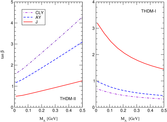
FIG. 1.: The regions (below the curves for type-II and above the curves for type-I THDM) in the $\tan\beta$ versus $M_{A}$ plane allowed by the $a_{\mu}$ data at the 95% CL. Three different curves are displayed depending whether the SM prediction is given by the CLY, AY or J calculation. There is no allowed region in this range of parameters according to the DH calculation. (Here, a two-loop calculation for the THDM contribution, cf. Appendix A, is used.)

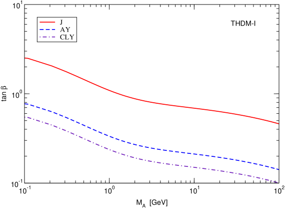
FIG. 2.: The regions (above the curves) in the $\tan\beta$ versus $M_{A}$ plane of a type-I THDM allowed by the $a_{\mu}$ data at the 95% CL. There is no allowed region in this range of parameters according to the DH calculation. (Here, a two-loop calculation for the THDM contribution, cf. Appendix A, is used.)

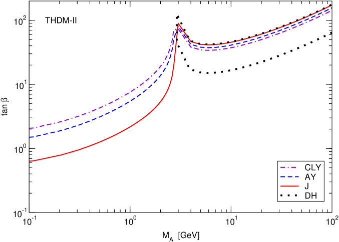
FIG. 3.: The regions in the $\tan\beta$ versus $M_{A}$ plane of a type-II THDM allowed by the $a_{\mu}$ data at the 95% CL. The allowed regions based on the calculations of CLY, AY and J are below the curves. The region allowed by the DH calculation is bounded by the dotted line. (Here, a two-loop calculation for the THDM contribution, cf. Appendix A, is used.)

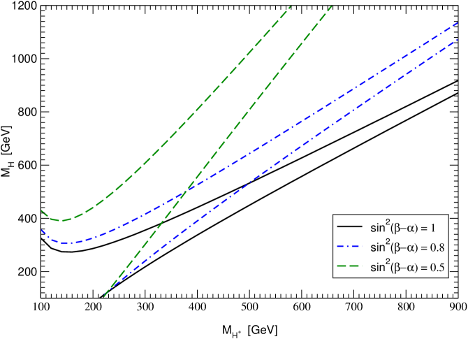
FIG. 4.: Allowed regions for $M_{H^{+}}$ vs $M_{H}$ at different values of $\sin^{2}(\beta-\alpha)$. Regions inside the solid, dot-dashed and dashed lines are allowed for $\sin^{2}(\beta-\alpha)=$ 1, 0.8 and 0.5, respectively.

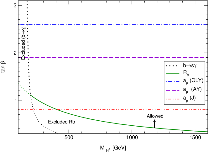
FIG. 5.: Allowed parameter region for a THDM with a light pseudoscalar $A$. The upper bounds on $\tan\beta$ derived from the $a_{\mu}$ data is for a type-II THDM with $M_{A}=0.2$ GeV. The lower bound from $R_{b}$ holds for either type-I or type-II THDM (when $\tan\beta\sim 1$). The $b\to s\gamma$ data does not provide any useful constraint for a type-I model when $\tan\beta>1$.

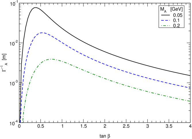
FIG. 6.: Life-time of $A$ for $M_{A}=0.05,0.1$ and $0.2$ GeV. The units have been converted from GeV^-1 to meters. The decay length of $A$ can be obtained after multiplying $1/\Gamma_{A}$ by $|{\vec{p}}|/M_{A}$, where ${\vec{p}}$ is the momentum of $A$.

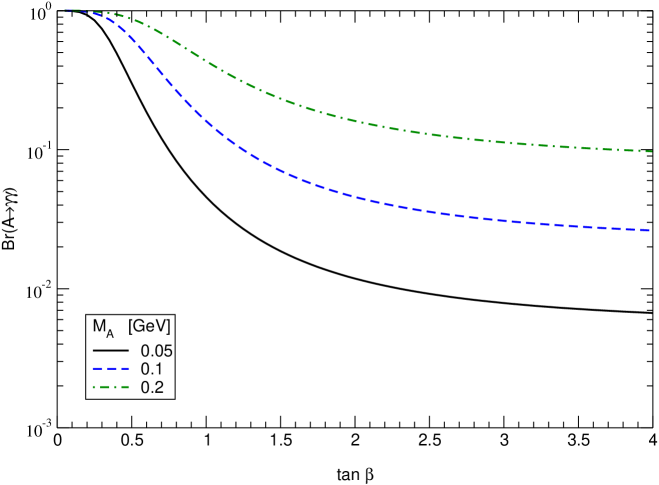
FIG. 7.: Branching ratio of $A\to\gamma\gamma$ for $M_{A}=$ 0.05, 0.1, and 0.2 GeV.

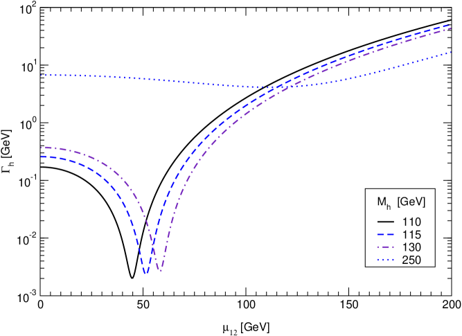
FIG. 8.: Total width of the light CP-even Higgs boson $h$ for $M_{h}=$100,115,130 and 250 GeV. This result holds for $\tan\beta=0.5$ or 2.

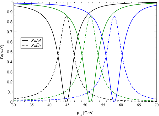
FIG. 9.: Branching ratio of $h\to AA$ and $h\to b\overline{b}$, as a function of $\mu_{12}$ for different $M_{h}$ values. From left to right: $M_{h}=$100, 115 and 130 GeV. This result holds for $\tan\beta=0.5$ or 2.

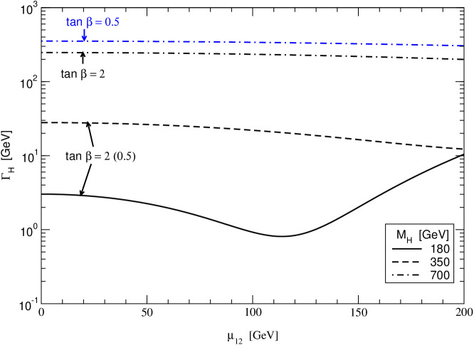
FIG. 10.: Total width of $H$ as a function of $\mu_{12}$ with $\tan\beta=0.5$ or 2, for $M_{H}=$ 180, 350 and 700 GeV.

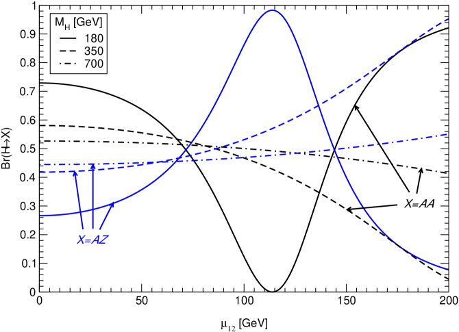
FIG. 11.: Branching ratios of $H\to AA$ and $AZ$ with $\tan\beta=2$, for $M_{H}=$ 180, 350 and 700 GeV.

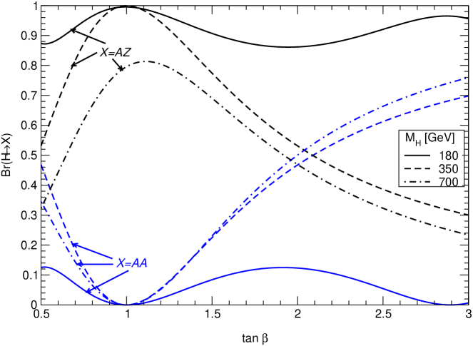
FIG. 12.: Branching ratios for $H\to AA$, and $H\to ZA$ as a function of $\tan\beta$, for $M_{H}=180$, 350 and 700 GeV with $\mu_{12}=100$ GeV.

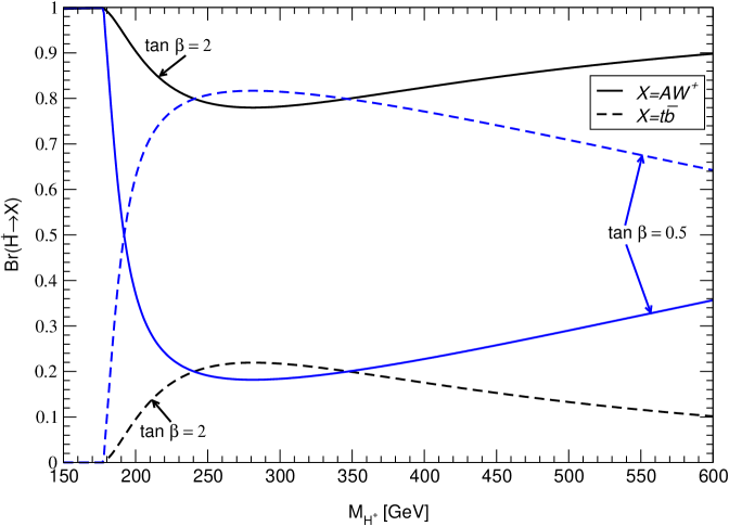
FIG. 13.: The $H^{+}\to AW^{+}$ and $H^{+}\to t\overline{b}$ branching ratios for two values of $\tan\beta$ in the type-II THDM.

FIG. 14.: Tree level diagrams for $Z\to AAA$.

FIG. 15.: Diagrams for $f{\bar{f}}\to ZAA$.

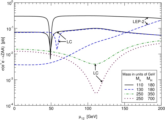
FIG. 16.: $ZAA$ production cross section at LEP-2 and LC with $\sqrt{S}=210$ GeV and 500 GeV, respectively, for a few values of $M_{h}$ and $M_{H}$ with $M_{A}=0.2$ GeV and $\tan\beta=2$.

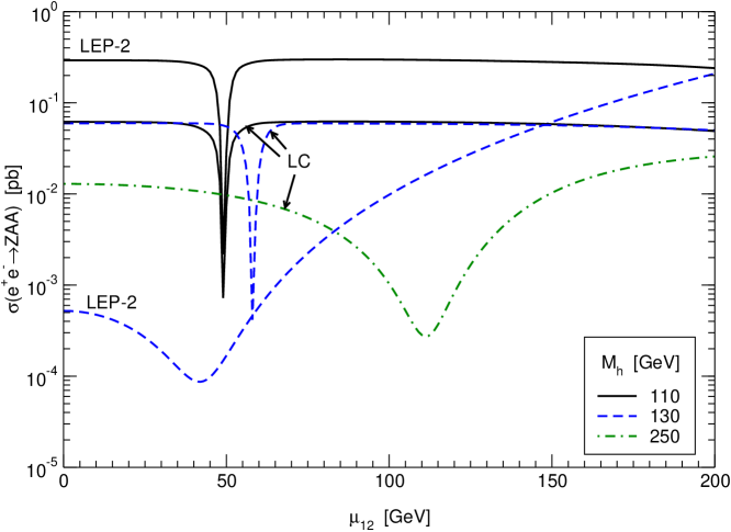
FIG. 17.: $ZAA$ production cross section at LEP-2 and LC with $\sqrt{S}=210$ GeV and 500 GeV, respectively, for a few values of $M_{h}$ with $M_{A}=0.2$ GeV, $M_{H}=1$ TeV and $\tan\beta=0.5$.

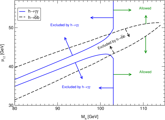
FIG. 18.: The allowed range of $\mu_{12}$ derived from the LEP-2 SM Higgs and photonic Higgs search results as a function of $M_{h}$, with $M_{A}=0.2$ GeV and $\tan\beta=0.5$. For $M_{h}<120$ GeV, this range is not sensitive to the actual value of $M_{H}$.

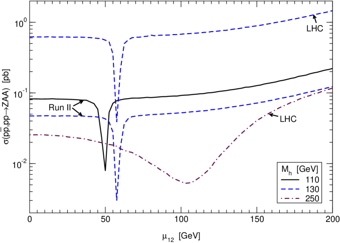
FIG. 19.: $ZAA$ production cross section at the Run-2 of the Tevatron and the LHC, for a few values of $M_{h}$, with $M_{H}=1$ TeV, $M_{A}=0.2$ GeV and $\tan\beta=0.5$.

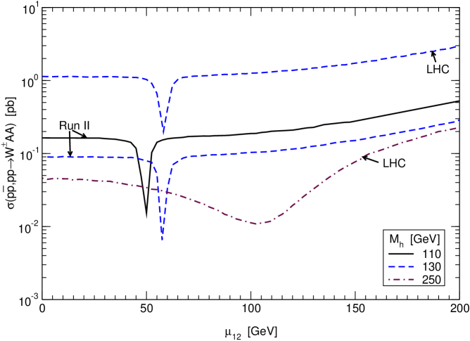
FIG. 20.: $W^{\pm}AA$ production cross section at the Run-2 of the Tevatron and the LHC, for a few values of $M_{h}$, with $M_{H^{\pm}}=1$ TeV, $M_{A}=0.2$ GeV and $\tan\beta=0.5$.

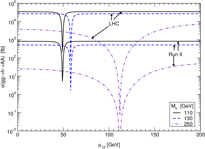
FIG. 21.: The $p{\bar{p}},pp(gg)\to h\to AA$ production cross section as a function of $\mu_{12}$ at the Tevatron Run-2 with $\sqrt{S}=2$ TeV and the LHC with $\sqrt{S}=14$ TeV, for a few values of $M_{h}$ with $M_{A}=0.2$ GeV and $\tan\beta=0.5$ or 2.

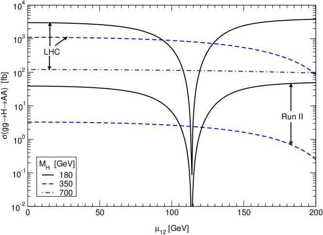
FIG. 22.: The $p{\bar{p}},pp(gg)\to H\to AA$ production cross section as a function of $\mu_{12}$ at the Tevatron Run-2 with $\sqrt{S}=2$ TeV and the LHC with $\sqrt{S}=14$ TeV, for a few values of $M_{H}$, with $M_{A}=0.2$ GeV and $\tan\beta=2$.

FIG. 23.: Contribution from the THDM to the anomalous magnetic moment of muon: neutral Higgs bosons (a), charged Higgs boson (b), and the leading two-loop contribution from the CP-odd scalar (c).

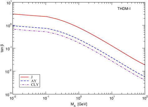
FIG. 24.: The regions (above the curves) in the $\tan\beta$ versus $M_{A}$ plane of a type-I THDM allowed by the $a_{\mu}$ data at the 95% CL, based on a one-loop calculation. There is no allowed region in this range of parameters according to the DH calculation.

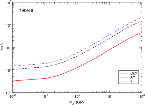
FIG. 25.: The regions (below the curves) in the $\tan\beta$ versus $M_{A}$ plane of a type-II THDM allowed by the $a_{\mu}$ data at the 95% CL, based on a one-loop calculation. There is no allowed region in this range of parameters according to the DH calculation.

FIG. 26.: Representative fermion loop diagram to the $Z\to AAA$ decay.

Constraint	Type-I THDM	Type-II THDM
$(g-2)_{\mu}$	$\tan\beta>0.4$	$\tan\beta<2.6$
($\tan\beta>1$) $b\to s\gamma$	$M_{H^{+}}>100$ GeV	$M_{H^{+}}>200$ GeV
($0.5<\tan\beta<1$) $b\to s\gamma$	—	$M_{H^{+}}>200\,-350$ GeV
($0.6<\tan\beta<1$) $R_{b}$	$M_{H^{+}}>200\,-600$ GeV	$M_{H^{+}}>200\,-600$ GeV
($\sin(\beta-\alpha)=1$) $\Delta\rho$	$M_{H}\sim M_{H^{+}}$	$M_{H}\sim M_{H^{+}}$
($\sin(\beta-\alpha)=0.8$) $\Delta\rho$	$M_{H}\sim 1.2\,M_{H^{+}}$	$M_{H}\sim 1.2\,M_{H^{+}}$
($\sin(\beta-\alpha)=0.5$) $\Delta\rho$	$M_{H}\sim 1.7\,M_{H^{+}}$	$M_{H}\sim 1.7\,M_{H^{+}}$

TABLE I.: Constraints from the low energy data for type-I and type-II models, with $M_{A}=0.2$ GeV. Here, we use the CLY calculation for the SM prediction of $a_{\mu}$. When $\sin(\beta-\alpha)$ is fixed to be 1, there is no $M_{h}$ dependence in $\rho$, otherwise, we assume $M_{h}=110$ GeV.

THDM	$C_{H}$	$C_{h}$	$C_{A}$	$C_{H^{\pm}}$
I	$\sin\alpha/\sin\beta$	$\cos\alpha/\sin\beta$	$\cot\beta$	$\cot\beta$
II	$\cos\alpha/\cos\beta$	$-\sin\alpha/\cos\beta$	$-\tan\beta$	$-\tan\beta$

TABLE II.: Higgs scalars-muon couplings in the THDM.

REFERENCES

- [1] B. Dobrescu, G. Landsberg, and K. Matchev, Phys. Rev. D 63, 075003 (2001).
- [2] D. Dobrescu, Phys. Rev. D 63, 015004 (2001).
- [3] J. F. Gunion, H. E. Haber, G. Kane, and S. Dawson, The Higgs Hunter’s Guide, (Addison Wesley, Reading, MA, 1996); hep-ph/9302272 (E).
- [4] R. Barate et al., Phys. Lett. B 487, 253 (2000); M. Acciari et al., ibid. 466, 71 (1999).
- [5] R. Barate et al., Search for a Light Higgs Boson in the Yukawa Process, Contribution to ICHEP96 Warsaw, Pol. 25-31 July 1996, PA13-027; P. Abreu et al., CERN-OPEN-99-385.
- [6] H. N. Brown, et. al., Phys. Rev. Lett. 86, 2227 (2001).
- [7] A. Csarnecki and W. J. Marciano, hep-ph/0102122.
- [8] A. Dedes and H. E. Haber, hep-ph/0102297.
- [9] F. J. Ynduráin, hep-ph/0102312.
- [10] M. Davier and A. Höcker, Phys. Lett. B 435, 427 (1998).
- [11] K. Adel and F. J. Ynduráin, hep-ph/9509378.
- [12] A. Casas, C. López and F. J. Ynduráin, Phys. Rev. D 32, 736 (1985).
- [13] W. A. Bardeen, R. Gastmans, and B. Lautrup, Nucl. Phys. B46, 319 (1972); J. P. Leveille, ibid. B137, 63 (1978); H. E. Haber, G. L. Kane, and T. Sterling, ibid. B161, 493 (1979); E. D. Carlson, S. L. Glashow, and U. Sarid, ibid. B309, 597 (1988); J. R. Primack and H. R. Quinn, Phys. Rev. D 6, 3171 (1972).
- [14] R. Barbieri and L. Maiani, Phys. Lett. B 117, 203 (1982); J. Ellis, J. S. Hagelin, and D. V. Nanopoulos, ibid. 116, 283 (1982); D. A. Kosower, L. M. Krauss, and N. Sakai, ibid. 133, 305 (1983); M. Carena, G. F. Giudice and C. E. M. Wagner, ibid. 390, 234 (1997); G.-C. Cho, K. Hagiwara, and M. Hayakawa, ibid. 478, 231 (2000); T. C. Yuan, R. Arnowitt, A. H. Chamseddine and P. Nath, Z. Phys. C 26, 407 (1984); A. Barroso, M. C. Bento, G. C. Branco, and J. C. Romao, Nucl. Phys. B250, 295 (1985); I. Vendramin, Nuovo Cimento 101 A, 731 (1989); J. A. Grifols and A. Mendez, Phys. Rev. D 26, 1809 (1982); J. L. Lopez, D. V. Nanopoulos and X. Wang, ibid. 49, 366 (1994); U. Chattopadhyay and P. Nath, ibid. 53, 1648 (1996); T. Moroi, ibid. 53, 6565 (1996); 56, 4424(E) (1997); W. Hollik, J. I. Illana, C. Schappacher, D. Stöckinger, and S. Rigolin, hep-ph/9808408; R. A. Diaz, R. Martinez and J. -Alexis Rodriguez, hep-ph/0103050.
- [15] D. Chang, W. -F. Chang, C.-H. Chou, and W.-Y. Keung, Phys. Rev. D 63, 091301 (2001).
- [16] M. Krawczyk and J. Zochowski, Phys. Rev. D 55, 6968 (1997).
- [17] P. Franzini et al., Phys. Rev. D 35, 2883 (1987). J. Lee-Franzini, in Proceedings of the XXIV International Conference on High Energy Physics, Munich, Germany, 1988, edited by R. Koffhaus and J. H. Kühn, Springer-Verlag, Berlin, 1989 p. 1432.
- [18] A. L. Kagan and M. Neubert, Eur. Phys. J. C 7, 5 (1999).
- [19] F. M. Borzumati and C. Greub, Phys. Rev. D 59, 057501 (1999); 58, 074004 (1998); hep-ph/9810240; see also, M. Ciuchini, G. Degrassi, P. Gambino, and G. F. Giudice, Nucl. Phys. B527, 21 (1998); P. Gambino, Nucl. Phys. Proc. Suppl. 86, 499 (2000); CERN-TH-2001-029.
- [20] S. Ahmed et al., hep-ex/9908022; T. E. Coan, hep-ph/0011098.
- [21] R. Barate et al., Phys. Lett. B 429, 169 (1998).
- [22] K. Abe et al., hep-ex/0103042.
- [23] H. E. Haber, in Perspectives on Higgs Physics, edited by G.L. Kane, World Scientific, Singapore, 1993, p. 79; A. Kundu and B. Mukhopadhyaya, Int. J. Mod. Phys. A 11, 5221 (1996). A. Denner, R. J. Guth, W. Hollik, and J. H. Kuhn, Z. Phys. C 51, 695 (1991). A. Djouadi, et al., Nucl. Phys. B349, 48 (1991); M. Boulware and D. Finnell, Phys. Rev. D 44, 2054 (1991). A. K. Grant, ibid. 51, 207 (1995).
- [24] H. E. Haber and H. E. Logan, Phys. Rev. D 62, 015011 (2000).
- [25] H. E. Logan, Radiative corrections to the vertex and constraints on extended Higgs sectors, PhD Thesis, hep-ph/9906332.
- [26] D. E. Groom, et al. Eur. Phys. J. C. 15 1 (2000).
- [27] P. H. Chankowski, M. Krawczyk, and J. Zochowski Eur. Phys. J. C 11, 661 (1999); G.-C. Cho and K. Hagiwara, Nuc. Phys. B574, 623 (2000); K. Hagiwara, D. Haidt, C. S. Kim, and S. Matsumoto, Z. Phys. C 64, 559 (1994); 68 352(E) (1995). T. Inami, C. S. Lim, and A. Yamada, Mod. Phys. Lett. A 7, 2789 (1992).
- [28] J. Field, Mod. Phys. Lett. A 13, 1937 (1998).
- [29] LEP Electroweak Working Group, hep-ex/0103048.
- [30] S. Kanemura, T. Kasai, and Y. Okada, Phys. Lett. B 471, 182 (1999).
- [31] A. G. Akeroyd, A. Arhrib, and E. Naimi, hep-ph/0002288; A. G. Akeroyd, Nucl. Phys. B544, 557 (1999).
- [32] A. Rosca, hep-ex/0011082; M. Aciarri et al., Phys. Lett. B 489, 115 (2000); L3 Note 2526 (2000); R. Barate et al., Phys. Lett. B 487, 241 (2000); P. Abreu et al., ibid. 507, 89 (2001).
- [33] R. Barate et al., hep-ex/0011045; P. Abreu et al., hep-ex/0011043; see also, J. Ellis, hep-ex/0011086.
- [34] H. Georgi, S. Glashow, M. Machacek, and D. V. Nanopoulos, Phys. Rev. Lett. 40 (1978) 692; A. Krause, T. Plehn, M. Spira, and P. M. Zerwas, Nucl. Phys. B519, 85 (1998); A. Djouadi, M. Spira, and P. M. Zerwas, Phys. Lett. B 264, 440 (1991); S. Dawson, Nucl. Phys. B359, 283 (1991); D. Graudenz, M. Spira, and P. M. Zerwas, Phys. Rev. Lett. 70, 1372 (1993); M. Spira, A. Djouadi, D. Graudenz, and P. M. Zerwas, Phys. Lett. B 318, 347 (1993); M. Spira, A. Djouadi, D. Graudenz, and P. M. Zerwas, Nucl. Phys. B453, 17 (1995). M. Spira, hep-ph/9711394.
- [35] E. Eichten, I. Hinchliffe, K. Lane, and C. Quigg Rev. Mod. Phys. 56, 579 (1984); ibid. 58, 1065 (1986).
- [36] L.-F. Li, in 14th International Warsaw Meeting on Elementary Particle Physics, Warsaw, Pol., 1991.
- [37] D. Chang and W.-Y. Keung, Phys. Rev. Lett. 77, 3732 (1996).
- [38] J.J. van der Bij and E.W.N. Glover, Nuc. Phys. B313, 237 (1989).
- [39] K. Cheung, C.-H. Chou, O. C. W. Kong, hep-ph/0103183; Maria Krawczyk, hep-ph/0103223.
- [40] P. Gambino and M. Misiak, hep-ph/0104034.