Relativistic quark models of baryons with instantaneous forces

Abstract

This is the first of a series of three papers treating light baryon resonances (up to 3 GeV) within a relativistically covariant quark model based on the three-fermion Bethe-Salpeter equation with instantaneous two- and three-body forces. In this paper we give a unified description of the theoretical background and demonstrate how to solve the Bethe-Salpeter equation by a reduction to the Salpeter equation. The specific new features of our covariant Salpeter model with respect to the usual nonrelativistic quark model are discussed in detail. The purely theoretical results obtained in this paper will be applied numerically to explicit quark models for light baryons in two subsequent papers Loe01b ; Loe01c .

1 Introduction

The classification of baryon resonances as three-quark states within nonrelativistic potential models has a long and very successful history. It is however unclear how to relate such models to QCD. Some ingredients of nonrelativistic quark models emerge from QCD, e.g. massive quarks as a consequence of chiral symmetry breaking, linear confinement potentials (on the lattice) due to the nonabelian gauge coupling and some candidates for spin-dependent residual interactions like one-gluon-exchange or instanton-induced quark forces. For light quark flavors it is however unclear, how to unite these features in a common picture. The main obstacle is the nonrelativistic approach which seems to be completely inadequate for small constituent quark masses and strong quark binding.

Quantum field theory seems to offer a solution to this problem, replacing the nonrelativistic wavefunctions by Bethe-Salpeter amplitudes obeying a suitable Bethe-Salpeter equation. In the case of QCD none of the basic ingredients of these equations is reliably known, i.e. we have no reliable prescription to calculate the full quark propagators and interaction vertices. Moreover we meet a serious problem with gauge invariance because the Bethe-Salpeter amplitudes are gauge-dependent. Nonetheless the general framework of quantum field theory can be used for a reasonable phenomenological description. If we want to remain as close as possible to the features of nonrelativistic quark models the Bethe-Salpeter equation should contain free quark propagators with constituent quark masses and instantaneous, unretarded interactions only. Both requirements are purely phenomenological assumptions but reasonably justified by the apparent success of nonrelativistic quark models. In this way these Bethe-Salpeter amplitudes form a more suitable basis for quark models, but respecting, in particular, relativistic covariance. As such it was already successfully used for the description of light mesons ReMu94 ; MuRe94 ; MuRe95 ; Mu96 ; MePe96 ; KoRi00 ; RiKo00 . The baryon Bethe-Salpeter equation with genuine instantaneous three-quark forces is solved as in the mesonic calculations by a reduction to a three-dimensional integral equation (Salpeter equation) which is very similar to the Schrödinger equation. The spectrum contains however also antiparticle solutions corresponding to particles with charge conjugated quantum numbers. This situation is new and needs a special discussion. Another complication arises when genuine two-particle interactions are taken into account. In quark models this is natural, when the (three-body) confinement forces are supplemented by a two-body residual interaction (one-gluon-exchange, instanton induced forces). In this case an effective three-body interaction kernel has to be derived.

None of these features is entirely new, but there is no reference in the literature which presents this theoretical background in a unified way. The purpose of this paper is to fill this gap. In two consecutive papers Loe01b ; Loe01c we will use these purely theoretical results for specific calculations of the baryon spectrum up to 3 GeV.

This paper is organized as follows: In section 2 we briefly recall how in quantum field theory bound states of three fermions occur as poles in the six-point Green’s function defining the Bethe-Salpeter amplitudes as the corresponding residua at these poles. This property of the Green’s function is used in section 3 do derive simultaneously the Bethe-Salpeter equation for the Bethe-Salpeter amplitudes and their normalization condition in a simple and appealing way by a Laurent expansion of the integral equation for the six-point Green’s function in the vicinity of this pole. Section 4 is concerned with the reduction of the full eight-dimensional Bethe-Salpeter equation to a six-dimensional Salpeter equation by integrating out the relative energy dependence of the full Bethe-Salpeter amplitudes. To this end we use a covariant formulation of the instantaneous approximation for three- and two-body interaction kernels and assume that the full quark propagators can be suitably approximated by their free forms introducing effective constituent quark masses. In a first step, taking only the genuine (instantaneous) three-body kernels into account, we show how a straightforward reduction can then be performed, thus yielding a reduced equation which may be formulated as an ordinary eigenvalue problem in Hamiltonian form, where the Hamiltonian is hermitean with respect to a scalar product induced by the normalization condition of the Salpeter amplitudes. Complications arise for the more general case when also genuine two-particle interactions are taken into account. This case needs a special discussion and we demonstrate that a reduction to a Salpeter equation in the same Hamiltonian form can nevertheless be achieved by deriving an effective instantaneous three-body kernel which parameterizes all retardation effects of the unconnected two-body interactions. In section 5 we present the Salpeter equation in Born approximation of the quasi potential which constitutes the basic covariant equation of our model. We discuss the structure and main features of the Salpeter equation and its solutions with respect to the ordinary nonrelativistic quark model. Special features discussed in this section are the one-to-one correspondence of the Salpeter amplitudes to the states of the nonrelativistic quark model and the additional anti-particle solutions of the Salpeter equation. Finally we give a summary and conclusion in section 6.

2 Green’s functions and Bethe-Salpeter amplitudes

In non-relativistic quantum mechanics, a bound state of three particles is described by a normalized wave function satisfying the three-body Schrödinger equation. This is in general the underlying equation for the description of baryons as bound states of three quarks in the framework of the various phenomenological non-relativistic potential models. A more profound basis for describing bound states in relativistic quantum field theory is the Bethe-Salpeter equation SaBe51 for the so-called Bethe-Salpeter amplitudes, which might be considered as the covariant analogues of ’wave functions’ in the non-relativistic case. The Bethe Salpeter equation has been first derived for the two-particle system by Salpeter and Bethe SaBe51 . Taylor Tay66 investigated the application of the Bethe-Salpeter equation to the three-body system.

In this section, we outline a method to treat the three fermion bound state problem in relativistic quantum field theory by using Green’s function techniques. This allows to derive the Bethe-Salpeter equation for three bound fermions simultaneously with the normalization condition of the corresponding Bethe-Salpeter amplitudes. The method is based on the fact that in general a bound state of elementary particles, whose fields appear in the underlying interaction Lagrangian, corresponds to a pole in the total energy of the Feynman propagator (Green’s function) of the many particle system. These poles do not arise from single perturbative Feynman diagrams, but rather from an infinite series of diagrams. In this context the Bethe-Salpeter amplitude is then defined as the residuum of the bound-state pole of the Green’s function. This connection between bound states and the singularities of Green’s functions was originally the basis of the first rigorous proof of the two-particle Bethe-Salpeter equation given by Gell-Mann and Low GeLo51 . However, this non-perturbative approach is clearly general and can be applied generically to the n-body Green’s function as shown for instance in the textbook of Weinberg Wein95 . As mentioned above, we apply this method to the case of three fermions (quarks) only. It consists of the following three steps Mey74 ; BoMe79 ; FlSc82 :

1. Starting point is the six-point Green’s function describing the propagation of three interacting fermions. In section 2.1 we analyze the structure of the usual perturbative power series expansion of the three-quark Feynman propagator: introducing the concept of irreducible interaction kernels for the case of three particles in a manner similar to that of Salpeter and Bethe in the two-particle case SaBe51 , we outline, how the infinite power series can be rearranged into an inhomogeneous integral equation.

2. In section 2.5 we examine the analytical structure of the six-point Green’s function: we isolate the contribution of a three-fermion bound state to the six-point Green’s function and show, how the bound state gives rise to a pole in the total energy variable (or in the invariant total four-momentum squared). This procedure defines the Bethe-Salpeter amplitudes of a specific bound state by the residue of the corresponding bound-state pole which factorizes into the Bethe-Salpeter amplitude and its adjoint.

3. Finally, by a Laurent expansion of the Green’s function in the vicinity of this bound-state pole and using the results from sects. 2.1 and 2.5, we will derive a homogeneous integral equation for bound states, i.e. the Bethe-Salpeter equation along with the normalization condition of the corresponding amplitudes. This will be done in section 3.

2.1 The six-point Green’s function for three fermions

The fundamental quantity describing three interacting fermions in quantum field theory is the six-point Greens’s function (or three-fermion Feynman propagator), which is the vacuum expectation value of a time ordered product of three fermion field operators $\Psi^{i}$ and their adjoints $\overline{\Psi}^{i}:={\Psi^{i}}^{\dagger}\gamma^{0}$ in the Heisenberg picture:

$$G_{a_{1}a_{2}a_{3};\;a^{\prime}_{1}a^{\prime}_{2}a^{\prime}_{3}}(x_{1},x_{2},x_{3};x_{1}^{\prime},x_{2}^{\prime},x_{3}^{\prime}):=$$

$$-\langle 0|\;T\;\Psi^{1}_{a_{1}}(x_{1})\Psi^{2}_{a_{2}}(x_{2})\Psi^{3}_{a_{3}}(x_{3})\overline{\Psi}^{1}_{a^{\prime}_{1}}(x^{\prime}_{1})\overline{\Psi}^{2}_{a^{\prime}_{2}}(x^{\prime}_{2})\overline{\Psi}^{3}_{a^{\prime}_{3}}(x^{\prime}_{3})|0\rangle.$$

Here the $a_{i}=(\alpha_{i},f_{i},c_{i})$ denote multi-indices combining the indices of the quark fields $\alpha_{i}$ in Dirac, $f_{i}$ in flavor and $c_{i}$ in color space. $|0\rangle$ denotes the true physical vacuum state and $T$ is the time ordering operator acting on a general $n$-fold product of Heisenberg fermion field operators $A^{i}=\Psi$ or $\overline{\Psi}$, $(i=1,\ldots,n)$ defined as

$$T\left\{A^{1}(x_{1})A^{2}(x_{2})\cdots A^{n}(x_{n})\right\}$$ (2)

$$= \textrm{sign}(\sigma)\;T\left\{A^{\sigma(1)}(x_{\sigma(1)})A^{\sigma(2)}(x_{\sigma(2)})\cdots A^{\sigma(n)}(x_{\sigma(n)})\right\}{}$$

$$:= \sum_{\sigma\in S_{n}}\textrm{sign}(\sigma)\;A^{\sigma(1)}(x_{\sigma(1)})A^{\sigma(2)}(x_{\sigma(2)})\;\cdots A^{\sigma(n)}(x_{\sigma(n)})\;\theta(x^{0}_{\sigma(1)},x^{0}_{\sigma(2)},\ldots,x^{0}_{\sigma(n)}),$$

where the sum runs over all permutations $\sigma\in S_{n}$ with signum sign$(\sigma)$. $\theta$ is a generalization of the usual Heaviside function

$$\theta(x^{0}_{1},x^{0}_{2},\ldots,x^{0}_{n})=\left\{\begin{array}[]{ll}1&\textrm{for }x^{0}_{1}\geq x^{0}_{2}\geq\cdots\geq x^{0}_{n}\\[5.69054pt] 0&\textrm{otherwise}\end{array}\right..$$ (3)

Among other possibilities (depending on the time ordering considered) the six-point Green’s function $G$ represents the probability amplitude for three (generally off-shell) quarks to propagate from space-time points $x^{\prime}_{1},x^{\prime}_{2},x^{\prime}_{3}$ to $x_{1},x_{2},x_{3}$. Using the technique of ordinary time-dependent perturbation theory, the six-point Green’s function $G$ may be expressed in the form of an infinite power series (see any standard textbook of quantum field theory, for instance Lur68 ):

$$G(x_{1},x_{2},x_{3};x_{1}^{\prime},x_{2}^{\prime},x_{3}^{\prime})=\frac{-1}{\langle 0|T\exp\left(-\textrm{i}\int_{-\infty}^{+\infty}dt\;\hat{H}_{Ip}(t)\right)|0\rangle}\sum_{k=1}^{\infty}\frac{(-\textrm{i})^{k}}{k!}\int\textrm{d}^{4}y_{1}\ldots\textrm{d}^{4}y_{k}$$ (4)

$$\qquad\times{\langle 0|T\Psi_{Ip}^{1}(x_{1})\Psi_{Ip}^{2}(x_{2})\Psi_{Ip}^{3}(x_{3})\overline{\Psi}_{Ip}^{1}(x^{\prime}_{1})\overline{\Psi}_{Ip}^{2}(x^{\prime}_{2})\overline{\Psi}_{Ip}^{3}(x^{\prime}_{3})\hat{\cal H}_{Ip}(y_{1})\ldots\hat{\cal H}_{Ip}(y_{k})|0\rangle}.$$

Now the state $|0\rangle$ represents the unperturbed vacuum and $\Psi_{Ip}$, $\bar{\Psi}_{Ip}$, $\hat{H}_{Ip}$ and $\hat{\cal H}_{Ip}$ are the field operators, the interaction Hamiltonian and the Hamiltonian density operator in the interaction picture, respectively.

2.2 The integral equation for the six-point Green’s function

Using Wick’s theorem for time ordered products of field operators, the right hand side of eq. (4) may be evaluated order by order (in the coupling constant) to obtain a power series expansion which may be represented in terms of ordinary Feynman graphs describing the interaction of two or three fermions in finite order (see fig. 1).

Figure 1: Finite order perturbative contributions to the six-point Green’s function $G$.

In scattering processes (at high energy), where neither a three-body bound state nor a two-body bound state in any of the two-particle subsystems occurs, only a finite set of diagrams may be taken into consideration. The investigation of bound states, however, requires to go beyond such a perturbative approach, i.e. an infinite sum of diagrams (or at least an infinite subset of diagrams) has to be taken into account. The reason for this is that e.g. a three-body bound state leads to a pole of the Green’s function in the total energy variable, as we will see in sect. 2.5. But such a pole never arises from a finite set of Feynman diagrams alone. To go beyond perturbation theory, one recasts the infinite power series expansion (4) in the form of an inhomogeneous integral equation, as it was done by Bethe and Salpeter SaBe51 for the case of two particles. Let us briefly sketch this procedure for the case of three fermions:

1.) One introduces the concept of irreducibility, i.e. one classifies all those diagrams appearing in the power expansion series (4) in reducible and irreducible graphs. For the definition of (ir)reducibility in the case of three interacting particles we distinguish two- and three-particle interactions:

• A connected two-fermion interaction graph is called irreducible, if it cannot be split into two simpler graphs by cutting two fermion lines only. Some examples of irreducible two-body diagrams are shown in fig. 2.

• Correspondingly, a connected three-fermion interaction is called irreducible, if it cannot be separated into two simpler graphs by just cutting three fermion lines. Examples of such graphs are given in fig. 3.

• All other interaction graphs are called reducible. Clearly, due to the above definitions of irreducibility, reducible diagrams can always be cut into irreducible parts.

2.) The (infinite) sum of all irreducible connected two-particle graphs is collected into the so-called irreducible two-particle interaction kernel

$$K^{(2)}_{a_{1}a_{2};\;a^{\prime}_{1}a^{\prime}_{2}}(x_{1},x_{2};x_{1}^{\prime},x_{2}^{\prime}).$$ (5)

See fig. 2 for a diagrammatic representation of $K^{(2)}$. Similarly, all irreducible connected three-particle graphs are added up to the so-called irreducible three-particle interaction kernel

$$K^{(3)}_{a_{1}a_{2}a_{3};\;a^{\prime}_{1}a^{\prime}_{2}a^{\prime}_{3}}(x_{1},x_{2},x_{3};x_{1}^{\prime},x_{2}^{\prime},x_{3}^{\prime}).$$ (6)

A graphical picture of $K^{(3)}$ is shown in fig. 3. The arguments $x^{\prime}_{i}$, $x_{i}$ and multi-indices $a^{\prime}_{i}$, $a_{i}$ in (5) and (6) indicate the coordinate space and the Dirac, flavor and color space dependences of the kernels, respectively.

Figure 2: Graphical representation of the two-particle irreducible Bethe-Salpeter kernel $K^{(2)}$ as sum of all possible connected irreducible two-particle interactions.

Figure 3: Diagrammatic picture of the three-particle irreducible Bethe-Salpeter kernel $K^{(3)}$ as sum of all possible connected irreducible three-particle interactions.

3.) Apart from the connected two- and three-particle interactions, applying Wick’s theorem to the right hand side of eq. (4) also generates unconnected terms, as e.g. the bare quark propagators, but moreover all kinds of self-energy contributions to the single fermion lines of each quark, summing up to the full quark propagators

$$S^{i}_{F\;a_{i}a^{\prime}_{i}}(x_{i},x^{\prime}_{i})=\langle 0|T\Psi^{i}_{a_{i}}(x_{i})\overline{\Psi}^{i}_{a^{\prime}_{i}}(x^{\prime}_{i})|0\rangle,$$ (7)

as indicated in fig. 4.

Figure 4: Perturbation series of the full dressed quark propagators defined in eq. (7).

4.) All reducible interaction diagrams of any desired order appearing in the power series expansion can now be generated by iteration of the irreducible two-particle (in each quark pair) and three-particle interaction kernels $K^{(2)}$ and $K^{(3)}$ using the full quark propagators $S_{F}^{i}$ for the inner fermion lines. This is accomplished to all orders by virtue of the following inhomogeneous integral equation, which uses the two- and three-particle interaction kernels as integral kernels Tay66 ; SaBe51 , i.e.

$$G_{a_{1}a_{2}a_{3};\;a^{\prime}_{1}a^{\prime}_{2}a^{\prime}_{3}}(x_{1},x_{2},x_{3};x_{1}^{\prime},x_{2}^{\prime},x_{3}^{\prime})=$$ (8)

$$S^{1}_{F\;a_{1}a^{\prime}_{1}}(x_{1},x^{\prime}_{1})\;S^{2}_{F\;a_{2}a^{\prime}_{2}}(x_{2},x^{\prime}_{2})\;S^{3}_{F\;a_{3}a^{\prime}_{3}}(x_{3},x^{\prime}_{3}){}$$

$$-\textrm{i}\int\textrm{d}^{4}y_{1}\;\textrm{d}^{4}y_{2}\;\textrm{d}^{4}y_{3}\;\;S^{1}_{F\;a_{1}b_{1}}(x_{1},y_{1})\;S^{2}_{F\;a_{2}b_{2}}(x_{2},y_{2})\;S^{3}_{F\;a_{3}b_{3}}(x_{3},y_{3}){}$$

$$\phantom{-i}\int\textrm{d}^{4}y_{1}^{\prime}\;\textrm{d}^{4}y_{2}^{\prime}\;\textrm{d}^{4}y_{3}^{\prime}\;\;K^{(3)}_{b_{1}b_{2}b_{3};\;b^{\prime}_{1}b^{\prime}_{2}b^{\prime}_{3}}(y_{1},y_{2},y_{3};y_{1}^{\prime},y_{2}^{\prime},y_{3}^{\prime})\;G_{b^{\prime}_{1}b^{\prime}_{2}b^{\prime}_{3};\;a^{\prime}_{1}a^{\prime}_{2}a^{\prime}_{3}}(y_{1}^{\prime},y_{2}^{\prime},y_{3}^{\prime};x_{1}^{\prime},x_{2}^{\prime},x_{3}^{\prime}){}$$

$$-\textrm{i}\sum_{cycl.Perm.\atop(123)}\int\textrm{d}^{4}y_{1}\;\textrm{d}^{4}y_{2}\;\;S^{1}_{F\;a_{1}b_{1}}(x_{1},y_{1})\;S^{2}_{F\;a_{2}b_{2}}(x_{2},y_{2}){}$$

$$\phantom{-i\sum_{cycl.Perm.\atop(123)}}\int\textrm{d}^{4}y_{1}^{\prime}\;\textrm{d}^{4}y_{2}^{\prime}\;\;K^{(2)}_{b_{1}b_{2};\;b^{\prime}_{1}b^{\prime}_{2}}(y_{1},y_{2};y_{1}^{\prime},y_{2}^{\prime})\;G_{b^{\prime}_{1}b^{\prime}_{2}a_{3};\;a^{\prime}_{1}a^{\prime}_{2}a^{\prime}_{3}}(y_{1}^{\prime},y_{2}^{\prime},x_{3};x_{1}^{\prime},x_{2}^{\prime},x_{3}^{\prime}),$$

where our notation implies summation over indices $b_{i}$, $b^{\prime}_{i}$ occurring twice. For a diagrammatic illustration of this integral equation, see fig. 5. In fact, the Neumann iteration of this integral equation reproduces all possible reducible interactions and thus precisely all the terms of the power series expansion of eq. (4).

Figure 5: Graphical illustration of the inhomogeneous integral equation 8 for the six-point Green’s function $G$. $K^{(3)}$ and $K^{(2)}$ denote the irreducible three- and two-body Bethe-Salpeter kernels, respectively, represented graphically in figs. 2 and 3. Thick arrows on quark lines indicate full dressed quark propagators as shown diagrammatically in fig. 4.

Note that also the irreducible interaction kernels $K^{(2)}$ and $K^{(3)}$ consist already of an infinite number of graphs and in general cannot be calculated exactly. They are basically unknown functions and thus have to be parameterized phenomenologically. However, the decisive advantage of the non-perturbative construction of the Green’s function $G$ from an inhomogeneous integral equation (8) is that its solution automatically implies an infinite number of interactions even if the kernels are approximated by their lowest order Born terms, which constitutes the so-called ladder approximation. Such an approximation is sufficient in theories, where the coupling constant is small and the interaction kernels may be considered as an asymptotic series expanded in terms of the (small) coupling constant. (In such a case one would expect most of the binding of a bound state to come from the repeated action of the Born diagrams alone.)

For further discussion of eq. (8) it is useful to introduce an appropriate compact notation. First let us combine the irreducible two- and three-body kernels $K^{(2)}$ and $K^{(3)}$ to a single integral kernel $K$. We introduce the inverse ${S_{F}^{k}}^{-1}$ of the full quark propagator $S_{F}^{k}$ by

$$\int\textrm{d}^{4}y_{k}\;S^{k}_{F\;a_{k}b}(x_{k},y_{k})\;{S_{F}^{k}}^{-1}_{ba^{\prime}_{k}}(y_{k},x^{\prime}_{k})=\delta_{a_{k}a^{\prime}_{k}}\;\delta^{(4)}(x_{k}-x^{\prime}_{k}).$$ (9)

This allows to rewrite the sum of the two-particle interactions $K^{(2)}$ in each quark pair in the form of a three-body kernel

$$\overline{K}^{(2)}_{a_{1}a_{2}a_{3};\;a^{\prime}_{1}a^{\prime}_{2}a^{\prime}_{3}}(x_{1},x_{2},x_{3};x_{1}^{\prime},x_{2}^{\prime},x_{3}^{\prime}):=\sum_{\footnotesize\begin{array}[]{c}(ijk)=\\ \textrm{cycl. perm. of}\\ (123)\end{array}}K^{(2)}_{a_{i}a_{j};\;a^{\prime}_{i}a^{\prime}_{j}}(x_{i},x_{j};x_{i}^{\prime},x_{j}^{\prime})\;{S_{F}^{k}}^{-1}_{a_{k}a^{\prime}_{k}}(x_{k},x_{k}^{\prime}).$$ (10)

In this form we can combine the two-body interaction kernels with the three-body kernel $K^{(3)}$ to a uniform integral kernel $K$ (see fig. 6):

$$K:=K^{(3)}+\overline{K}^{(2)}.$$ (11)

Figure 6: The integral kernel $K$ combining the three-body irreducible kernel and the two-body irreducible kernels in each quark pair; the filled circle denotes an inverse full quark propagator.

Moreover, we introduce the symbol $G_{0}$ for the triple tensor product of the single quark propagators $S_{F}^{i}$ which is the lowest order contribution to $G$:

$${G_{0\;}}_{a_{1}a_{2}a_{3};\;a^{\prime}_{1}a^{\prime}_{2}a^{\prime}_{3}}(x_{1},x_{2},x_{3};x_{1}^{\prime},x_{2}^{\prime},x_{3}^{\prime}):=S^{1}_{F\;a_{1}a^{\prime}_{1}}(x_{1},x^{\prime}_{1})\;S^{2}_{F\;a_{2}a^{\prime}_{2}}(x_{2},x^{\prime}_{2})\;S^{3}_{F\;a_{3}a^{\prime}_{3}}(x_{3},x^{\prime}_{3}).$$ (12)

Finally, we define a shorthand operator product notation for the summation over indices and the integral operation in coordinate space:

$$\left[A\;B\right]_{a_{1}a_{2}a_{3};\;a^{\prime}_{1}a^{\prime}_{2}a^{\prime}_{3}} := \sum_{b_{1}b_{2}b_{3}}A_{a_{1}a_{2}a_{3};\;b_{1}b_{2}b_{3}}\;B_{b_{1}b_{2}b_{3};\;a^{\prime}_{1}a^{\prime}_{2}a^{\prime}_{3}},$$ (13)

$$\left[A\;B\right](x_{1},x_{2},x_{3};x_{1}^{\prime},x_{2}^{\prime},x_{3}^{\prime}) := \int\textrm{d}^{4}y_{1}\textrm{d}^{4}y_{2}\textrm{d}^{4}y_{3}\;A(x_{1},x_{2},x_{3};y_{1},y_{2},y_{3})\;B(y_{1},y_{2},y_{3};x_{1}^{\prime},x_{2}^{\prime},x_{3}^{\prime}).$$ (14)

With these definitions the inhomogeneous integral equation for the six-point Green’s function can be represented in the more compact form of an operator equation

$$G=G_{0}-\textrm{i}\;G_{0}\;K\;G.$$ (15)

Note that this integral equation for the Green’s function $G$ can also be written in its equivalent adjoint form, where the operator product $G_{0}\;K\;G$ on the right hand side of eq. (15) appears in reverse order:

$$G=G_{0}-\textrm{i}\;G\;K\;G_{0}.$$ (16)

The equivalence of the integral equation (15) and its adjoint (16) is obvious, since both equations have the same Neumann series.

2.3 Space-time translational invariance

The six-point Green’s function $G$ as defined in eq. (2.1) is invariant under arbitrary space-time translations, i.e.

$$G(x_{1},x_{2},x_{3};x^{\prime}_{1},x^{\prime}_{2},x^{\prime}_{3})=G(x_{1}+a,x_{2}+a,x_{3}+a;x^{\prime}_{1}+a,x^{\prime}_{2}+a,x^{\prime}_{3}+a)$$ (17)

for all $a\in{\rm I\kern-1.99997ptR}^{4}$. Due to this symmetry it is natural to introduce new coordinates, namely an external ’center-of-mass’ coordinate $X$ and internal, i.e. translationally invariant, relative coordinates $\xi$ and $\eta$, the so-called Jacobi coordinates. We choose:

$$\begin{array}[]{ccl}X&:=&\frac{1}{3}(x_{1}+x_{2}+x_{3}),{}\\[8.53581pt] \xi&:=&x_{1}-x_{2},{}\\[8.53581pt] \eta&:=&\frac{1}{2}(x_{1}+x_{2}-2x_{3}),\end{array}\quad\Leftrightarrow\quad\begin{array}[]{ccl}x_{1}&=&X+\frac{1}{2}\xi+\frac{1}{3}\eta,{}\\[8.53581pt] x_{2}&=&X-\frac{1}{2}\xi+\frac{1}{3}\eta,{}\\[8.53581pt] x_{3}&=&X-\frac{2}{3}\eta.\end{array}$$

The space-like components ${\bf X}$, $\xi$ and $\eta$ of these variables can be interpreted in the non-relativistic limit as usual center-of-mass and relative coordinates for a system of three particles with equal mass. However, in a covariant framework this choice is a priori arbitrary and the variables $X$, $\xi$ and $\eta$ have in general no direct physical meaning. Choosing now specifically $a:=-\frac{1}{2}(X+X^{\prime})$ in eq. (17) we find that in fact the six-point Green’s function $G$ depends only on translationally invariant coordinate differences $X-X^{\prime}$, $\xi$, $\eta$, $\xi^{\prime}$ and $\eta^{\prime}$, i.e.

$$G(x_{1},x_{2},x_{3};\;x^{\prime}_{1},x^{\prime}_{2},x^{\prime}_{3})\equiv G(X-X^{\prime};\xi,\eta;\xi^{\prime},\eta^{\prime}).$$ (18)

Of course, the same holds also for the triple product $G_{0}$ of the free single quark propagators, and the translation invariance of the Green’s function $G$ necessarily implies that in particular the interaction kernels $K^{(3)}$ and $\overline{K}^{(2)}$ must by themselves be translationally invariant quantities. In momentum space space-time translation invariance is equivalent to the conservation of the total four-momentum. Consequently, as will be shown in the following subsection, the twelve-dimensional integral equations (15) for the six-point Green’s function in coordinate space and its adjoint (16) after Fourier transformation become only eight-dimensional integral equations in the momentum space representation. Due to momentum conservation, these momentum space representations depend only parametrically on the total four-momentum. To perform the Fourier transformation let us define the corresponding conjugate momenta to $X$, $\xi$ and $\eta$ which are given by the total four-momentum $P$ and the following relative four-momenta $p_{\xi}$ and $p_{\eta}$:

$$\begin{array}[]{ccl}P&:=&p_{1}+p_{2}+p_{3},{}\\[8.53581pt] p_{\xi}&:=&\frac{1}{2}(p_{1}-p_{2}),{}\\[8.53581pt] p_{\eta}&:=&\frac{1}{3}(p_{1}+p_{2}-2p_{3}),\end{array}\quad\Leftrightarrow\quad\begin{array}[]{ccl}p_{1}&=&\frac{1}{3}P+p_{\xi}+\frac{1}{2}p_{\eta},{}\\[8.53581pt] p_{2}&=&\frac{1}{3}P-p_{\xi}+\frac{1}{2}p_{\eta},{}\\[8.53581pt] p_{3}&=&\frac{1}{3}P-p_{\eta}.\end{array}$$

The new sets of coordinates (2.3) and (2.3) satisfy the condition

$$\langle p_{1},x_{1}\rangle+\langle p_{2},x_{2}\rangle+\langle p_{3},x_{3}\rangle=\langle P,X\rangle+\langle p_{\xi},\xi\rangle+\langle p_{\eta},\eta\rangle,$$ (19)

and a technical advantage of this special choice of variables is that the Jacobians of the transformations (2.3) and (2.3) are unity, i.e.

$$\left|\frac{\partial(X,\xi,\eta)}{\partial(x_{1},x_{2},x_{3})}\right|=1\quad\textrm{and}\quad\left|\frac{\partial(P,p_{\xi},p_{\eta})}{\partial(p_{1},p_{2},p_{3})}\right|=1.$$ (20)

2.4 Momentum space representation of the integral equation

For any six-point function $A=G$, $G_{0}$, $K$, ${\overline{K}}^{(2)}$ and $K^{(3)}$, i.e. the six-point Green’s function, the triple product of quark propagators or the interaction kernels, we define the Fourier transform by

$$\left[{\cal F}A\right](p_{1},p_{2},p_{3};p^{\prime}_{1},p^{\prime}_{2},p^{\prime}_{3}):=$$

$$\quad\quad\int\textrm{d}^{4}x_{1}\;\textrm{d}^{4}x_{2}\;\textrm{d}^{4}x_{3}\;e^{+\textrm{\footnotesize i}\left(\langle p_{1},x_{1}\rangle+\langle p_{2},x_{2}\rangle+\langle p_{3},x_{3}\rangle\right)}$$

$$\quad\quad\times\;\int\textrm{d}^{4}x^{\prime}_{1}\;\textrm{d}^{4}x^{\prime}_{2}\;\textrm{d}^{4}x^{\prime}_{3}\;e^{-\textrm{\footnotesize i}\left(\langle p^{\prime}_{1},x^{\prime}_{1}\rangle+\langle p^{\prime}_{2},x^{\prime}_{2}\rangle+\langle p^{\prime}_{3},x^{\prime}_{3}\rangle\right)}\;A(x_{1},x_{2},x_{3};x_{1}^{\prime},x_{2}^{\prime},x_{3}^{\prime}).$$

Using the properties (19) and (20) of the new coordinate sets, the Fourier transforms can be written in terms of relative Jacobi momenta and the total four-momenta,

$$\left[{\cal F}A\right](p_{1},p_{2},p_{3};p^{\prime}_{1},p^{\prime}_{2},p^{\prime}_{3}) = A_{P}(p_{\xi},p_{\eta};p_{\xi}^{\prime},p_{\eta}^{\prime})\;(2\pi)^{4}\delta^{(4)}(P-P^{\prime}).$$ (22)

Due to the translational invariance of the six-point functions $A$ the $\delta$-function reflects the conservation $P^{\prime}=P$ of total four-momentum. The remaining part $A_{P}$, just depending parametrically on $P$, is defined by the following Fourier transformation

$$A(x_{1},x_{2},x_{3};x_{1}^{\prime},x_{2}^{\prime},x_{3}^{\prime})=A(X-X^{\prime};\xi,\eta;\xi^{\prime},\eta^{\prime})$$ (23)

$$=: \int\frac{\textrm{d}^{4}P}{(2\pi)^{4}}\;e^{-\textrm{\footnotesize i}\langle P,X-X^{\prime}\rangle}\;\int\frac{\textrm{d}^{4}p_{\xi}}{(2\pi)^{4}}\;\frac{\textrm{d}^{4}p_{\eta}}{(2\pi)^{4}}\;e^{-\textrm{\footnotesize i}\langle p_{\xi},\xi\rangle}\;e^{-\textrm{\footnotesize i}\langle p_{\eta},\eta\rangle}\int\frac{\textrm{d}^{4}p_{\xi}^{\prime}}{(2\pi)^{4}}\;\frac{\textrm{d}^{4}p_{\eta}^{\prime}}{(2\pi)^{4}}\;e^{\textrm{\footnotesize i}\langle p_{\xi}^{\prime},\xi^{\prime}\rangle}e^{\textrm{\footnotesize i}\langle p_{\eta}^{\prime},\eta^{\prime}\rangle}\;A_{P}(p_{\xi},p_{\eta};p_{\xi}^{\prime},p_{\eta}^{\prime}),$$

which exhibits the exclusive dependence on the relative coordinates $X-X^{\prime}$, $\xi$, $\eta$, $\xi^{\prime}$ and $\eta^{\prime}$. The momentum space representation ${G_{0}}_{P}$ of the quark propagators $G_{0}$ then reads explicitly

$${G_{0}}_{P}\;(p_{\xi},p_{\eta};p_{\xi}^{\prime},p_{\eta}^{\prime}) = S_{F}^{1}\left(\mbox{$\frac{1}{3}P\!+\!p_{\xi}\!+\!\frac{1}{2}p_{\eta}$}\right)\otimes S_{F}^{2}\left(\mbox{$\frac{1}{3}P\!-\!p_{\xi}\!+\!\frac{1}{2}p_{\eta}$}\right)\otimes S_{F}^{3}\left(\mbox{$\frac{1}{3}P\!-\!p_{\eta}$}\right){}$$ (24)

$$\hskip 28.45274pt\times\;\;(2\pi)^{4}\;\delta^{(4)}(p_{\xi}-p_{\xi}^{\prime})\;\;(2\pi)^{4}\;\delta^{(4)}(p_{\eta}-p_{\eta}^{\prime}),$$

where (due to translational invariance) the Fourier transforms of the single quark propagators are defined by

$$S_{F}^{i}(x_{i},x_{i}^{\prime})=S_{F}^{i}(x_{i}-x_{i}^{\prime})=:\int\frac{\textrm{d}^{4}p_{i}}{(2\pi)^{4}}\;e^{-\textrm{\footnotesize i}\langle p_{i},x_{i}-x_{i}^{\prime}\rangle}\;S_{F}^{i}(p_{i}).$$ (25)

For the sake of completeness we should also specify the explicit form of the Fourier transform $\overline{K}^{(2)}_{P}$ of the two-particle term $\overline{K}^{(2)}$ defined in eq. (10). To this end we first have to define the Fourier transform of the two-particle interaction kernel $K^{(2)}(x_{i},x_{j};\;x^{\prime}_{i},x^{\prime}_{j})$. According to translational invariance, it is useful to introduce two-particle ’center of mass’ and relative coordinates $X_{k}$ and $\xi_{k}$ for each possible quark pair $(ij)$, i.e.

$$\begin{array}[]{lcl}X_{k}&:=&\frac{1}{2}(x_{i}+x_{j}){}\\[5.69054pt] \xi_{k}&:=&x_{i}-x_{j}\end{array}\quad\textrm{for}\;(ijk)=\textrm{cycl. perm. of}\;(123),$$

as well as their corresponding conjugate variables, the total two-particle momenta $P_{k}$ and the relative momenta $p_{\xi_{k}}$, i.e.

$$\begin{array}[]{lclclc}P_{k}&:=&p_{i}+p_{j}=\frac{2}{3}P+p_{\eta_{k}}{}\\[2.84526pt] p_{\eta_{k}}&:=&\frac{1}{3}(p_{i}+p_{j}-2p_{k}){}\\[8.53581pt] p_{\xi_{k}}&:=&\frac{1}{2}(p_{i}-p_{j})&\textrm{for}\;(ijk)=\textrm{cycl. perm. of}\;(123).\end{array}$$

Note that we have expressed $P_{k}$ by the total three-particle momentum $P$ and an additional variable $p_{\eta_{k}}$ in order to relate the sets $(P_{k},p_{\xi_{k}})$ of two-particle momenta to the set (2.3) of relative three-particle momenta $(p_{\xi},p_{\eta})=(p_{\xi_{3}},p_{\eta_{3}})$ in the case $(ijk)=(123)$ and to the equivalent cyclically permuted sets $(p_{\xi_{1}},p_{\eta_{1}})$ and $(p_{\xi_{2}},p_{\eta_{2}})$ in the cases $(ijk)=(231)$ and $(312)$, respectively. The cyclically permuted sets of the relative momenta are obtained by linear transformations of the existing set (2.3) according to

$$\left(\begin{array}[]{c}p_{\xi}\\[8.53581pt] p_{\eta}\end{array}\right)=\left(\begin{array}[]{c}p_{\xi_{3}}\\[8.53581pt] p_{\eta_{3}}\end{array}\right)=\left(\begin{array}[]{cc}-\frac{1}{2}&-\frac{3}{4}\\[8.53581pt] \phantom{-}1&-\frac{1}{2}\end{array}\right)\left(\begin{array}[]{c}p_{\xi_{1}}\\[8.53581pt] p_{\eta_{1}}\end{array}\right)=\left(\begin{array}[]{cc}-\frac{1}{2}&\phantom{-}\frac{3}{4}\\[8.53581pt] -1&-\frac{1}{2}\end{array}\right)\left(\begin{array}[]{c}p_{\xi_{2}}\\[8.53581pt] p_{\eta_{2}}\end{array}\right).$$ (26)

When $K^{(2)}$ depends on translationally invariant two-particle variables only, the Fourier transform of $K^{(2)}$ is given as

$$K^{(2)}(x_{i},x_{j};x^{\prime}_{i},x^{\prime}_{j})=K^{(2)}(X_{k}-X^{\prime}_{k};\xi_{k},\xi^{\prime}_{k})$$

$$=:\int\frac{\textrm{d}^{4}P_{k}}{(2\pi)^{4}}\;e^{-\textrm{\footnotesize i}\langle P_{k},X_{k}-X^{\prime}_{k}\rangle}\int\frac{\textrm{d}^{4}p_{\xi_{k}}}{(2\pi)^{4}}\;e^{-\textrm{\footnotesize i}\langle p_{\xi_{k}},\xi_{k}\rangle}\int\frac{\textrm{d}^{4}p^{\prime}_{\xi_{k}}}{(2\pi)^{4}}\;e^{\textrm{\footnotesize i}\langle p^{\prime}_{\xi_{k}},\xi^{\prime}_{k}\rangle}\;K_{P_{k}}^{(2)}(p_{\xi_{k}},p^{\prime}_{\xi_{k}}).$$

Using the definition (10) of $\overline{K}^{(2)}$ and the definitions (23) and (2.4) of the Fourier transforms of $\overline{K}^{(2)}$ and $K^{(2)}$, we find the following explicit form for $\overline{K}^{(2)}_{P}$:

$$\overline{K}^{(2)}_{P\;a_{1}a_{2}a_{3};\;a^{\prime}_{1}a^{\prime}_{2}a^{\prime}_{3}}(p_{\xi},p_{\eta};\;p_{\xi}^{\prime},p_{\eta}^{\prime})=$$

$$\sum_{(ijk)=\atop(123),(231),(312)}K^{(2)}_{(\frac{2}{3}P+p_{\eta_{k}})\;a_{i}a_{j};\;a^{\prime}_{i}a^{\prime}_{j}}(p_{\xi_{k}},p^{\prime}_{\xi_{k}})\;{S_{F}^{k}}^{-1}_{a_{k}a^{\prime}_{k}}\left(\mbox{$\frac{1}{3}P-p_{\eta_{k}}$}\right)\;(2\pi)^{4}\;\delta^{(4)}(p_{\eta_{k}}-p^{\prime}_{\eta_{k}}),$$

where ${S_{F}^{k}}^{-1}(p_{k})$ is the momentum space representation of the inverse of the full quark propagator defined in eq. (9), which obeys

$$\sum_{b_{k}}{S_{F}^{k}}_{a_{k}b_{k}}(p_{k})\;{S_{F}^{k}}^{-1}_{b_{k}a^{\prime}_{k}}(p_{k})=\delta_{a_{k}a^{\prime}_{k}}.$$ (29)

With definition (23) of the Fourier transforms of $G$, $G_{0}$ and $K$, the properties (19) and (20) of the Jacobi coordinates and the explicit form (24) of ${G_{0}}_{P}$, we are now in the position to write the inhomogeneous integral equation (15) for the six-point Green’s function $G$ in its momentum space representation,

$$G_{P}(p_{\xi},p_{\eta};p_{\xi}^{\prime},p_{\eta}^{\prime}) = S_{F}^{1}\left(\mbox{$\frac{1}{3}P+p_{\xi}+\frac{1}{2}p_{\eta}$}\right)\otimes S_{F}^{2}\left(\mbox{$\frac{1}{3}P-p_{\xi}+\frac{1}{2}p_{\eta}$}\right)\otimes S_{F}^{3}\left(\mbox{$\frac{1}{3}P-p_{\eta}$}\right)\;{}$$ (30)

$$\quad\quad\times\;(2\pi)^{4}\;\delta^{(4)}(p_{\xi}-p_{\xi}^{\prime})\;\;(2\pi)^{4}\;\delta^{(4)}(p_{\eta}-p_{\eta}^{\prime}){}$$

$$+\;\;S_{F}^{1}\left(\mbox{$\frac{1}{3}P+p_{\xi}+\frac{1}{2}p_{\eta}$}\right)\otimes S_{F}^{2}\left(\mbox{$\frac{1}{3}P-p_{\xi}+\frac{1}{2}p_{\eta}$}\right)\otimes S_{F}^{3}\left(\mbox{$\frac{1}{3}P-p_{\eta}$}\right){}$$

$$\quad\quad\times\;(-\textrm{i})\;\int\frac{\textrm{d}^{4}p_{\xi}^{\prime\prime}}{(2\pi)^{4}}\;\frac{\textrm{d}^{4}p_{\eta}^{\prime\prime}}{(2\pi)^{4}}\;\;K_{P}(p_{\xi},p_{\eta};p_{\xi}^{\prime\prime},p_{\eta}^{\prime\prime})\;G_{P}(p_{\xi}^{\prime\prime},p_{\eta}^{\prime\prime};p_{\xi}^{\prime},p_{\eta}^{\prime}),$$

where we suppressed the dependences on the indices using the shorthand tensor notation and the definition (13) of the operator product. Note that, due to the conservation of the total four momentum, the inhomogeneous integral equation depends only parametrically on the total four momentum $P$, while the integral operation involves only the relative momenta $p_{\xi}$ and $p_{\eta}$. Let us therefore introduce the momentum space representation of the operator product corresponding to (14) as

$$\left[A_{P}\;B_{P}\right](p_{\xi},p_{\eta};p_{\xi}^{\prime},p_{\eta}^{\prime}):=\int\frac{\textrm{d}^{4}p_{\xi}^{\prime\prime}}{(2\pi)^{4}}\;\frac{\textrm{d}^{4}p_{\eta}^{\prime\prime}}{(2\pi)^{4}}\;\;A_{P}(p_{\xi},p_{\eta};p_{\xi}^{\prime\prime},p_{\eta}^{\prime\prime})\;B_{P}(p_{\xi}^{\prime\prime},p_{\eta}^{\prime\prime};p_{\xi}^{\prime},p_{\eta}^{\prime})$$ (31)

which again allows to write the momentum space representations of the integral equation (15) and its adjoint (16) in a concise operator notation:

$$G_{P}={G_{0}}_{P}-\textrm{i}\;{G_{0}}_{P}\;K_{P}\;G_{P},$$ (32)

$$G_{P}={G_{0}}_{P}-\textrm{i}\;G_{P}\;K_{P}\;{G_{0}}_{P},$$ (33)

with the subscript $P$ indicating the parametrical dependence on the total four momentum, which becomes important in the next two sections for the investigation of bound-state contributions to $G$. Accordingly, we will evaluate eqs. (32) and (33) at the positions $P=\bar{P}$, where bound states with mass $M^{2}=\bar{P}^{2}$ occur, allowing the derivation of the bound state Bethe-Salpeter equation and the normalization condition of the corresponding amplitudes. But to this end we first have to know how the six-point Green’s function behaves at these bound-state pole positions. This is the topic of the next subsection.

2.5 Bound-state contributions – Bethe-Salpeter amplitudes

In quantum field theory bound states are related to the occurrence of poles of Green’s functions in the total energy variable $P^{0}$ or, equivalently, in the invariant four-momentum squared $P^{2}$. Here we verify this statement for the case of the six-point Green’s function $G_{P}$.

In the following we consider bound states of three quarks with (positive) mass $M$ and positive energy $\omega_{\bf P}:=\sqrt{{\bf P}^{2}+M^{2}}$. The corresponding Fock states with total four momentum $\bar{P}=(\omega_{\bf P},{\bf P})$ and mass $\bar{P}^{2}=M^{2}$ are denoted by $|\bar{P}\rangle$. They are eigenstates of the total four-momentum operator $\hat{P}=\hat{p}_{1}+\hat{p}_{2}+\hat{p}_{3}$, i.e.

$$\hat{P}\;|\bar{P}\rangle=\bar{P}\;|\bar{P}\rangle,$$ (34)

and are normalized covariantly according to

$$\langle\bar{P}|\bar{P}^{\prime}\rangle={(2\pi)}^{3}\;2\omega_{\bf P}\;\delta^{(3)}({\bf P}-{\bf P}^{\prime}).$$ (35)

The six-point Green’s function (2.1) in general describes all possible kinds of processes with three incoming and three outgoing fermions. The ’initial’ and ’final’ fermion or anti-fermion lines, however, are not yet fixed, until a particular time-ordering has been chosen. Here we are interested in the extraction of ’baryon’ contributions to $G$, i.e. real bound states of three quarks with positive energy that propagate forward in time. Therefore we shall consider those specific contributions to the six-point Green’s function $G$ which have the particular time orderings $x^{0}_{1},x^{0}_{2},x^{0}_{3}>x^{\prime 0}_{1},x^{\prime 0}_{2},x^{\prime 0}_{3}$, i.e. which contain

$$\theta\left(\min(x^{0}_{1},x^{0}_{2},x^{0}_{3})-\max({x^{\prime}}^{0}_{1},{x^{\prime}}^{0}_{2},{x^{\prime}}^{0}_{3})\right)=\cases{1\;\;\textrm{for}\;x^{0}_{1},x^{0}_{2},x^{0}_{3}>{x^{\prime}}^{0}_{1},{x^{\prime}}^{0}_{2},{x^{\prime}}^{0}_{3}\cr 0\;\;\textrm{otherwise}.}$$ (36)

Isolating this part of the Green’s function defined in eq. (2.1), we have

$$G_{a_{1}a_{2}a_{3};\;a^{\prime}_{1}a^{\prime}_{2}a^{\prime}_{3}}(x_{1},x_{2},x_{3};x_{1}^{\prime},x_{2}^{\prime},x_{3}^{\prime})=$$ (37)

$$-\langle 0|\;T\;\left\{\Psi^{1}_{a_{1}}(x_{1})\Psi^{2}_{a_{2}}(x_{2})\Psi^{3}_{a_{3}}(x_{3})\right\}\;\;T\;\left\{\overline{\Psi}^{1}_{a^{\prime}_{1}}(x^{\prime}_{1})\overline{\Psi}^{2}_{a^{\prime}_{2}}(x^{\prime}_{2})\overline{\Psi}^{3}_{a^{\prime}_{3}}(x^{\prime}_{3})\right\}|0\rangle{}$$

$$\quad\times\;\theta\left(\min(x^{0}_{1},x^{0}_{2},x^{0}_{3})-\max({x^{\prime}}^{0}_{1},{x^{\prime}}^{0}_{2},{x^{\prime}}^{0}_{3})\right){}$$

$$+\quad\textrm{other terms arising from different time-orderings}.$$

Now we can evaluate that contribution to the Green’s function which arises from three-quark bound states (34) with mass M, by inserting the complete set of the intermediate states $|\bar{P}\rangle$ in between the two time-ordered products in the matrix element (37):

$$G_{a_{1}a_{2}a_{3};\;a^{\prime}_{1}a^{\prime}_{2}a^{\prime}_{3}}(x_{1},x_{2},x_{3};x_{1}^{\prime},x_{2}^{\prime},x_{3}^{\prime})=$$ (38)

$$-\int\frac{\textrm{d}^{3}P}{(2\pi)^{3}\;2\omega_{\bf P}}\;\langle 0|\;T\;\Psi^{1}_{a_{1}}(x_{1})\Psi^{2}_{a_{2}}(x_{2})\Psi^{3}_{a_{3}}(x_{3})|\bar{P}\rangle\;\langle\bar{P}|\;T\;\overline{\Psi}^{1}_{a^{\prime}_{1}}(x^{\prime}_{1})\overline{\Psi}^{2}_{a^{\prime}_{2}}(x^{\prime}_{2})\overline{\Psi}^{3}_{a^{\prime}_{3}}(x^{\prime}_{3})|0\rangle{}$$

$$\quad\quad\times\;\theta\left(\min(x^{0}_{1},x^{0}_{2},x^{0}_{3})-\max({x^{\prime}}^{0}_{1},{x^{\prime}}^{0}_{2},{x^{\prime}}^{0}_{3})\right){}$$

$$+\quad\textrm{other terms}.$$

Here ’other terms’ now denotes the terms not only arising from other time-orderings, but also from other intermediate states.

We define the Bethe-Salpeter amplitude $\chi_{\bar{P}}$ for the bound state $|\bar{P}\rangle$ and its adjoint $\overline{\chi}_{\bar{P}}$ by the following transition amplitudes between the state $|\bar{P}\rangle$ and the vacuum $|0\rangle$,

$$\chi_{\bar{P}\;a_{1}a_{2}a_{3}}(x_{1},x_{2},x_{3}) := \langle 0|\;T\;\Psi^{1}_{a_{1}}(x_{1})\Psi^{2}_{a_{2}}(x_{2})\Psi^{3}_{a_{3}}(x_{3})\;|\bar{P}\rangle,$$ (39)

$$\overline{\chi}_{\bar{P}\;a^{\prime}_{1}a^{\prime}_{2}a^{\prime}_{3}}(x^{\prime}_{1},x^{\prime}_{2},x^{\prime}_{3}) := \langle\bar{P}|\;T\;\overline{\Psi}^{1}_{a^{\prime}_{1}}(x^{\prime}_{1})\overline{\Psi}^{2}_{a^{\prime}_{2}}(x^{\prime}_{2})\overline{\Psi}^{3}_{a^{\prime}_{3}}(x^{\prime}_{3})\;|0\rangle,$$ (40)

which appear in the bound-state contribution (38) to the Green’s function $G$. Due to translational invariance we can factorize the total momentum dependence of the Bethe-Salpeter amplitude $\chi_{\bar{P}}$ and its adjoint $\overline{\chi}_{\bar{P}}$ which contributes just by a trivial phase factor:

$$\chi_{\bar{P}}(x_{1},x_{2},x_{3}) = e^{-{\rm i}\langle\bar{P},X\rangle}\;\;\chi_{\bar{P}}(\xi,\eta){}$$ (41)

$$=: e^{-{\rm i}\langle\bar{P}X,\rangle}\;\int\frac{\textrm{d}^{4}p_{\xi}}{(2\pi)^{4}}\;\frac{\textrm{d}^{4}p_{\eta}}{(2\pi)^{4}}\;e^{-{\rm i}\langle p_{\xi},\xi\rangle}\;e^{-{\rm i}\langle p_{\eta},\eta\rangle}\;\chi_{\bar{P}}(p_{\xi},p_{\eta}),$$

$$\overline{\chi}_{\bar{P}}(x_{1}^{\prime},x_{2}^{\prime},x_{3}^{\prime}) = e^{{\rm i}\langle\bar{P},X^{\prime}\rangle}\;\;\overline{\chi}_{\bar{P}}(\xi^{\prime},\eta^{\prime}){}$$ (42)

$$=: e^{{\rm i}\langle\bar{P},X^{\prime}\rangle}\;\int\frac{\textrm{d}^{4}p_{\xi}^{\prime}}{(2\pi)^{4}}\;\frac{\textrm{d}^{4}p_{\eta}^{\prime}}{(2\pi)^{4}}\;e^{{\rm i}\langle p_{\xi}^{\prime},\xi^{\prime}\rangle}\;e^{{\rm i}\langle p_{\eta}^{\prime},\eta^{\prime}\rangle}\;\overline{\chi}_{\bar{P}}(p^{\prime}_{\xi},p^{\prime}_{\eta}).$$

Thus, we obtain translationally invariant Bethe-Salpeter amplitudes and their Fourier transforms which depend only on the internal relative coordinates $\xi$, $\eta$ and $p_{\xi}$, $p_{\eta}$, respectively.

The $\theta$-function in eq. (38), which dictates the specific time ordering $x^{0}_{1},x^{0}_{2},x^{0}_{3}>x^{\prime 0}_{1},x^{\prime 0}_{2},x^{\prime 0}_{3}$, gives rise to a pole of $G$ in the total energy variable $P^{0}$ and we finally arrive at the following Laurent expansion of $G_{P}$ in momentum space near the pole at $P^{0}=\omega_{\bf P}$:

$$G_{P}(p_{\xi},p_{\eta};p_{\xi}^{\prime},p_{\eta}^{\prime})=\frac{-\textrm{i}}{2\omega_{\bf P}}\;\frac{\chi_{\bar{P}}(p_{\xi},p_{\eta})\;\overline{\chi}_{\bar{P}}(p^{\prime}_{\xi},p^{\prime}_{\eta})}{P^{0}-\omega_{\bf P}+\textrm{i}\epsilon}+\;\textrm{regular terms for }P^{0}\rightarrow\omega_{\bf P},$$ (43)

or written covariantly

$$G_{P}(p_{\xi},p_{\eta};p_{\xi}^{\prime},p_{\eta}^{\prime})=-{\rm i}\;\frac{\chi_{\bar{P}}(p_{\xi},p_{\eta})\overline{\chi}_{\bar{P}}(p^{\prime}_{\xi},p^{\prime}_{\eta})}{P^{2}-M^{2}+{\rm i}\epsilon}+\;\textrm{regular terms for }P^{2}\rightarrow M^{2},$$ (44)

where we have introduced a six-point function $\left[\chi_{\bar{P}}\;\overline{\chi}_{\bar{P}}\right]$ by the separable product of the Bethe-Salpeter amplitudes allowing us to suppress the dependence on indices in (43) and (44):

$$\bigg{[}\chi_{\bar{P}}(p_{\xi},p_{\eta})\;\overline{\chi}_{\bar{P}}(p^{\prime}_{\xi},p^{\prime}_{\eta})\bigg{]}_{a_{1}a_{2}a_{3};\;a^{\prime}_{1}a^{\prime}_{2}a^{\prime}_{3}}:=\chi_{\bar{P}\;a_{1}a_{2}a_{3}}(p_{\xi},p_{\eta})\;\overline{\chi}_{\bar{P}\;a^{\prime}_{1}a^{\prime}_{2}a^{\prime}_{3}}(p^{\prime}_{\xi},p^{\prime}_{\eta}).$$ (45)

This typical analytical structure of the six-point Green’s function $G_{P}$ in the vicinity of the bound-state $P\approx\bar{P}$ enables us to isolate the three-fermion bound-state contributions and to extract the relevant quantity describing the bound states, namely the Bethe-Salpeter amplitude $\chi_{\bar{P}}$. In summary:

• We see that a three-fermion bound state with mass $M$ indeed gives rise to a first order pole in the total three-body energy $P^{0}$ at the bound-state energy $P^{0}\rightarrow\omega_{\bf P}=\sqrt{{\bf P}^{2}+M^{2}}$ or, equivalently, $P^{2}\rightarrow M^{2}$, $P^{0}>0$. This analytical dependence of $G_{P}$ on $P$ is a useful criterion to identify bound states. Note that it is just the Fourier transform of the $\theta$-function, due to the particular time-ordering (36), which causes this singularity.

• A further striking feature is that the Green’s function becomes separable on the mass shell of the bound state, i.e. the dependence on the relative momenta and also in the indices for the three incoming and outgoing quarks separates; the product of both parts, which corresponds to the residuum of the six-point-Green’s function at the baryon pole $P^{0}\rightarrow\omega_{\bf P}$, just defines the Bethe-Salpeter amplitude and its adjoint, see also fig. 7:

  $$\mathrm{Res}_{|_{P^{0}=\omega_{\bf P}}}G_{P\;a_{1}a_{2}a_{3};\;a^{\prime}_{1}a^{\prime}_{2}a^{\prime}_{3}}(p_{\xi},p_{\eta};p_{\xi}^{\prime},p_{\eta}^{\prime}) = \frac{-\textrm{i}}{2\omega_{\bf P}}\;\chi_{\bar{P}\;a_{1}a_{2}a_{3}}(p_{\xi},p_{\eta})\;\overline{\chi}_{\bar{P}\;a^{\prime}_{1}a^{\prime}_{2}a^{\prime}_{3}}(p^{\prime}_{\xi},p^{\prime}_{\eta}).$$ (46)

Evaluating the inhomogeneous integral equation (32) for the six-point Green’s function $G_{P}$ at the bound-state pole and using this special behavior (46) of $G_{P}$ at this pole position will allow to derive the Bethe-Salpeter equation for the Bethe-Salpeter amplitudes and the corresponding normalization condition. This will be shown in the next section.

Figure 7: The behavior of the six-point Green’s function $G$ in the vicinity of a three-quark bound-state pole of a baryon with mass $M$: Via the adjoint Bethe-Salpeter amplitude $\overline{\chi}_{\bar{P}}$ as ’vertex’ (right halved bubble) the three (off shell) quarks form a bound state (baryon), which then propagates by means of the propagator $\sim(P^{2}-M^{2}+{\rm i}\epsilon)^{-1}$ (denoted by the threefold line) and finally ’decays’ again via the ’vertex’ given by the Bethe-Salpeter amplitude $\chi_{\bar{P}}$ (left halved bubble) into three off shell quarks.

3 Bethe-Salpeter equation and normalization condition

With the results of the foregoing sections, we are now in the position to derive

• the Bethe-Salpeter equation for the Bethe-Salpeter amplitudes, which is an homogeneous integral equation describing the bound states relativistically,

• the normalization of the Bethe-Salpeter amplitudes.

This can be done simultaneously in a simple and appealing way by a Laurent expansion of the inhomogeneous integral equations (32) and (33) for the six-point Green’s function $G_{P}$ in the total energy variable $P^{0}$ around the bound state pole at $P=\bar{P}$. To this end it is convenient to bring the integral equation (32) and its adjoint (33) into the equivalent forms

$$\left[{G_{0}}_{P}^{-1}+\textrm{i}\;K_{P}\right]\;G_{P} = {\rm 1\kern-3.00003ptI},$$ (47)

$$G_{P}\;\left[{G_{0}}_{P}^{-1}+\textrm{i}\;K_{P}\right] = {\rm 1\kern-3.00003ptI},$$ (48)

where the dependence on the four momentum $P$ appears only on the left hand side. Here ${\rm 1\kern-3.00003ptI}$ is the identity for the operator product (31), which reads explicitly

$${\rm 1\kern-3.00003ptI}_{a_{1}a_{2}a_{3};\;a^{\prime}_{1}a^{\prime}_{2}a^{\prime}_{3}}(p_{\xi},p_{\eta};p_{\xi}^{\prime},p_{\eta}^{\prime}):=\delta_{a_{1}a^{\prime}_{1}}\delta_{a_{2}a^{\prime}_{2}}\delta_{a_{3}a^{\prime}_{3}}\;\;(2\pi)^{4}\;\delta^{(4)}(p_{\xi}-p_{\xi}^{\prime})\;\;(2\pi)^{4}\;\delta^{(4)}(p_{\eta}-p_{\eta}^{\prime}),$$ (49)

and the operator ${G_{0}}_{P}^{-1}$ is the inverse of ${G_{0}}_{P}$ with respect to this operator product, which thus obeys ${G_{0}}_{P}^{-1}\;G_{0}=G_{0}\;{G_{0}}_{P}^{-1}={\rm 1\kern-3.00003ptI}$. It is given by the triple product of the inverse quark propagators

$${G_{0}}_{P}^{-1}(p_{\xi},p_{\eta};p_{\xi}^{\prime},p_{\eta}^{\prime})\! = \!{S_{F}^{1}}^{-1}\!\left(\mbox{$\frac{1}{3}P+p_{\xi}+\frac{1}{2}p_{\eta}$}\right)\otimes{S_{F}^{2}}^{-1}\!\left(\mbox{$\frac{1}{3}P-p_{\xi}+\frac{1}{2}p_{\eta}$}\right)\otimes{S_{F}^{3}}^{-1}\!\left(\mbox{$\frac{1}{3}P-p_{\eta}$}\right){}$$ (50)

$$\quad\times\;\;(2\pi)^{4}\;\delta^{(4)}(p_{\xi}-p_{\xi}^{\prime})\;\;(2\pi)^{4}\;\delta^{(4)}(p_{\eta}-p_{\eta}^{\prime}).$$

Equations (47) and (48) imply that $G_{P}$ is the resolvent of a pseudo-Hamiltonian

$$H_{P}:={G_{0}}_{P}^{-1}+\textrm{i}\;K_{P},$$ (51)

i.e.

$$H_{P}\;G_{P}=G_{P}\;H_{P}={\rm 1\kern-3.00003ptI}.$$ (52)

In order to obtain an equation for the Bethe-Salpeter amplitudes and their normalization condition from (52), we use the analytical dependence of the six-point Green’s function $G_{P}$ on $P$ in the vicinity of the bound-state pole at $\bar{P}$ derived in the preceding subsection. Therefore we perform an expansion of the Green’s function $G_{P}$ and the pseudo-Hamiltonian $H_{P}$ in the variable $P^{0}$ around the bound-state energy $\omega_{\bf P}$. Due to eq. (43) we find a Laurent expansion of the Green’s function $G_{P}$ beginning with the first order singularity,

$$G_{P}=\frac{-{\rm i}}{2\omega_{\bf P}}\;\frac{\chi_{\bar{P}}\;\overline{\chi}_{\bar{P}}}{P^{0}-\omega_{\bf P}+{\rm i}\epsilon}\;+\;\frac{\partial}{\partial P^{0}}\;\left(P^{0}-\omega_{\bf P}\right)\;G_{P}\bigg{|}_{P^{0}=\omega_{\bf P}}\;+\;{\cal O}\left(P^{0}-\omega_{\bf P}\right)\;.$$ (53)

and analogously for the operator $H_{P}$ we have the Taylor series expansion

$$H_{P}=H_{\bar{P}}\;+\;\frac{\partial}{\partial P^{0}}\;H_{P}\bigg{|}_{P^{0}=\omega_{\bf P}}\left(P^{0}-\omega_{\bf P}\right)\;+\;{\cal O}\left(\left(P^{0}-\omega_{\bf P}\right)^{2}\right).$$ (54)

Inserting both expansions (53) and (54) into eq. (52) then yields the following Laurent expansion of the operator equation $H_{P}\;G_{P}={\rm 1\kern-3.00003ptI}$ up to the first order:

$$\begin{array}[]{rl|ll}&\displaystyle{-\;\frac{\rm i}{2\omega_{\bf P}}\;H_{\bar{P}}\;\left[\chi_{\bar{P}}\;\overline{\chi}_{\bar{P}}\right]\;\left(P^{0}-\omega_{\bf P}+i\epsilon\right)^{-1}}&\;\textrm{order}&-1\\[14.22636pt] &\displaystyle{+\;H_{\bar{P}}\;\left[\frac{\partial}{\partial P^{0}}\left[\left(P^{0}-\omega_{\bf P}\right)G_{P}\right]\right]_{P^{0}=\omega_{\bf P}}\;\!\!-\;\frac{\rm i}{2\omega_{\bf P}}\;\left[\frac{\partial}{\partial P^{0}}\;H_{P}\right]_{P^{0}=\omega_{\bf P}}\chi_{\bar{P}}\;\overline{\chi}_{\bar{P}}}&\;\textrm{order}&0\\[14.22636pt] &+\;\displaystyle{\mathcal{O}\left(P^{0}-\omega_{\bf P}\right)}&\;\textrm{orders}&\geq 1\\[14.22636pt] =&\displaystyle{{\rm 1\kern-3.00003ptI}}&\;\textrm{order}&0\end{array}$$ (55)

Comparing the expansion coefficients of each order in (55) we obtain simultaneously the equation for the amplitudes $\chi_{\bar{P}}$, i.e. the Bethe-Salpeter equation, and the normalization condition.

3.1 The Bethe-Salpeter equation for three bound fermions

The expansion coefficients in the Laurent series (55) of the order $(P^{0}-\omega_{\bf P})^{-1}$ yield

$$H_{\bar{P}}\;\left[\chi_{\bar{P}}\;\overline{\chi}_{\bar{P}}\right]=0.$$ (56)

Now the factorization property of the pole residue becomes crucial: due to the separability (46) of the product $\chi_{\bar{P}}\;\overline{\chi}_{\bar{P}}$ the operation (31) of $H_{P}$ acts only on the indices and relative momenta of $\chi_{\bar{P}}$, while $\overline{\chi}_{\bar{P}}$ remains unaffected, thus producing the Bethe-Salpeter equation for the Bethe-Salpeter amplitude $\chi_{\bar{P}}$:

$$H_{\bar{P}}\;\chi_{\bar{P}}=0.$$ (57)

Here the operator product of a six-point function $H_{P}$ with a three-point function $\chi_{\bar{P}}$ is defined, analogous to (31), as

$$\left[H_{\bar{P}}\;\chi_{\bar{P}}\right]_{a_{1}a_{2}a_{3}}(p_{\xi},p_{\eta}):=\int\frac{\textrm{d}^{4}p_{\xi}^{\prime}}{(2\pi)^{4}}\;\frac{\textrm{d}^{4}p_{\eta}^{\prime}}{(2\pi)^{4}}\;H_{\bar{P}\;a_{1}a_{2}a_{3};\;a^{\prime}_{1}a^{\prime}_{2}a^{\prime}_{3}}(p_{\xi},p_{\eta};\;p_{\xi}^{\prime},p_{\eta}^{\prime})\;\chi_{\bar{P}\;a^{\prime}_{1}a^{\prime}_{2}a^{\prime}_{3}}(p_{\xi}^{\prime},p_{\eta}^{\prime}).$$ (58)

In the same fashion the corresponding Laurent expansion of the adjoint equation $G_{P}H_{P}={\rm 1\kern-3.00003ptI}$ gives the adjoint Bethe-Salpeter equation for the adjoint amplitude $\overline{\chi}_{\bar{P}}$:

$$\overline{\chi}_{\bar{P}}\;H_{\bar{P}}=0.$$ (59)

Inserting definition (51) for $H_{\bar{P}}$ and multiplying by ${G_{0}}_{\bar{P}}$, we bring the Bethe-Salpeter equation and its adjoint into their more conventional form

$$\begin{array}[]{rcl}\chi_{\bar{P}}&=&-\textrm{i}\;{G_{0}}_{\bar{P}}\;K_{\bar{P}}\;\chi_{\bar{P}},\\[8.53581pt] \overline{\chi}_{\bar{P}}&=&-\textrm{i}\;\overline{\chi}_{\bar{P}}\;K_{\bar{P}}\;{G_{0}}_{\bar{P}},\end{array}\quad\textrm{with}\;\;K_{\bar{P}}=K^{(3)}_{\bar{P}}+\overline{K}^{(2)}_{\bar{P}}.$$ (60)

The three-body Bethe-Salpeter equation is a covariant eight-dimensional homogeneous integral equation in the variables $p_{\xi}=(p_{\xi}^{0},{\bf p_{\xi}})$ and $p_{\eta}=(p_{\eta}^{0},{\bf p_{\eta}})$ describing the properties of bound states. It reads explicitly:

$$\chi_{\bar{P}\;a_{1}a_{2}a_{3}}(p_{\xi},p_{\eta})=$$ (61)

$$S^{1}_{F\;a_{1}a^{\prime}_{1}}\left(\mbox{$\frac{1}{3}\bar{P}+p_{\xi}+\frac{1}{2}p_{\eta}$}\right)\;S^{2}_{F\;a_{2}a^{\prime}_{2}}\left(\mbox{$\frac{1}{3}\bar{P}-p_{\xi}+\frac{1}{2}p_{\eta}$}\right)\;S^{3}_{F\;a_{3}a^{\prime}_{3}}\left(\mbox{$\frac{1}{3}\bar{P}-p_{\eta}$}\right){}$$

$$\quad\times\;(-i)\;\int\frac{\textrm{d}^{4}p_{\xi}^{\prime}}{(2\pi)^{4}}\;\frac{\textrm{d}^{4}p_{\eta}^{\prime}}{(2\pi)^{4}}\;K^{(3)}_{\bar{P}\;a^{\prime}_{1}a^{\prime}_{2}a^{\prime}_{3};\;a^{\prime\prime}_{1}a^{\prime\prime}_{2}a^{\prime\prime}_{3}}(p_{\xi},p_{\eta};\;p_{\xi}^{\prime},p_{\eta}^{\prime})\;\chi_{\bar{P}\;a^{\prime\prime}_{1}a^{\prime\prime}_{2}a^{\prime\prime}_{3}}(p_{\xi}^{\prime},p_{\eta}^{\prime}){}$$

$$+\;S^{1}_{F\;a_{1}a^{\prime}_{1}}\left(\mbox{$\frac{1}{3}\bar{P}+p_{\xi}+\frac{1}{2}p_{\eta}$}\right)\;S^{2}_{F\;a_{2}a^{\prime}_{2}}\left(\mbox{$\frac{1}{3}\bar{P}-p_{\xi}+\frac{1}{2}p_{\eta}$}\right){}$$

$$\quad\times\;(-i)\;\int\frac{\textrm{d}^{4}p^{\prime}_{\xi}}{(2\pi)^{4}}\;K^{(2)}_{(\frac{2}{3}\bar{P}+p_{\eta})\;a^{\prime}_{1}a^{\prime}_{2};\;a^{\prime\prime}_{1}a^{\prime\prime}_{2}}(p_{\xi},p^{\prime}_{\xi})\;\chi_{\bar{P}\;a^{\prime\prime}_{1}a^{\prime\prime}_{2}a_{3}}(p_{\xi}^{\prime},p_{\eta}){}$$

$$+\;S^{1}_{F\;a_{1}a^{\prime}_{1}}\left(\mbox{$\frac{1}{3}\bar{P}+p_{\xi}+\frac{1}{2}p_{\eta}$}\right)\;S^{3}_{F\;a_{3}a^{\prime}_{3}}\left(\mbox{$\frac{1}{3}\bar{P}-p_{\eta}$}\right){}$$

$$\quad\times\;(-i)\;\int\frac{\textrm{d}^{4}p^{\prime}_{\xi_{2}}}{(2\pi)^{4}}\;K^{(2)}_{(\frac{2}{3}\bar{P}+p_{\eta_{2}})\;a^{\prime}_{1}a^{\prime}_{3};\;a^{\prime\prime}_{1}a^{\prime\prime}_{3}}(p_{\xi_{2}},p^{\prime}_{\xi_{2}})\;\chi_{\bar{P}\;a^{\prime\prime}_{1}a_{2}a^{\prime\prime}_{3}}\left(\mbox{$\!-\frac{1}{2}p^{\prime}_{\xi_{2}}+\frac{3}{4}p_{\eta_{2}}$},\mbox{$-p^{\prime}_{\xi_{2}}-\frac{1}{2}p_{\eta_{2}}$}\right){}$$

$$+\;S^{2}_{F\;a_{2}a^{\prime}_{2}}\left(\mbox{$\frac{1}{3}\bar{P}-p_{\xi}+\frac{1}{2}p_{\eta}$}\right)\;S^{3}_{F\;a_{3}a^{\prime}_{3}}\left(\mbox{$\frac{1}{3}\bar{P}-p_{\eta}$}\right){}$$

$$\quad\times\;(-i)\;\int\frac{\textrm{d}^{4}p^{\prime}_{\xi_{1}}}{(2\pi)^{4}}\;K^{(2)}_{(\frac{2}{3}\bar{P}+p_{\eta_{1}})\;a^{\prime}_{2}a^{\prime}_{3};\;a^{\prime\prime}_{2}a^{\prime\prime}_{3}}(p_{\xi_{1}},p^{\prime}_{\xi_{1}})\;\chi_{\bar{P}\;a_{1}a^{\prime\prime}_{2}a^{\prime\prime}_{3}}\left(\mbox{$\!-\frac{1}{2}p^{\prime}_{\xi_{1}}-\frac{3}{4}p_{\eta_{1}}$},\mbox{$p^{\prime}_{\xi_{1}}-\frac{1}{2}p_{\eta_{1}}$}\right).$$

Recall that the two sets $(p_{\xi_{1}},p_{\eta_{1}})$ and $(p_{\xi_{2}},p_{\eta_{2}})$ of relative momenta are related to the standard set $(p_{\xi},p_{\eta})=(p_{\xi_{3}},p_{\eta_{3}})$ by cyclic permutations of the quark momenta represented by the linear transformations (26). The Bethe-Salpeter equation is represented diagrammatically in fig. 8.

Figure 8: Graphical illustration of the three-fermion Bethe-Salpeter equation for the Bethe-Salpeter amplitude $\chi_{\bar{P}}$. $K^{(3)}$ and $K^{(2)}$ denote the irreducible three- and two-body interaction kernels, respectively. Thick arrows on quark lines indicate full quark propagators.

3.2 The normalization condition

Comparing the expansion coefficients of order $(P^{0}-\omega_{\bf P})^{0}$ in the Laurent series (55) gives

$$\;H_{\bar{P}}\;\left[\frac{\partial}{\partial P^{0}}\left[\left(P^{0}-\omega_{\bf P}\right)\;G_{P}\right]\right]_{P^{0}=\omega_{\bf P}}\;-\;\frac{\rm i}{2\omega_{\bf P}}\;\left[\frac{\partial}{\partial P^{0}}\;H_{P}\right]_{P^{0}=\omega_{\bf P}}\;\chi_{\bar{P}}\;\overline{\chi}_{\bar{P}}={\rm 1\kern-3.00003ptI}$$ (62)

which expresses the requirement that the product of $\chi_{\bar{P}}$ and $\overline{\chi}_{\bar{P}}$ is the residue of the bound-state pole in $G_{P}$. If we multiply this equation from the left hand side with the adjoint amplitude $\overline{\chi}_{\bar{P}}$, the first term in (62) vanishes according to the adjoint Bethe-Salpeter equation (59) and we find the normalization condition for the Bethe-Salpeter amplitudes Tom83

$$-{\rm i}\;\overline{\chi}_{\bar{P}}\;\bigg{[}\frac{\partial}{\partial P^{0}}\;H_{P}\bigg{]}_{P^{0}=\omega_{\bf P}}\!\chi_{\bar{P}}=2\omega_{\bf P}.$$ (63)

The full explicit expression then reads

$$-\textrm{i}\int\frac{\textrm{d}^{4}p_{\xi}^{\prime}}{(2\pi)^{4}}\;\frac{\textrm{d}^{4}p_{\eta}^{\prime}}{(2\pi)^{4}}\;\int\frac{\textrm{d}^{4}p_{\xi}}{(2\pi)^{4}}\;\frac{\textrm{d}^{4}p_{\eta}}{(2\pi)^{4}}$$

$$\overline{\chi}_{\bar{P}}(p_{\xi}^{\prime},p_{\eta}^{\prime})\;\bigg{[}\frac{\partial}{\partial P^{0}}\left({G_{0}}_{P}^{-1}(p_{\xi}^{\prime},p_{\eta}^{\prime},p_{\xi},p_{\eta})+{\rm i}K_{P}(p_{\xi}^{\prime},p_{\eta}^{\prime},p_{\xi},p_{\eta})\right)\bigg{]}_{P^{0}=\omega_{\bf P}}\;\chi_{\bar{P}}(p_{\xi},p_{\eta})\;\;=\;\;2\omega_{\bf P}.$$

A priori the normalization condition provides the correct relation between the amplitudes $\chi_{\bar{P}}$ and the six-point Green’s function $G$. But furthermore, this additional boundary condition is essential in selecting the proper solutions $\chi_{\bar{P}}$ of the three-fermion Bethe-Salpeter equation (61) thus providing a discrete spectrum $\bar{P}^{2}=M^{2}$ of bound states.

Note that the normalization condition for the amplitudes as written in the form of eq. (63) is not manifestly covariant in contrast to the Bethe-Salpeter equation. But it holds in any frame since both sides of eq. (63) transform like the time component of a four-vector, if the amplitudes transform properly under Lorentz transformations. However, we would like to remark here that the normalization (63) may also be rewritten in explicit covariant form as

$$-{\rm i}\;\overline{\chi}_{\bar{P}}\;\bigg{[}P^{\mu}\frac{\partial}{\partial P^{\mu}}\;H_{P}\bigg{]}_{P=\bar{P}}\chi_{\bar{P}}=2M^{2}.$$ (65)

For a diagrammatic illustration of eq. (65) see fig. 9.

Figure 9: The normalization condition for the Bethe-Salpeter amplitudes.The filled circles denote the inverse quark propagators, $K^{(2)}$ and $K^{(3)}$ are the irreducible two- and three-quark interaction kernels.

4 Reduction to the Salpeter equation

4.1 Motivation and general remarks

In principle, the Bethe-Salpeter equation (61) for three fermions, derived in the foregoing section, provides a suitable starting point for the covariant description of baryons as bound states of three quarks in the framework of QCD. Solving this equation for given single quark propagators $S_{F}$ and interaction kernels $K^{(2)}$ and $K^{(3)}$, the discrete spectrum of states is then determined by the normalization condition (65). However, an exact solution of the Bethe-Salpeter equation within the framework of QCD is impossible, since the quark propagator $S_{F}$ and the irreducible interaction kernels $K^{(2)}$ and $K^{(3)}$ are only formally defined in perturbation theory as an infinite sum of Feynman diagrams. Moreover it is unclear, which particular approximation will provide quark confinement in hadrons.

But even if the exact kernels and propagators were known in QCD, the dependence on the relative energy (or the corresponding relative time) variables leads to a complicated analytic pole structure, which so far could be treated rigorously only in the case of two scalar particles interacting through a (massless) scalar exchange (the so-called Wick-Cutkosky model, see Wi54 ; Cu54 ). Thus, the use of general two-quark and three-quark interaction kernels, that depend on the relative energy variables, leads to serious conceptional and practical problems. To our knowledge the only attempt to solve (approximately) a full four-dimensional three-quark Bethe-Salpeter equation in Euclidean space has been performed by Meyer and Böhm Mey74 ; Mey75 ; BoMe79 and subsequently by Kielanowski Kie80 and Falkensteiner Falk82 in an approach where baryons were considered as extremely strongly bound systems of three quite heavy constituent quarks $m\gg 1GeV$, that interact via harmonic oscillator interactions, so that a solution can be obtained by an expansion in powers of $\frac{1}{m}$. However, from a modern point of view, the crude approximations and especially the large constituent quark masses are questionable and not suited for phenomenologically successful applications.

Thus, the use of the full eight-dimensional Bethe-Salpeter equation is of rather limited practical value and the lack of a confinement kernel that could be rigorously derived from QCD anyhow requires an appropriate phenomenological parameterization: so far, the only ansatz that can give a realistic description of the quark confinement and thus can account for the gross features of the whole baryon spectrum up to highest orbital excitations, is the nonrelativistic quark model, which uses static two- and three-quark potentials.

For these reasons we will not treat the full three-quark Bethe-Salpeter equation. Instead we try to eliminate the difficult relative energy dependence in order to get a six-dimensional reduction of the full eight-dimensional Bethe-Salpeter equation, the so-called Salpeter equation Sa52 , with the aim to obtain a framework that is still covariant. At the same time we want to keep as close as possible to the quite successful nonrelativistic quark potential model in order to obtain at least this model as a non-relativistic limit. In this spirit, a covariant quark model for mesons based on the instantaneous $q\bar{q}$-Bethe-Salpeter equation has been developed already and has been successfully applied to the calculation of mass spectra and various transition matrix elements up to high momentum transfers, see ReMu94 ; MuRe94 . To extend this model for calculations of baryons, we make the same simplifying assumptions and approximations in the three-quark Bethe-Salpeter equation (sect. 4.2): The full quark propagators $S_{F}$ are assumed to be given by their free forms with effective constituent quark masses. Moreover, the kernels $K^{(2)}$ and $K^{(3)}$ are approximated by effective interactions that are instantaneous in the rest frame of the bound state, which thus corresponds to the neglect of retardation effects. We should mention here that the instantaneous approximation can be formulated in a frame independent way WaMa89 , so that formal covariance is preserved, which becomes important for the calculation of transitions between baryon states, where at least one of the baryon has to be boosted.

In the meson case these approximations allow for a direct and straightforward reduction to the $q\bar{q}$-Salpeter equation Sa52 ; ReMu94 ; MuRe94 by an analytical integration over the relative energy variable, since the connected instantaneous $q\bar{q}$-kernel cuts the whole relative energy dependence of the Bethe-Salpeter equation. The same applies also to the three-quark Bethe-Salpeter equation, if only an instantaneous, connected three-quark kernel $K^{(3)}$ is taken into account and two-particle kernels are neglected ($K^{(2)}=0$). In this case the Salpeter equation can be formulated in a concise Hamiltonian form with some characteristic projector properties that reduce the number of independent functions necessary to describe a baryon state. For the sake of conceptual simplicity such an approach has been used in our former investigations Met97a ; Met99a ; Met99b , where all kinds of interactions have been parameterized in a kind of collective instantaneous three-body kernel. In section 4.3 we will first give a summary of the reduction procedure in this simple and instructive case and discuss the specific structure of the resulting Salpeter equation.

However, as soon as genuine two-quark kernels $K^{(2)}$ are considered, new difficulties arise since the two-body terms are unconnected within the three-quark system: despite an instantaneous approximation of $K^{(2)}$ there remains a relative energy dependence due to retardation effects of the third non-interacting spectator quark, which is off-shell in general. In this respect the elimination of the relative energies is technically and conceptually much more involved and an enhanced reduction procedure is needed. In section 4.4 we give a procedure that nevertheless allows for the reduction to a Salpeter equation. The crucial point is the existence of a genuine instantaneous connected part of the interaction $K^{(3)}$, right from start. In our model this part will be given by a convenient form of a static three-body confinement potential that must be present for all baryon states in all sectors due to the confinement hypothesis. Recasting the Bethe-Salpeter equation into a more convenient form with all two-particle effects collected into a six-point Green’s function thus provides a similar reduction procedure as in the case of vanishing two-body interactions. Extending a kind of quasi-potential approach as it was first proposed by Logunov and Tavkhelidze LoTa63 for the equal-time Green’s function of two scalar particles, all effects of the unconnected two-body interactions can then be transformed into an effective instantaneous potential that adds to the genuine three-body kernel $K^{(3)}$ and we finally end up with a reduced equation that exhibits the same expedient projector structure as in the case where the dynamics of the quarks is given by an instantaneous three-body kernel alone. The effective potential, however, consists of an infinite perturbation series of time-ordered Feynman diagrams, which needs to be truncated for explicit calculations. In the subsequent sect. 5 we will analyze the structure of the resulting baryon Salpeter equation and its corresponding Salpeter amplitudes in detail: a remarkable substantial property of our covariant Salpeter approach will turn out to be that it exhibits a one-to-one correspondence with the states of the nonrelativistic quark model.

4.2 Approximations

In order to transform the Bethe-Salpeter equation into a solvable integral equation several simplifying approximations have to be made. To start, we follow the prescription of ReMu94 and assume free quark propagators and instantaneous interaction kernels.

4.2.1 Free quark propagators

First, we make the assumption that the full quark propagators can be approximated by the usual free fermion propagators with effective constituent quark masses $m_{i}$ for each quark

$$S^{i}_{F}\left(p_{i}\right)\approx\frac{\rm i}{\not p_{i}-m_{i}+{\rm i}\epsilon}.$$ (66)

This approximation is consistent with the picture of a hadron mainly built out of constituent quarks analogous to the non-relativistic quark model. The effective constituent quark masses $m_{i}$ enter as free parameters in our model.

4.2.2 Instantaneous approximation

Moreover, we choose the irreducible two- and three-body interaction kernels to be instantaneous in the rest frame of the baryon, meaning that in the center-of-mass system there is no dependence on the relative energy variables $p_{\xi}^{0}$ and $p_{\eta}^{0}$:

$$K^{(3)}_{P}(p_{\xi},p_{\eta};\;p_{\xi}^{\prime},p_{\eta}^{\prime})\bigg{|}_{P=(M,{\bf 0})} \stackrel{{\scriptstyle!}}{{=}} V^{(3)}({\bf p_{\xi}},{\bf p_{\eta}};\;{\bf p_{\xi}^{\prime}},{\bf p_{\eta}^{\prime}}),$$ (67)

$$K^{(2)}_{(\frac{2}{3}P+p_{\eta_{k}})}(p_{\xi_{k}},p^{\prime}_{\xi_{k}})\bigg{|}_{P=(M,{\bf 0})} \stackrel{{\scriptstyle!}}{{=}} V^{(2)}({{\bf p}_{\xi_{k}}},{{\bf p}_{\xi_{k}}^{\prime}}).$$ (68)

This approximation corresponds to the neglect of retardation effects in the rest-frame. To preserve the formal covariance of the Bethe-Salpeter equation, however, we need a covariant description of the instantaneous approximation which holds in any arbitrary reference frame of the bound state. We follow an idea of Wallace and Mandelzweig WaMa89 and introduce for arbitrary time-like total four-momenta $P$, $P^{2}>0$, the following covariant decomposition of any four-dimensional four-vector $p$,

$$p=p_{\|}\;\frac{P}{\sqrt{P^{2}}}+p_{\bot}$$ (69)

into components parallel and perpendicular to the total four-momentum $P$:

$$p_{\|}:=\frac{\langle p,P\rangle}{\sqrt{P^{2}}},\quad p_{\bot}:=p-\frac{\langle p,P\rangle}{P^{2}}\;P.$$ (70)

This is a decomposition into a time-like vector $p_{\|}\;P/\sqrt{P^{2}}$ and a space-like vector $p_{\bot}$ which effectively is three-dimensional in content. Now the instantaneous approximation, which has been formulated in eqs. (67) and (68) within the center-of-mass frame of the three-body system, can be formulated in any reference frame (which is specified by the four-momentum $P$): we assume that the kernels do not depend on the time-like parallel components of the relative momenta, i.e. ${p_{\xi}}_{\|},{p_{\eta}}_{\|},{p_{\xi}^{\prime}}_{\|},{p_{\eta}^{\prime}}_{\|}$, but only on the space-like perpendicular components:

$$K^{(3)}_{P}(p_{\xi},p_{\eta};\;p_{\xi}^{\prime},p_{\eta}^{\prime}) \stackrel{{\scriptstyle!}}{{=}} V^{(3)}({p_{\xi}}_{\bot},{p_{\eta}}_{\bot};\;{p_{\xi}^{\prime}}_{\bot},{p_{\eta}^{\prime}}_{\bot}),$$ (71)

$$K^{(2)}_{(\frac{2}{3}P+p_{\eta_{k}})}(p_{\xi_{k}},p^{\prime}_{\xi_{k}}) \stackrel{{\scriptstyle!}}{{=}} V^{(2)}({p_{\xi_{k}}}_{\bot},{p_{\xi_{k}}^{\prime}}_{\bot}).$$ (72)

For interaction kernels of this type we have

$$P^{\mu}\frac{\partial}{\partial P^{\mu}}K^{(3)}_{P}(p_{\xi},p_{\eta};\;p_{\xi}^{\prime},p_{\eta}^{\prime})\bigg{|}_{P=\bar{P}} = P^{\mu}\frac{\rm d}{{\rm d}P^{\mu}}\;V^{(3)}({p_{\xi}}_{\bot},{p_{\eta}}_{\bot};\;{p_{\xi}^{\prime}}_{\bot},{p_{\eta}^{\prime}}_{\bot})\bigg{|}_{P=\bar{P}}=0,$$ (73)

$$P^{\mu}\frac{\partial}{\partial P^{\mu}}K^{(2)}_{(\frac{2}{3}P+p_{\eta_{k}})}(p_{\xi_{k}},p^{\prime}_{\xi_{k}})\bigg{|}_{P=\bar{P}} = P^{\mu}\frac{\rm d}{{\rm d}P^{\mu}}\;V^{(2)}({p_{\xi_{k}}}_{\bot},{p_{\xi_{k}}^{\prime}}_{\bot})\bigg{|}_{P=\bar{P}}=0$$ (74)

and, consequently, these give no direct contributions to the normalization condition (65) for the Bethe-Salpeter amplitudes. In the rest frame of the baryon where $P=\bar{P}=(M,{\bf 0})$ we find

$$p_{\|}=p^{0}\qquad{\rm and}\qquad p_{\bot}=(0,{\bf p}),$$ (75)

so that the covariant formulation of the instantaneous approximation given in (71) and (72) indeed recovers the conditions (67) and (68) in the center-of-mass frame.

In the two-fermion case ReMu94 it was shown that the assumptions of free quark propagators and instantaneous interaction kernels are sufficient to completely eliminate the dependence on the relative energy dependence in order to arrive at a reduced equation which can be solved with standard techniques. In the three-fermion problem, however, this is in general not possible, unless we consider systems without two-body interactions. In the more general case new difficulties arise from the property of the two-body terms that these are unconnected within the three-body system. Despite the instantaneous approximation of the two-particle interactions, the kernel $\overline{K}^{(2)}_{P=(M,{\bf 0})}$ defined by eq. (2.4) remains retarded, since (in the CMS) it maintains the dependence on the relative energies $p_{\xi}^{0}$ and $p_{\eta}^{0}$ due to retardation effects of the third noninteracting spectator quark which is off-shell in general. Accordingly, in $\overline{K}^{(2)}_{P=(M,{\bf 0})}$ this remaining relative energy dependence is given explicitly by the inverse single quark propagator of the spectator together with its four-momentum conserving $\delta$-function:

$$\overline{K}^{(2)}_{P}(p_{\xi},p_{\eta};\;p_{\xi}^{\prime},p_{\eta}^{\prime})\bigg{|}_{P=(M,{\bf 0})}=$$ (76)

$$\sum_{{\rm cycl.perm}\atop{{\rm of}(123)}}V^{(2)}({{\bf p}_{\xi_{3}}},{{\bf p}_{\xi_{3}}^{\prime}})\otimes{S_{F}^{3}}^{-1}\left(\mbox{$\frac{1}{3}P-p_{\eta_{3}}$}\right)\bigg{|}_{P=(M,{\bf 0})}\;(2\pi)^{4}\;\delta^{(4)}(p_{\eta_{3}}-p^{\prime}_{\eta_{3}}).$$

Thus, the consideration of unconnected two-particle terms in the three-body Bethe-Salpeter equation makes a reduction technically much more involved, despite the instantaneous approximation of the two-body kernels. With regard to the goal of finding a convenient reduction procedure it is therefore instructive to consider first the conceptually much easier case of vanishing two-particle kernels, where the dynamics of the quarks is determined by a connected instantaneous three-body kernel alone. In this case the reduction of the eight-dimensional Bethe-Salpeter equation to an equivalent six-dimensional equation – the so-called Salpeter equation – is straightforward (as in the two-fermion case with a connected instantaneous two-body kernel ReMu94 ).

4.3 The reduction without two-particle kernels

Neglecting the irreducible two-particle interaction kernels, i.e. $K^{(2)}=0$, and taking only an instantaneous three-body kernel (71) into account, the Bethe-Salpeter equation and its adjoint in the center-of-mass frame of the baryon with $\bar{P}=(M,{\bf 0})\equiv M$ are given by

$$\chi_{M} = -\textrm{i}\;{G_{0}}_{M}\;V^{(3)}\;\chi_{M},$$ (77)

$$\overline{\chi}_{M} = -\textrm{i}\;\overline{\chi}_{M}\;V^{(3)}\;{G_{0}}_{M}.$$ (78)

The crucial point is now that $V^{(3)}$ being instantaneous truncates the $p_{\xi}^{0}$, $p_{\eta}^{0}$ dependences of the Bethe-Salpeter equations (77) and (78). This has the following consequences:

1.) The $p_{\xi}^{0}$, $p_{\eta}^{0}$ integration within the operator product $V^{(3)}\;\chi_{M}$ on the right hand side of eq. (77) acts on $\chi_{M}$ directly and thus can be used to reduce this eight-dimensional Bethe-Salpeter amplitude to a six-dimensional amplitude $\Phi_{M}$, i.e. in detail

$$\left[V^{(3)}\;\chi_{M}\right]({p_{\xi}},{p_{\eta}}) = \int\frac{\textrm{d}^{4}p_{\xi}^{\prime}}{(2\pi)^{4}}\;\frac{\textrm{d}^{4}p_{\eta}^{\prime}}{(2\pi)^{4}}\;V^{(3)}({\bf p_{\xi}},{\bf p_{\eta}};\;{\bf p_{\xi}^{\prime}},{\bf p_{\eta}^{\prime}})\;\chi_{M}(p_{\xi}^{\prime},p_{\eta}^{\prime}){}$$ (79)

$$= \int\frac{\textrm{d}^{3}p_{\xi}^{\prime}}{(2\pi)^{3}}\;\frac{\textrm{d}^{3}p_{\eta}^{\prime}}{(2\pi)^{3}}\;V^{(3)}({\bf p_{\xi}},{\bf p_{\eta}};\;{\bf p_{\xi}^{\prime}},{\bf p_{\eta}^{\prime}})\;\int\frac{\textrm{d}{p_{\xi}^{\prime}}^{0}}{2\pi}\;\frac{\textrm{d}{p_{\eta}^{\prime}}^{0}}{2\pi}\;\chi_{M}(p_{\xi}^{\prime},p_{\eta}^{\prime}){}$$

$$= \int\frac{\textrm{d}^{3}p_{\xi}^{\prime}}{(2\pi)^{3}}\;\frac{\textrm{d}^{3}p_{\eta}^{\prime}}{(2\pi)^{3}}\;V^{(3)}({\bf p_{\xi}},{\bf p_{\eta}};\;{\bf p_{\xi}^{\prime}},{\bf p_{\eta}^{\prime}})\;\Phi_{M}({\bf p_{\xi}^{\prime}},{\bf p_{\eta}^{\prime}}){}$$

$$= \left[V^{(3)}\;\Phi_{M}\right]({\bf p_{\xi}},{\bf p_{\eta}}).$$

Consequently, there remains a six-dimensional integral operation of $V^{(3)}$ on the reduced six-dimensional amplitude $\Phi_{M}$, which is the so-called Salpeter amplitude:

$$\Phi_{M}({\bf p_{\xi}},{\bf p_{\eta}}):=\int\frac{\textrm{d}p_{\xi}^{0}}{2\pi}\;\frac{\textrm{d}p_{\eta}^{0}}{2\pi}\;\chi_{M}\left((p_{\xi}^{0},{\bf p_{\xi}}),(p_{\eta}^{0},{\bf p_{\eta}})\right).$$ (80)

In the same way one proceeds with the operator product $\overline{\chi}_{M}\;V^{(3)}$ in the adjoint Bethe-Salpeter equation (78), i.e.

$$\left[\overline{\chi}_{M}\;V^{(3)}\right]({p_{\xi}},{p_{\eta}}) = \left[\overline{\Phi}_{M}\;V^{(3)}\right]({\bf p_{\xi}},{\bf p_{\eta}}),$$ (81)

which accordingly defines the adjoint Salpeter amplitude

$$\overline{\Phi}_{M}({\bf p_{\xi}},{\bf p_{\eta}}):=\int\frac{\textrm{d}p_{\xi}^{0}}{2\pi}\;\frac{\textrm{d}p_{\eta}^{0}}{2\pi}\;\overline{\chi}_{M}\left((p_{\xi}^{0},{\bf p_{\xi}}),(p_{\eta}^{0},{\bf p_{\eta}})\right).$$ (82)

2.) Inserting (79) and (81) into the Bethe-Salpeter equations (77) and (78), respectively, we have

$$\chi_{M} = -\textrm{i}\;{G_{0}}_{M}\;V^{(3)}\;\Phi_{M},$$ (83)

$$\overline{\chi}_{M} = -\textrm{i}\;\overline{\Phi}_{M}\;V^{(3)}\;{G_{0}}_{M},$$ (84)

which gives a prescription how to reconstruct the full Bethe-Salpeter amplitudes from the Salpeter amplitudes for any on-shell total momentum. Consequently, in the instantaneous approximation it is sufficient to know the reduced six-dimensional Salpeter amplitudes $\Phi_{M}$ and $\overline{\Phi}_{M}$ to get the full eight-dimensional Bethe-Salpeter amplitudes $\chi_{M}$ and $\overline{\chi}_{M}$, i.e. the solutions of the Bethe-Salpeter equation (77) and (78), respectively. The next step is to get an equation which determines $\Phi_{M}$ and $\overline{\Phi}_{M}$.

3.) As shown in eqs. (79) and (81), the quantities

$$\begin{array}[]{c}\Gamma_{M}({p_{\xi}},{p_{\eta}}):=\left[{G_{0}}_{M}^{-1}\;\chi_{M}\right]({p_{\xi}},{p_{\eta}})=\left[V^{(3)}\;\chi_{M}\right]({p_{\xi}},{p_{\eta}})=\left[V^{(3)}\;\Phi_{M}\right]({\bf p_{\xi}},{\bf p_{\eta}})\equiv\Gamma_{M}({\bf p_{\xi}},{\bf p_{\eta}}),\\[5.69054pt] \overline{\Gamma}_{M}({p_{\xi}},{p_{\eta}}):=\left[\overline{\chi}_{M}\;{G_{0}}_{M}^{-1}\right]({p_{\xi}},{p_{\eta}})=\left[\overline{\chi}_{M}\;V^{(3)}\right]({p_{\xi}},{p_{\eta}})=\left[\Phi_{M}\;V^{(3)}\right]({\bf p_{\xi}},{\bf p_{\eta}})\equiv\overline{\Gamma}_{M}({\bf p_{\xi}},{\bf p_{\eta}}),\end{array}$$ (85)

which are usually called amputated Bethe-Salpeter amplitudes or three-quark vertex functions, do not depend on the relative energies ${p_{\xi}}^{0}$ and ${p_{\eta}}^{0}$ in the center-of-mass frame of the baryon. Consequently, the analytical dependence of the Bethe-Salpeter amplitudes $\chi_{M}={G_{0}}_{M}\;\Gamma_{M}$ and $\overline{\chi}_{M}=\overline{\Gamma}_{M}\;{G_{0}}_{M}$ on the variables ${p_{\xi}}^{0}$ and ${p_{\eta}}^{0}$ stems exclusively from the triple tensor product ${G_{0}}_{M}$ of the free quark propagators. This enables us to reduce the eight-dimensional Bethe-Salpeter equations for the Bethe-Salpeter amplitudes to six-dimensional integral equations for the Salpeter amplitudes by integrating out the ${p_{\xi}}^{0}$, ${p_{\eta}}^{0}$ dependence on both sides of eqs. (83) and (84). The Bethe-Salpeter amplitudes on the left hand side reduce to the corresponding Salpeter amplitudes and on the right hand side the relative energy integration affects merely the free propagator ${G_{0}}_{M}$, i.e. in detail

$$\Phi_{M}({\bf p_{\xi}},{\bf p_{\eta}})=\int\frac{\textrm{d}p_{\xi}^{0}}{2\pi}\;\frac{\textrm{d}p_{\eta}^{0}}{2\pi}\;\chi_{M}\left((p_{\xi}^{0},{\bf p_{\xi}}),(p_{\eta}^{0},{\bf p_{\eta}})\right)$$ (86)

$$= -\textrm{i}\;\int\frac{\textrm{d}p_{\xi}^{0}}{2\pi}\;\frac{\textrm{d}p_{\eta}^{0}}{2\pi}\;\int\frac{\textrm{d}^{4}p_{\xi}^{\prime}}{(2\pi)^{4}}\;\frac{\textrm{d}^{4}p_{\eta}^{\prime}}{(2\pi)^{4}}\;{G_{0}}_{M}(p_{\xi},p_{\eta};\;p_{\xi}^{\prime},p_{\eta}^{\prime})\;\left[V^{(3)}\;\Phi_{M}\right]({\bf p_{\xi}^{\prime}},{\bf p_{\eta}}^{\prime}){}$$

$$= -\textrm{i}\;\int\frac{\textrm{d}^{3}p_{\xi}^{\prime}}{(2\pi)^{3}}\;\frac{\textrm{d}^{3}p_{\eta}^{\prime}}{(2\pi)^{3}}\;\int\frac{\textrm{d}p_{\xi}^{0}}{2\pi}\;\frac{\textrm{d}p_{\eta}^{0}}{2\pi}\;\int\frac{\textrm{d}p_{\xi}^{\prime 0}}{2\pi}\;\frac{\textrm{d}p_{\eta}^{\prime 0}}{2\pi}\;{G_{0}}_{M}(p_{\xi},p_{\eta};\;p_{\xi}^{\prime},p_{\eta}^{\prime})\;\left[V^{(3)}\;\Phi_{M}\right]({\bf p_{\xi}^{\prime}},{\bf p_{\eta}}^{\prime}){}$$

$$= -\textrm{i}\;\int\frac{\textrm{d}^{3}p_{\xi}^{\prime}}{(2\pi)^{3}}\;\frac{\textrm{d}^{3}p_{\eta}^{\prime}}{(2\pi)^{3}}\;\langle{G_{0}}_{M}\rangle({\bf p_{\xi}},{\bf p_{\eta}};\;{\bf p_{\xi}^{\prime}},{\bf p_{\eta}^{\prime}})\;\left[V^{(3)}\;\Phi_{M}\right]({\bf p_{\xi}^{\prime}},{\bf p_{\eta}}^{\prime}){}$$

$$= -\textrm{i}\;\left[\left\langle{G_{0}}_{M}\right\rangle\;V^{(3)}\;\Phi_{M}\right]({\bf p_{\xi}},{\bf p_{\eta}}).$$

Thus, we end up with the so-called Salpeter equation and its adjoint for the Salpeter amplitudes $\Phi_{M}$ and $\overline{\Phi}_{M}$

$$\Phi_{M} = -\textrm{i}\;\left\langle{G_{0}}_{M}\right\rangle\;V^{(3)}\;\Phi_{M},$$ (87)

$$\overline{\Phi}_{M} = -\textrm{i}\;\overline{\Phi}_{M}\;V^{(3)}\;\left\langle{G_{0}}_{M}\right\rangle.$$ (88)

Here we introduced the notation

$$\langle A\rangle({\bf p_{\xi}},{\bf p_{\eta}};\;{\bf p_{\xi}^{\prime}},{\bf p_{\eta}^{\prime}}):=\int\frac{\textrm{d}p_{\xi}^{0}}{2\pi}\;\frac{\textrm{d}p_{\eta}^{0}}{2\pi}\;\int\frac{\textrm{d}p_{\xi}^{\prime 0}}{2\pi}\;\frac{\textrm{d}p_{\eta}^{\prime 0}}{2\pi}\;A(p_{\xi},p_{\eta};\;p_{\xi}^{\prime},p_{\eta}^{\prime})$$ (89)

for the six-dimensional reduction of any eight-dimensional six-point function $A$. Accordingly, $\langle{G_{0}}_{M}\rangle=\langle S_{F}^{1}\otimes S_{F}^{2}\otimes S_{F}^{3}\rangle$ denotes the reduction of the free three-quark propagator ${G_{0}}_{M}$ defined in eq. (24). Due to the approximative choice of bare quark propagators with effective constituent quark masses, the analytical structure of ${G_{0}}_{M}$ in the relative energy variables $p_{\xi}^{0}$ and $p_{\eta}^{0}$ is rather simple and consequently, the $p_{\xi}^{0}$, $p_{\eta}^{0}$ integration in $\langle{G_{0}}_{M}\rangle$ can be performed analytically by applying Cauchy’s theorem. To this end it is convenient to use the following partial fraction decomposition of the free one-particle propagators into positive and negative energy contributions IZ80 ,

$$S_{F}^{i}(p_{i})=\frac{\rm i}{\not p_{i}-m_{i}+{\rm i}\epsilon}={\rm i}\left(\frac{\Lambda_{i}^{+}({\bf p_{i}})}{p_{i}^{0}-\omega_{i}({\bf p_{i}})+{\rm i}\epsilon}\;+\frac{\Lambda_{i}^{-}({\bf p_{i}})}{p_{i}^{0}+\omega_{i}({\bf p_{i}})-{\rm i}\epsilon}\;\right)\gamma^{0}$$ (90)

which isolates the pole positions in the energy variable $p_{i}^{0}$ located at the relativistic on-shell kinetic energies

$$\omega_{i}({\bf p_{i}}):=\sqrt{|{\bf p_{i}}|^{2}+m_{i}^{2}}$$ (91)

of the quarks. The operators $\Lambda_{i}^{\pm}({\bf p_{i}})$ are the projectors onto positive and negative energy solutions of the free Dirac equation, written explicitly as

$$\Lambda_{i}^{\pm}({\bf p_{i}}):=\frac{\omega_{i}({\bf p_{i}})\;{\rm 1\kern-3.00003ptI}\pm H_{i}({\bf p_{i}})}{2\omega_{i}({\bf p_{i}})}\;,$$ (92)

where $H_{i}$ is the usual free single particle Dirac-Hamiltonian given by

$$H_{i}({\bf p_{i}}):=\gamma^{0}\left({\mbox{\boldmath$\gamma$}}{\bf\cdot p_{i}}+m_{i}\right)={\mbox{\boldmath$\alpha$}}\cdot{\bf p_{i}}+m_{i}\;\beta.$$ (93)

Performing the $p_{\xi}^{0}$, $p_{\eta}^{0}$ integration we obtain the three-fermion Salpeter propagator:

$$\langle{G_{0}}_{M}\rangle({\bf p_{\xi}},{\bf p_{\eta}};\;{\bf p_{\xi}^{\prime}},{\bf p_{\eta}^{\prime}})=$$ (94)

$${\rm i}\left[\frac{\Lambda_{1}^{+}({\bf p_{1}})\otimes\Lambda_{2}^{+}({\bf p_{2}})\otimes\Lambda_{3}^{+}({\bf p_{3}})}{M-\omega_{1}({\bf p_{1}})-\omega_{2}({\bf p_{2}})-\omega_{3}({\bf p_{3}})+{\rm i}\epsilon}+\frac{\Lambda_{1}^{-}({\bf p_{1}})\otimes\Lambda_{2}^{-}({\bf p_{2}})\otimes\Lambda_{3}^{-}({\bf p_{3}})}{M+\omega_{1}({\bf p_{1}})+\omega_{2}({\bf p_{2}})+\omega_{3}({\bf p_{3}})-{\rm i}\epsilon}\right]{}$$

$$\hskip 28.45274pt\times\;\;\gamma^{0}\otimes\gamma^{0}\otimes\gamma^{0}\;\;(2\pi)^{3}\;\delta^{(3)}({\bf p_{\xi}-p_{\xi}^{\prime}})\;\;(2\pi)^{3}\;\delta^{(3)}({\bf p_{\eta}-p_{\eta}^{\prime}})$$

with ${\bf p_{i}}={\bf p_{i}}({\bf p_{\xi}},{\bf p_{\eta}})$ defined as in eq. (2.3) with ${\bf P}={\bf p_{1}}+{\bf p_{2}}+{\bf p_{3}}={\bf 0}$. Notice the remarkable property that due to the pole structure of ${G_{0}}_{M}$ in the relative energy variables $p_{\xi}^{0}$ and $p_{\eta}^{0}$, the residue theorem merely provides the projectors onto purely positive-energy and purely negative-energy three-quark states. All mixed components vanish!

Finally, the Salpeter equation (87) in the case of vanishing two-quark kernels reads explicitly

$$\Phi_{M}({\bf p_{\xi}},{\bf p_{\eta}})=\left[\frac{\Lambda_{1}^{+}({\bf p_{1}})\otimes\Lambda_{2}^{+}({\bf p_{2}})\otimes\Lambda_{3}^{+}({\bf p_{3}})}{M-\omega_{1}({\bf p_{1}})\!-\!\omega_{2}({\bf p_{2}})\!-\!\omega_{3}({\bf p_{3}})+{\rm i}\epsilon}+\frac{\Lambda_{1}^{-}({\bf p_{1}})\otimes\Lambda_{2}^{-}({\bf p_{2}})\otimes\Lambda_{3}^{-}({\bf p_{3}})}{M+\omega_{1}({\bf p_{1}})\!+\!\omega_{2}({\bf p_{2}})\!+\!\omega_{3}({\bf p_{3}})-{\rm i}\epsilon}\right]$$ (95)

$$\times\;\;\gamma^{0}\otimes\gamma^{0}\otimes\gamma^{0}\;\int\frac{\textrm{d}^{3}p_{\xi}^{\prime}}{(2\pi)^{3}}\;\frac{\textrm{d}^{3}p_{\eta}^{\prime}}{(2\pi)^{3}}\;V^{(3)}({\bf p_{\xi}},{\bf p_{\eta}};\;{\bf p_{\xi}^{\prime}},{\bf p_{\eta}^{\prime}})\;\Phi_{M}({\bf p_{\xi}^{\prime}},{\bf p_{\eta}^{\prime}}).$$

Thus, we have seen that in the case, where the dynamics of the three quarks (fermions) is described by an instantaneous, connected three-body kernel alone, the reduction of the full eight-dimensional three-fermion Bethe-Salpeter equation to the six-dimensional Salpeter equation (in the CMS) is straightforward. The Salpeter equation is equivalent to the full Bethe-Salpeter equation since eq. (83) allows an exact reconstruction of the Bethe-Salpeter amplitude $\chi_{M}$ from the solution $\Phi_{M}$ of the Salpeter equation in the rest frame. Finally, the formally covariant framework provides the possibility to obtain the amplitude $\chi_{\bar{P}}$ in any frame with $\bar{P}^{2}=M^{2}$ by a kinematical Lorentz boost of the rest-frame amplitude $\chi_{M}$.

According to eq. (95) we find the remarkable fact that the reduction in the case of pure instantaneous three-body kernel leads to certain projection properties for the Salpeter amplitudes which effectively reduce the number of independent functions necessary to describe a baryon state. Let us continue our discussion with some investigations of this particular structure of the Salpeter equation (95).

4.3.1 The projector structure of the Salpeter equation

Due to the energy projectors appearing in the Salpeter propagator $\langle{G_{0}}_{M}\rangle$, the Salpeter amplitudes are eigenstates of the Salpeter projectors

$$\Lambda({\bf p_{\xi}},{\bf p_{\eta}}) := \Lambda_{1}^{+}({\bf p_{1}})\otimes\Lambda_{2}^{+}({\bf p_{2}})\otimes\Lambda_{3}^{+}({\bf p_{3}})+\Lambda_{1}^{-}({\bf p_{1}})\otimes\Lambda_{2}^{-}({\bf p_{2}})\otimes\Lambda_{3}^{-}({\bf p_{3}}),$$ (96)

$$\overline{\Lambda}({\bf p_{\xi}},{\bf p_{\eta}}) := \gamma^{0}\otimes\gamma^{0}\otimes\gamma^{0}\;\Lambda({\bf p_{\xi}},{\bf p_{\eta}})\;\gamma^{0}\otimes\gamma^{0}\otimes\gamma^{0}.$$ (97)

which project onto the subspace of purely positive and negative energy components, i.e.

$$\Phi_{M} = \Lambda\;\Phi_{M}=\Phi_{M}^{+++}+\Phi_{M}^{---},$$ (98)

$$\overline{\Phi}_{M} = \overline{\Phi}_{M}\overline{\Lambda}=\overline{\Phi}_{M}^{+++}+\overline{\Phi}_{M}^{---}.$$ (99)

and accordingly the Salpeter equation only involves the amplitudes

$$\Phi_{M}^{+++}:=\Lambda_{1}^{+}\otimes\Lambda_{2}^{+}\otimes\Lambda_{3}^{+}\;\Phi_{M}\quad\textrm{and}\quad\Phi_{M}^{---}:=\Lambda_{1}^{-}\otimes\Lambda_{2}^{-}\otimes\Lambda_{3}^{-}\;\Phi_{M},$$ (100)

whereas all mixed components such as $\Phi_{M}^{++-}$ vanish. This property reduces the Salpeter amplitudes effectively to only 16-component functions of the six variables ${\bf p_{\xi}},{\bf p_{\eta}}$, in contrast to the full (in Dirac space) 64-component Bethe-Salpeter amplitudes, which are functions of eight variables. This projector structure implies that for the dynamics of the three quarks in the bound state (baryon) not the full structure of the instantaneous three-body kernel $V^{(3)}$ is relevant, but only its projected part

$$V^{(3)}_{\Lambda}({\bf p_{\xi}},{\bf p_{\eta}};\;{\bf p_{\xi}^{\prime}},{\bf p_{\eta}^{\prime}}):=\overline{\Lambda}({\bf p_{\xi}},{\bf p_{\eta}})\;V^{(3)}({\bf p_{\xi}},{\bf p_{\eta}};\;{\bf p_{\xi}^{\prime}},{\bf p_{\eta}^{\prime}})\;\Lambda({\bf p_{\xi}^{\prime}},{\bf p_{\eta}^{\prime}}).$$ (101)

Consequently the residual part $V^{(3)}_{\rm R}:=V^{(3)}-V^{(3)}_{\Lambda}$, which describes the coupling to the mixed energy states, plays no role for spectroscopy (i.e. the determination of bound state masses), although they become relevant for the reconstruction of the full Bethe-Salpeter amplitude $\chi_{M}$ according to eq. (83) and thus can contribute when calculating various transition matrix elements Kr01 .

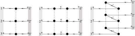
Figure 10: Time ordered graphs of an instantaneous three-body interaction which contribute to the three-quark propagation in the Salpeter equation. The instantaneous three-body kernel is represented by the dashed line.

In the language of time-ordered perturbation theory this means that the instantaneity of the kernel prevents the inclusion of single and double Z-graphs which correspond to the mixed components $\sim\Lambda^{++-},\;\Lambda^{--+},\ldots$, etc. of the interaction kernel. However, compared to a nonrelativistic ansatz, where all three quarks propagate forward in time (corresponding here to the components $\sim\Lambda^{+++}$), the Salpeter equation takes into account also those diagrams, where all three quarks propagate backwards in time (triple Z-graphs corresponding to the components $\sim\Lambda^{---}$ and their coupling to components $\sim\Lambda^{+++}$ via $\overline{\Lambda}^{---}\;V^{(3)}\;\Lambda^{+++}$), as shown in fig. 10. We want to remark here that the appearance of these negative energy components in the Salpeter equation is connected with the particle-antiparticle symmetry due to the ${\cal CPT}$ invariance of the underlying relativistic field theoretical framework. We will come back to this characteristic feature of the Salpeter equation and discuss it in some more detail in sect. 5.2 after we have taken also the two-particle interactions into account. The importance of the negative energy contributions depends on the energy denominators $M\mp(\omega_{1}+\omega_{2}+\omega_{3}-{\rm i}\epsilon)$ of the positive and negative energy components in (95) as can be illustrated by the following two extreme cases:

• For small binding energies, i.e. $M\approx m_{1}+m_{2}+m_{3}$ and $|{\bf p_{i}}|/m_{i}\ll 1$ one has

  $$\frac{1}{M+\omega_{1}+\omega_{2}+\omega_{3}}\ll\frac{1}{M-\omega_{1}-\omega_{2}-\omega_{3}}$$ (102)

  such that the negative energy component in (95) becomes negligible compared to the positive component and one is led to the so-called reduced Salpeter equation.

• For deeply bound states, i.e. $M\ll m_{1}+m_{2}+m_{3}$, both components are of equal order of magnitude:

  $$\frac{1}{M+\omega_{1}+\omega_{2}+\omega_{3}}\approx\frac{1}{M-\omega_{1}-\omega_{2}-\omega_{3}}$$ (103)

In our case of baryons as a bound three-quark system we should definitely be rather far away from the limit of deeply bounds states. Nevertheless the negative energy term of the Salpeter amplitude might contribute to a certain amount.

4.3.2 Hamiltonian formulation of the Salpeter equation

The special projector structure in connection with the particular energy denominators $M\mp(\omega_{1}+\omega_{2}+\omega_{3}-{\rm i}\epsilon)$ allows for the formulation of the Salpeter equation in Hamiltonian form, i.e. as an eigenvalue problem

$${\cal H}\;\Phi_{M}\;\;=\;\;M\;\Phi_{M}\quad\quad\textrm{with}\quad\Lambda\Phi_{M}=\Phi_{M}.$$ (104)

Here we define the Salpeter Hamiltonian ${\cal H}$ by

$$\left[{\cal H}\Phi_{M}\right]({\bf p_{\xi}},{\bf p_{\eta}}) = {\cal H}_{0}({\bf p_{\xi}},{\bf p_{\eta}})\;\Phi_{M}({\bf p_{\xi}},{\bf p_{\eta}})$$

$$+ \left[\Lambda_{1}^{+}({\bf p_{1}})\otimes\Lambda_{2}^{+}({\bf p_{2}})\otimes\Lambda_{3}^{+}({\bf p_{3}})+\Lambda_{1}^{-}({\bf p_{1}})\otimes\Lambda_{2}^{-}({\bf p_{2}})\otimes\Lambda_{3}^{-}({\bf p_{3}})\right]{}$$

$$\times\;\;\gamma^{0}\otimes\gamma^{0}\otimes\gamma^{0}\;\int\frac{\textrm{d}^{3}p_{\xi}^{\prime}}{(2\pi)^{3}}\;\frac{\textrm{d}^{3}p_{\eta}^{\prime}}{(2\pi)^{3}}\;V^{(3)}({\bf p_{\xi}},{\bf p_{\eta}};\;{\bf p_{\xi}^{\prime}},{\bf p_{\eta}^{\prime}})\;\Phi_{M}({\bf p_{\xi}^{\prime}},{\bf p_{\eta}^{\prime}})$$

where the free three-fermion Hamiltonian

$${\cal H}_{0}({\bf p_{\xi}},{\bf p_{\eta}})\;:=\;H_{1}({\bf p_{1}})\otimes{\rm 1\kern-3.00003ptI}\otimes{\rm 1\kern-3.00003ptI}\;\;+\;\;{\rm 1\kern-3.00003ptI}\otimes H_{2}({\bf p_{2}})\otimes{\rm 1\kern-3.00003ptI}\;\;+\;\;{\rm 1\kern-3.00003ptI}\otimes{\rm 1\kern-3.00003ptI}\otimes H_{3}({\bf p_{3}})$$ (106)

represents the relativistic kinetic energy operator.

Of course, a similar representation of the adjoint Salpeter equation, which determines the adjoint amplitude $\overline{\Phi}_{M}$, can also be found. Note however, that both equations are not independent, but even are equivalent, since there is a general interconnection between the Salpeter amplitude $\Phi_{M}$ and its adjoint $\overline{\Phi}_{M}$, which in momentum space reads:

$$\overline{\Phi}_{M}({\bf p_{\xi}},{\bf p_{\eta}})=-\Phi_{M}^{\dagger}({\bf p_{\xi}},{\bf p_{\eta}})\;\gamma^{0}\otimes\gamma^{0}\otimes\gamma^{0}.$$ (107)

To be consistent, one has to require: If $\Phi_{M}$ is a solution of the Salpeter equation (104), then $\overline{\Phi}_{M}$, as defined by relation (107), has to be a solution of the corresponding adjoint Salpeter equation (and vice versa). Using ${\cal H}_{0}^{\dagger}={\cal H}_{0}$ and $\Lambda_{i}^{\dagger}=\Lambda_{i}$, one easily shows that this equivalence of the Salpeter equation (104) and its adjoint implies the following condition for the interaction kernel $V^{(3)}$ in the CMS:

$$V^{(3)}({\bf p_{\xi}},{\bf p_{\eta}};\;{\bf p_{\xi}^{\prime}},{\bf p_{\eta}^{\prime}})\stackrel{{\scriptstyle!}}{{=}}\gamma^{0}\otimes\gamma^{0}\otimes\gamma^{0}\;\left[{V^{(3)}}({\bf p_{\xi}^{\prime}},{\bf p_{\eta}^{\prime}};\;{\bf p_{\xi}},{\bf p_{\eta}})\right]^{\dagger}\;\gamma^{0}\otimes\gamma^{0}\otimes\gamma^{0}$$ (108)

4.3.3 Normalization of Salpeter amplitudes – Scalar product

The normalization condition (63) of the Bethe-Salpeter amplitudes, which reads in the center-of-mass frame with $\bar{P}=(M,{\bf 0})\equiv M$

$$-{\rm i}\;\overline{\chi}_{M}\;\left[\frac{\partial}{\partial P^{0}}\left({G_{0}}_{P}^{-1}+{\rm i}V^{(3)}\right)\right]_{P^{0}=M}\chi_{M}=2M,$$ (109)

induces a normalization condition of the corresponding Salpeter amplitudes $\Phi_{M}$. The instantaneous three-body kernel $V^{(3)}$ has no explicit energy dependence and thus gives no contribution to the norm. Using the representation $\chi_{M}={G_{0}}_{M}\;\Gamma_{M}$ and $\overline{\chi}_{M}=\overline{\Gamma}_{M}\;{G_{0}}_{M}$ of the Bethe-Salpeter amplitudes, where the vertex functions $\Gamma_{M}$ and $\overline{\Gamma}_{M}$ defined in (85) do not depend on the relative energies $p_{\xi}^{0}$, $p_{\eta}^{0}$, eq. (109) becomes

$$2M=-{\rm i}\;\overline{\Gamma}_{M}\;{G_{0}}_{M}\bigg{[}\frac{\partial}{\partial M}\;{G_{0}}_{M}^{-1}\bigg{]}{G_{0}}_{M}\;\Gamma_{M}=\overline{\Gamma}_{M}\left\langle-{\rm i}\;{G_{0}}_{M}\bigg{[}\frac{\partial}{\partial M}\;{G_{0}}_{M}^{-1}\bigg{]}{G_{0}}_{M}\right\rangle\Gamma_{M}.$$ (110)

Here the angled brackets $\langle\ldots\rangle$ indicate the internal integration over $p_{\xi}^{0}$ and $p_{\eta}^{0}$ which is used to reduce the enclosed operator according to eq. (89). With ${G_{0}}_{M}\;(\partial/\partial M\;{G_{0}}_{M}^{-1})\;{G_{0}}_{M}\;=-\partial/\partial M\;{G_{0}}_{M}$ this reduced operator may be rewritten as the derivative of the Salpeter propagator (94) and we obtain

$$\left\langle-{\rm i}\;{G_{0}}_{M}\bigg{[}\frac{\partial}{\partial M}\;{G_{0}}_{M}^{-1}\bigg{]}\;{G_{0}}_{M}\;\right\rangle={\rm i}\frac{\partial}{\partial M}\;\langle{G_{0}}_{M}\rangle=-\langle{G_{0}}_{M}\rangle\;\gamma^{0}\otimes\gamma^{0}\otimes\gamma^{0}\;\langle{G_{0}}_{M}\rangle.$$ (111)

Substitution into eq. (110) and replacing the vertex functions according to the relations $\langle{G_{0}}_{M}\rangle\;\Gamma_{M}=\Phi_{M}$ and $\overline{\Gamma}_{M}\;\langle{G_{0}}_{M}\rangle=\overline{\Phi}_{M}=-\Phi_{M}^{\dagger}\;\gamma^{0}\otimes\gamma^{0}\otimes\gamma^{0}$ then yields the following normalization condition of the Salpeter amplitudes $\Phi_{M}$:

$$\Phi_{M}^{\dagger}\;\Phi_{M}=\int\frac{\textrm{d}^{3}p_{\xi}}{(2\pi)^{3}}\;\frac{\textrm{d}^{3}p_{\eta}}{(2\pi)^{3}}\;\sum_{a_{1},a_{2},a_{3}}\Phi_{M\;a_{1}a_{2}a_{3}}^{*}({\bf p_{\xi}},{\bf p_{\eta}})\;\Phi_{M\;a_{1}a_{2}a_{3}}({\bf p_{\xi}},{\bf p_{\eta}})=2M.$$ (112)

Thus, the solutions $\Phi_{M}$ of the Salpeter equation have to be normalized according to the usual ${\cal L}^{2}$-norm just like the solutions of the ordinary nonrelativistic Schrödinger equation. This norm induces a positive definite scalar product for arbitrary amplitudes $\Phi_{1}$ and $\Phi_{2}$ that are restricted to positive and negative energy components, i.e. $\Phi_{i}=\Lambda\Phi_{i}$:

$$\langle\Phi_{1}|\Phi_{2}\rangle := \int\frac{\textrm{d}^{3}p_{\xi}}{(2\pi)^{3}}\;\frac{\textrm{d}^{3}p_{\eta}}{(2\pi)^{3}}\;\sum_{a_{1},a_{2},a_{3}}\Phi_{1\;a_{1}a_{2}a_{3}}^{*}({\bf p_{\xi}},{\bf p_{\eta}})\;\Phi_{2\;a_{1}a_{2}a_{3}}({\bf p_{\xi}},{\bf p_{\eta}}).$$ (113)

Hence, the normalization condition (112) for solutions $\Phi_{M}$ of the Salpeter equation is then given as

$$\langle\Phi_{M}|\Phi_{M}\rangle=2M.$$ (114)

We want to remark here that a similar treatment of the fermion-antifermion (or the two-fermion) system does not lead to a positive definite scalar product, owing to a relative sign between the positive and negative energy contributions, see ReMu94 .

Note that the Salpeter Hamiltonian ${\cal H}$ is hermitean with respect to the scalar product (113), i.e.

$$\langle\Phi_{1}|{\cal H}\;\Phi_{2}\rangle=\langle{\cal H}\;\Phi_{1}|\Phi_{2}\rangle$$ (115)

which is a direct consequence of the condition (108) on $V^{(3)}$ resulting from the interconnection (107) between $\Phi_{M}$ and $\overline{\Phi}_{M}$. This guarantees, as in the case of the ordinary Schrödinger equation, two important consequences, namely:

• The eigenvalues $M$ of ${\cal H}$, i.e. the three-fermion bound-state masses are real, i.e. $M^{*}=M$.

• Salpeter amplitudes $\Phi_{M_{1}}$ and $\Phi_{M_{2}}$ belonging to different eigenvalues $M_{1}\not=M_{2}$ are mutually orthogonal, i.e. $\langle\Phi_{M_{1}}|\Phi_{M_{2}}\rangle=0$.

4.4 The reduction with genuine two-particle kernels

Now let us come back to the general case we are in fact interested in, where in addition to the instantaneous three-body kernel $V^{(3)}$, the dynamics of the quarks is also determined by the unconnected instantaneously approximated two body-terms given by (68) and (76). Referring again to the formal covariance of the instantaneous approximation as before, we choose for these considerations the three-body rest-frame with $\bar{P}=(M,{\bf 0})\equiv M$. The Bethe-Salpeter equation and its adjoint then read

$$\chi_{M} = -\textrm{i}\;{G_{0}}_{M}\;V^{(3)}\;\chi_{M}-\textrm{i}\;{G_{0}}_{M}\;\overline{K}^{(2)}_{M}\;\chi_{M},$$ (116)

$$\overline{\chi}_{M} = -\textrm{i}\;\overline{\chi}_{M}\;V^{(3)}\;{G_{0}}_{M}-\textrm{i}\;\overline{\chi}_{M}\;\overline{K}^{(2)}_{M}\;{G_{0}}_{M},$$ (117)

and now the difficulty stems from the circumstance that due to the second term on the right hand side of (116), which contains $K^{(2)}_{M}$, the relative energy dependence in the Bethe-Salpeter equation can no longer be separated and thus, from the outset, the reduction cannot be performed. Nevertheless, we still can take advantage of the fact that the $p_{\xi}^{0}$, $p_{\eta}^{0}$ dependence at least is cut by the first term, due to the instantaneity of $V^{(3)}$. Recasting the Bethe-Salpeter equation into a more convenient form, this feature will in fact provide a possibility to perform a reduction, as we will see in the following discussion. But let us emphasize that the way of how to perform the reduction and consequently the final form of the Salpeter equation is not unique, although the various resulting reduced equations are formally equivalent. However, in practice, even the reduced equations are not solvable in general so that further approximations are indispensable and thus the different reduced equations become practically non-equivalent. Therefore, the reduced equation in its full exact form should, right from start, have an expedient canonical structure allowing further approximations to be made in a systematical way. Referring to this we will orientate our considerations according to the instructive canonical form of the Salpeter equation as given in the previously discussed case of vanishing two-body kernels by eqs. (104) and (4.3.2). Before we present this specific method for the reduction of the Bethe-Salpeter equation (116) and its adjoint (117) in practice, let us generally discuss in a first attempt,

• how in principle it becomes possible to reduce the eight-dimensional three-fermion Bethe-Salpeter equation to an equivalent six-dimensional Salpeter equation, provided that the full interaction kernel $K_{P}$ contains at least one connected instantaneous part, as given in our case by the instantaneous three-body kernel,

• what changes at all in the structure and the properties of the Salpeter equation and thus of the Salpeter amplitudes $\Phi_{M}$ in comparison to the case discussed previously, where the dynamics was given by an instantaneous three-body part alone.

4.4.1 A first attempt – concepts, ideas and problems

In a first attempt we now want to sketch a procedure showing that a reduction of the Bethe-Salpeter equation (116) can indeed be achieved, utilizing that $V^{(3)}$ cuts the relative energy dependence in one term of the Bethe-Salpeter equation. The crucial idea and concept of this procedure is to get rid of the problematical second term $-\textrm{i}\;{G_{0}}_{M}\;\overline{K}^{(2)}_{M}\;\chi_{M}$ appearing on the right hand side of eq. (116), where the unconnected two-body term $\overline{K}^{(2)}_{M}$ acts on the Bethe-Salpeter amplitude $\chi_{M}$ directly. This can be reached by recasting the Bethe-Salpeter equation (116) in the following manner. First we separate the terms of the Bethe-Salpeter equation into $p_{\xi}^{0}$, $p_{\eta}^{0}$ dependent and independent parts, as follows:

$$\left[{G^{-1}_{0}}_{M}\;+\textrm{i}\;\overline{K}^{(2)}_{M}\right]\;\chi_{M}=-\textrm{i}\;V^{(3)}\;\chi_{M}$$ (118)

Remember that $-\textrm{i}\;V^{(3)}\;\chi_{M}$ on the right hand side indeed has no relative energy dependence due to eq. (85). Now let us introduce the resolvent $\overline{\cal G}_{M}^{(2)}$ of the operator $[{G^{-1}_{0}}_{M}\;+\textrm{i}\;\overline{K}^{(2)}_{M}]$ appearing on the left hand side of the eqs. (118), i.e.

$$\overline{\cal G}_{M}^{(2)}\;\left[{G^{-1}_{0}}_{M}\;+\textrm{i}\;\overline{K}^{(2)}_{M}\right]=\left[{G^{-1}_{0}}_{M}\;+\textrm{i}\;\overline{K}^{(2)}_{M}\right]\;\overline{\cal G}_{M}^{(2)}={\rm 1\kern-3.00003ptI}.$$ (119)

This Green’s function $\overline{\cal G}_{M}^{(2)}$ is the solution of the inhomogeneous eight-dimensional integral equation

$$\overline{\cal G}_{M}^{(2)} = {G_{0}}_{M}-\textrm{i}\;{G_{0}}_{M}\;\overline{K}^{(2)}_{M}\;\overline{\cal G}_{M}^{(2)}$$ (120)

and thus describes, apart from the free propagation ${G_{0}}_{M}$, also the propagation of the three quarks via the unconnected two-particle interactions alone. Multiplying eq. (118) by this resolvent $\overline{\cal G}_{M}^{(2)}$ we obtain the Bethe-Salpeter equation in a form similar to (77), i.e. the case where we neglected the two-particle forces, but with ${G_{0}}_{M}$ now replaced by $\overline{\cal G}_{M}^{(2)}$ which additionally collects all remaining retardation effects concerning the unconnected two-quark interactions within the baryon:

$$\chi_{M}=-{\rm i}\;\overline{\cal G}_{M}^{(2)}\;V^{(3)}\;\chi_{M}.$$ (121)

This form enables us again to exploit the crucial property of the instantaneous kernel $V^{(3)}$ to separate the dependence on the relative energy variables ${p_{\xi}}^{0}$ and ${p_{\eta}}^{0}$. Consequently we can proceed in the same way to reduce the Bethe-Salpeter equations (121) as we did when reducing eq. (77) in the case of vanishing two-quark kernels. According to eq. (79) the eight-dimensional integral operation $V^{(3)}$ on $\chi_{M}$ on the right hand side of eq. (121) can be reduced to a six-dimensional operation on the Salpeter amplitude $\Phi_{M}$,

$$\left[V^{(3)}\;\chi_{M}\right]({p_{\xi}},{p_{\eta}})=\left[V^{(3)}\;\Phi_{M}\right]({\bf p_{\xi}},{\bf p_{\eta}}).$$ (122)

This (in principle) provides us again the possibility to reconstruct the full eight-dimensional Bethe-Salpeter amplitude $\chi_{M}$ from the Salpeter amplitude $\Phi_{M}$ according to

$$\chi_{M}=-{\rm i}\;\overline{\cal G}_{M}^{(2)}\;V^{(3)}\;\Phi_{M}$$ (123)

and shows that the analytical $p_{\xi}^{0}$, $p_{\eta}^{0}$ dependence of the Bethe-Salpeter amplitude is completely determined by the analytical structure of $\overline{\cal G}_{M}^{(2)}$ in these variables. Thus, performing the $p_{\xi}^{0},p_{\eta}^{0}$ integration on both sides of eq. (123), the Bethe-Salpeter amplitude $\chi_{M}$ on the left reduces to the Salpeter amplitude $\Phi_{M}$ and on the right hand side only $\overline{\cal G}_{M}^{(2)}$ is affected by this integration and reduces to $\langle\overline{\cal G}_{M}^{(2)}\rangle$. Consequently, we finally end up with the reduced equation which determines the Salpeter amplitude $\Phi_{M}$, i.e.

$$\Phi_{M}\;=\;-{\rm i}\;\left\langle\overline{\cal G}_{M}^{(2)}\right\rangle\;V^{(3)}\;\Phi_{M}.$$ (124)

All the difficulties, arising from retardation effects due to the unconnected two-body terms, are now transferred to the reduction $\langle\overline{\cal G}_{M}^{(2)}\rangle$ of $\overline{\cal G}_{M}^{(2)}$. Corresponding to the inhomogeneous integral equation (120) this reduction of the Green’s function is determined by

$$\left\langle\overline{\cal G}_{M}^{(2)}\right\rangle = \left\langle{G_{0}}_{M}\right\rangle-\textrm{i}\;\left\langle{G_{0}}_{M}\;\overline{K}^{(2)}_{M}\;\overline{\cal G}_{M}^{(2)}\right\rangle{}$$ (125)

$$= \left\langle{G_{0}}_{M}\right\rangle\;+\;\left\langle{G_{0}}_{M}\left[-\textrm{i}\;\overline{K}^{(2)}_{M}\right]{G_{0}}_{M}\right\rangle\;+\;\left\langle{G_{0}}_{M}\left[-\textrm{i}\;\overline{K}^{(2)}_{M}\right]{G_{0}}_{M}\left[-\textrm{i}\;\overline{K}^{(2)}_{M}\right]{G_{0}}_{M}\right\rangle{}$$

$$\phantom{\langle{G_{0}}_{M}\rangle}\;+\;\ldots\;.$$

Thus, we have shown that, even with unconnected two-particle kernels, it is in principle possible to reduce the eight-dimensional three-fermion Bethe-Salpeter equation to a six-dimensional Salpeter equation, provided we choose at least one part of the full interaction kernel to be instantaneous. Due to the interconnection (123) of the full eight-dimensional Bethe-Salpeter amplitude $\chi_{M}$ and its six-dimensional reduction, i.e. the Salpeter amplitude $\Phi_{M}$, the Salpeter equation is equivalent to the full Bethe-Salpeter equation since eq. (123) provides in principle an equally exact reconstruction of the Bethe-Salpeter amplitude. Unfortunately, the analytical structure of the Green’s function $\overline{\cal G}_{M}^{(2)}$ in the complex planes of the relative energy variables $p_{\xi}^{0}$ and $p_{\eta}^{0}$ is rather complicated, so that in practice neither its reduction $\langle\overline{\cal G}_{M}^{(2)}\rangle$ required for solving the Salpeter equation (124), nor $\overline{\cal G}_{M}^{(2)}$ itself, required for the reconstruction (123) of the Bethe-Salpeter amplitude, is manageable in its full, exact form. The determination of $\langle\overline{\cal G}_{M}^{(2)}\rangle$ for example requires in principle the calculation of an infinite number of reduced diagrams due to the Neumann series of $\overline{\cal G}_{M}^{(2)}$, see eq. (125). We do not want to bother about that complexity at the moment and first consider $\langle\overline{\cal G}_{M}^{(2)}\rangle$ in eq. (124) only up to the Born term,

$$\Phi_{M}\;=\;\left[-\textrm{i}\;\left\langle{G_{0}}_{M}\right\rangle\;-\;\left\langle{G_{0}}_{M}\;\overline{K}^{(2)}_{M}\;{G_{0}}_{M}\right\rangle\;+\;\ldots\right]\;V^{(3)}\;\Phi_{M}$$ (126)

in order to inspect what changes basically in the structure of the Salpeter equation and the corresponding Salpeter amplitudes. A tedious but straightforward calculation, using the residue theorem for performing the relative energy integration, yields the following contributions to the reduced Born term:

$$-\left\langle{G_{0}}_{M}\;\overline{K}^{(2)}_{M}\;{G_{0}}_{M}\right\rangle({\bf p_{\xi}},{\bf p_{\eta}};\;{\bf p_{\xi}^{\prime}},{\bf p_{\eta}^{\prime}})\;\;=\;\;$$

$$\Bigg{\{} + \frac{\Lambda^{+}_{1}\otimes\Lambda^{+}_{2}\otimes\Lambda^{+}_{3}\;\gamma^{0}\otimes\gamma^{0}\otimes\gamma^{0}}{M-\omega_{1}-\omega_{2}-\omega_{3}+{\rm i}\;\epsilon}\;\left[V^{(2)}({\bf p_{\xi}},{\bf p_{\xi}^{\prime}})\otimes\gamma^{0}\right]\;\frac{{\Lambda^{+}_{1}}^{\prime}\otimes{\Lambda^{+}_{2}}^{\prime}\otimes{\Lambda^{+}_{3}}^{\prime}\;\gamma^{0}\otimes\gamma^{0}\otimes\gamma^{0}}{M-\omega_{1}^{\prime}-\omega_{2}^{\prime}-\omega_{3}^{\prime}+{\rm i}\;\epsilon}\;{\bf(a)}{}$$ (129)

$$- \frac{\Lambda^{-}_{1}\otimes\Lambda^{-}_{2}\otimes\Lambda^{-}_{3}\;\gamma^{0}\otimes\gamma^{0}\otimes\gamma^{0}}{M+\omega_{1}+\omega_{2}+\omega_{3}-{\rm i}\;\epsilon}\;\left[V^{(2)}({\bf p_{\xi}},{\bf p_{\xi}^{\prime}})\otimes\gamma^{0}\right]\;\frac{{\Lambda^{-}_{1}}^{\prime}\otimes{\Lambda^{-}_{2}}^{\prime}\otimes{\Lambda^{-}_{3}}^{\prime}\;\gamma^{0}\otimes\gamma^{0}\otimes\gamma^{0}}{M+\omega_{1}^{\prime}+\omega_{2}^{\prime}+\omega_{3}^{\prime}-{\rm i}\;\epsilon}\;{\bf(b)}{}$$

$$- \frac{\Lambda^{+}_{1}\otimes\Lambda^{+}_{2}\otimes\Lambda^{+}_{3}\;\gamma^{0}\otimes\gamma^{0}\otimes\gamma^{0}}{M-\omega_{1}-\omega_{2}-\omega_{3}+{\rm i}\;\epsilon}\;\left[V^{(2)}({\bf p_{\xi}},{\bf p_{\xi}^{\prime}})\otimes\gamma^{0}\right]\;\frac{{\Lambda^{-}_{1}}^{\prime}\otimes{\Lambda^{-}_{2}}^{\prime}\otimes{\Lambda^{+}_{3}}^{\prime}\;\gamma^{0}\otimes\gamma^{0}\otimes\gamma^{0}}{\omega_{1}+\omega_{2}+\omega_{1}^{\prime}+\omega_{2}^{\prime}}\;{\bf(c)}{}$$

$$- \frac{\Lambda^{-}_{1}\otimes\Lambda^{-}_{2}\otimes\Lambda^{-}_{3}\;\gamma^{0}\otimes\gamma^{0}\otimes\gamma^{0}}{M+\omega_{1}+\omega_{2}+\omega_{3}-{\rm i}\;\epsilon}\;\left[V^{(2)}({\bf p_{\xi}},{\bf p_{\xi}^{\prime}})\otimes\gamma^{0}\right]\;\frac{{\Lambda^{+}_{1}}^{\prime}\otimes{\Lambda^{+}_{2}}^{\prime}\otimes{\Lambda^{-}_{3}}^{\prime}\;\gamma^{0}\otimes\gamma^{0}\otimes\gamma^{0}}{\omega_{1}+\omega_{2}+\omega_{1}^{\prime}+\omega_{2}^{\prime}}\;{\bf(d)}{}$$

$$- \frac{\Lambda^{-}_{1}\otimes\Lambda^{-}_{2}\otimes\Lambda^{+}_{3}\;\gamma^{0}\otimes\gamma^{0}\otimes\gamma^{0}}{\omega_{1}+\omega_{2}+\omega_{1}^{\prime}+\omega_{2}^{\prime}}\;\left[V^{(2)}({\bf p_{\xi}},{\bf p_{\xi}^{\prime}})\otimes\gamma^{0}\right]\;\frac{{\Lambda^{+}_{1}}^{\prime}\otimes{\Lambda^{+}_{2}}^{\prime}\otimes{\Lambda^{+}_{3}}^{\prime}\;\gamma^{0}\otimes\gamma^{0}\otimes\gamma^{0}}{M-\omega_{1}^{\prime}-\omega_{2}^{\prime}-\omega_{3}^{\prime}+{\rm i}\;\epsilon}\;{\bf(e)}{}$$

$$- \frac{\Lambda^{+}_{1}\otimes\Lambda^{+}_{2}\otimes\Lambda^{-}_{3}\;\gamma^{0}\otimes\gamma^{0}\otimes\gamma^{0}}{\omega_{1}+\omega_{2}+\omega_{1}^{\prime}+\omega_{2}^{\prime}}\;\left[V^{(2)}({\bf p_{\xi}},{\bf p_{\xi}^{\prime}})\otimes\gamma^{0}\right]\;\frac{{\Lambda^{-}_{1}}^{\prime}\otimes{\Lambda^{-}_{2}}^{\prime}\otimes{\Lambda^{-}_{3}}^{\prime}\;\gamma^{0}\otimes\gamma^{0}\otimes\gamma^{0}}{M+\omega_{1}^{\prime}+\omega_{2}^{\prime}+\omega_{3}^{\prime}-{\rm i}\;\epsilon}\;{\bf(f)}{}$$

$$\Bigg{\}}\;(2\pi)^{3}\;\delta^{(3)}({\bf p_{\eta}}-{\bf p_{\eta}^{\prime}})\;+\;\begin{array}[]{l}\textrm{cyclic. perm. of $(12)\;3$ corresponding to the}\\ \textrm{interacting quark pairs (23) and (31)}\end{array}$$

For the sake of clarity we suppressed partially the explicit coordinate dependences by using the more compact notation $\Lambda^{\pm}_{i}\equiv\Lambda^{\pm}_{i}({\bf p_{i}})$, $\omega_{i}\equiv\omega_{i}({\bf p_{i}})$ and ${\Lambda^{\pm}_{i}}^{\prime}\equiv\Lambda^{\pm}_{i}({\bf p_{i}^{\prime}})$, $\omega_{i}^{\prime}\equiv\omega_{i}({\bf p_{i}^{\prime}})$. The time-ordered Feynman graphs corresponding to the six different terms in eq. (129) are shown in fig. 11.

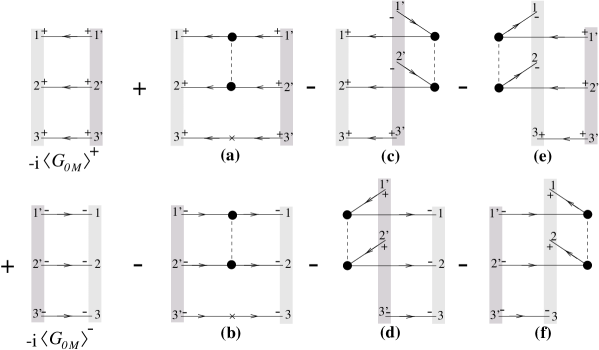
Figure 11: Time ordered graphs of the reduced Green’s function $\langle\overline{\cal G}_{M}^{(2)}\rangle$ up to the Born term (only the interactions in the quark pair (12) are shown.) The instantaneous two-body interaction between two quarks is represented by the vertical dashed lines and dots on the affected quark lines. The Born graphs correspond to the expressions of eq. (129).

The first two terms (a) and (b) have the same projector structure and corresponding energy denominators as the Salpeter propagator $\langle{G_{0}}_{M}\rangle$ and thus are of a similar form as the reduction of a genuine instantaneous three-body interaction diagram. The decisive difference to the previously discussed case is due to the occurrence of the mixed energy components $(++-)$, $(--+)$, etc. in the remaining four terms (c) - (f), which result from retardation effects of the unconnected two-particle interactions. In other words: The propagator $\langle\overline{\cal G}_{M}^{(2)}\rangle$ which has been substituted for $\langle{G_{0}}_{M}\rangle$ (compared to the case of neglected two-body kernels) does not exhibit the particular projection properties of $\langle{G_{0}}_{M}\rangle$, i.e. the restriction to purely positive and purely negative energy components only. This implies (compare the discussion in subsect. 4.3.1):

• The Salpeter amplitudes $\Phi_{M}$ are no longer eigenstates of the Salpeter projector $\Lambda$, but also possess mixed energy components according to the terms (e) and (f) in (129).

• In connection with the unconnected, retarded two-particle kernels, also the ’residual’ part $V_{\rm R}^{(3)}=V^{(3)}-V_{\Lambda}^{(3)}$ of the instantaneous three-body kernel $V^{(3)}$, that couples to the mixed components, now contributes to the three-fermion bound state and therefore to the spectroscopic results.

Note however, that (assuming weakly bound states) the important dominant terms of this Born contribution are given by the purely positive and negative contributions (a) and (b) due to their particular structure of the energy denominators:

• In the case ${\bf M>0}$ the terms (c) and (e) are suppressed with respect to the dominant term (a), since $(M-\omega_{1}-\omega_{2}-\omega_{3})^{-1}\gg(\omega_{1}+\omega_{2}+\omega_{1}^{\prime}+\omega_{2}^{\prime})^{-1}$. All other contributions have denominators $(M+\omega_{1}+\omega_{2}+\omega_{3})$ and thus are anyhow suppressed.

• In the case ${\bf M<0}$ the dominant term is (b), whereas (d) and (f) are suppressed against (b), since $(M+\omega_{1}+\omega_{2}+\omega_{3})^{-1}\gg(\omega_{1}+\omega_{2}+\omega_{1}^{\prime}+\omega_{2}^{\prime})^{-1}$ All other contributions have denominators $(M-\omega_{1}-\omega_{2}-\omega_{3})$ and hence are anyway negligible.

The more complex structure of the Salpeter equation (124) restricts its applicability to explicit three-body bound-state calculations: Due to the explicit appearance of the additional mixed energy components the formulation as an eigenvalue problem in Hamiltonian form such as in the case of a pure instantaneous three-body kernel is no longer possible. Moreover further approximations of the reduced Green’s function $\langle\overline{\cal G}_{M}^{(2)}\rangle$ are indispensable, which gives rise to the question of how to approximate $\langle\overline{\cal G}_{M}^{(2)}\rangle$ systematically. One would expect that a perturbative approximation of $\langle\overline{\cal G}_{M}^{(2)}\rangle$ simply by cutting the Neumann series of $\overline{\cal G}_{M}^{(2)}$ at finite order (e.g. in the so far considered Born approximation), would not be sufficient to describe accurately the effects of the two-particle interaction within a three-body bound state, as e.g. two particle correlations. In order to take non-perturbatively at least an infinite subset of diagrams of $\langle\overline{\cal G}_{M}^{(2)}\rangle$ into account, one could follow an idea of Phillips and Wallace PhWa96 ; PhWa98 ; LaAf97 , who investigated the three-dimensional reduction of the two-fermion Bethe-Salpeter equation with general four-dimensional (i.e. non-instantaneous) interaction kernels. Their method provides a generalization of a former formalism of Klein Kl53 ; Kl54 using the quasi-potential approach of Logunov and Tavkhelidze LoTa63 and has a close connection to standard time-ordered perturbation theory. Applying their idea to our three-body case, their method essentially consists in a systematical prescription to determine order-by-order (in the coupling of $\overline{K}^{(2)}_{M}$) an instantaneous three-particle irreducible kernel $\overline{K}^{(2)}_{M\;{\rm inst}}$, where irreducibility is now defined with respect to the Salpeter propagator $\langle{G_{0}}_{M}\rangle$, such that

$$\langle\overline{\cal G}_{M}^{(2)}\rangle=\langle{G_{0}}_{M}\rangle-{\rm i}\;\langle{G_{0}}_{M}\rangle\;\overline{K}^{(2)}_{M\;{\rm inst}}\langle\overline{\cal G}_{M}^{(2)}\rangle.$$ (130)

This would allow for a formulation of the Salpeter equation (124) in a form that is the same as in the previously discussed case of vanishing two body interactions, i.e.

$$\Phi_{M}=-{\rm i}\;\langle{G_{0}}_{M}\rangle\left[\overline{K}^{(2)}_{M\;{\rm inst}}+V^{(3)}\right]\;\Phi_{M}.$$ (131)

However, the method of PhWa96 ; PhWa98 has an inconsistency pointed out by the authors themselves: Obviously, eqs. (130) and (131) are in clear contradiction to the occurrence of mixed energy components discussed above: due to the projector property of $\langle{G_{0}}_{M}\rangle$, eq. (130) would restrict $\langle\overline{\cal G}_{M}^{(2)}\rangle$ and consequently $\Phi_{M}$ to purely positive and negative components only. In the next subsection we will therefore improve our reduction procedure such that this method nevertheless becomes applicable without revealing such inconsistencies.

4.4.2 Reduction to a Salpeter equation in Hamiltonian form

In this subsection we present a systematical reduction procedure, which avoids the difficulties and inconsistencies of the foregoing first attempt and allows for a formulation of the Salpeter equation with a structure quite similar to that of sect. 4.3, where the dynamics was given by a connected instantaneous three-body interaction alone. Furthermore, this procedure will provide a systematic approximation of the exact reduced equation that is still manageable in practice and appropriate for explicit calculations. Our aim is to get a reduction of the Bethe-Salpeter equation which even in the presence of unconnected two-quark kernels exhibits the same form and properties as the Salpeter equation (87) in the case of vanishing two-body terms. Consequently it then can likewise be formulated as an eigenvalue problem (or at least as a generalized eigenvalue problem) in Hamiltonian form as discussed in subsect. 4.3.2. In other words:

• The free three-quark propagation shall be given by the Salpeter propagator $\langle{G_{0}}_{M}\rangle$. Accordingly, we search for an instantaneous three-particle irreducible kernel $V^{\rm eff}_{M}$ (a quasi potential) with irreducibility defined with respect to the propagator $\langle{G_{0}}_{M}\rangle$, which covers all the complexity arising from the unconnected two-particle interactions and adds to the genuine instantaneous three-quark kernel $V^{(3)}$.

• Due to the projector property of the Salpeter propagator

  $$\Lambda\langle{G_{0}}_{M}\rangle=\langle{G_{0}}_{M}\rangle\overline{\Lambda}=\langle{G_{0}}_{M}\rangle$$ (132)

  where $\Lambda$ and $\overline{\Lambda}$ are the Salpeter projectors defined in eq. (96) and (97), the reduced equation then merely involves the purely positive and purely negative energy components. Consequently the reduced amplitudes emerging from the Salpeter equation and its adjoint must be eigenstates of the Salpeter projector $\Lambda$ and $\overline{\Lambda}$, respectively.

• However, as demonstrated in the previous discussion of subsect. 4.4.1, the Salpeter amplitude itself is no longer an eigenstate of the Salpeter projector when two-particle interactions are taken into account. We found that in this case also the mixed energy components occur. Consequently, the reduced amplitude resulting from our desired reduced equation can not be the full Salpeter amplitude $\Phi_{M}$ but only its projected part $\Phi_{M}^{\Lambda}:=\Lambda\Phi_{M}$. To summarize, we are looking for a reduction of the Bethe-Salpeter equation of the form

  $$\Phi_{M}^{\Lambda}=-\textrm{i}\;\langle{G_{0}}_{M}\rangle\;\left[V^{(3)}+V^{\rm eff}_{M}\right]\;\Phi^{\Lambda}_{M}\quad\textrm{with}\quad\Phi_{M}^{\Lambda}:=\Lambda\Phi_{M}.$$ (133)

  Equivalence to the Salpeter equation (124) then requires that all interactions via the mixed components must be effectively taken into account in the quasi-potential $V^{\rm eff}_{M}$ and moreover there must be an interconnection which allows to regain the full Salpeter amplitude $\Phi_{M}$ and finally the full Bethe-Salpeter amplitude $\chi_{M}$ from the projected amplitude $\Phi_{M}^{\Lambda}$.

Now let us become specific and show how such a kind of reduction can indeed be achieved. To this end we split the instantaneous three-body kernel $V^{(3)}$ according to

$$V^{(3)}=V^{(3)}_{\Lambda}+V^{(3)}_{\rm R},$$ (134)

with $V^{(3)}_{\Lambda}$ that part of $V^{(3)}$ which couples exclusively to purely positive and purely negative energy states, i.e.

$$V^{(3)}_{\Lambda}({\bf p_{\xi}},{\bf p_{\eta}};\;{\bf p_{\xi}^{\prime}},{\bf p_{\eta}^{\prime}}) := \overline{\Lambda}({\bf p_{\xi}},{\bf p_{\eta}})\;V^{(3)}({\bf p_{\xi}},{\bf p_{\eta}};\;{\bf p_{\xi}^{\prime}},{\bf p_{\eta}^{\prime}})\;\Lambda(\;{\bf p_{\xi}^{\prime}},{\bf p_{\eta}^{\prime}})$$ (135)

and the residual part $V^{(3)}_{\rm R}:=V^{(3)}-V^{(3)}_{\Lambda}$, which couples also to the mixed energy components and has the property

$$\overline{\Lambda}\;V^{(3)}_{\rm R}\;\Lambda\equiv 0.$$ (136)

Then we have for the Bethe-Salpeter equation and its adjoint:

$$\chi_{M} = -\textrm{i}\;{G_{0}}_{M}\;\left[V^{(3)}_{\Lambda}+V^{(3)}_{\rm R}+\overline{K}^{(2)}_{M}\right]\;\chi_{M},$$ (137)

$$\overline{\chi}_{M} = -\textrm{i}\;\overline{\chi}_{M}\;\left[V^{(3)}_{\Lambda}+V^{(3)}_{\rm R}+\overline{K}^{(2)}_{M}\right]\;{G_{0}}_{M}.$$ (138)

Recall that in the case of vanishing two-particle kernels only the first part $V^{(3)}_{\Lambda}$ contributes to the Salpeter equation, while the residual part $V^{(3)}_{\rm R}$ disappears according to property (136), as discussed in subsect. 4.3.1. But now, in connection with retardation effects of the unconnected two-particle terms, also the residual part $V^{(3)}_{\rm R}$ gives contributions to the reduction of the Bethe-Salpeter equation as has been shown in the previous subsect. 4.4.1. Keeping this in mind we now want to proceed in a way similar to our first attempt in subsect. 4.4.1, where we transfered the effects of the retarded two-particle terms $\overline{K}^{(2)}_{M}$ into the Green’s function $\overline{\cal G}_{M}^{(2)}$. However, our discussion indicates that it is even more convenient to absorb together with $\overline{K}^{(2)}_{M}$ also the instantaneous kernel $V^{(3)}_{\rm R}$ into a Green’s function ${\cal G}_{M}$, since the contributions of $V^{(3)}_{\rm R}$ occur exclusively in connection with $\overline{K}^{(2)}_{M}$. In this way we achieve that really all complications resulting from the unconnected two body-terms are gathered in the resolvent ${\cal G}_{M}$, which now is defined by

$${\cal G}_{M}\;\left[{G^{-1}_{0}}_{M}\;+\textrm{i}\;V^{(3)}_{\rm R}+\textrm{i}\;\overline{K}^{(2)}_{M}\right]=\left[{G^{-1}_{0}}_{M}\;+\textrm{i}\;V^{(3)}_{\rm R}+\textrm{i}\;\overline{K}^{(2)}_{M}\right]\;{\cal G}_{M}={\rm 1\kern-3.00003ptI}$$ (139)

and thus is the solution of the inhomogeneous integral equations

$${\cal G}_{M}={G_{0}}_{M}-\textrm{i}\;{G_{0}}_{M}\;\left[V^{(3)}_{\rm R}+\overline{K}^{(2)}_{M}\right]\;{\cal G}_{M}={G_{0}}_{M}-\textrm{i}\;{\cal G}_{M}\;\left[V^{(3)}_{\rm R}+\overline{K}^{(2)}_{M}\right]\;{G_{0}}_{M}.$$ (140)

With ${\cal G}_{M}$ the Bethe-Salpeter equation and its adjoint can be rewritten as before in the equivalent form

$$\chi_{M} = -\textrm{i}\;{\cal G}_{M}\;V^{(3)}_{\Lambda}\;\chi_{M},$$ (141)

$$\overline{\chi}_{M} = -\textrm{i}\;\overline{\chi}_{M}\;V^{(3)}_{\Lambda}\;{\cal G}_{M},$$ (142)

which is suited for the six-dimensional reduction, because the new three-body kernel $V^{(3)}_{\Lambda}$ is instantaneous. The reduction is performed as before. Similar to eq. (79) we obtain first

$$\left[V^{(3)}_{\Lambda}\;\chi_{M}\right](p_{\xi},p_{\eta}) = \left[V^{(3)}_{\Lambda}\;\Phi_{M}\right]({\bf p_{\xi}},{\bf p_{\eta}})$$ (143)

$$\left[\overline{\chi}_{M}\;V^{(3)}_{\Lambda}\right](p_{\xi},p_{\eta}) = \left[\overline{\Phi}_{M}\;V^{(3)}_{\Lambda}\right]({\bf p_{\xi}},{\bf p_{\eta}}),$$ (144)

where the Salpeter amplitudes $\Phi_{M}$ and $\overline{\Phi}_{M}$ are the reductions of the corresponding Bethe-Salpeter amplitudes as defined in eqs. (80) and (82). Inserting this back into the Bethe-Salpeter equations we get the prescription how to reconstruct the full eight-dimensional Bethe-Salpeter amplitudes from the Salpeter amplitudes:

$$\chi_{M} = -\textrm{i}\;{\cal G}_{M}\;V^{(3)}_{\Lambda}\;\Phi_{M},$$ (145)

$$\overline{\chi}_{M} = -\textrm{i}\;\overline{\Phi}_{M}\;V^{(3)}_{\Lambda}\;{\cal G}_{M}.$$ (146)

However, with the definition $V^{(3)}_{\Lambda}=\overline{\Lambda}V^{(3)}\Lambda$, we in fact have

$$\chi_{M} = -\textrm{i}\;{\cal G}_{M}\;\overline{\Lambda}V^{(3)}\;\Phi_{M}^{\Lambda}$$ (147)

$$\overline{\chi}_{M} = -\textrm{i}\;\overline{\Phi}_{M}^{\Lambda}\;V^{(3)}\Lambda\;{\cal G}_{M}$$ (148)

showing that for a reconstruction of the full eight-dimensional Bethe-Salpeter amplitudes it indeed suffices to know only the projected components

$$\Phi_{M}^{\Lambda}\left({\bf p_{\xi}},{\bf p_{\eta}}\right) := \Lambda\left({\bf p_{\xi}},{\bf p_{\eta}}\right)\;\Phi_{M}\left({\bf p_{\xi}},{\bf p_{\eta}}\right),$$ (149)

$$\overline{\Phi}_{M}^{\Lambda}\left({\bf p_{\xi}},{\bf p_{\eta}}\right) := \overline{\Phi}_{M}\left({\bf p_{\xi}},{\bf p_{\eta}}\right)\;\overline{\Lambda}\left({\bf p_{\xi}},{\bf p_{\eta}}\right)$$ (150)

of the Salpeter amplitudes. Performing now the integration over ${p_{\xi}}^{0}$ and ${p_{\eta}}^{0}$ on both sides of eqs. (147) and (148), the Bethe-Salpeter amplitudes $\chi_{M}$ and $\overline{\chi}_{M}$ on the left hand side reduce to the Salpeter amplitudes $\Phi_{M}$ and $\overline{\Phi}_{M}$ and on the right hand side we obtain the reduction $\langle{\cal G}_{M}\rangle$ of the resolvent ${\cal G}_{M}$ leading to the interconnection between the full Salpeter amplitudes $\Phi_{M}$ and $\overline{\Phi}_{M}$ and their corresponding projected parts $\Phi_{M}^{\Lambda}$ and $\overline{\Phi}_{M}^{\Lambda}$, respectively, i.e.

$$\Phi_{M} = -\textrm{i}\;\langle{\cal G}_{M}\rangle\;\overline{\Lambda}V^{(3)}\;\Phi^{\Lambda}_{M},$$ (151)

$$\overline{\Phi}_{M} = -\textrm{i}\;\overline{\Phi}_{M}^{\Lambda}\;V^{(3)}\Lambda\;\langle{\cal G}_{M}\rangle.$$ (152)

Here the mixed energy components of the full amplitudes $\Phi_{M}$ and $\overline{\Phi}_{M}$ reenter via the mixed energy components of $\langle{\cal G}_{M}\rangle$. To get the equations for the components $\Phi_{M}^{\Lambda}$ and $\overline{\Phi}_{M}^{\Lambda}$, we finally have to perform the projection on purely positive and purely negative energy components via the Salpeter projectors $\Lambda$ and $\overline{\Lambda}$ on both sides of the eqs. (151) and (152), respectively. We then find

$$\Phi_{M}^{\Lambda} = -\textrm{i}\;\langle{\cal G}_{M}\rangle_{\Lambda}\;V^{(3)}\;\Phi^{\Lambda}_{M},$$ (153)

$$\overline{\Phi}_{M}^{\Lambda} = -\textrm{i}\;\overline{\Phi}_{M}^{\Lambda}\;V^{(3)}\;\langle{\cal G}_{M}\rangle_{\Lambda},$$ (154)

where we introduced the symbol $\langle{\cal G}_{M}\rangle_{\Lambda}$ to denote the corresponding projection on $\langle{\cal G}_{M}\rangle$,

$$\langle{\cal G}_{M}\rangle_{\Lambda} := \Lambda\langle{\cal G}_{M}\rangle\overline{\Lambda},$$ (155)

which cuts off the mixed energy components on both sides of $\langle{\cal G}_{M}\rangle$. Thus, due to the Neumann series of ${\cal G}_{M}$, the reduced propagator $\langle{\cal G}_{M}\rangle_{\Lambda}$ may be represented as power series which starts in lowest order with the free Salpeter propagator $\langle{G_{0}}_{M}\rangle$ and consists of an infinite number of reduced Feynman diagrams, which all are restricted to purely positive and negative energy components, as the Salpeter propagator $\langle{G_{0}}_{M}\rangle$ itself:

$$\langle{\cal G}_{M}\rangle_{\Lambda} = \langle{G_{0}}_{M}\rangle+\;\Lambda\left\langle{G_{0}}_{M}\;(-\textrm{i})\left[V^{(3)}_{\rm R}+\overline{K}^{(2)}_{M}\right]\;{G_{0}}_{M}\right\rangle\overline{\Lambda}$$

$$\;+\;\Lambda\left\langle{G_{0}}_{M}\;(-\textrm{i})\left[V^{(3)}_{\rm R}+\overline{K}^{(2)}_{M}\right]\;{G_{0}}_{M}\;(-\textrm{i})\left[V^{(3)}_{\rm R}+\overline{K}^{(2)}_{M}\right]\;{G_{0}}_{M}\right\rangle\overline{\Lambda}\;+\;\ldots\;.$$

The idea is now to classify the reducible and irreducible diagrams in this infinite reduced series in the same way as done in sect. 2, where the quantum field theoretical six-point Green’s function $G$ was non-perturbatively constructed as a solution of an inhomogeneous eight-dimensional integral equation. But now this classification is done on the reduced level where irreducibility is understood with respect to the ’free’ Salpeter propagator $\langle{G_{0}}_{M}\rangle$. This means that we are looking for an irreducible kernel $V^{\rm eff}_{M}$ such that $\langle{\cal G}_{M}\rangle_{\Lambda}$ is the solution of the following six-dimensional integral equation:

$$\langle{\cal G}_{M}\rangle_{\Lambda}\;\stackrel{{\scriptstyle!}}{{=}}\;\langle{G_{0}}_{M}\rangle-\textrm{i}\;\langle{G_{0}}_{M}\rangle\;V^{\rm eff}_{M}\;\langle{\cal G}_{M}\rangle_{\Lambda}\;=\;\langle{G_{0}}_{M}\rangle-\textrm{i}\;\langle{\cal G}_{M}\rangle_{\Lambda}\;V^{\rm eff}_{M}\;\langle{G_{0}}_{M}\rangle.$$ (157)

Note that in contrast to our first attempt, where this ansatz due to the restrictive action of the Salpeter propagator $\langle{G_{0}}_{M}\rangle$ on purely positive and negative energy components led to inconsistencies, here the ansatz becomes possible now, because $\langle{\cal G}_{M}\rangle_{\Lambda}$ itself and thus all terms of the series (4.4.2) have by construction the same restriction as $\langle{G_{0}}_{M}\rangle$ to these components only. Formally the determination of $V^{\rm eff}_{M}$ corresponds to the inversion of $\langle{\cal G}_{M}\rangle_{\Lambda}$, which due to the projector properties is restricted to the subspace of positive and negative energy components. In particular, this requires the inversion of the Salpeter propagator $\langle{G_{0}}_{M}\rangle$ in this subspace. For this purpose we introduce the operator ${h_{0}}_{M}$ by

$${h_{0}}_{M}({\bf p_{\xi}},{\bf p_{\eta}};\;{\bf p_{\xi}^{\prime}},{\bf p_{\eta}^{\prime}}) := -\textrm{i}\;\gamma^{0}\otimes\gamma^{0}\otimes\gamma^{0}\;\left[M\;{\rm 1\kern-3.00003ptI}-{\cal H}_{0}({\bf p_{\xi}},{\bf p_{\eta}})\right]{}$$ (158)

$$\phantom{\textrm{i}}\times\;(2\pi)^{3}\;\delta^{(3)}({\bf p_{\xi}}-{\bf p_{\xi}^{\prime}})\;\;(2\pi)^{3}\;\delta^{(3)}({\bf p_{\eta}}-{\bf p_{\eta}^{\prime}}),$$

with ${\cal H}_{0}$ the free three-fermion Hamiltonian defined in eq. (106) such that the ’inverse’ of $\langle{G_{0}}_{M}\rangle$ in this subspace is given by

$$\langle{G_{0}}_{M}\rangle\;{h_{0}}_{M}\;=\;\Lambda,\quad{h_{0}}_{M}\;\langle{G_{0}}_{M}\rangle\;=\;\overline{\Lambda},$$ (159)

and the ’inversion’ of $\langle{\cal G}_{M}\rangle_{\Lambda}$ can now be expressed by

$$\left\langle{\cal G}_{M}\right\rangle_{\Lambda}\;\left[\;{h_{0}}_{M}+{\rm i}\;V^{\rm eff}_{M}\;\right]\;=\;\Lambda,\quad\left[\;{h_{0}}_{M}+{\rm i}\;V^{\rm eff}_{M}\;\right]\;\left\langle{\cal G}_{M}\right\rangle_{\Lambda}\;\;\;=\overline{\Lambda}.$$ (160)

A unique definition of the effective, irreducible kernel $V^{\rm eff}_{M}$ then requires its restriction to positive and negative components according to

$$\overline{\Lambda}V^{\rm eff}_{M}\;\;=\;\;V^{\rm eff}_{M}\Lambda\;\;=\;\;V^{\rm eff}_{M}.$$ (161)

Finally, having found this quasi potential $V^{\rm eff}_{M}$, we can use eqs. (160) in order to transform the Salpeter equation (153) and its adjoint (154) into the desired form as indicated in the beginning of this subsection in eq. (133):

$$\Phi_{M}^{\Lambda} = -\textrm{i}\;\langle{G_{0}}_{M}\rangle\;\left[V^{(3)}+V^{\rm eff}_{M}\right]\;\Phi^{\Lambda}_{M},$$ (162)

$$\overline{\Phi}_{M}^{\Lambda} = -\textrm{i}\;\overline{\Phi}_{M}^{\Lambda}\;\left[V^{(3)}+V^{\rm eff}_{M}\right]\;\langle{G_{0}}_{M}\rangle.$$ (163)

The form and therefore the properties of this reduced bound state equation are indeed exactly the same as in the case of vanishing two-particle kernels discussed in the sect. 4.3. The only extension is the effective quasi potential $V^{\rm eff}_{M}$ which occurs in addition to the genuine instantaneous three-body kernel $V^{(3)}$ and absorbs all the complexities entering via the retardation effects from the unconnected two-quark interactions. Note, however, that $V^{\rm eff}_{M}$, in contrast to $V^{(3)}$, in general is energy-, i.e. $M$-dependent as indicated by the subscript $M$.

To obtain a Hamiltonian formulation of the Salpeter equation, we multiply eq. (162) by $[\;\textrm{i}\;\gamma^{0}\otimes\gamma^{0}\otimes\gamma^{0}\;{h_{0}}_{M}\;]$ and thus end up with a the generalized eigenvalue problem which determines the bound state mass $M$ and the corresponding amplitude $\Phi_{M}^{\Lambda}$:

$${\cal H}_{M}\;\Phi_{M}^{\Lambda}=M\;\Phi_{M}^{\Lambda},$$ (164)

where the Salpeter Hamiltonian ${\cal H}_{M}$ now explicitly reads

$$\left[{\cal H}_{M}\;\Phi_{M}^{\Lambda}\right]({\bf p_{\xi}},{\bf p_{\eta}})\;\;:=\;\;{\cal H}_{0}({\bf p_{\xi}},{\bf p_{\eta}})\;\Phi_{M}^{\Lambda}({\bf p_{\xi}},{\bf p_{\eta}})$$ (165)

$$+ \Lambda({\bf p_{\xi}},{\bf p_{\eta}})\;\gamma^{0}\otimes\gamma^{0}\otimes\gamma^{0}\;\int\frac{\textrm{d}^{3}{\bf p_{\xi}^{\prime}}}{(2\pi)^{3}}\;\frac{\textrm{d}^{3}{\bf p_{\eta}^{\prime}}}{(2\pi)^{3}}\;V^{(3)}({\bf p_{\xi}},{\bf p_{\eta}};\;{\bf p_{\xi}^{\prime}},{\bf p_{\eta}^{\prime}})\;\Phi_{M}^{\Lambda}({\bf p_{\xi}^{\prime}},{\bf p_{\eta}^{\prime}}){}$$

$$+ \Lambda({\bf p_{\xi}},{\bf p_{\eta}})\;\gamma^{0}\otimes\gamma^{0}\otimes\gamma^{0}\;\int\frac{\textrm{d}^{3}{\bf p_{\xi}^{\prime}}}{(2\pi)^{3}}\;\frac{\textrm{d}^{3}{\bf p_{\eta}^{\prime}}}{(2\pi)^{3}}\;V^{\rm eff}_{M}({\bf p_{\xi}},{\bf p_{\eta}};\;{\bf p_{\xi}^{\prime}},{\bf p_{\eta}^{\prime}})\;\Phi_{M}^{\Lambda}({\bf p_{\xi}^{\prime}},{\bf p_{\eta}^{\prime}}).$$

The next step is to determine $V^{\rm eff}_{M}$. According to eq. (155) we have

$$\langle{\cal G}_{M}\rangle_{\Lambda}\stackrel{{\scriptstyle!}}{{=}}\Lambda\langle{\cal G}_{M}\rangle\overline{\Lambda},$$ (166)

where on the left $\langle{\cal G}_{M}\rangle_{\Lambda}$ is given by the integral equation (157) which defines $V^{\rm eff}_{M}$ and on the right we insert ${\cal G}_{M}$ as given by the integral equation (140) with kernel $V^{(3)}_{\rm R}+\overline{K}^{(2)}_{M}$. This equation then has to be solved for $V^{\rm eff}_{M}$. As shown in detail in appendix A, with the restriction (161) the effective instantaneous kernel $V^{\rm eff}_{M}$ can be uniquely determined order-by-order as an infinite power series expansion

$$V^{\rm eff}_{M}\;\;=\;\;\sum_{k=1}^{\infty}\;\;{V^{\rm eff}_{M}}^{(k)}$$ (167)

of irreducible interaction terms ${V^{\rm eff}_{M}}^{(k)}$ in powers $k$ of the kernel $V^{(3)}_{\rm R}+\overline{K}^{(2)}_{M}$. The explicit expressions in arbitrary order $k$ are then constructed according to the following prescription

$${V^{\rm eff}_{M}}^{(1)} = {h_{0}}_{M}\;\Lambda\left\langle{G_{0}}_{M}\;\overline{K}^{(2)}_{M}\;{G_{0}}_{M}\right\rangle\overline{\Lambda}\;{h_{0}}_{M},$$ (168)

$${V^{\rm eff}_{M}}^{(k)} = \textrm{i}\;{h_{0}}_{M}\;\Lambda\left\langle{G_{0}}_{M}\underbrace{(-\textrm{i})\left[V^{(3)}_{\rm R}+\overline{K}^{(2)}_{M}\right]{G_{0}}_{M}\;\ldots\;(-\textrm{i})\left[V^{(3)}_{\rm R}+\overline{K}^{(2)}_{M}\right]{G_{0}}_{M}}_{k\;\;{\rm times}}\right\rangle\overline{\Lambda}\;{h_{0}}_{M}{}$$

$$-\;\textrm{i}\;\sum_{r=2}^{k}\!\!\!\!\!\sum_{\footnotesize\begin{array}[]{c}k_{1},k_{2},\ldots,k_{r}<k\\ k_{1}+k_{2}+\ldots+k_{r}=k\end{array}}\!\!\!\!\!\!\!\left[-\textrm{i}\;{V^{\rm eff}_{M}}^{(k_{1})}\right]\langle{G_{0}}_{M}\rangle\left[-\textrm{i}\;{V^{\rm eff}_{M}}^{(k_{2})}\right]\langle{G_{0}}_{M}\rangle\ldots\left[-\textrm{i}\;{V^{\rm eff}_{M}}^{(k_{r})}\right].$$ (171)

Notice the emerging structure of these equations: The reduced Feynman diagram of $k$th order (i.e. the first term on the right hand side of eq. (4.4.2)) consists on the one hand of the irreducible part ${V^{\rm eff}_{M}}^{(k)}$ of order $k$, which we are in fact interested in, and on the other hand it contains an order-$k$ reducible part, built from all possible iterations of reducible diagrams ${V^{\rm eff}_{M}}^{(k_{i})}$ of lower order $k_{i}<k$ with $\sum_{i}k_{i}=k$, as given by the second term in (4.4.2), which obviously has to be subtracted to get the desired ${V^{\rm eff}_{M}}^{(k)}$.

4.4.3 The normalization condition for the reduced amplitudes

The solutions $\chi_{\bar{P}}$ of the Bethe-Salpeter equation (116) have to satisfy the normalization condition, which may be formulated in the explicitly covariant form (65). The covariant framework ensures that the normalization in the rest-frame implies the correct normalization of the Bethe-Salpeter amplitudes $\chi_{\bar{P}}$ in any frame. In this section we will determine the corresponding normalization condition for the projected Salpeter amplitudes $\Phi^{\Lambda}_{M}$, i.e. the solutions of the Salpeter equation (162) in the rest-frame. For this purpose we start with the Bethe-Salpeter norm which in the center-of-mass frame reads

$$-{\rm i}\;\overline{\chi}_{M}\;\left[\frac{\partial}{\partial M}\;H_{M}\right]\chi_{M}=2M,$$ (172)

where the pseudo-Hamiltonian $H_{M}$ is defined by

$$H_{M} = {G_{0}}_{M}^{-1}+\textrm{i}\;\overline{K}^{(2)}_{M}+\textrm{i}\;V^{(3)}.$$ (173)

To get the analogous condition for the reduced amplitudes, we have to express the eight-dimensional Bethe-Salpeter amplitude $\chi_{M}$ and its adjoint $\overline{\chi}_{M}$ by the corresponding reduced six-dimensional amplitudes $\Phi^{\Lambda}_{M}$ and $\overline{\Phi}^{\Lambda}_{M}$, respectively. We do this by using the relations (147) and (148), i.e. the prescription how to reconstruct the Bethe-Salpeter amplitudes from the Salpeter amplitudes:

$$\chi_{M} = -\textrm{i}\;{\cal G}_{M}\;\overline{\Lambda}V^{(3)}\;\Phi_{M}^{\Lambda},$$ (174)

$$\overline{\chi}_{M} = -\textrm{i}\;\overline{\Phi}_{M}^{\Lambda}\;V^{(3)}\Lambda\;{\cal G}_{M}.$$ (175)

Recall that in eq. (139) the Green’s function ${\cal G}_{M}$ was defined as the resolvent of the pseudo-Hamiltonian

$$H_{M}^{\rm R}\;:=\;{G_{0}}_{M}^{-1}+\textrm{i}\;\overline{K}^{(2)}_{M}+\textrm{i}\;V^{(3)}_{\rm R},\quad\textit{i.e.}\quad H_{M}^{\rm R}\;{\cal G}_{M}\;=\;{\cal G}_{M}\;H_{M}^{\rm R}\;=\;{\rm 1\kern-3.00003ptI}.$$ (176)

Accordingly, with the decomposition $V^{(3)}=V^{(3)}_{\Lambda}+V^{(3)}_{\rm R}$, we write

$$H_{M}=H_{M}^{\rm R}+\textrm{i}\;V^{(3)}_{\Lambda},$$ (177)

where the projected part $V^{(3)}_{\Lambda}$ of the instantaneous kernel $V^{(3)}$ has no explicit $M$-dependence as $V^{(3)}$ itself. Therefore, it gives no contribution to the normalization condition (172) which thus becomes

$${\rm i}\;\overline{\Phi}_{M}^{\Lambda}\;V^{(3)}\Lambda\;\;{\cal G}_{M}\;\bigg{[}\frac{\partial}{\partial M}\;H_{M}^{\rm R}\bigg{]}{\cal G}_{M}\;\;\overline{\Lambda}\;V^{(3)}\;\Phi_{M}^{\Lambda}\;\;=\;\;2M.$$ (178)

Using the resolvent equation (176) for the Green’s function ${\cal G}_{M}$ the derivative of $H_{M}^{\rm R}$ can be rewritten as a derivative of ${\cal G}_{M}$:

$${\cal G}_{M}\;\bigg{[}\frac{\partial}{\partial M}\;H_{M}^{\rm R}\bigg{]}\;{\cal G}_{M}\;\;=\;\;-\frac{\partial}{\partial M}\;{\cal G}_{M}.$$ (179)

Substitution into (178) then yields

$$-{\rm i}\;\;\overline{\Phi}_{M}^{\Lambda}\;V^{(3)}\Lambda\;\;\left[\frac{\partial}{\partial M}\;{\cal G}_{M}\right]\;\overline{\Lambda}\;V^{(3)}\;\Phi_{M}^{\Lambda}=2M,$$ (180)

which is convenient for the further reduction, since the ’vertex’ amplitudes $\overline{\Phi}_{M}^{\Lambda}\;V^{(3)}\Lambda$ and $\overline{\Lambda}\;V^{(3)}\;\Phi_{M}^{\Lambda}$ are six-dimensional and the only remaining full eight-dimensional quantity is the derivative of the Green’s function ${\cal G}_{M}$ which can be reduced by the internal integrations over ${p_{\xi}}^{0}$ and ${p_{\eta}}^{0}$ according to eq. (89):

$$-{\rm i}\;\;\overline{\Phi}_{M}^{\Lambda}\;V^{(3)}\;\;\Lambda\left\langle\frac{\partial}{\partial M}\;{\cal G}_{M}\right\rangle\overline{\Lambda}\;\;\;V^{(3)}\;\Phi_{M}^{\Lambda}=2M.$$ (181)

The next step is to get rid of the three-body kernel $V^{(3)}$ by absorbing it into the Salpeter amplitudes $\Phi_{M}^{\Lambda}$ and $\overline{\Phi}_{M}^{\Lambda}$ by means of the Salpeter equations (153) and (154). We start with

$$\Lambda\left\langle\frac{\partial}{\partial M}\;{\cal G}_{M}\right\rangle\overline{\Lambda}\;\;=\;\;\frac{\partial}{\partial M}\;\left[\;\Lambda\left\langle{\cal G}_{M}\right\rangle\overline{\Lambda}\;\right]\;\;=\;\;\frac{\partial}{\partial M}\;\left\langle{\cal G}_{M}\right\rangle_{\Lambda},$$ (182)

where we used that the partial derivative $\partial/\partial M$ can be commuted with the integrations over ${p_{\xi}}^{0}$ and ${p_{\eta}}^{0}$ and also with the Salpeter projector $\Lambda$. With the resolvent equation (160) for the reduced propagator $\langle{\cal G}_{M}\rangle_{\Lambda}$, we can then rewrite the derivative of $\langle{\cal G}_{M}\rangle_{\Lambda}$ as

$$\frac{\partial}{\partial M}\;\left\langle{\cal G}_{M}\right\rangle_{\Lambda}\;\;=\;\;-\;\left\langle{\cal G}_{M}\right\rangle_{\Lambda}\;\frac{\partial}{\partial M}\;\left[\;{h_{0}}_{M}+{\rm i}\;V^{\rm eff}_{M}\;\right]\left\langle{\cal G}_{M}\right\rangle_{\Lambda},$$ (183)

which finally enables us to apply the Salpeter equation (153) and its adjoint (154) in order to absorb the three-body kernel $V^{(3)}$ into the Salpeter amplitudes:

$${\rm i}\;\;\overline{\Phi}_{M}^{\Lambda}\;V^{(3)}\;\left\langle{\cal G}_{M}\right\rangle_{\Lambda}\;\;\;\frac{\partial}{\partial M}\;\left[\;{h_{0}}_{M}+{\rm i}\;V^{\rm eff}_{M}\;\right]\;\;\;\left\langle{\cal G}_{M}\right\rangle_{\Lambda}\;V^{(3)}\;\Phi_{M}^{\Lambda} = 2M{}$$

$$\Leftrightarrow\quad\quad-{\rm i}\;\;\overline{\Phi}_{M}^{\Lambda}\;\;\frac{\partial}{\partial M}\;\left[\;{h_{0}}_{M}+{\rm i}\;V^{\rm eff}_{M}\;\right]\;\Phi_{M}^{\Lambda} = 2M.$$ (184)

The explicit expression for the derivative of the operator ${h_{0}}_{M}$, owing to its definition (158), is given by

$$\left[\frac{\partial}{\partial M}{h_{0}}_{M}\right]({\bf p_{\xi}},{\bf p_{\eta}};\;{\bf p_{\xi}^{\prime}},{\bf p_{\eta}^{\prime}})=-\textrm{i}\;\gamma^{0}\otimes\gamma^{0}\otimes\gamma^{0}\;\;(2\pi)^{3}\;\delta^{(3)}({\bf p_{\xi}}-{\bf p_{\xi}^{\prime}})\;\;(2\pi)^{3}\;\delta^{(3)}({\bf p_{\eta}}-{\bf p_{\eta}^{\prime}}),$$ (185)

and one readily shows that the general relation (107) between the rest-frame Salpeter amplitude $\Phi_{M}$ and its corresponding adjoint $\overline{\Phi}_{M}$ holds likewise for the projected amplitudes $\Phi_{M}^{\Lambda}=\Lambda\Phi_{M}$ and $\overline{\Phi}_{M}^{\Lambda}=\overline{\Phi}_{M}\overline{\Lambda}$, i.e.

$$\overline{\Phi}_{M}^{\Lambda}({\bf p_{\xi}},{\bf p_{\eta}})=-{\Phi_{M}^{\Lambda}}^{\dagger}({\bf p_{\xi}},{\bf p_{\eta}})\;\gamma^{0}\otimes\gamma^{0}\otimes\gamma^{0},$$ (186)

so that we finally end up with the following form of the normalization condition for the reduced amplitudes $\Phi_{M}^{\Lambda}$

$$\langle\Phi_{M}^{\Lambda}|\Phi_{M}^{\Lambda}\rangle\;\;-\;\;\langle\Phi_{M}^{\Lambda}|\;\gamma^{0}\otimes\gamma^{0}\otimes\gamma^{0}\;\Big{(}\frac{\partial}{\partial M}\;V^{\rm eff}_{M}\Big{)}\;\Phi_{M}^{\Lambda}\rangle\;\;=\;\;2M.$$ (187)

Here $\langle\cdot|\cdot\rangle$ denotes the positive definite scalar product (113), which is induced by the ${\cal L}^{2}$-normalization condition of the Salpeter amplitude in the case of vanishing two-particle kernels. In comparison to the case where the dynamics is determined by an instantaneous three body kernel alone we thus find that (owing to its explicit energy dependence) the effective kernel $V^{\rm eff}_{M}$ in general leads to an additional contribution to the norm.

4.4.4 Lowest order contributions to the effective kernel

In equations (167 – 4.4.2) we displayed the general order-by-order prescription to construct $V^{\rm eff}_{M}$ . In practice, we have to approximate the effective kernel $V^{\rm eff}_{M}$, which itself consists of an infinite number of terms. A systematical approximation is now given by truncating the series (167) at some finite order $k<\infty$, i.e.

$$V^{\rm eff}_{M}\simeq{V^{\rm eff}_{M}}^{(1)}+{V^{\rm eff}_{M}}^{(2)}+\ldots+{V^{\rm eff}_{M}}^{(k)},$$ (188)

thus yielding an approximation of the Salpeter amplitude $\Phi^{\Lambda}_{M}\simeq{\Phi^{\Lambda}_{M}}^{\!\!(k)}$ by the solution of

$${\Phi^{\Lambda}_{M}}^{\!\!(k)}=-{\rm i}\langle{G_{0}}_{M}\rangle\left(V^{(3)}+\sum_{i=1}^{k}{V^{\rm eff}_{M}}^{(i)}\right){\Phi^{\Lambda}_{M}}^{\!\!(k)}.$$ (189)

Note that such a finite order approximation of $V^{\rm eff}_{M}$ means for the original reduced propagator $\langle{\cal G}_{M}\rangle_{\Lambda}$ (and thus also for the Salpeter equation) an approximation beyond perturbation theory, due to the infinite iteration of $V^{\rm eff}_{M}$ in $\langle{\cal G}_{M}\rangle_{\Lambda}$. It is worthwhile to mention that this subsequent approximation of the Salpeter equation (within the CMS frame) still preserves formal covariance. Our reduction procedure and thus the construction of $V^{\rm eff}_{M}$ can be covariantly formulated in any arbitrary reference frame according to the covariant replacements $p^{0}\rightarrow p_{\|}$ and ${\bf p}\rightarrow p_{\bot}$ as mentioned previously. Consequently, also the truncation (188) of the effective kernel $V^{\rm eff}_{M}$ can in fact be performed frame-independently. Another aspect concerning the approximation (188) requires attention. For the calculation of transition matrix elements we need the full Bethe-Salpeter amplitude $\chi_{M}$ which (if $V^{\rm eff}_{M}$ and $\Phi^{\Lambda}_{M}$ are known exactly) can be reconstructed by the prescription (147) via the Green’s function ${\cal G}_{M}$. To be consistent we need an approximation ${\cal G}_{M}^{(k)}$ that corresponds to the approximation (188) of the effective kernel. In other words, we require the corresponding order $k$ approximation $\chi_{M}^{(k)}$ of the Bethe-Salpeter amplitude $\chi_{M}$ such that its reduction yields the order $k$ approximation ${\Phi^{\Lambda}_{M}}^{\!\!(k)}$ of the Salpeter amplitude. As shown in ref. Kr01 a consistent prescription for an approximated reconstruction of the Bethe-Salpeter amplitude can indeed be found.

With regard to explicit calculations let us now become specific and compute the explicit expressions for the contributions to $V^{\rm eff}_{M}$ up to second order.

The Born term ${V^{\rm eff}_{M}}^{(1)}$

Concerning the Born term ${V^{\rm eff}_{M}}^{(1)}$ we can refer to a former result of subsect. 4.4.1 given in eq. (129). According to eq. (168) the projectors $\Lambda$ and $\overline{\Lambda}$ select the purely positive and negative energy components, i.e. the terms (a) and (b) of eq. (129), and cut off the mixed contributions, which correspond to the terms (c) to (f). We then find the following, rather simple result, which is a sum of three unconnected two-fermion potentials for each quark pair (see also fig. 12 for the diagrammatic representation):

$${V^{\rm eff}_{M}}^{(1)}({\bf p_{\xi}},{\bf p_{\eta}};\;{\bf p_{\xi}^{\prime}},{\bf p_{\eta}^{\prime}})\;\;=\;\;\left[{h_{0}}_{M}\;\Lambda\left\langle{G_{0}}_{M}\;\overline{K}^{(2)}_{M}\;{G_{0}}_{M}\right\rangle\overline{\Lambda}\;{h_{0}}_{M}\right]({\bf p_{\xi}},{\bf p_{\eta}};\;{\bf p_{\xi}^{\prime}},{\bf p_{\eta}^{\prime}})$$ (192)

$$= \gamma^{0}\otimes\gamma^{0}\otimes\gamma^{0}\;\;\times{}$$

$$\Bigg{\{}\Lambda^{+}_{1}\otimes\Lambda^{+}_{2}\otimes\Lambda^{+}_{3}\;\left[\gamma^{0}\otimes\gamma^{0}\;V^{(2)}({\bf p_{\xi}},{\bf p_{\xi}^{\prime}})\right]\otimes{\rm 1\kern-3.00003ptI}\;(2\pi)^{3}\;\delta^{(3)}({\bf p_{\eta}}\!-\!{\bf p_{\eta}^{\prime}})\;{\Lambda^{+}_{1}}^{\prime}\!\otimes{\Lambda^{+}_{2}}^{\prime}\!\otimes{\Lambda^{+}_{3}}^{\prime}{}$$

$$-\Lambda^{-}_{1}\otimes\Lambda^{-}_{2}\otimes\Lambda^{-}_{3}\;\left[\gamma^{0}\otimes\gamma^{0}\;V^{(2)}({\bf p_{\xi}},{\bf p_{\xi}^{\prime}})\right]\otimes{\rm 1\kern-3.00003ptI}\;(2\pi)^{3}\;\delta^{(3)}({\bf p_{\eta}}\!-\!{\bf p_{\eta}^{\prime}})\;{\Lambda^{-}_{1}}^{\prime}\!\otimes{\Lambda^{-}_{2}}^{\prime}\!\otimes{\Lambda^{-}_{3}}^{\prime}\Bigg{\}}{}$$

$$\;+\;\begin{array}[]{l}\textrm{cyclic. perm. of $(12)\;3$ corresponding to the}\\ \textrm{interacting quark pairs (23) and (31)}\end{array}$$

where $\Lambda^{\pm}_{i}\equiv\Lambda^{\pm}_{i}({\bf p_{i}})$ and ${\Lambda^{\pm}_{i}}^{\prime}\equiv\Lambda^{\pm}_{i}({\bf p_{i}^{\prime}})$. Note that this Born term ${V^{\rm eff}_{M}}^{(1)}$ in fact is $M$-independent.

Figure 12: Time ordered graphs for the Born term $\left\langle{G_{0}}_{M}\right\rangle\;{V^{\rm eff}_{M}}^{(1)}\;\left\langle{G_{0}}_{M}\right\rangle$ due to eq. (192). The instantaneous two-body kernel (shown for the quark pair (12) only) is represented by the vertical dashed line.

The second order term ${V^{\rm eff}_{M}}^{(2)}$

Already in second order the expressions become much more complex: Using the recipe given by eqs. (167 – 4.4.2) we obtain for the second order term ${V^{\rm eff}_{M}}^{(2)}$:

$${V^{\rm eff}_{M}}^{(2)}\;=$$ (193)

$$-{\rm i}\;\Bigg{\{}{h_{0}}_{M}\;\Lambda\left\langle{G_{0}}_{M}\;\overline{K}^{(2)}_{M}\;{G_{0}}_{M}\right\rangle({\rm 1\kern-3.00003ptI}-\overline{\Lambda})\;V^{(3)}\Lambda+\overline{\Lambda}\;V^{(3)}({\rm 1\kern-3.00003ptI}-\Lambda)\left\langle{G_{0}}_{M}\;\overline{K}^{(2)}_{M}\;{G_{0}}_{M}\right\rangle\overline{\Lambda}\;{h_{0}}_{M}{}$$

$$\phantom{-{\rm i}\;\Bigg{\{}\Bigg{.}}+{h_{0}}_{M}\;\bigg{[}\;\phantom{-}\Lambda\left\langle{G_{0}}_{M}\;\overline{K}^{(2)}_{M}\;{G_{0}}_{M}\;\overline{K}^{(2)}_{M}\;{G_{0}}_{M}\right\rangle\overline{\Lambda}{}$$

$$\phantom{-{\rm i}\;\Bigg{\{}\Bigg{.}+{h_{0}}_{M}\bigg{[}\bigg{.}}-\Lambda\left\langle{G_{0}}_{M}\;\overline{K}^{(2)}_{M}\;{G_{0}}_{M}\right\rangle\overline{\Lambda}\;{h_{0}}_{M}\;\Lambda\left\langle{G_{0}}_{M}\;\overline{K}^{(2)}_{M}\;{G_{0}}_{M}\right\rangle\overline{\Lambda}\;\bigg{]}\;{h_{0}}_{M}\Bigg{\}}.$$

Analyzing eq. (193) in more detail, ${V^{\rm eff}_{M}}^{(2)}$ essentially consists of three structurally different contributions,

$${V^{\rm eff}_{M}}^{(2)}\;=\;W_{M}^{(2)}+U_{M}^{(2)}+C_{M}^{(2)}.$$ (194)

The term $W_{M}^{(2)}$ is given by the first term on the right hand side of eq. (193):

$$W_{M}^{(2)} := -\;{\rm i}\;{h_{0}}_{M}\Lambda\;\left\langle{G_{0}}_{M}\;\overline{K}^{(2)}_{M}\;{G_{0}}_{M}\right\rangle({\rm 1\kern-3.00003ptI}-\overline{\Lambda})\;V^{(3)}\;\Lambda{}$$ (195)

$$-\;{\rm i}\;\overline{\Lambda}\;V^{(3)}\;({\rm 1\kern-3.00003ptI}-\Lambda)\left\langle{G_{0}}_{M}\;\overline{K}^{(2)}_{M}\;{G_{0}}_{M}\right\rangle\overline{\Lambda}\;{h_{0}}_{M}.$$

It is of first order in the instantaneous two-particle kernel (as the Born term ${V^{\rm eff}_{M}}^{(1)}$) and again we can go back to subsect. 4.4.1 and use the result (129) to compute the explicit expression of $W_{M}^{(2)}$. However, in contrast to the Born term, now the terms (c) to (f) of the expression (129) that couple also to the mixed energy components, enter only. They are attached in a symmetrical way from the right and left hand side to the residual part $V^{(3)}_{\rm R}$ of $V^{(3)}$, such that the mixed energy components appear internally in $W_{M}^{(2)}$. Notice that the terms of $W_{M}^{(2)}$ are suppressed with respect to the corresponding reducible terms $V^{(3)}_{\Lambda}\langle{G_{0}}_{M}\rangle{V^{\rm eff}_{M}}^{(1)}+{V^{\rm eff}_{M}}^{(1)}\langle{G_{0}}_{M}\rangle V^{(3)}_{\Lambda}$, built by iteration of $V^{(3)}_{\Lambda}$ and the first order Born term ${V^{\rm eff}_{M}}^{(1)}$ by means of the Salpeter equation. This is apparent from the different non-singular internal energy denominators in $W_{M}^{(2)}$ in comparison to the singular expression $\langle{G_{0}}_{M}\rangle$ that emerge in the reducible terms (see eq. (129) and the subsequent discussion of the corresponding terms (a), (b) $\leftrightarrow$ (c), (d), (e), (f) in subsect. 4.4.1). A diagrammatic representation of the corresponding time-ordered Feynman graphs is shown in fig. 13.

Figure 13: Time ordered graphs of the contribution $W_{M}^{(2)}$ to the second order term ${V^{\rm eff}_{M}}^{(2)}$ given in eq. (195). The instantaneous three-body kernel is represented by the vertical dashed line that connects three quark lines (indicated by the dots). The instantaneous two-particle kernel is shown for the pair (12) only.

Furthermore, the second irreducible part on the right hand side of eq. (193), which is of second order in the two-body kernel, may be split into two terms of different structure. According to the decomposition $\overline{K}^{(2)}_{M}=K^{12}_{M}+K^{23}_{M}+K^{31}_{M}$, with

$$K^{12}_{M}(p_{\xi},p_{\eta};\;p_{\xi}^{\prime},p_{\eta}^{\prime})=V^{(2)}({\bf p_{\xi}},{\bf p_{\xi}^{\prime}})\otimes{S_{F}^{3}}^{-1}\!\left(\mbox{$\frac{1}{3}M-p_{\eta}$}\right)\;(2\pi)^{4}\;\delta^{(4)}(p_{\eta}-p^{\prime}_{\eta_{3}})$$ (196)

and $K^{23}_{M}$, $K^{31}_{M}$ the corresponding cyclic permutations of $K^{12}_{M}$, firstly we find an unconnected part $U_{M}^{(2)}$ that consists of a sum of irreducible two-body loops in each quark pair, i.e.

$$U_{M}^{(2)} := -{\rm i}\;{h_{0}}_{M}\;\bigg{[}\Lambda\left\langle{G_{0}}_{M}\;K^{12}_{M}\;{G_{0}}_{M}\;K^{12}_{M}\;{G_{0}}_{M}\right\rangle\overline{\Lambda}$$

$$\phantom{-{\rm i}\;{h_{0}}_{M}\;\bigg{[}\bigg{.}}-\Lambda\left\langle{G_{0}}_{M}\;K^{12}_{M}\;{G_{0}}_{M}\right\rangle\overline{\Lambda}\;{h_{0}}_{M}\;\Lambda\left\langle{G_{0}}_{M}\;K^{12}_{M}\;{G_{0}}_{M}\right\rangle\overline{\Lambda}\;\bigg{]}\;{h_{0}}_{M}{}$$

$$+\quad\textrm{corresponding terms with interacting quark pairs (23) and (31).}$$

Remember that the second term in eq. (4.4) just subtracts the reducible part of $\Lambda\left\langle{G_{0}}_{M}\;K^{12}_{M}\;{G_{0}}_{M}\;K^{12}_{M}\;{G_{0}}_{M}\right\rangle\overline{\Lambda}$ that is built up by a two-fold iteration of the corresponding Born graphs (192), so that we are left with an irreducible double Z-loop graph of the corresponding time-ordered Feynman diagram as shown in fig. 14.

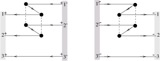
Figure 14: Time ordered graphs of the unconnected irreducible two-particle kernel $U_{M}^{(2)}$ as defined in eq. (4.4). Here only the term (12)3 is shown.

Secondly, we find a connected part $C_{M}^{(2)}$ that contains the sum of all possible irreducible quark-exchange diagrams. This term is given by

$$C_{M}^{(2)} := -{\rm i}\;{h_{0}}_{M}\;\bigg{[}\Lambda\left\langle{G_{0}}_{M}\;K^{12}_{M}\;{G_{0}}_{M}\;K^{23}_{M}\;{G_{0}}_{M}\right\rangle\overline{\Lambda}$$ (201)

$$\phantom{-{\rm i}\;{h_{0}}_{M}\;\bigg{[}\bigg{.}}-\Lambda\left\langle{G_{0}}_{M}\;K^{12}_{M}\;{G_{0}}_{M}\right\rangle\overline{\Lambda}\;{h_{0}}_{M}\;\Lambda\left\langle{G_{0}}_{M}\;K^{23}_{M}\;{G_{0}}_{M}\right\rangle\overline{\Lambda}\;\bigg{]}\;{h_{0}}_{M}{}$$

$$+\quad\begin{array}[]{l}\textrm{corresponding terms with other quark pairings in the incoming and}\\ \textrm{outgoing channels: (23, 12), (12, 31), (31, 12), (31, 23) and (23, 31)}\end{array}$$

In fig. 15 the different time-ordered graphs contributing to the irreducible second order quark-exchange interaction are shown diagrammatically.

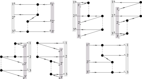
Figure 15: Time ordered graphs of the connected irreducible quark-exchange interaction $C_{M}^{(2)}$ as defined in eq. (201). As an example only term (12, 23) is shown.

The explicit calculation of the second order terms $\Lambda\langle{G_{0}}_{M}\;\overline{K}^{(2)}_{M}\;{G_{0}}_{M}\;\overline{K}^{(2)}_{M}\;{G_{0}}_{M}\rangle\overline{\Lambda}$, needed for the determination of $U_{M}^{(2)}$ and $C_{M}^{(2)}$, is lengthy but straightforward and can be performed by making again elaborate use of the residue theorem. Owing to the increasing number of quark-lines and the increasing number of contributing poles in the relative energy variables $p_{\xi}^{0}$ and $p_{\eta}^{0}$, the structure and coordinate dependence of these explicit expressions is rather complicated in comparison to the rather simple structure of the Born term (192). Moreover $U_{M}^{(2)}$ and $C_{M}^{(2)}$ exhibit an explicit $M$-dependence. We restrict our explicit calculations to the leading Born term (Born approximation).

5 Bound-states in Born approximation of the quasi-potential

The discussion of the lowest order contributions to the effective quasi-potential ${V^{\rm eff}_{M}}$ in the last section clearly showed that with increasing order of the contributions to ${V^{\rm eff}_{M}}$ the explicit expressions rapidly become more complicated. While the dominant leading order Born term ${{V^{\rm eff}_{M}}}^{(1)}$ is still rather simple in structure, already the second order contribution ${{V^{\rm eff}_{M}}}^{(2)}$ contains a lot of different irreducible terms whose structure is quite complex and thus impedes an efficient numerical treatment. Therefore, expecting these contributions to be small in comparison to the leading Born term, we consider the Born approximation

$${V^{\rm eff}_{M}}\simeq{V^{\rm eff}_{M}}^{(1)}$$ (202)

only. For the sake of completeness let us summarize the corresponding expressions for the Salpeter equation and the normalization condition in this approximation. These equations shall constitute the basis of our quark model for baryons.

5.1 Salpeter equation and normalization condition

Approximating the series (167) by the leading Born term (192), the approximated Salpeter equation (164) can still be formulated as an ordinary eigenvalue problem,

$${\cal H}\Phi_{M}^{\Lambda}=M\;\Phi_{M}^{\Lambda},$$ (203)

since, due to eq. (192), the Born term ${V^{\rm eff}_{M}}^{(1)}$ in fact is $M$-independent. The $M$-independent Salpeter Hamiltonian ${\cal H}$ then reads explicitly:

$$\left[{\cal H}\Phi_{M}^{\Lambda}\right]({\bf p_{\xi}},{\bf p_{\eta}}) = {\cal H}_{0}({\bf p_{\xi}},{\bf p_{\eta}})\;\Phi_{M}^{\Lambda}({\bf p_{\xi}},{\bf p_{\eta}})$$

$$+ \left[\Lambda_{1}^{+}({\bf p_{1}})\otimes\Lambda_{2}^{+}({\bf p_{2}})\otimes\Lambda_{3}^{+}({\bf p_{3}})+\Lambda_{1}^{-}({\bf p_{1}})\otimes\Lambda_{2}^{-}({\bf p_{2}})\otimes\Lambda_{3}^{-}({\bf p_{3}})\right]{}$$

$$\times\;\;\gamma^{0}\otimes\gamma^{0}\otimes\gamma^{0}\;\int\frac{\textrm{d}^{3}p_{\xi}^{\prime}}{(2\pi)^{3}}\;\frac{\textrm{d}^{3}p_{\eta}^{\prime}}{(2\pi)^{3}}\;V^{(3)}({\bf p_{\xi}},{\bf p_{\eta}};\;{\bf p_{\xi}^{\prime}},{\bf p_{\eta}^{\prime}})\;\Phi_{M}^{\Lambda}({\bf p_{\xi}^{\prime}},{\bf p_{\eta}^{\prime}}){}$$

$$+ \left[\Lambda_{1}^{+}({\bf p_{1}})\otimes\Lambda_{2}^{+}({\bf p_{2}})\otimes\Lambda_{3}^{+}({\bf p_{3}})-\Lambda_{1}^{-}({\bf p_{1}})\otimes\Lambda_{2}^{-}({\bf p_{2}})\otimes\Lambda_{3}^{-}({\bf p_{3}})\right]{}$$

$$\times\;\;\gamma^{0}\otimes\gamma^{0}\otimes{\rm 1\kern-3.00003ptI}\;\int\frac{\textrm{d}^{3}p_{\xi}^{\prime}}{(2\pi)^{3}}\;V^{(2)}({\bf p_{\xi}},{\bf p_{\xi}^{\prime}})\otimes{\rm 1\kern-3.00003ptI}\;\Phi_{M}^{\Lambda}({\bf p_{\xi}^{\prime}},{\bf p_{\eta}}){}$$

$$+ \textrm{corresponding terms with interacting quark pairs (23) and (31)}.$$

Note the striking structural difference between the connected three-body part and the unconnected two-body part: The two body term shows a relative sign between the positive and negative energy projectors and occurrence of the identity (instead of $\gamma^{0}$) in the Dirac space of the spectator quark.

To be consistent, the same approximation of ${V^{\rm eff}_{M}}$ must also be used in the normalization condition (187). In Born approximation, the second term in the normalization condition (187) vanishes, owing to the explicit $M$-independence of the Born term ${V^{\rm eff}_{M}}^{(1)}$ and we arrive at

$$\frac{\partial}{\partial M}\;{V^{\rm eff}_{M}}^{(1)}=0\quad\Rightarrow\quad\langle\Phi_{M}^{\Lambda}|\Phi_{M}^{\Lambda}\rangle\;\;=\;\;2M.$$ (205)

Consequently, the solutions $\Phi^{\Lambda}_{M}$ of the Salpeter equation (5.1) in Born approximation of ${V^{\rm eff}_{M}}$ have to fulfill the same ${\cal L}^{2}$-normalization condition (112) as in the case where the dynamics was determined by the instantaneous three-body kernel alone (see subsect. 4.3.3), i.e.

$$\langle\Phi_{M}^{\Lambda}|\Phi_{M}^{\Lambda}\rangle=\int\frac{\textrm{d}^{3}p_{\xi}}{(2\pi)^{3}}\;\frac{\textrm{d}^{3}p_{\eta}}{(2\pi)^{3}}\;\sum_{a_{1},a_{2},a_{3}}{\Phi_{M}^{\Lambda}}_{a_{1}a_{2}a_{3}}^{*}({\bf p_{\xi}},{\bf p_{\eta}})\;{\Phi_{M}^{\Lambda}}_{a_{1}a_{2}a_{3}}({\bf p_{\xi}},{\bf p_{\eta}})=2M.$$ (206)

The Salpeter equation for $\Phi_{M}^{\Lambda}$ and the corresponding adjoint equation for $\overline{\Phi}_{M}^{\Lambda}$ must be consistent with the relation (186) between $\Phi_{M}^{\Lambda}$ and $\overline{\Phi}_{M}^{\Lambda}$. This leads to the following condition for the instantaneous interaction kernels $V^{(3)}$ and $V^{(2)}$,

$$\gamma^{0}\otimes\gamma^{0}\otimes\gamma^{0}\;\left[{V^{(3)}}({\bf p_{\xi}^{\prime}},{\bf p_{\eta}^{\prime}};\;{\bf p_{\xi}},{\bf p_{\eta}})\right]^{\dagger}\;\gamma^{0}\otimes\gamma^{0}\otimes\gamma^{0} \stackrel{{\scriptstyle!}}{{=}} V^{(3)}({\bf p_{\xi}},{\bf p_{\eta}};\;{\bf p_{\xi}^{\prime}},{\bf p_{\eta}^{\prime}}){}$$

$$\gamma^{0}\otimes\gamma^{0}\;\left[{V^{(2)}}({\bf p_{\xi}^{\prime}},{\bf p_{\xi}})\right]^{\dagger}\;\gamma^{0}\otimes\gamma^{0} \stackrel{{\scriptstyle!}}{{=}} V^{(2)}({\bf p_{\xi}},{\bf p_{\xi}^{\prime}}),$$ (207)

which implies that the Salpeter Hamiltonian (5.1) in Born approximation of the effective kernel is hermitean with respect to the scalar product $\langle\cdot|\cdot\rangle$, i.e.

$$\langle\Phi_{1}|{\cal H}\;\Phi_{2}\rangle=\langle{\cal H}\;\Phi_{1}|\Phi_{2}\rangle\quad\forall\quad\Phi_{1},\Phi_{2}\quad\textrm{with}\quad\Lambda\Phi_{1,2}=\Phi_{1,2}$$ (208)

As in the case of vanishing two-quark kernels this again guarantees that

• the eigenvalues (bound-state masses) $M$ of ${\cal H}$ are real, i.e. $M^{*}=M$;

• the Salpeter amplitudes $\Phi^{\Lambda}_{M_{1}}$ and $\Phi^{\Lambda}_{M_{2}}$ corresponding to different eigenvalues $M_{1}\not=M_{2}$ are mutually orthogonal: $\langle\Phi^{\Lambda}_{M_{1}}|\Phi^{\Lambda}_{M_{2}}\rangle=0$.

5.2 Symmetries of the Salpeter equation

So far we discussed the constraints (207) of the instantaneous two- and three-quark interaction kernels $V^{(3)}$ and $V^{(2)}$ that followed from the interconnection of the amplitude $\Phi^{\Lambda}_{M}$ and its adjoint $\overline{\Phi}^{\Lambda}_{M}$ and guarantee the hermiticity of the Salpeter Hamiltonian ${\cal H}$ with respect to the positive definite scalar product $\langle\cdot|\cdot\rangle$. We are led to further conditions on the kernels if we regard the symmetries which the strong interaction of the quarks has to respect. Since the underlying theory, quantum chromodynamics (QCD), is invariant under parity transformations (${\cal P}$), time-reversal (${\cal T}$) and charge conjugation (${\cal C}$), these symmetry properties must be incorporated in the Salpeter equation. This means specifically: If $\Phi^{\Lambda}_{M}$ is a solution of the Salpeter equation, the same must also hold for ${\cal D}\;\Phi^{\Lambda}_{M}$ with ${\cal D}\in\{{\cal P},{\cal T},{\cal C}\}$ the representation of the corresponding transformation on the (projected) Salpeter amplitudes $\Phi^{\Lambda}_{M}=\Lambda\Phi_{M}$. Below we shall investigate the corresponding constraints on the interaction kernels $V^{(3)}$ and $V^{(2)}$ that follow from these invariance conditions. Instead of ${\cal P}$, ${\cal T}$ and ${\cal C}$ we alternatively consider ${\cal P}$, ${\cal T}$ and ${\cal CPT}$.

5.2.1 Parity invariance

The representation of the parity transformation ${\cal P}(x^{0},{\bf x}):=(x^{0},{\bf-x})$ on the full momentum space Salpeter amplitudes $\Phi_{M}$ is given by

$$\left[{\cal P}\Phi_{M}\right]({\bf p_{\xi}},{\bf p_{\eta}})=\gamma^{0}\otimes\gamma^{0}\otimes\gamma^{0}\;\Phi_{M}({\bf-p_{\xi}},{\bf-p_{\eta}}).$$ (209)

Owing to the intertwining relation $\Lambda^{\pm}_{i}({\bf p_{i}})\gamma^{0}=\gamma^{0}\Lambda^{\pm}_{i}({-\bf p_{i}})$ the different energy components of $\Phi_{M}$ represent invariant subspaces under the parity transformation ${\cal P}$, such that ${\cal P}$ decomposes into irreducible representations on these different subspaces. In particular, the Salpeter projector $\Lambda$ commutes with ${\cal P}$, i.e $[{\cal P},\;\Lambda]=0$ such that

$$\left[{\cal P}\Phi_{M}^{\Lambda}\right]({\bf p_{\xi}},{\bf p_{\eta}})=\gamma^{0}\otimes\gamma^{0}\otimes\gamma^{0}\;\Phi_{M}^{\Lambda}({\bf-p_{\xi}},{\bf-p_{\eta}})\quad\textrm{with}\quad\Lambda\;{\cal P}\Phi_{M}^{\Lambda}={\cal P}\Phi_{M}^{\Lambda}$$ (210)

is the representation of ${\cal P}$ on the projected Salpeter amplitudes $\Phi_{M}^{\Lambda}=\Lambda\Phi_{M}$, which actually appear in the Salpeter equation (203). Parity invariance implies that with $\Phi_{M}^{\Lambda}$ also ${\cal P}\Phi_{M}^{\Lambda}$ is a solution of the Salpeter equation, i.e. the Salpeter Hamiltonian has to commute with the representation ${\cal P}$ of the parity transformation, i.e. $\left[{\cal P},\;{\cal H}\right]=0$. With $[{\cal P},\;\Lambda]=0$ and the invariance of the free Hamiltonian ${\cal H}_{0}$ under ${\cal P}$, i.e $[{\cal P},\;{\cal H}_{0}]=0$, one readily deduces the following conditions for the three- and two-quark interaction kernels:

$$\gamma^{0}\otimes\gamma^{0}\otimes\gamma^{0}\;{V^{(3)}}(-{\bf p_{\xi}},-{\bf p_{\eta}};\;-{\bf p_{\xi}^{\prime}},-{\bf p_{\eta}^{\prime}})\;\gamma^{0}\otimes\gamma^{0}\otimes\gamma^{0} \stackrel{{\scriptstyle!}}{{=}} V^{(3)}({\bf p_{\xi}},{\bf p_{\eta}};\;{\bf p_{\xi}^{\prime}},{\bf p_{\eta}^{\prime}}),{}$$

$$\gamma^{0}\otimes\gamma^{0}\;V^{(2)}(-{\bf p_{\xi}},-{\bf p_{\xi}^{\prime}})\;\gamma^{0}\otimes\gamma^{0} \stackrel{{\scriptstyle!}}{{=}} V^{(2)}({\bf p_{\xi}},{\bf p_{\xi}^{\prime}}).$$ (211)

As usual, $\left[{\cal P},\;{\cal H}\right]=0$ also implies that the solutions $\Phi^{\Lambda}_{M}$ of the Salpeter equation simultaneously are eigenstates of ${\cal P}$, i.e.

$${\cal P}\Phi^{\Lambda}_{M,\;\pi}=\pi\;\Phi^{\Lambda}_{M,\;\pi},$$ (212)

with definite parity $\pi=\pm 1$.

5.2.2 Time-reversal invariance

The representation of the time-reversal transformation ${\cal T}(x^{0},{\bf x}):=(-x^{0},{\bf x})$ on the full momentum space Salpeter amplitudes reads

$$\left[{\cal T}\Phi_{M}\right]({\bf p_{\xi}},{\bf p_{\eta}})=-\gamma^{1}\gamma^{3}\otimes\gamma^{1}\gamma^{3}\otimes\gamma^{1}\gamma^{3}\;\Phi_{M}^{*}({\bf-p_{\xi}},{\bf-p_{\eta}}).$$ (213)

Again the different energy components of $\Phi_{M}$ define invariant subspaces under the time-reversal transformation according to the intertwining relation $\Lambda^{\pm}_{i}({\bf p_{i}})\;\gamma^{1}\gamma^{3}=\gamma^{1}\gamma^{3}\;{\Lambda^{\pm}_{i}}^{*}({-\bf p_{i}})$. In particular, we find that the Salpeter projector is time-reversal invariant, i.e. $[{\cal T},\;\Lambda]=0$, such that we have a representation of the time-reversal transformation on the subspace of purely positive and negative components, i.e. for the projected amplitudes $\Phi_{M}^{\Lambda}=\Lambda\Phi_{M}$ holds:

$$\left[{\cal T}\Phi_{M}^{\Lambda}\right]({\bf p_{\xi}},{\bf p_{\eta}})=-\gamma^{1}\gamma^{3}\otimes\gamma^{1}\gamma^{3}\otimes\gamma^{1}\gamma^{3}\;{\Phi_{M}^{\Lambda}}^{*}({\bf-p_{\xi}},{\bf-p_{\eta}})\quad\textrm{with}\quad\Lambda\;{\cal T}\Phi_{M}^{\Lambda}={\cal T}\Phi_{M}^{\Lambda}.$$ (214)

To respect time-reversal invariance of the strong interaction, we must impose that $\left[{\cal T},\;{\cal H}\right]=0$. Using the invariance property $[{\cal T},\;\Lambda]=0$ of $\Lambda$ and the time-reversal invariance of the free Hamiltonian ${\cal H}_{0}$, i.e. $[{\cal T},\;{\cal H}_{0}]=0$ we end up with the conditions

$$-\gamma^{1}\gamma^{3}\!\otimes\!\gamma^{1}\gamma^{3}\!\otimes\!\gamma^{1}\gamma^{3}\;{V^{(3)}}^{*}\!\!(-{\bf p_{\xi}},-{\bf p_{\eta}};-{\bf p_{\xi}^{\prime}},-{\bf p_{\eta}^{\prime}})\;\gamma^{1}\gamma^{3}\!\otimes\!\gamma^{1}\gamma^{3}\!\otimes\!\gamma^{1}\gamma^{3}\; \stackrel{{\scriptstyle!}}{{=}} V^{(3)}({\bf p_{\xi}},{\bf p_{\eta}};{\bf p_{\xi}^{\prime}},{\bf p_{\eta}^{\prime}}),{}$$

$$\gamma^{1}\gamma^{3}\otimes\gamma^{1}\gamma^{3}\;{V^{(2)}}^{*}(-{\bf p_{\xi}},-{\bf p_{\xi}^{\prime}})\;\gamma^{1}\gamma^{3}\otimes\gamma^{1}\gamma^{3} \stackrel{{\scriptstyle!}}{{=}} V^{(2)}({\bf p_{\xi}},{\bf p_{\xi}^{\prime}}).$$ (215)

5.2.3 ${\cal CPT}$-symmetry – Interpretation of negative bound-state masses

The Salpeter Hamiltonian ${\cal H}$ being hermitean with respect to the positive definite scalar product (113) guarantees that the eigenvalues $M$, i.e. the bound-state masses, are real, as one imposes for physically acceptable solutions. However, ${\cal H}$ is not positive definite, since even the free Hamiltonian ${\cal H}_{0}$ is not positive. Accordingly, ${\cal H}$ in general possesses both positive and negative eigenvalues and the spectrum might be even unbound from below. These negative eigenvalues, at first face seem physically unacceptable and the corresponding amplitudes also contradict the normalization (206) via the positive definite ${\cal L}^{2}$-norm. Nevertheless, these negative energy solutions with $M<0$ can be interpreted physically meaningful. In fact, since our covariant Salpeter approach is based on relativistic quantum field theory, it should reveal a particle-antiparticle symmetry as a characteristic feature due to ${\cal CPT}$-invariance. Accordingly, we demand that the instantaneous two- and three-quark interaction kernels commute with the Dirac-space operator $\bigotimes_{i=1}^{3}\gamma^{0}\gamma^{5}$, i.e.

$$\left[\gamma^{0}\gamma^{5}\otimes\gamma^{0}\gamma^{5}\otimes\gamma^{0}\gamma^{5},\;\;V^{(3)}({\bf p_{\xi}},{\bf p_{\eta}};\;{\bf p_{\xi}^{\prime}},{\bf p_{\eta}^{\prime}})\right] = 0$$ (216)

$$\left[\gamma^{0}\gamma^{5}\otimes\gamma^{0}\gamma^{5},\;\;V^{(2)}({\bf p_{\xi}},{\bf p_{\xi}^{\prime}})\right] = 0$$ (217)

in order to ensure that the three-quark Salpeter equation in fact respects the ${\cal CPT}$-symmetry of the strong interaction. In this manner the negative bound-state masses get a well defined physical interpretation as we will see in the following discussion. The conditions (216) and (217) on $V^{(3)}$ and $V^{(2)}$ imply that the Salpeter Hamiltonian ${\cal H}$ given in eq. (5.1) anticommutes with $\bigotimes_{i=1}^{3}\gamma^{0}\gamma^{5}$, i.e.

$$\left\{\gamma^{0}\gamma^{5}\otimes\gamma^{0}\gamma^{5}\otimes\gamma^{0}\gamma^{5},\;{\cal H}\right\}=0$$ (218)

as can easily be shown with the anticommutator and intertwining relations

$$\left\{\gamma^{0}\gamma^{5},\;\gamma^{0}\right\}=0,\quad\left\{\gamma^{0}\gamma^{5},\;H_{i}({\bf p_{i}})\right\}=0\quad\textrm{and}\quad\gamma^{0}\gamma^{5}\;\Lambda_{i}^{\pm}({\bf p_{i}})=\Lambda_{i}^{\mp}({\bf p_{i}})\;\gamma^{0}\gamma^{5}.$$ (219)

Moreover, it follows from (219) that $\gamma^{0}\otimes\gamma^{0}\otimes\gamma^{0}$ and hence also the representation ${\cal P}$ of the parity transformation (209) anticommutes with $\bigotimes_{i=1}^{3}\gamma^{0}\gamma^{5}$:

$$\left\{\gamma^{0}\gamma^{5}\otimes\gamma^{0}\gamma^{5}\otimes\gamma^{0}\gamma^{5},\;{\cal P}\right\}=0.$$ (220)

Now let $\Phi_{-M,\;\pi}^{\Lambda}$ be a solution of the Salpeter equation with negative mass $-M<0$ and parity $\pi$ which obeys:

$${\cal H}\;\Phi_{-M,\;\pi}^{\Lambda}=-M\;\Phi_{-M,\;\pi}^{\Lambda},\quad{\cal P}\;\Phi_{-M,\;\pi}^{\Lambda}=\pi\;\Phi_{-M,\;\pi}^{\Lambda}.$$ (221)

We consider the transformation $\Phi_{-M,\;\pi}^{\Lambda}\mapsto\widetilde{\Phi}_{-M,\;\pi}^{\Lambda}$ of the amplitude $\Phi_{-M,\;\pi}^{\Lambda}$, given by

$$\widetilde{\Phi}_{-M,\;\pi}^{\Lambda}({\bf p_{\xi}},{\bf p_{\eta}}):=\gamma^{0}\gamma^{5}\otimes\gamma^{0}\gamma^{5}\otimes\gamma^{0}\gamma^{5}\;\Phi_{-M,\;\pi}^{\Lambda}({\bf p_{\xi}},{\bf p_{\eta}}).$$ (222)

Then, due to eq. (218), also this ${\cal CPT}$-transformed amplitude $\widetilde{\Phi}_{-M,\;\pi}^{\Lambda}$ is a solution of the Salpeter equation, but now with the positive bound-state mass $+M>0$. At the same time eq. (220) implies that $\widetilde{\Phi}_{-M,\;\pi}^{\Lambda}$ has parity $-\pi$ opposite to $\Phi_{-M,\;\pi}^{\Lambda}$. Thus, we have

$${\cal H}\;\widetilde{\Phi}_{-M,\;\pi}^{\Lambda}=+M\;\widetilde{\Phi}_{-M,\;\pi}^{\Lambda}\quad{\cal P}\;\widetilde{\Phi}_{-M,\;\pi}^{\Lambda}=-\pi\;\widetilde{\Phi}_{-M,\;\pi}^{\Lambda}$$ (223)

Consequently, the eigenvalues come in pairs with opposite sign, but with eigenfunctions (Salpeter amplitudes) having opposite parity. This symmetry indeed allows the interpretation of the negative energy solutions for a given set of quantum numbers as antibaryon states, which after the transformation $\Phi_{-M,\;\pi}^{\Lambda}\mapsto\widetilde{\Phi}_{-M,\;\pi}^{\Lambda}$ yield positive energy solutions of opposite parity but otherwise with the same quantum numbers:

$$\widetilde{\Phi}_{-M,\;\pi}^{\Lambda}=\bigotimes_{i=1}^{3}\gamma^{0}\gamma^{5}\;\Phi_{-M,\;\pi}^{\Lambda}\;\;\equiv\;\;\Phi_{M,\;-\pi}^{\Lambda}.$$ (224)

This is a new interesting feature of our Salpeter equation-based baryon model in contrast to nonrelativistic (or relativized) quark potential models, which are usually based on the ordinary Schrödinger equation: Solving the Salpeter equation for fixed spin $J$ yields at the same time both the positive and the negative parity bound state spectrum of the baryons, see fig. 16 for a diagrammatical illustration of this feature. Furthermore the positive and negative parity states are coupled in this way and are not independent as in the ordinary nonrelativistic potential models.

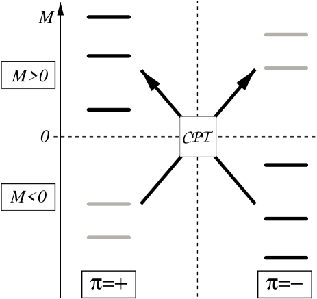
Figure 16: Interpretation of the negative energy solutions due to the ${\cal CPT}$-symmetry of the Salpeter equation represented by eq. (224). See text for explanation.

Notice that, owing to the intertwining relation $\gamma^{0}\gamma^{5}\;\Lambda_{i}^{\pm}({\bf p_{i}})=\Lambda_{i}^{\mp}({\bf p_{i}})\;\gamma^{0}\gamma^{5}$, the roles of the positive and negative energy components are interchanged by the ${\cal CPT}$-transformation:

$$\Phi_{M,\;-\pi}^{+++}\;=\;\bigotimes_{i=1}^{3}\gamma^{0}\gamma^{5}\;\;\Phi_{-M,\;\pi}^{---}\quad\textrm{and}\quad\Phi_{M,\;-\pi}^{---}\;=\;\bigotimes_{i=1}^{3}\gamma^{0}\gamma^{5}\;\;\Phi_{-M,\;\pi}^{+++}.$$ (225)

Consequently, only both subspaces of purely positive and negative energy components together (but not separately) define an invariant subspace under the ${\cal CPT}$-transformation. Thus really both subspaces are necessary to get an (irreducible) representation of ${\cal CPT}$. In particular the so-called reduced Salpeter equation, in which the negative components are a priori neglected (Tamm-Dancoff approximation), violates in general the ${\cal CPT}$-symmetry.

5.3 Eigenstates of the Salpeter projector

Let us come back to the specific projector structure of the Salpeter equation and discuss in some more detail the corresponding induced structure of the solutions, i.e. of the (projected) Salpeter amplitudes $\Phi_{M}^{\Lambda}=\Lambda\Phi_{M}$, which obviously are eigenstates of the Salpeter projector. These projection properties of the solutions reduce the number of independent functions necessary to describe the baryon state. Due to the form of the Salpeter projector $\Lambda$ the solutions split into the two orthogonal purely positive and purely negative energy components and thus the (in Dirac space) 64-component function in fact reduces to an effectively 16-component function only. To perform this reduction of the Salpeter amplitude to a 16-component function we have to determine the general form of the eigenstates of the Salpeter projector $\Lambda$. To this end we will consider first the positive and negative energy solutions of the free Dirac equation for a spin-$1/2$ particle. These four-component Dirac spinors, which are the eigenstates of the energy projectors $\Lambda^{\pm}$, can be constructed in the usual way by the embedding map of two-component Pauli spinors. This scheme can then be generalized to the (projected) three-fermion Salpeter amplitudes $\Phi_{M}^{\Lambda}$ which are eigenstates of the Salpeter projector $\Lambda$ and accordingly are formed by a three-fermion embedding map.

For the following considerations it is convenient to adjust our notation to the symmetry properties of the Salpeter amplitude under permutations of the quarks, especially in the case of different quark masses. So far we used a simplified notation suppressing the flavor dependencies of the single-quark operators $H_{i}$ and $\Lambda^{\pm}_{i}$ and we assigned to each quark $i$ an individual quark mass $m_{i}$. With the replacements of $H_{i}$ and $\Lambda^{\pm}_{i}$ given by

$$H({\bf p_{i}}) := \sum_{f}\;H_{m_{f}}({\bf p_{i}})\otimes{\cal P}^{\cal F}_{f},\quad\textrm{with}\quad H_{m_{f}}({\bf p}):=\gamma^{0}\;({\mbox{\boldmath$\gamma$}\cdot p}+m_{f})$$ (226)

$$\Lambda^{\pm}({\bf p_{i}}) := \sum_{f}\;\Lambda^{\pm}_{m_{f}}({\bf p_{i}})\otimes{\cal P}^{\cal F}_{f},\quad\textrm{with}\quad\Lambda_{m_{f}}^{\pm}({\bf p}):=\frac{\omega_{m_{f}}({\bf p})\pm H_{m_{f}}({\bf p})}{2\omega_{m_{f}}({\bf p})}$$ (228)

$$\phantom{\sum_{f}\;\Lambda^{\pm}_{m_{f}}({\bf p_{i}})\otimes{\cal P}^{\cal F}_{f},}\quad\;\textrm{and}\;\;\quad\omega_{m_{f}}({\bf p}):=\sqrt{|{\bf p}|^{2}+m_{f}^{2}},$$

the correct assignment of quark masses according to their flavor $f=u,d,s$ is realized by the flavor projectors ${\cal P}^{\cal F}_{f}:=|f\rangle\langle f|$ such that the free Hamiltonian ${\cal H}_{0}$ and the Salpeter projector

$$\Lambda({\bf p_{\xi}},{\bf p_{\eta}}) = \Lambda^{+++}({\bf p_{\xi}},{\bf p_{\eta}})+\Lambda^{---}({\bf p_{\xi}},{\bf p_{\eta}}),$$ (229)

$$\Lambda^{\pm\pm\pm}({\bf p_{\xi}},{\bf p_{\eta}}) := \Lambda^{\pm}({\bf p_{1}})\otimes\Lambda^{\pm}({\bf p_{2}})\otimes\Lambda^{\pm}({\bf p_{3}})$$ (230)

become permutationally invariant operators.

5.3.1 Dirac spinors as embedded Pauli spinors

Let us first consider the Dirac spinors $\psi_{m}^{\pm}:\textrm{R}_{m}^{\pm}\rightarrow{\mathchoice{{\rm C\kern-3.99994pt\raisebox{0.0pt}{\rule{0.21529pt}{6.69998pt}}\kern 3.99994pt}}{{\rm C\kern-3.99994pt\raisebox{0.12915pt}{\rule{0.21529pt}{6.69998pt}}\kern 3.99994pt}}{{\rm C\kern-3.00003pt\raisebox{0.25832pt}{\rule{0.21529pt}{4.49997pt}}\kern 3.00003pt}}{{\rm C\kern-3.00003pt\raisebox{0.25832pt}{\rule{0.21529pt}{3.00003pt}}\kern 3.00003pt}}}^{4}$ for a single spin-$1/2$ particle with mass $m$, i.e. the positive and negative energy solutions of the free Dirac equation on the positive/negative mass shell $\textrm{R}_{m}^{\pm}:=\{p\in{\rm I\kern-1.99997ptR}^{4}:\langle p,p\rangle=m^{2},\;p=(\pm\omega_{m}({\bf p}),{\bf p})\}$. These are eigenstates of the positive and negative energy projectors $\Lambda_{m}^{\pm}$:

$$\Lambda_{m}^{+}({\bf p})\;\psi_{m}^{+}(p) = \psi_{m}^{+}(p)\quad\textrm{with}\quad p=(+\omega_{m}({\bf p}),{\bf p})\in\textrm{R}_{m}^{+}$$ (231)

$$\Lambda_{m}^{-}({\bf p})\;\psi_{m}^{-}(\tilde{p}) = \psi_{m}^{-}(\tilde{p})\quad\textrm{with}\quad\tilde{p}=(-\omega_{m}({\bf p}),{\bf p})\in\textrm{R}_{m}^{-}.$$ (232)

As usual, the positive and negative energy solutions $\psi_{m}^{\pm}:\textrm{R}_{m}^{\pm}\rightarrow{\mathchoice{{\rm C\kern-3.99994pt\raisebox{0.0pt}{\rule{0.21529pt}{6.69998pt}}\kern 3.99994pt}}{{\rm C\kern-3.99994pt\raisebox{0.12915pt}{\rule{0.21529pt}{6.69998pt}}\kern 3.99994pt}}{{\rm C\kern-3.00003pt\raisebox{0.25832pt}{\rule{0.21529pt}{4.49997pt}}\kern 3.00003pt}}{{\rm C\kern-3.00003pt\raisebox{0.25832pt}{\rule{0.21529pt}{3.00003pt}}\kern 3.00003pt}}}^{4}$ of the Dirac equation may be written in the Weyl representation as

$$\psi_{m}^{+}(p)\;=\;T^{+}_{m}({\bf p})\;\varphi_{m}^{+}(p)\quad\textrm{with}\quad T^{+}_{m}({\bf p}) := \frac{1}{\sqrt{2\;\omega_{m}{({\bf p})}}}\left(\begin{array}[]{c}\sqrt{\sigma({\cal P}p)}\\ \sqrt{\sigma(p)}\end{array}\right)$$ (235)

$$\psi_{m}^{-}(\tilde{p})\;=\;T^{-}_{m}({\bf p})\;\varphi_{m}^{-}(\tilde{p})\quad\textrm{with}\quad T^{-}_{m}({\bf p}) := \frac{1}{\sqrt{2\;\omega_{m}{({\bf p})}}}\left(\begin{array}[]{c}-\sqrt{\sigma(p)}\\ \sqrt{\sigma({\cal P}p)}\end{array}\right)$$ (238)

where $\varphi_{m}^{\pm}:\textrm{R}_{m}^{\pm}\rightarrow{\mathchoice{{\rm C\kern-3.99994pt\raisebox{0.0pt}{\rule{0.21529pt}{6.69998pt}}\kern 3.99994pt}}{{\rm C\kern-3.99994pt\raisebox{0.12915pt}{\rule{0.21529pt}{6.69998pt}}\kern 3.99994pt}}{{\rm C\kern-3.00003pt\raisebox{0.25832pt}{\rule{0.21529pt}{4.49997pt}}\kern 3.00003pt}}{{\rm C\kern-3.00003pt\raisebox{0.25832pt}{\rule{0.21529pt}{3.00003pt}}\kern 3.00003pt}}}^{2}$ are two-component Pauli spinors, ${\cal P}$ is the parity transformation, i.e. ${\cal P}\;p=(\omega_{m}({\bf p}),-{\bf p})$ for $p=(p^{0},{\bf p})=(\omega_{m}({\bf p}),{\bf p})$, and

$$\sigma(p):=\sigma_{\mu}\;p^{\mu}\quad\Rightarrow\quad\sqrt{\sigma(p)}=\frac{\sigma(p)+m}{\sqrt{2(\omega_{m}{({\bf p})+m)}}},$$ (239)

with $\sigma_{i}$ the Pauli matrices and $\sigma_{0}=\sigma^{0}={\rm 1\kern-3.00003ptI}_{{\mathchoice{{\rm C\kern-2.79996pt\raisebox{0.0pt}{\rule{0.1507pt}{4.68999pt}}\kern 2.79996pt}}{{\rm C\kern-2.79996pt\raisebox{0.09041pt}{\rule{0.1507pt}{4.68999pt}}\kern 2.79996pt}}{{\rm C\kern-2.10002pt\raisebox{0.18082pt}{\rule{0.1507pt}{3.14998pt}}\kern 2.10002pt}}{{\rm C\kern-2.10002pt\raisebox{0.18082pt}{\rule{0.1507pt}{2.10002pt}}\kern 2.10002pt}}}^{2}}$. We wrote these relations already in a form that defines the so-called embedding operations $T^{\pm}_{m}({\bf p}):{\mathchoice{{\rm C\kern-3.99994pt\raisebox{0.0pt}{\rule{0.21529pt}{6.69998pt}}\kern 3.99994pt}}{{\rm C\kern-3.99994pt\raisebox{0.12915pt}{\rule{0.21529pt}{6.69998pt}}\kern 3.99994pt}}{{\rm C\kern-3.00003pt\raisebox{0.25832pt}{\rule{0.21529pt}{4.49997pt}}\kern 3.00003pt}}{{\rm C\kern-3.00003pt\raisebox{0.25832pt}{\rule{0.21529pt}{3.00003pt}}\kern 3.00003pt}}}^{2}\mapsto{\mathchoice{{\rm C\kern-3.99994pt\raisebox{0.0pt}{\rule{0.21529pt}{6.69998pt}}\kern 3.99994pt}}{{\rm C\kern-3.99994pt\raisebox{0.12915pt}{\rule{0.21529pt}{6.69998pt}}\kern 3.99994pt}}{{\rm C\kern-3.00003pt\raisebox{0.25832pt}{\rule{0.21529pt}{4.49997pt}}\kern 3.00003pt}}{{\rm C\kern-3.00003pt\raisebox{0.25832pt}{\rule{0.21529pt}{3.00003pt}}\kern 3.00003pt}}}^{4}$. They map arbitrary two-component Pauli spinors $\varphi_{m}^{\pm}$ into four-component orthogonal eigenstates $\psi_{m}^{\pm}$ of the energy projectors $\Lambda_{m}^{\pm}$. This is also apparent from the properties $\Lambda_{m}^{\pm}({\bf p})\;T^{\pm}_{m}({\bf p})=T^{\pm}_{m}({\bf p})$ and $\Lambda_{m}^{\mp}({\bf p})\;T^{\pm}_{m}({\bf p})=0$ of these embedding maps. On the other hand the mappings $\psi_{m}^{\pm}\leftrightarrow\varphi_{m}^{\pm}$ are also unique, since they satisfy

$$\left[T^{\pm}_{m}({\bf p})\right]^{\dagger}\;T^{\pm}_{m}({\bf p})={\rm 1\kern-3.00003ptI}_{{\mathchoice{{\rm C\kern-2.79996pt\raisebox{0.0pt}{\rule{0.1507pt}{4.68999pt}}\kern 2.79996pt}}{{\rm C\kern-2.79996pt\raisebox{0.09041pt}{\rule{0.1507pt}{4.68999pt}}\kern 2.79996pt}}{{\rm C\kern-2.10002pt\raisebox{0.18082pt}{\rule{0.1507pt}{3.14998pt}}\kern 2.10002pt}}{{\rm C\kern-2.10002pt\raisebox{0.18082pt}{\rule{0.1507pt}{2.10002pt}}\kern 2.10002pt}}}^{2}}\quad\textrm{and thus}\quad\varphi_{m}^{\pm}={T^{\pm}_{m}}^{\dagger}\;\psi_{m}^{\pm}$$ (240)

and, in particular, they are isometric operations: ${\psi_{m}^{\pm}}^{\dagger}\psi_{m}^{\pm}={\varphi_{m}^{\pm}}^{\dagger}\varphi_{m}^{\pm}$. Finally, we define single-quark embedding operations

$$T^{\pm}({\bf p}):=\sum_{f}\;T^{\pm}_{m_{f}}({\bf p})\otimes{\cal P}^{\cal F}_{f}$$ (241)

which account for the correct mass assignment for each flavor $f$ and accordingly map to eigenstates of the energy projectors $\Lambda^{\pm}({\bf p})$ defined in eq. (228):

$$\Lambda^{\pm}({\bf p})\;T^{\pm}({\bf p})=T^{\pm}({\bf p})\quad\textrm{and}\quad\Lambda^{\mp}({\bf p})\;T^{\pm}({\bf p})=0$$ (242)

5.3.2 Embedding map for Salpeter amplitudes $\Phi_{M}^{\Lambda}$

Now we use this result for the construction of the solutions

$$\Phi_{M}^{\Lambda}({\bf p_{\xi}},{\bf p_{\eta}})=\Phi_{M}^{+++}({\bf p_{\xi}},{\bf p_{\eta}})+\Phi_{M}^{---}({\bf p_{\xi}},{\bf p_{\eta}})$$ (243)

of the Salpeter equation, whose components

$$\Phi_{M}^{\pm\pm\pm}({\bf p_{\xi}},{\bf p_{\eta}})\;=\;\Lambda^{\pm\pm\pm}({\bf p_{\xi}},{\bf p_{\eta}})\;\Phi_{M}({\bf p_{\xi}},{\bf p_{\eta}})$$ (244)

are eigenstates of the positive and negative energy projectors $\Lambda^{\pm\pm\pm}$. According to the above discussion we now define the three-quark embedding maps by the tensor products of single quark embedding operators (241)

$$T^{\pm\pm\pm}({\bf p_{\xi}},{\bf p_{\eta}}):=T^{\pm}({\bf p_{1}})\otimes T^{\pm}({\bf p_{2}})\otimes T^{\pm}({\bf p_{3}}).$$ (245)

Then the positive and negative energy contributions $\Phi_{M}^{\pm\pm\pm}$ to $\Phi_{M}^{\Lambda}$ can be uniquely written as

$$\Phi_{M}^{\pm\pm\pm}({\bf p_{\xi}},{\bf p_{\eta}})\;=\;T^{\pm\pm\pm}({\bf p_{\xi}},{\bf p_{\eta}})\;\varphi_{M}^{\pm}({\bf p_{\xi}},{\bf p_{\eta}})$$ (246)

in terms of the embedded three-particle amplitudes $\varphi_{M}^{\pm}$ which involve triple tensor products of Pauli spinors only. Finally, we have for the Salpeter amplitude $\Phi_{M}^{\Lambda}$ the unique orthogonal decomposition

$$\Phi_{M}^{\Lambda}({\bf p_{\xi}},{\bf p_{\eta}})=T^{+++}({\bf p_{\xi}},{\bf p_{\eta}})\;\varphi_{M}^{+}({\bf p_{\xi}},{\bf p_{\eta}})\;+\;T^{---}({\bf p_{\xi}},{\bf p_{\eta}})\;\varphi_{M}^{-}({\bf p_{\xi}},{\bf p_{\eta}})$$ (247)

and thus the determination of the (in Dirac space originally $4\otimes 4\otimes 4=$) 64-component solution $\Phi_{M}^{\Lambda}$ of the Salpeter equation reduces via the embedding map to finding the two (only $2\otimes 2\otimes 2=$) 8-component amplitudes $\varphi_{M}^{\pm}$. Due to the isometry of the embedding maps $T^{\pm\pm\pm}$ which follows from eq. (240), the normalization condition for the Salpeter amplitudes $\Phi_{M}^{\Lambda}$ can be expressed in terms of these Pauli-spinors $\varphi_{M}^{\pm}$ according to

$$\langle\Phi_{M}^{\Lambda}|\Phi_{M}^{\Lambda}\rangle\;\;=\;\;\langle\varphi_{M}^{+}|\varphi_{M}^{+}\rangle+\langle\varphi_{M}^{-}|\varphi_{M}^{-}\rangle\;\;=\;\;2M,$$ (248)

where $\langle\varphi_{M}^{\pm}|\varphi_{M}^{\pm}\rangle$ denotes the usual nonrelativistic (positive definite) $\mathcal{L}^{2}$ norm. The next step is to investigate the structure of these three-quark Pauli amplitudes for a given set of quantum numbers specifying a baryon, in order to find a proper basis.

5.4 General decomposition of the Salpeter amplitudes

The three-quark Salpeter amplitude $\Phi^{\Lambda}_{M}$ of a baryon is characterized by a set of quantum numbers that are conserved under the strong interaction. We consider in this work light baryons, which are built up by quarks with flavors up (u), down (d) and strange (s). The flavor-$SU(3)$ symmetry is explicitly broken to $SU(2)\otimes U(1)$ by the different constituent quark masses $m_{u}=m_{d}<m_{s}$. With $m_{u}=m_{d}\equiv m_{n}$ only the $SU(2)$ isospin symmetry shall be assumed to be exact. Due to parity invariance, rotational invariance and this (broken) flavor invariance a baryon is then characterized by the parity $\pi$, the total spin $J$ with 3-component $M_{J}$, isospin $T$ with 3-component $M_{T}$ and strangeness $S^{*}$. Moreover, according to Pauli’s principle, the (projected) Salpeter amplitude, together with its positive and negative energy components, must be totally antisymmetric under permutations $\sigma\in S_{3}$.

Consider the three-quark Salpeter amplitude $\Phi^{\Lambda}_{M}\equiv{\Phi^{\Lambda}_{M\;\;}}_{J^{\pi}M_{J}TM_{T}S^{*}}$ describing a baryon with the quantum numbers listed above. In order to determine the structure of its embedded Pauli spinors, we have to investigate, how the corresponding transformation properties of the Salpeter amplitude $\Phi^{\Lambda}_{M}$ transfer to the Pauli spinors $\varphi_{M}^{\pm}$ via the embedding maps $T^{+++}$ and $T^{---}$:

• The representation ${\cal P}$ of the parity transformation is given for the Salpeter amplitudes $\Phi_{M}^{\Lambda}$ by

  $$\left[{\cal P}\Phi_{M}^{\Lambda}\right]({\bf p_{\xi}},{\bf p_{\eta}})=\gamma^{0}\otimes\gamma^{0}\otimes\gamma^{0}\;\Phi_{M}^{\Lambda}({\bf-p_{\xi}},{\bf-p_{\eta}}).$$ (249)

  With our special choice (235) and (238) for the embedding operations $T_{m}^{\pm}$, we find the following simple intertwining relations

  $${\cal P}\;T^{\pm\pm\pm}=T^{\pm\pm\pm}\;\left[\pm{\cal P}^{\prime}\right].$$ (250)

  On the right hand side, $\pm{\cal P}^{\prime}$ is the corresponding induced representation for the Pauli amplitudes $\varphi^{\pm}_{M}$, where the symbol ${\cal P}^{\prime}$ is used to denote the usual nonrelativistic representation of the parity transformation, i.e.

  $$\left[{\cal P}^{\prime}\;\varphi^{\pm}_{M}\right]({\bf p_{\xi}},{\bf p_{\eta}}):=\varphi^{\pm}_{M}(-{\bf p_{\xi}},-{\bf p_{\eta}}).$$ (251)

  Hence $T^{+++}$ preserves parity, whereas $T^{---}$ reverses parity, and, consequently, for a Salpeter amplitude with parity $\pi$, i.e. ${\cal P}\Phi_{M}^{\Lambda}=\pi\;\Phi_{M}^{\Lambda}$, the positive energy Pauli amplitude has the same parity $\pi$, whereas the negative energy amplitude has the opposite parity $-\pi$:

  $${\cal P}^{\prime}\varphi^{\pm}_{M}=\pm\pi\;\varphi^{\pm}_{M}.$$ (252)

• The Salpeter amplitudes $\Phi_{M}^{\Lambda}$ transform under rotations $R_{\omega}\in SO(3)$, with rotation vector $\mbox{\boldmath$\omega$}\in{\rm I\kern-1.99997ptR}^{3}$, as

  $$\left[{\cal D}_{R_{\omega}}\;\Phi_{M}^{\Lambda}\right]({\bf p_{\xi}},{\bf p_{\eta}})=S_{u}\otimes S_{u}\otimes S_{u}\;\Phi_{M}^{\Lambda}(R_{\omega}^{-1}{\bf p_{\xi}},R_{\omega}^{-1}{\bf p_{\eta}}).$$ (253)

  In the Weyl representation we have

  $$S_{u}=\left(\begin{array}[]{cc}u&0\\ 0&u\end{array}\right)\quad\textrm{where}\quad u\;=\;\exp\;(-{\rm i}\;{\mbox{\boldmath$\sigma$}}\cdot{\mbox{\boldmath$\omega$}})\in SU(2),$$ (254)

  with $u\;\sigma(p)\;u^{\dagger}=\sigma(R_{\omega}\;p)$ and we find the intertwining relations

  $${\cal D}_{R_{\omega}}\;T^{\pm\pm\pm}=T^{\pm\pm\pm}\;{\cal D}^{\prime}_{R_{\omega}}.$$ (255)

  Here the induced representation ${\cal D}^{\prime}_{R_{\omega}}$ of $R_{\omega}$, which acts on the Pauli amplitudes $\varphi^{\pm}_{M}$, is exactly the usual nonrelativistic representation of the rotation $R_{\omega}$ for a system of three spin-$\frac{1}{2}$ fermions:

  $$\left[{\cal D}^{\prime}_{R_{\omega}}\;\varphi^{\pm}_{M}\right]({\bf p_{\xi}},{\bf p_{\eta}})=u\otimes u\otimes u\;\varphi^{\pm}_{M}(R_{\omega}^{-1}{\bf p_{\xi}},R_{\omega}^{-1}{\bf p_{\eta}}).$$ (256)

  Thus, to get the irreducible subspaces $\{J,\;M_{J}=-J,\ldots,J\}$ of ${\cal D}_{R_{\omega}}$, i.e. the Salpeter amplitudes $\Phi_{M}^{\Lambda}$ with definite total spin $J$ and 3-component $M_{J}$, the Pauli amplitudes $\varphi^{\pm}_{M}$ have simply to be the usual eigenstates of the total angular momentum operator ${\bf\hat{J}}={\bf\hat{L}}+{\bf\hat{S}}$ as in a nonrelativistic system of three spin-$\frac{1}{2}$ fermions.

• As mentioned already, the three-quark embedding operators $T^{\pm\pm\pm}$ explicitly break the flavor-$SU(3)$ symmetry by the different quark masses $m_{n}<m_{s}$ and only a $SU(2)\otimes U(1)$ invariance remains. The operators of isospin and strangeness hence commute with the embedding maps $T^{\pm\pm\pm}$, and accordingly the Pauli amplitudes $\varphi^{\pm}_{M}$ are their eigenstates with quantum numbers $T$, $M_{T}$ and $S^{*}$.

• The three-quark embedding operations $T^{\pm\pm\pm}$ apparently are completely symmetric under arbitrary permutations $\sigma\in S_{3}$ of quarks by their construction (245), i.e.

  $${\cal D}_{\sigma}\;T^{\pm\pm\pm}=T^{\pm\pm\pm}\;{\cal D}^{\prime}_{\sigma},$$ (257)

  where $\mathcal{D}_{\sigma}$ and $\mathcal{D}^{\prime}_{\sigma}$ are the representations of the permutation $\sigma\in S_{3}$ on the Salpeter and Pauli amplitudes, respectively. This is a crucial point that permits to reduce the symmetry considerations of the Salpeter amplitudes to the embedded Pauli spinors. As the baryon Salpeter amplitude $\Phi^{\Lambda}_{M}$ must be totally antisymmetric, i.e.

  $${\cal D}_{\sigma}\;\Phi_{M}^{\Lambda}=\textrm{sign}(\sigma)\;\Phi_{M}^{\Lambda}\quad\forall\sigma\in S_{3},$$ (258)

  the Pauli spinors themselves must have this symmetry:

  $${\cal D}^{\prime}_{\sigma}\;\varphi_{M}^{\pm}=\textrm{sign}(\sigma)\;\varphi_{M}^{\pm}\quad\forall\sigma\in S_{3}.$$ (259)

In summary, the relativistic baryon Salpeter amplitude ${\Phi^{\Lambda}_{M\;\;}}_{J^{\pi}M_{J}TM_{T}S^{*}}$ with specific quantum numbers $J$, $\pi$, $T$, $M_{T}$ and $S^{*}$ can be formed by embedding ordinary totally antisymmetric nonrelativistic baryon wave functions ${\varphi_{M\;}}_{J^{\pi}M_{J}TM_{T}S^{*}}$:

$${\Phi^{\Lambda}_{M\;\;}}_{J^{\pi}M_{J}TM_{T}S^{*}}({\bf p_{\xi}},{\bf p_{\eta}}) = \phantom{+\;\;}T^{+++}({\bf p_{\xi}},{\bf p_{\eta}})\;{\varphi^{+}_{M\;}}_{J^{\pi}M_{J}TM_{T}S^{*}}({\bf p_{\xi}},{\bf p_{\eta}}){}$$ (260)

$$+\;\;T^{---}({\bf p_{\xi}},{\bf p_{\eta}})\;{\varphi^{-}_{M\;}}_{J^{-\pi}M_{J}TM_{T}S^{*}}({\bf p_{\xi}},{\bf p_{\eta}})$$

To define a basis for the totally antisymmetric three-quark Salpeter amplitude we can thus proceed in the same manner as in the nonrelativistic quark model, where the baryon wave functions ${\varphi_{M\;}}_{J^{\pm\pi}M_{J}TM_{T}S^{*}}$ have the generic form

$${\varphi_{M\;}}_{J^{\pi}M_{J}TM_{T}S^{*}}({\bf p_{\xi}},{\bf p_{\eta}})\;\;=\sum_{{\cal R}_{L},{\cal R}_{S},{\cal R}_{F}}\Bigg{\{}\left\{\left[\left[\psi^{\pi}_{L}({\bf p_{\xi}},{\bf p_{\eta}})\right]_{{\cal R}_{L}}\otimes\left[\chi_{S}\right]_{{\cal R}_{S}}\right]^{J}_{M_{J}}\otimes\left[\phi^{T\;S^{*}}_{M_{T}}\right]_{{\cal R}_{F}}\right\}_{\cal S}\otimes{\cal C}_{\cal A}\Bigg{\}}_{\cal A}$$

with

• $\left[\psi^{\pi}_{L}({\bf p_{\xi}},{\bf p_{\eta}})\right]_{{\cal R}_{L}}$ the momentum space wave function with total orbital angular momentum $L$, parity $\pi$ and permutational symmetry ${\cal R}_{L}\in\{{\cal S},{\cal M}_{\cal S},{\cal M}_{\cal A},{\cal A}\}$;

• $\left[\chi_{S}\right]_{{\cal R}_{S}}$ the spin function of three Pauli spinors coupled to total spin $S$ with permutational symmetry ${\cal R}_{S}\in\{{\cal S},{\cal M}_{\cal S},{\cal M}_{\cal A}\}$;

• $\left[\phi^{T\;S^{*}}_{M_{T}}\right]_{{\cal R}_{F}}$ the flavor function with total isospin $T$, $T_{3}$-component $M_{T}$ and strangeness $S^{*}$ which is of permutational symmetry ${\cal R}_{F}\in\{{\cal S},{\cal M}_{\cal S},{\cal M}_{\cal A},{\cal A}\}$;

• ${\cal C}_{\cal A}$ the totally antisymmetric color-singlet state given by the Levi-Cività tensor: ${\cal C}_{\cal A}=\frac{1}{\sqrt{6}}\;\epsilon_{c_{1}c_{2}c_{3}}\;|c_{1}\rangle\otimes|c_{2}\rangle\otimes|c_{3}\rangle$.

The momentum space wave function $\psi^{\pi}_{L}$ and the spin function $\chi_{S}$ are coupled as usually to states of total angular momentum $J,\;M_{J}$ according to

$$\left[\left[\psi^{\pi}_{L}({\bf p_{\xi}},{\bf p_{\eta}})\right]_{{\cal R}_{L}}\otimes\left[\chi_{S}\right]_{{\cal R}_{S}}\right]^{J}_{M_{J}}=\sum_{M_{L},M_{S}}\langle LM_{L},SM_{S}|JM_{J}\rangle\;\psi^{\pi}_{LM_{L}}({\bf p_{\xi}},{\bf p_{\eta}})\;\chi_{SM_{S}}$$ (261)

with Clebsch-Gordan coefficients $\langle LM_{L},SM_{S}|JM_{J}\rangle$; the sum over the symmetries ${\cal R}_{L}$, ${\cal R}_{S}$ and ${\cal R}_{F}$ in (5.4) is such that the combined momentum-, spin-, flavor wave function is totally symmetric, ${\cal R}_{L}\otimes{\cal R}_{S}\otimes{\cal R}_{F}={\cal S}$, and, finally, the baryon amplitude becomes totally antisymmetric with the totally antisymmetric color-singlet state ${\cal C}_{\cal A}$.

Finally, let us discuss the implications of the present covariant approach with respect to the baryonic spectrum and the nonrelativistic quark model. According to the preceding discussion, the structure of the Salpeter amplitudes seems to be very similar to that usually considered in the nonrelativistic quark model: The Pauli amplitude embedded by the positive energy embedding map $T^{+++}$ is of exactly the same structure as the usual nonrelativistic wave function for a given set of quantum numbers. But note the additional negative energy contribution to the Salpeter amplitude: For a specific parity $\pi$ of the baryon the embedding operator $T^{---}$ brings also the nonrelativistic wave functions with the opposite (’wrong’) parity $-\pi$ into play (due to the different behavior of $T^{+++}$ and $T^{---}$ under parity transformations). Thus, at a first glance, our approach seems to posses a larger number of states than the nonrelativistic approach. But recall that the negative mass $(-M<0)$ solutions of the Salpeter equation can be interpreted as the antibaryon states to baryons of just the opposite parity $-\pi$, due to the ${\cal CPT}$-symmetry of the Salpeter equation. Exactly these negative mass states, which after ${\cal CPT}$ transformation become the baryon states $(M>0)$ with opposite parity, correspond to the additional states with the ’wrong’ parity $-\pi$. This feature becomes even more apparent, if we analyze the effect of the ${\cal CPT}$-transformation on the embedded Pauli wave functions. For the embedding maps we find the relations

$$\gamma^{0}\gamma^{5}\otimes\gamma^{0}\gamma^{5}\otimes\gamma^{0}\gamma^{5}\;T^{\pm\pm\pm}({\bf p_{\xi}},{\bf p_{\eta}})=\mp\;T^{\mp\mp\mp}({\bf p_{\xi}},{\bf p_{\eta}})$$ (262)

such that the ${\cal CPT}$ transformation essentially switches the embedding maps of positive and negative energy and hence also the parity. Considering the decompositions of the negative mass solution ${\Phi^{\Lambda}_{-M\;\;}}_{J^{\pi}M_{J}TM_{T}S^{*}}$

$${\Phi^{\Lambda}_{-M\;\;}}_{J^{\pi}M_{J}TM_{T}S^{*}}=T^{+++}\;{\varphi^{+}_{-M\;}}_{J^{\pi}M_{J}TM_{T}S^{*}}+T^{---}\;{\varphi^{-}_{-M\;}}_{J^{-\pi}M_{J}TM_{T}S^{*}}$$ (263)

and of its related, ${\cal CPT}$-transformed positive mass solution of opposite parity ${\Phi^{\Lambda}_{M\;\;}}_{J^{-\pi}M_{J}TM_{T}S^{*}}$

$${\Phi^{\Lambda}_{M\;\;}}_{J^{-\pi}M_{J}TM_{T}S^{*}} = T^{+++}\;{\varphi^{+}_{M\;}}_{J^{-\pi}M_{J}TM_{T}S^{*}}+T^{---}\;{\varphi^{-}_{M\;}}_{J^{\pi}M_{J}TM_{T}S^{*}}{}$$ (264)

$$= \gamma^{0}\gamma^{5}\otimes\gamma^{0}\gamma^{5}\otimes\gamma^{0}\gamma^{5}\;{\Phi^{\Lambda}_{-M\;\;}}_{J^{\pi}M_{J}TM_{T}S^{*}}$$

the ${\cal CPT}$-transformation together with the property (262) of the embedding maps then yields the following relations for the corresponding Pauli amplitudes,

$${\varphi^{+}_{M\;}}_{J^{-\pi}M_{J}TM_{T}S^{*}} = -\;{\varphi^{-}_{-M\;}}_{J^{-\pi}M_{J}TM_{T}S^{*}},{}$$

$${\varphi^{-}_{M\;}}_{J^{\pi}M_{J}TM_{T}S^{*}} = +\;{\varphi^{+}_{-M\;}}_{J^{\pi}M_{J}TM_{T}S^{*}},$$ (265)

which means that the ${\cal CPT}$-transformation just interchanges the roles of both Pauli amplitudes. Thus we find in our present covariant approach exactly the same number of states as in the nonrelativistic quark model, a feature that in general can not be taken for granted in a relativistic approach: Consider e.g. the naive flavor-$SU(3)$ quark model. To explain the lowest lying multiplet it is assumed that the ground state orbital wave function is a totally symmetric $S$-wave, the color state is completely antisymmetric and hence the spin-flavor state has to be totally symmetric, which in the nonrelativistic approximation restricts the possible multiplets to a flavor octet with spin-$1/2$ and a flavor decuplet with spin-$3/2$. In a relativistic quark model, however, the number of spin-degrees of freedom is doubled for each quark, due to the presence of the lower components, which means that in the relativistic flavor-$SU(3)$ model the number of possible symmetric spin-flavor multiplets is much higher than in the nonrelativistic approach, see e.g. BoMe79 ; Mey75 ; Ca93 ; HKM75 , in contrast to the experimental findings, which can be explained qualitatively by the naive nonrelativistic model very well. Our approach does not reveal this problem, owing to the Salpeter projector $\Lambda$ and the ${\cal CPT}$-symmetry of the Salpeter equation, which circumvents such a proliferation of the number of states. Note that this feature of our model is a direct consequence of the instantaneous approximation or, more precisely, of the instantaneous ansatz for the genuine three-body (confinement) kernel. In view of the success of nonrelativistic quark models to account for the correct number of baryon excitations we in fact consider this to be one of the main empirical arguments to use this instantaneous ansatz.

6 Summary and conclusion

In this paper we presented how a relativistically covariant constituent quark model for baryons can be constructed within the general framework of quantum field theory. We started with the basic field theoretical quantities describing bound states of three fermions – the Bethe-Salpeter amplitudes and their adjoints – which form the residua at the bound-state poles of the six-point Green’s function. The Bethe-Salpeter amplitudes, which might be considered as the covariant analogues of ’wave functions’ in the ordinary nonrelativistic approach, obey a homogeneous eight-dimensional integral equation in momentum space – the so-called Bethe-Salpeter equation. In principle, this is the basic equation for the covariant description of bound states of three quarks in the framework of QCD, i.e. solving this equation for given single quark propagators and irreducible interaction kernels the discrete spectrum of baryons is then determined by the normalization condition.

However, neither the full quark propagators nor the interaction vertices are reliably known functions in case of QCD such that reasonable phenomenological approximations for these basic ingredients of the Bethe-Salpeter equation were necessary. In order to remain as close as possible in contact with the features of the non-relativistic quark model we adopted the concept of constituent quark masses using free quark propagators with effective quark masses and the concept to describe the quark interactions by instantaneous, unretarded potentials. Although both replacements are chosen purely phenomenologically they are justified reasonably well by the apparent success of nonrelativistic potential models. As in the corresponding framework for mesons both assumptions then allowed a reduction of the full (eight-dimensional) Bethe-Salpeter equation to a reduced six-dimensional equation (Salpeter equation) in the case of instantaneous three-quark forces. In this case we obtained an equation for the reduced amplitudes (Salpeter amplitudes) with a structure quite similar to the ordinary Schrödinger equation and the normalization condition for the Bethe-Salpeter amplitudes reduced to the ordinary ${\cal L}^{2}$ normalization condition inducing a positive definite scalar product. Complications arose, when two-particle interactions appeared, since these unconnected forces within the three-body system prevented a straightforward reduction as in the case of a pure three-body interaction alone. However, a reasonable treatment of these forces within the Salpeter framework is important since in quark models the three-body confinement forces are naturally supplemented by two-body residual interactions like the one-gluon-exchange or instanton-induced forces. We presented a method how in connection with the genuine instantaneous three-body kernel a reduction to a Salpeter equation of the same structure can nevertheless be achieved by deriving an effective instantaneous three-body kernel which parameterizes all effects of the two-body interactions.

As a crucial property of the instantaneous approximation we found that it leads to a one-to-one correspondence with the states of the non-relativistic quark model, a fact which generally can not be taken for granted in relativistic approaches according to the doubling of the spin-degrees of freedom. In this respect the special projector structure of the Salpeter equation reduces the number of functions necessary to describe the bound state and thus circumvents a proliferation of the number of states: The Salpeter amplitudes, which still contain the full Dirac structure with positive and negative energy components, can be formed by an isometric embedding map of ordinary non-relativistic three-quark Pauli wave functions.

We found the appearance of the negative energy components to be related to the particle-antiparticle symmetry due to the ${\cal CPT}$ invariance: The spectrum of the Salpeter equation contains antiparticle solutions corresponding to particles with charge conjugated quantum numbers. This is a new feature of our Salpeter model for baryons and quite in contrast to ordinary nonrelativistic or relativized quark models. Solving the Salpeter equation for fixed spin $J$ yields at the same time both the positive- and negative-parity bound-state spectrum and in particular positive and negative parity states are coupled in this way and are not independent as in nonrelativistic approaches.

The fully relativistic kinematics and the formal covariance of our approach overcomes the old difficulties of nonrelativistic approaches which in fact should be completely inadequate for small constituent quark masses. We expect the three-quark Salpeter equation to provide a more reasonable framework for quark models of baryons that should be superior to other treatments such as the nonrelativistic potential model IsKa78 ; IsKa79 or its simple so-called ”relativized” extension CaIs86 . In particular it offers the possibility to investigate the effects of the full Dirac structure of residual forces like the one-gluon-exchange or instanton-induced interaction and moreover it allows for the first time a reliable test of possible assumptions concerning the Dirac structure of three-body confining forces. In two subsequent papers Loe01b ; Loe01c we will therefore investigate explicit quark models based on the purely theoretical results of this paper and present concrete calculations of the complete non-strange and strange baryon spectrum up to 3 GeV.

Appendix A Appendix: Determination of the effective kernel $V^{\rm eff}_{M}$

In this appendix we derive a prescription to construct the effective quasi potential $V^{\rm eff}_{M}$ which has been introduced in sect. 4.4. According to eq. (155), $V^{\rm eff}_{M}$ is defined by

$$\langle{\cal G}_{M}\rangle_{\Lambda}\stackrel{{\scriptstyle!}}{{=}}\Lambda\langle{\cal G}_{M}\rangle\overline{\Lambda},$$ (266)

where on the left $\langle{\cal G}_{M}\rangle_{\Lambda}$ is given by eq. (157) which defines $V^{\rm eff}_{M}$, i.e.

$$\langle{\cal G}_{M}\rangle_{\Lambda}\;\stackrel{{\scriptstyle!}}{{=}}\;\langle{G_{0}}_{M}\rangle-\textrm{i}\;\langle{G_{0}}_{M}\rangle\;V^{\rm eff}_{M}\;\langle{\cal G}_{M}\rangle_{\Lambda}$$ (267)

and on the right ${\cal G}_{M}$ is the solution of the integral equation (140) with the integral kernel $K^{\rm R}_{M}:=V^{(3)}_{\rm R}+\overline{K}^{(2)}_{M}$, i.e.

$${\cal G}_{M}={G_{0}}_{M}-\textrm{i}\;{G_{0}}_{M}\;K^{\rm R}_{M}\;{\cal G}_{M}.$$ (268)

Now the goal is to solve eq. (266) for $V^{\rm eff}_{M}$. For power counting purposes purpose we multiply the kernel $K^{\rm R}_{M}$ by a parameter $\lambda\in[0,1]$,

$$K^{\rm R}_{M}\longrightarrow\lambda\;K^{\rm R}_{M},$$ (269)

such that the Neumann series of ${\cal G}_{M}$ becomes a power series in $\lambda$, and thus

$$\Lambda\langle{\cal G}_{M}\rangle\overline{\Lambda}=\langle{G_{0}}_{M}\rangle+\sum_{k=1}^{\infty}\lambda^{k}\;\Lambda\langle{G_{0}}_{M}\underbrace{\left[-\textrm{i}\;K^{\rm R}_{M}\right]{G_{0}}_{M}\;\ldots\;\left[-\textrm{i}\;K^{\rm R}_{M}\right]{G_{0}}_{M}}_{k\;\;{\rm times}}\rangle\overline{\Lambda}.$$ (270)

The effective kernel $V^{\rm eff}_{M}$ becomes a function of $\lambda$ which is expanded into a Taylor series according to

$$V^{\rm eff}_{M}:=\sum_{k=1}^{\infty}\lambda^{k}\;{V^{\rm eff}_{M}}^{(k)}.$$ (271)

Inserting this into eq. (267) the Neumann series of $\langle{\cal G}_{M}\rangle_{\Lambda}$ yields a multiple power series in $\lambda$:

$$\left\langle{\cal G}_{M}\right\rangle_{\Lambda} = \langle{G_{0}}_{M}\rangle-{\rm i}\;\sum_{k=1}^{\infty}\lambda^{k}\;\langle{G_{0}}_{M}\rangle\;{V^{\rm eff}_{M}}^{(k)}\;\langle{G_{0}}_{M}\rangle$$

$$+ \sum_{r=2}^{\infty}\;\;\sum_{k_{1}=1}^{\infty}\;\ldots\;\sum_{k_{r}=1}^{\infty}\lambda^{k_{1}+k_{2}+\ldots+k_{r}}\;\langle{G_{0}}_{M}\rangle\left[-\textrm{i}\;{V^{\rm eff}_{M}}^{(k_{1})}\right]\langle{G_{0}}_{M}\rangle\ldots\left[-\textrm{i}\;{V^{\rm eff}_{M}}^{(k_{r})}\right]\langle{G_{0}}_{M}\rangle.$$

Collecting all terms of equal power in the third term (which is of the order $\lambda^{\geq 2}$), the multiple power series can be transformed into an ordinary series

$$\left\langle{\cal G}_{M}\right\rangle_{\Lambda} = \langle{G_{0}}_{M}\rangle-{\rm i}\;\sum_{k=1}^{\infty}\lambda^{k}\;\langle{G_{0}}_{M}\rangle\;{V^{\rm eff}_{M}}^{(k)}\;\langle{G_{0}}_{M}\rangle$$ (273)

$$+ \sum_{k=2}^{\infty}\;\;\lambda^{k}\;\;\;\sum_{r=2}^{k}\!\!\!\sum_{\footnotesize\begin{array}[]{c}k_{1},k_{2},\ldots,k_{r}<k\\ k_{1}+k_{2}+\ldots+k_{r}=k\end{array}}\!\!\!\!\!\langle{G_{0}}_{M}\rangle\left[-\textrm{i}\;{V^{\rm eff}_{M}}^{(k_{1})}\right]\langle{G_{0}}_{M}\rangle\ldots\left[-\textrm{i}\;{V^{\rm eff}_{M}}^{(k_{r})}\right]\langle{G_{0}}_{M}\rangle.$$ (276)

Finally, we insert the resulting series (270) and (273) into eq. (266) and we arrive at

$$\sum_{k=1}^{\infty}\lambda^{k}\;\langle{G_{0}}_{M}\rangle\;{V^{\rm eff}_{M}}^{(k)}\;\langle{G_{0}}_{M}\rangle\;\;=\;\;\textrm{i}\;\sum_{k=1}^{\infty}\lambda^{k}\;\Lambda\left\langle{G_{0}}_{M}\underbrace{\left[-\textrm{i}\;K^{\rm R}_{M}\right]{G_{0}}_{M}\;\ldots\;\left[-\textrm{i}\;K^{\rm R}_{M}\right]{G_{0}}_{M}}_{k\;\;{\rm times}}\right\rangle\overline{\Lambda}$$ (279)

$$-\;\textrm{i} \sum_{k=2}^{\infty}\;\;\lambda^{k}\;\;\;\sum_{r=2}^{k}\!\!\!\sum_{\footnotesize\begin{array}[]{c}k_{1},k_{2},\ldots,k_{r}<k\\ k_{1}+k_{2}+\ldots+k_{r}=k\end{array}}\!\!\!\!\!\langle{G_{0}}_{M}\rangle\left[-\textrm{i}\;{V^{\rm eff}_{M}}^{(k_{1})}\right]\langle{G_{0}}_{M}\rangle\ldots\left[-\textrm{i}\;{V^{\rm eff}_{M}}^{(k_{r})}\right]\langle{G_{0}}_{M}\rangle$$

which now enables us to solve for $V^{\rm eff}_{M}(\lambda)$ order-by-order by comparing the expansion coefficients of each power $k$ of $\lambda$. Thus, we find the following reduced terms which are irreducible with respect to $\langle{G_{0}}_{M}\rangle$:

• In lowest order, i.e. ${\bf k=1}$, we obtain the Born term ${V^{\rm eff}_{M}}^{(1)}$:

  $$\langle{G_{0}}_{M}\rangle\;{V^{\rm eff}_{M}}^{(1)}\;\langle{G_{0}}_{M}\rangle=\Lambda\left\langle{G_{0}}_{M}\;K^{\rm R}_{M}\;{G_{0}}_{M}\right\rangle\overline{\Lambda}$$ (280)

• and in $k$th order, ${\bf k\geq 2}$, we get ${V^{\rm eff}_{M}}^{(k)}$, determined by:

  $$\langle{G_{0}}_{M}\rangle\;{V^{\rm eff}_{M}}^{(k)}\;\langle{G_{0}}_{M}\rangle\;=\;\textrm{i}\;\Lambda\left\langle{G_{0}}_{M}\underbrace{\left[-\textrm{i}\;K^{\rm R}_{M}\right]{G_{0}}_{M}\;\ldots\;\left[-\textrm{i}\;K^{\rm R}_{M}\right]{G_{0}}_{M}}_{k\;\;{\rm times}}\right\rangle\overline{\Lambda}$$ (284)

  $$-\;\textrm{i}\;\sum_{r=2}^{k}\!\!\!\sum_{\footnotesize\begin{array}[]{c}k_{1},k_{2},\ldots,k_{r}<k\\ k_{1}+k_{2}+\ldots+k_{r}=k\end{array}}\!\!\!\!\!\langle{G_{0}}_{M}\rangle\left[-\textrm{i}\;{V^{\rm eff}_{M}}^{(k_{1})}\right]\langle{G_{0}}_{M}\rangle\ldots\left[-\textrm{i}\;{V^{\rm eff}_{M}}^{(k_{r})}\right]\langle{G_{0}}_{M}\rangle$$

Finally, we amputate the free Salpeter propagators $\langle{G_{0}}_{M}\rangle$ using the Hamiltonian ${h_{0}}_{M}$ with eq. (159) and thus, with the restriction (161) for $V^{\rm eff}_{M}$, we then can solve uniquely for ${V^{\rm eff}_{M}}^{(k)}$. Consequently, we get the effective kernel $V^{\rm eff}_{M}$ as the following infinite sum of irreducible interaction terms ${V^{\rm eff}_{M}}^{(k)}$:

$$V^{\rm eff}_{M}\;\;=\;\;\sum_{k=1}^{\infty}\;\;{V^{\rm eff}_{M}}^{(k)},$$ (285)

where

$${V^{\rm eff}_{M}}^{(1)} = {h_{0}}_{M}\;\Lambda\left\langle{G_{0}}_{M}\;\overline{K}^{(2)}_{M}\;{G_{0}}_{M}\right\rangle\overline{\Lambda}\;{h_{0}}_{M},$$ (286)

$${V^{\rm eff}_{M}}^{(k)} = \textrm{i}\;{h_{0}}_{M}\;\Lambda\left\langle{G_{0}}_{M}\underbrace{(-\textrm{i})\left[V^{(3)}_{\rm R}+\overline{K}^{(2)}_{M}\right]{G_{0}}_{M}\;\ldots\;(-\textrm{i})\left[V^{(3)}_{\rm R}+\overline{K}^{(2)}_{M}\right]{G_{0}}_{M}}_{k\;\;{\rm times}}\right\rangle\overline{\Lambda}\;{h_{0}}_{M}{}$$

$$-\;\textrm{i}\;\sum_{r=2}^{k}\!\!\!\!\!\sum_{\footnotesize\begin{array}[]{c}k_{1},k_{2},\ldots,k_{r}<k\\ k_{1}+k_{2}+\ldots+k_{r}=k\end{array}}\!\!\!\!\!\!\!\left[-\textrm{i}\;{V^{\rm eff}_{M}}^{(k_{1})}\right]\langle{G_{0}}_{M}\rangle\left[-\textrm{i}\;{V^{\rm eff}_{M}}^{(k_{2})}\right]\langle{G_{0}}_{M}\rangle\ldots\left[-\textrm{i}\;{V^{\rm eff}_{M}}^{(k_{r})}\right].\!\!\!{}$$ (289)

Finally, let us discuss how the instantaneous term $V^{(3)}_{\rm R}$, i.e. that part of $V^{(3)}$ that couples to the mixed energy components, enters in ${V^{\rm eff}_{M}}^{(k)}$. As we mentioned already, this part of $V^{(3)}$ appears solely in connection with $K^{(2)}_{M}$. More specifically:

1. In the Born term ${V^{\rm eff}_{M}}^{(1)}$ the isolated contribution of $V^{(3)}_{\rm R}$ vanishes due to its instantaneity and its projector property $\overline{\Lambda}V^{(3)}_{\rm R}\Lambda=0$:

   $$\left\langle{G_{0}}_{M}\;V^{(3)}_{\rm R}\;{G_{0}}_{M}\right\rangle=\left\langle{G_{0}}_{M}\right\rangle\;V^{(3)}_{\rm R}\;\left\langle{G_{0}}_{M}\right\rangle=\left\langle{G_{0}}_{M}\right\rangle\;\overline{\Lambda}V^{(3)}_{\rm R}\Lambda\;\left\langle{G_{0}}_{M}\right\rangle=0,$$ (291)

   where we used $\langle{G_{0}}_{M}\rangle=\langle{G_{0}}_{M}\rangle\overline{\Lambda}=\Lambda\langle{G_{0}}_{M}\rangle$;

2. For the same reason, reduced Feynman diagrams with more than two direct iterations of $V^{(3)}_{\rm R}$ disappear:

   $$\left\langle{G_{0}}_{M}\ldots{G_{0}}_{M}\;V^{(3)}_{\rm R}\;{G_{0}}_{M}\;V^{(3)}_{\rm R}\;{G_{0}}_{M}\;V^{(3)}_{\rm R}\;{G_{0}}_{M}\ldots{G_{0}}_{M}\right\rangle =$$

   $$\left\langle{G_{0}}_{M}\ldots{G_{0}}_{M}\right\rangle\;V^{(3)}_{\rm R}\;\underbrace{\left\langle{G_{0}}_{M}\right\rangle\;V^{(3)}_{\rm R}\;\left\langle{G_{0}}_{M}\right\rangle}_{=0}\;V^{(3)}_{\rm R}\;\left\langle{G_{0}}_{M}\ldots{G_{0}}_{M}\right\rangle = 0.$$ (292)

3. Also, the reduced irreducible kernel $V^{\rm eff}_{M}$ does not contain two direct iterations of $V^{(3)}_{\rm R}$ either, since such terms are reducible with respect to $\langle{G_{0}}_{M}\rangle$, because of

   $$\left\langle{G_{0}}_{M}\ldots{G_{0}}_{M}\;V^{(3)}_{\rm R}\;{G_{0}}_{M}\;V^{(3)}_{\rm R}\;{G_{0}}_{M}\ldots{G_{0}}_{M}\right\rangle{}$$

   $$=\left\langle{G_{0}}_{M}\ldots{G_{0}}_{M}\right\rangle\;V^{(3)}_{\rm R}\;\left\langle{G_{0}}_{M}\right\rangle\;V^{(3)}_{\rm R}\;\left\langle{G_{0}}_{M}\ldots{G_{0}}_{M}\right\rangle$$ (293)

   and thus are built by iterating two reduced Feynman diagrams of lower order.

Therefore, we conclude that $V^{(3)}_{\rm R}$ emerges in $V^{\rm eff}_{M}$ only such that $K^{(2)}_{M}$ is always directly attached to $V^{(3)}_{\rm R}$ from the left and/or the right hand side. This means that in the Green’s function $\langle{\cal G}_{M}\rangle_{\Lambda}$ (and even in ${\cal G}_{M}$) at most two direct iterations of $V^{(3)}_{\rm R}$ can occur. We want to remark here that this limitation of the number of direct iterations of $V^{(3)}_{\rm R}$ offers an alternative counting scheme for the determination of $V^{\rm eff}_{M}$ via power series expansion, namely in powers of $\overline{K}^{(2)}_{M}$ instead of powers of $K^{\rm R}_{M}=V^{(3)}_{\rm R}+\overline{K}^{(2)}_{M}$.

References

- (1) U. Löring, B. Ch. Metsch, H. R. Petry, ’The light baryon spectrum in a relativistic quark model with instanton-induced quark forces. The non-strange baryon spectrum and ground-states’, submitted to Eur. Phys. J. A
- (2) U. Löring, B. Ch. Metsch, H. R. Petry, ’The light baryon spectrum in a relativistic quark model with instanton-induced quark forces. The strange baryon spectrum’, submitted to Eur. Phys. J. A
- (3) E. E. Salpeter, H. A. Bethe, Phys. Rev. 84, 1232 (1951)
- (4) J. G. Taylor, Phys. Rev. 150, 1321 (1966)
- (5) M. Gell-Mann, F. E. Low,Phys. Rev. 84, 350 (1951)
- (6) S. Weinberg, ’The Quantum Theory of Fields’, Vol. I, chapter 10.2 ’Polology’, Cambridge University Press, New York (1995)
- (7) R. F. Meyer, Nucl. Phys. B71, 226 (1974)
- (8) M. Böhm, R. F. Meyer, Ann. Phys. 120, 360 (1979)
- (9) D. Flamm, F. Schöberl, ’Introduction to the Quark Model of Elementary Particles’, Vol. I, Gordon and Breach Science Publishers, London (1982)
- (10) D. Lurie, ’Particles and Fields’, Interscience Publishers, New York (1968)
- (11) Y. Tomozawa, J. Math. Phys. 24, 369 (1983)
- (12) G. C. Wick, Phys. Rev. 96, 1124 (1954)
- (13) R. E. Cutkosky, Phys. Rev. 96, 1135 (1954)
- (14) R. F. Meyer, Universität Bonn preprint, Bonn-HE-75-14, October 1975
- (15) P. Kielanowski, Z. Phys. C3, 267 (1980)
- (16) P. Falkensteiner, Z. Phys. C11, 343 (1982)
- (17) E. E. Salpeter, Phys. Rev. 87, 328 (1952)
- (18) J. Resag, C. R. Münz, B. C. Metsch, H. R. Petry, Nucl. Phys. A578, 379 (1994)
- (19) C. R. Münz, J. Resag, B. C. Metsch, H. R. Petry, Nucl. Phys. A578, 418 (1994)
- (20) C. R. Münz, J. Resag, B. C. Metsch, H. R. Petry, Phys. Rev. C52, 2110 (1995)
- (21) C. R. Münz, Nucl. Phys. A609, 364 (1996)
- (22) B. C. Metsch, H. R, Petry, Acta Phys. Polon. B27, 3307 (1996)
- (23) M. Koll, R. Ricken, D. Merten, B. C. Metsch, H. R. Petry, Eur. Phys. J A9, 73 (2000)
- (24) R. Ricken, M. Koll, D. Merten, B. C. Metsch, H. R. Petry, Eur. Phys. J A9, 221 (2000)
- (25) S. J. Wallace, V. B. Mandelzweig, Nucl. Phys. A503, 673 (1989)
- (26) B. C. Metsch, ’A relativistic quark model for baryons’ in: Proceedings of HADRON ’97 (Upton, N.Y. August 1997), Eds. S.-U. Chung, H. J. Willutzki and hep-ph/9712246
- (27) B. C. Metsch, ’A relativistic quark model for mesons and baryons’ in: Proceedings of the Workshop on electron nucleus scattering, Eds. O. Benhar, A. Fabrocini, R. Schiavilla, Edizione ETS, Pisa, 417 (1999)
- (28) B. C. Metsch, ’A relativistic quark model for mesons and baryons’ in: Proceedings of the 8th Int. Conf. on the Structure of Baryons, Eds. D. W. Menze, B. Ch. Metsch, World Scientific, Singapore, 61 (1999)
- (29) A. A. Logunov, A. N. Tavkhelidze, Nuovo Cim. 29, 380 (1963)
- (30) C. Itzykson, J.-B. Zuber, ’Quantum Field Theory’, McGraw-Hill Book Company (1980)
- (31) K. Kretzschmar, ’Electroweak Form Factors in a Covariant Quark Model of Baryons’, Ph.D. thesis, University of Bonn, TK-01-01 (2001)
- (32) D. R. Phillips, S. J. Wallace, Phys. Rev. C54, 507 (1996)
- (33) D. R. Phillips, S. J. Wallace, Few-Body Syst. 24, 175 (1998)
- (34) A. D. Lahiff, I. R. Afnan, Phys. Rev. C56, 2387 (1997)
- (35) A. Klein, Phys. Rev. 90, 1101 (1953)
- (36) A. Klein, Phys. Rev. 94, 1052 (1954)
- (37) C. Carimalo, J. Math. Phys. 34, 4930 (1993)
- (38) A. B. Henriques, B. H. Kellett, R. G. Moorhouse, Ann. Phys. 93, 125 (1975)
- (39) N. Isgur, G. Karl, Phys. Rev. D18, 4187 (1978)
- (40) N. Isgur, G. Karl, Phys. Rev. D19, 2653 (1979)
- (41) S. Capstick, N. Isgur, Phys. Rev. D34, 2809 (1986)