INVESTIGATION OF THE ROLE OF ELASTIC UNITARITY IN HIGH-ENERGY SCATTERING: GRIBOV’S THEOREM AND THE FROISSART BOUND

Abstract

We re-examine V. Gribov’s theorem of 1960 according to which the total cross-section cannot approach a finite non-zero limit with, at the same time, a diffraction peak having a finite slope. We are very close to proving by an explicit counter-example that elastic unitarity in the elastic region is an essential ingredient of the proof. By analogy, we raise the question of the saturation of the Froissart-Martin bound, for which no examples incorporating elastic unitarity exist at the present time.

Based on a talk given by one of us (A.M.) at the First Workshop on “Forward Physics and Luminosity Determination at LHC”, Helsinki,
31 October - 4 November 2000

1 Introduction

The work we want to present is not completely finished, but, at the time of writing, we are 99% convinced that the results we present are correct and will be made – “dans un mois, dans un an”, as Françoise Sagan says – completely rigorous.

The Gribov theorem to which we refer is the statement that at high energy the scattering amplitude cannot behave like

$$s\;f(t)$$ (1)

for $s\to\infty$, $t$ fixed, where $s$ is the square of the centre-of-mass energy and $t$ the square of the momentum transfer (negative or zero for $t$ physical).

In physical terms this means that the proton cannot behave like an object with a fixed size independent of the collision energy,leading to a finite, non-zero, constant cross-section at high energy, and an asymptotically fixed diffraction peak. This theorem, which appeared in the proceedings of the 1960 International Conference on High-Energy Physics [1] (V. Gribov was not allowed to attend the conference!), came in the “Pre-Regge” [2] period, and was the first blow to destroy the naive beliefs of most physicists about elementary particles at the time. I consider it as a turning point in “forward physics” , the topic of this conference.

To find a contradiction, Gribov assumes not only that $F(s,t)\sim i\;sf(t)$ for $t$ physical ($i$ is necessary for a crossing symmetric amplitude!), but also for $t$ in a complex domain. This assumption can be weakened a little, as we shall see later. Also it is really done for the simple case of pion-pion scattering, but it would be very awkward if the behaviour $F\sim sf(t)$ was forbidden for pion-pion scattering and allowed for nucleon-nucleon scattering.

We now present Gribov’s original proof, which is remarkably simple. Here we consider the $\pi_{0}\pi_{0}\to\pi_{0}\pi_{0}$ amplitude where the pion has isospin zero. This is an inessential simplification. To generalize to the real pion, which is an isospin triplet, one can consider simultaneously all possible channels or play with the fact that, strictly speaking, $m_{\pi_{0}}<m_{\pi^{\pm}}$. In Fig. 1 we have represented the Mandelstam diagram with $m_{\pi}=1$.

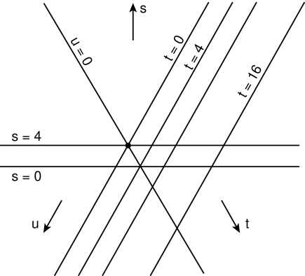
Figure 1: Mandelstam diagram

We assume Mandelstam representation where the scattering amplitude is

$$\frac{1}{\pi^{2}}\,\int\int\,\frac{ds^{\prime}dt^{\prime}\rho(s^{\prime},t^{\prime})}{(s^{\prime}-s)(t^{\prime}-t)}+{\rm circular\,permutations\,on}\,s,t,u$$ (2)

$$+{\rm subtractions}$$

with $s+t+u=4$.

In fact we use a much smaller domain of analyticity than Mandelstam (for a method of construction of such domains, see for instance Ref. [3]). However, the domain obtained from axiomatic field theory and unitarity [3] is not sufficient.

We assume $F(s,t)\sim sf(t)$, but from crossing in the $s\rightleftharpoons u$ variable we must have

$$F(s,t)\sim i\;s\,f(t),$$ (3)

$f(t)$ real for $t\leq 0$, so that the asymptotic absorptive part is just $sf(t)$, where $f(t)$ must have a cut from $t=4$ to $\infty$, and the double spectral function is given by

$$\rho(s,t)\simeq s\,Im\,f(t).$$ (4)

Now Gribov uses elastic unitarity in the elastic strip of the $t$ channel which, originally, reads:

$$A_{t}(t,z_{t})=\int K(t,z_{t},z^{\prime}_{t},z^{\prime\prime}_{t})F(t,z^{\prime}_{t})\,F(t,z^{\prime\prime}_{t})\;dz^{\prime}_{t}dz^{\prime\prime}_{t}$$ (5)

where $z_{t}=1+2s/(t-4)$ is the cosine of the scattering angle in the $t$ channel. Equation (5) is just a fancy way to write a spherical convolution of $F$ and $F^{*}$. $K$ is a known kernel, the square root of a polynomial whose support is entirely in the physical region.

Because of Mandelstam representation, $A_{t}(t,z_{t}),F(t,z_{t}),F^{*}(t,z^{*}_{t})$ are all analytic in a cut plane in $z_{t}$, with cuts at $z_{t}=\pm(1+8/(t-4))$, and Equation (5), as shown by Mandelstam, can be continued on the cuts, and transformed into a relation connecting the discontinuities of $A_{t},F$ and $F^{*}$:

$$\rho(s,t)=\int\hat{K}(t,s,s_{1},s_{2})A_{s}(s_{1},t)A^{*}_{s}(s_{2},t)ds_{1}ds_{2}$$ (6)

$\hat{K}$ is again a completely known expression with a finite support in $s_{1},s_{2}$ for given $s$ and $t$.

When $s\to\infty$, the domain of integration grows in such a way that the maximum of $s_{1}$ and $s_{2}$ also tends to infinity, and it is not difficult to convince oneself that if $A_{s}\sim s\,f(t)$, the dominating region of the integral is such that both $s_{1}$ and $s_{2}\to\infty$. It is not difficult to see that the right-hand side of Eq. (6) behaves like

$$|f(t)|^{2}\,s\,\log\,s$$ (7)

while the left-hand side is obviously

$$\rho=s\,Im\,f(t)$$ (8)

This is the Gribov contradiction, which occurs also for $F\sim s/\log\,s$. Only if $F\sim s/(log\,s)^{1+\epsilon}$ is the contradiction removed. This was the way out that Gribov proposed, corresponding to a total cross-section going to zero, but Nature did not make this choice. As we have known since 1972, cross-sections are rising [4] and might go to infinity at infinite energy.

Another way of looking at the Gribov phenomena is to use the complex angular momentum plane. In this language, the Gribov theorem says that elastic unitarity in the $t$ channel forbids a “fixed pole” at $J=1$. It is slightly more general in the sense that it is clearly insufficient to take an amplitude

$$i\,s\,f(t)+g(t)s^{\alpha(t)}$$ (9)

with $\alpha(t)<1$ for $t\leq 0$ and $Re\alpha(t)>1$ for $t>4m^{2}_{\pi}$ to “turn” the Gribov Theorem. In this version one clearly sees that the Donnachie-Landshoff odderon[5], $s\,t^{-4}$, is also, strictly speaking, forbidden unless there is an insurmountable natural boundary in the complex angular momentum plane.

One of the reasons for our renewed interest in the Gribov theorem is that there is another problem concerning high-energy cross-sections. As we said, we know that they are rising, possibly to infinity, possibly saturating qualitatively[4] the Froissart-Martin bound[6]

$$\sigma_{t}<C(\log\,s)^{2}$$ (10)

The question is to know if this bound can be saturated if one takes into account unitarity constraints. The simplest unitarity constraint is:

$$Im\,f_{\ell}(s)\geq\frac{2k}{\sqrt{s}}\,\left|f_{\ell}(s)\right|^{2}$$ (11)

when $f_{\ell}(s)$ is a partial wave amplitude. It is valid at all energies.

Joachim Kupsch has been able to show the existence of amplitudes which satisfy Mandelstam representation and the general unitarity constraint (11), and saturate the bound (10) [7]. This was a formidable achievement, taking into account all the restrictions that amplitudes saturating (10) must satisfy, in particular the so-called AKM conditions [8].

However, it is legitimate to ask oneself if the elastic unitarity condition in the elastic region

$$Im\,f_{\ell}(s)=\frac{2k}{\sqrt{s}}\,\left|k_{\ell}(s)\right|^{2},$$ (12)

which is so constraining in the Gribov case, might prevent the qualitative saturation of the Froissart bound. Turning the argument upside down, we may ask if the Gribov theorem survives if we require only (11) but not (12).

We want to show, and have almost succeeded in doing so, that there are explicit examples of amplitudes behaving like $s\,f(t)$ i.e., violating Gribov’s theorem, satisfying the general condition (11) at all energies. If this is so, all doubts are allowed concerning the other problem, the saturation of the Froissart bound because, while D. Atkinson succeeded in 1970 [9] to construct amplitudes satisfying (11) and (12) but with cross-sections decreasing faster than $(\log\,s)^{-2}$, nobody has succeeded in saturating the Froissart bound at the same time.

If it were to be shown one day that (12) prevents the qualitative saturation of the Froissart bound, it would be a major blow to many models such as the one of Bourrely-Cheng-Soffer-Walker-Wu[10], where $\sigma_{t}\sim(\log\,s)^{2}$ at extreme energies. I admit that the likelihood of this happening is very small, first of all because it requires somebody with great classical mathematical skill, who would tend naturally to use his abilities on a more fashionable subject. Nevertheless, we are allowed to raise the question.

2 A Candidate for Violating Gribov’s Theorem

We propose to take

$$F=C[F_{s}+F_{t}+F_{u}]$$ (13)

$$F_{s} = (4-\sqrt{4-t}\sqrt{4-u})\exp-2(4-s)^{1/4}$$

$$F_{t} = (4-\sqrt{4-u}\sqrt{4-s})\exp-2(4-t)^{1/4}$$

$$F_{u} = (4-\sqrt{4-t}\sqrt{4-s})\exp-2(4-u)^{1/4}$$ (14)

For $s\to\infty$, $t$ fixed, $F_{t}$ dominates and behaves like $i\,s\,\exp-2(4-t)^{1/4}$, which is what we want. We must now show that (11) is satisifed and, first of all, that all partial waves have a positive imaginary part. It is possible to show that in this channel $Im(F_{t}+F_{u})$ has positive partial wave amplitudes, because $Im(F_{t}+F_{u})$ can be expanded in powers of $\cos\theta_{s}$:

$$Im(F_{t}+F_{u})=\Sigma\,C_{n}(\cos\theta_{s})^{n},$$ (15)

and it can be shown that the $C_{n}$’s are positive.

Then, since

$$(\cos\theta)^{n}=\Sigma\,C_{\ell,n}\,P_{\ell}(\cos\theta)$$ (16)

with $C_{\ell,n}>0$, positivity of the partial waves follows. Another consequence from (15) and (16) is that the partial waves of $Im(F_{t}+F_{u})$ are decreasing. However, $ImF_{s}$ has oscillating signs, and though, globally, it is small in the $s$ channel, it must be proved that it is small partial wave by partial wave.

There are limiting cases where the behaviour is correct:

i) $\ell$ fixed, $k\to\infty$ and, in fact, also $k\to\infty$ and $\ell\to\infty$ with $\ell/k\to 0$, which allows $\ell\to\infty$ in some way. Then from the direct integration of $F$ with $P_{\ell}(\cos\theta_{s})$ one gets:

$$f_{\ell} \simeq \left(\frac{8}{s}+2i\right)\,\int^{0}_{-\infty}\,dt\,\exp\,-2(4-t)^{1/4}$$ (17)

$$\simeq \left(\frac{4}{s}+i\right)\,(15+14\sqrt{s})\,\exp\,-3\sqrt{2}$$

This shows that “unitarity” is satisfied just by adjusting $C$ in (13).

ii) $k$ fixed, $\ell\to\infty$ and more generally $\ell/k\to\infty$, $\ell\to\infty$. Then one has to use the Froissart-Gribov representation of the different contributions of the partial waves of the form

$$x_{\ell}=\int^{\infty}_{u}\,w(s,t)\,Q_{\ell}\left(1+\frac{t}{2k^{2}}\right)\,\frac{dt}{2k^{2}}$$ (18)

If

$$w\sim C(s)(t-4)^{\nu}$$ (19)

we get for $\ell\to\infty$, $\ell/k\to\infty$:

$$x_{\ell}\sim C(s)\left(\frac{2k\sqrt{2}}{\ell+1}\right)^{\nu+1}\,\Gamma(\nu+1)\,Q_{\ell}\left(1+\frac{2}{k^{2}}\right)$$ (20)

In this way it is trivial to see that the contribution from $Im(F_{u}+F_{t})$ dominates all the rest and that unitarity and positivity are satisfied.

iii) Finally, in the “scaling limit”

$$\frac{\ell+1}{k}=b,\,b\,{\rm fixed}\,k\to\infty$$ (21)

one can use the asymptotic expression for the $Q_{\ell}$’s valid for large $\ell$, uniform in $\phi$:

$$Q_{\ell}(\cosh\phi)\simeq\sqrt{\frac{\phi}{\sinh\phi}}\,K_{0}\left((\ell+1/2)\phi\right)$$ (22)

The RHS contribution to $ImF^{t}_{\ell}$ becomes:

$$\frac{1}{2k^{2}}\,\int\,dt\,K_{0}(b\sqrt{t})\,\sin\sqrt{2}(t-4)^{1/4}\,\exp-\sqrt{2}(t-4)^{1/4},$$ (23)

and is necessarily positive, because of the positivity properties of $Im(F_{t}+F_{u})$, and necessarily dominates all the other terms, the real parts and the contribution from $ImF_{s}$ which decrease exponentially with $s$.

iv) Unitarity of the $\ell=0$ partial wave can be checked by hand. There, in the expression $(4-\sqrt{4-t}\sqrt{4-u})$, the cancellation at $s=4$ is essential.

We conclude that it is only necessary to check unitarity in a finite region of the $\ell,k$ domain. First we did this numerically. Tests, at selected energies where unitarity seems endangered by the negative signs of the partial wave expansion of $ImF_{s}$, indicate that provided one divides the amplitude by a factor 2.1, there does not seem to be any violation. These tests are presented in Table 1.

However, we believe that by using old and new properties of the $Q_{\ell}$’s, for instance

$${\rm-old:}\,Q_{L}(z)/Q_{\ell}(z),{\rm decreases\,with}\;z\;{\rm for}\,L>\ell$$ (24)

$${\rm-new:}\,Q_{M-1}\left(1+\frac{t}{2k^{2}}\right)/Q_{m-1}\,\left(1+(\frac{M}{m})^{2}\,\frac{t}{2k^{2}}\right)\,{\rm decreases\,with}\,t\,{\rm for}\,M>m$$ (25)

We can complete the proof analytically, except for the calculation of a small, finite number of integrals over a finite interval.

Let us illustrate by two examples how we use (24) and (25). One problem is to find a lower bound on

$$ImF^{\ell}_{t,RHC}=$$

$$\frac{1}{2k^{2}}\int\limits^{\infty}_{4}\,Q_{\ell}\left(1+\frac{t}{2k^{2}}\right)\,\sqrt{s-4}\sqrt{s+t}\,\sin\sqrt{2}(t-4)^{1/4}\,\exp-\sqrt{2}(t-4)^{1/4}\,dt.$$

With the change of variable $x=\sqrt{2}(t-4)^{1/4}$, the integral becomes

$$\int^{\infty}_{0}\,W(x,s)\,sin\,x\,dx.$$

It is easy to prove that for $x>2\pi$, $W(x,s)$ is decreasing in $x$. Hence

$$\int^{\infty}_{2\pi}\,W(x,s)\,\sin\,x\,dx>0.$$

So

$$ImF^{\ell}_{t,RHC}>g_{\ell}(s)=$$

$$\frac{1}{2k^{2}}\int\limits_{4}^{4(1+\pi^{4})}\!\!\!\!\!\!Q_{\ell}\left(1+\frac{t}{2k^{2}}\right)\,\sqrt{s-4}\sqrt{s+t}\,\sin\sqrt{2}(t-4)^{1/4}\,\exp-\sqrt{2}(t-4)^{1/4}\,dt.$$

In $g_{\ell}$ the integrant has a single change of sign at $t_{0}=4+\frac{\pi^{4}}{4}$. If $g_{\ell_{0}}(s_{0})>0$, it follows from (24) that

$$g_{\ell}(s_{0})>g_{\ell_{0}}(s_{0})\,\frac{Q_{\ell_{0}}\left(1+\frac{t_{0}}{2k^{2}}\right)}{Q_{\ell}\left(1+\frac{t}{2k^{2}}\right)}$$

if $\ell>\ell_{0}$, and hence we get a lower bound on $Imf^{\ell}_{t,RHC}(s_{0})$ for $\ell>\ell_{0}$, but we can also change at the same time $\ell$ and $s$ and use (25) to get a lower bound for

$$\frac{\ell+1}{2k^{2}}=\frac{\ell_{0}+1}{2k^{2}_{0}},\,\ell>\ell_{0}.$$

Finally, we can also use the fact that $Im\left(f^{\ell}_{t}+f^{\ell}_{u}\right)$ is decreasing with $\ell$ to get lower bounds for smaller $\ell$’s.

Everybody will understand that this is a rather delicate book-keeping, but with enough patience, we will succeed.

3 Conclusions

If you believe that our example, after “renormalization”, satisfies the general unitarity condition (11), you conclude that the proof of Gribov’s theorem holds only if we impose elastic unitarity (12) in the elastic region. Incidentally, a kind of universality postulate is tacitly made by everybody, because everybody believes that the Gribov theorem applies to $pp$ scattering, while technically there are problems with the unphysical region in the $t$ channel which would disappear only if $m_{p}<1.5m_{\pi}$.

It is therefore legitimate to ask oneself what happens in another situation, the qualitative saturation of the Froissart bound, where the examples saturating this bound only satisfy condition (11) but not elastic unitarity. Would elastic unitarity make the saturation of the bound impossible?

My own prejudice is that this will not happen, but there is absolutely no proof of that. As pointed out by S.M. Roy, [11] it could be that elastic unitarity leads to a quantitative improvement of the Froissart bound, i.e., replacing the factor $\pi/m^{2}_{\pi}$, which appears in the Lukaszuk-Martin [12] version:

$$\sigma_{t}<\frac{\pi}{m_{\pi^{2}}}\,(\log s)^{2},$$

by something much smaller. In any case, we believe that these questions are worth investigating.

4 Acknowledgements

One of us (A.M.) would like to thank J. Kupsch and S.M. Roy for very stimulating discussions, and the Indo-French Centre for the Promotion of Advanced Research (IFCPAR) for support.

Table 1: Numerical tests of unitarity of (13), with $C=1$

$s$	$\ell$	$Ref_{\ell}$	$Imf_{\ell}$	$\sqrt{s}/2k\;Imf_{\ell}/|f_{\ell}|^{2}$
4.0001	0	0.473	0.00236	2.1
	2	4.1 $\times 10^{-11}$	5.1 $\times 10^{-12}$	6 $\times 10^{11}$
4.01	0	0.108	0.0040	2.19
	2	7 $\times 10^{-6}$	1.19 $\times 10^{-7}$	4 $\times 10^{5}$
	4	8.5 $\times 10^{-11}$	9.6 $\times 10^{-11}$	3.7 $\times 10^{10}$
50	0	0.53	1.45	0.63
	2	0.037	1.19	0.84
	4	0.0081	0.64	1.56
70	0	0.40	1.71	0.57
Chosen	2	-0.009	0.294	3.5
so that	4	0.002	0.0736	14
$Imf^{s}_{\ell}<0$	6	0.0008	0.0193	53
for $\ell>0$	8	0.00025	0.0054	190
3500	0	0.0055	2.06	0.49
	2	0.0017	1.82	0.54
	4	0.0017	1.51	0.66
idem	6	0.0014	1.21	0.82
	8	0.0011	0.96	1.04
	10	0.0009	0.76	1.32
	12	0.0007	0.60	1.67
	14	0.0005	0.477	2.1
	16	0.0004	0.380	2.62
	18	0.0003	0.305	3.3
	20	0.0003	0.245	4.1
24000	0	0.0003	2.05	0.49
	2	0.0003	2.01	0.49
	4	0.0003	1.94	0.51
	6	0.0003	1.84	0.54
	8	0.0003	1.72	0.58
	10	0.0003	1.60	0.63
	12	0.0002	1.47	0.68
	14	0.0002	1.35	0.74
Idem	16	0.0002	1.24	0.80
	18	0.0002	1.13	0.88
	20	0.0002	1.04	0.96
	22	0.0002	0.95	1.05
	24	0.0001	0.81	1.15
	26	0.0001	0.79	1.26
	28	0.0001	0.72	1.37
	30	0.0001	0.66	1.50
	32	0.0001	0.61	1.65
	34	0.0001	0.56	1.80
	36	0.0001	0.51	1.97
	38	0.0001	0.47	2.15
	40	0.0001	0.43	2.34
$\infty$	Any finite	0	(15 + 14 $\sqrt{2})\times$	0.486187
	$\ell$		$\exp-2\sqrt{2}$
			$\simeq 2.05602$

References

References

- [1] V.N. Gribov, Proceedings of the 1960 Annual International Conference on High-Energy Physics at Rochester, eds. E.C.G. Sudarshan, J.H. Tinlot and A.C. Melissos (University of Rochester 1960), p. 340.
- [2] The papers by Regge on Regge poles in potential scattering did exist, but the application to high-energy scattering was not yet fashionable.
- [3] A.Martin, Proceedings of the 1967 International Conference on Particles and Fields, eds. C.R. Hagen, G. Guralnik and V.A. Mathur (John Wiley and Sons, 1967), P. 252.
- [4] See, for instance, G. Matthiae, Rep. Prog. Phys. 57 (1994) 743.
- [5] A. Donnachie and P.V. Landshoff, Phys. Lett. B296 (1992) 227.
-
[6]
M. Froissart, Phys. Rev. 123 (1961) 1053;
A. Martin, Nuovo Cimento 42 (1966) 930. - [7] J. Kupsch, Nuovo Cimento 71A (1982) 85.
- [8] G. Auberson, T. Kinoshita and A. Martin, Phys. Rev. D3 (1971) 3185.
- [9] D. Atkinson, Nucl. Phys. B23 (1970) 397.
-
[10]
It is impossible to quote all references. We shall give three of them:
H. Cheng and T.T. Wu, Phys. Rev. Lett. 24 (1970) 1456;
H. Cheng, J.K. Walker and T. Tu, Phys. Lett.B44 (1973) 283;
C. Bourrely, J. Soffer and T.T. Wu, Nucl. Phys.B247 (1984) 15. - [11] S.M. Roy, private communication.
- [12] L. Lukaszuk and A. Martin, Nuovo Cimento 52A (1967) 122, Appendix E.