Hybrid Inflation and Baryogenesis at the TeV Scale

Abstract

We consider the construction of inverted hybrid inflation models in which the vacuum energy during inflation is at the TeV scale, and the inflaton couples to the Higgs field. Such models are of interest in the context of some recently proposed models of electroweak baryogenesis. We demonstrate how constraints on these models arise from quantum corrections, and how self-consistent examples may be constructed, albeit at the expense of fine-tuning. We discuss two possible ways in which the baryon asymmetry of the universe may be produced in these models. One of them is based on preheating and a consequent non-thermal electroweak symmetry restoration and the other on the formation of Higgs winding configurations by the Kibble mechanism at the end of inflation.

SUSX-TH/01-014, DAMTP-2001-18, SU-GP-01/2-3

I Introduction

There is overwhelming observational evidence (for recent reviews see, e.g., [1, 2, 3]) that the universe has a non-zero baryon density, quantified by

$$\frac{n_{B}}{s}\sim 10^{-10}\ ,$$ (1)

where $n_{B}$ is the baryon number density in the universe, and $s$ is the entropy density. Because a period of cosmological inflation [4, 5, 6] would have diluted away any baryons, this asymmetry must have been generated afterwards. One attractive possibility is that baryogenesis proceeds through anomalous electroweak processes occurring during the departure from equilibrium provided by the electroweak phase transition [7]. However, the transition must be strongly first order for electroweak sphaleron processes not to wash away the baryon asymmetry immediately after it is generated, and lattice Monte Carlo simulations have shown that this is not the case in the minimal standard model [8].

As an alternative to the above standard picture of electroweak baryogenesis, it has recently been suggested [9, 10] that the washout problem could be avoided if inflation ends at the electroweak scale, with the inflaton strongly coupled to the Higgs field. Preheating [11, 12], i.e., parametric resonance between the Higgs field and the inflaton, would lead to a non-equilibrium state in which the baryon asymmetry could be generated, and a low enough reheat temperature would guarantee that once the system has thermalized, sphaleron processes are too rare to wash it out. This idea has the attractive feature that it may predict new phenomena, testable in collider experiments, and thus provide a hope of a direct probe into the physics of the early universe.

Inflation model-building is however beset with difficulties, which become more severe as the inflation scale is decreased [13]. One problem is the difficulty in arranging the necessary initial conditions for inflation to begin [14, 15, 16, 17]. Another problem is to understand the extreme flatness of the potential, which requires that every tree-level and every loop-correction term in the potential be small unless there are cancellations between them. Turning to the case at hand, the most obvious way of achieving inflation with the inflaton strongly coupled to the Higgs field is to invoke the usual hybrid inflation model, in which the inflaton is rolling towards the origin. This paradigm, adopted so far [9, 10], is unfortunately spoiled by the loop correction [18]; its strong logarithmic variation prevents inflation, and cannot be cancelled by a reasonable number of tree-level terms. In this paper, we consider the alternative paradigm of inverted hybrid inflation, where the field is rolling away from the origin. In contrast with the usual case, the loop correction can now be cancelled accurately by a suitable choice of just the renormalizable tree–level terms, leading to a viable, albeit fine-tuned, model which can give successful baryogenesis.

The outline of the paper is as follows. In Section II, we discuss two different ways that baryon asymmetry can be generated. One of these is the scenario put forward in Refs. [9, 10], involving resonant production of sphalerons and Higgs winding configurations during preheating, and the other is based on the Kibble mechanism [19] and is a variant of the mechanism discussed in Refs. [20, 21]. In Section III, we recall the loop correction problem encountered with ordinary hybrid inflation, and in Section IV, we see how it can be avoided by inverted hybrid inflation if the mass and quartic self-coupling are fine-tuned to cancel the loop correction. In Section V, we determine the region of the parameter space in which our model satisfies the constraints arising from inflation and baryogenesis. Finally, we summarize the essential results of this paper and offer some comments on the role of low-scale inflation models.

II Baryogenesis after TeV-Scale Inflation

In the electroweak theory, baryon number is linked to the Chern-Simons number of the SU(2) gauge field

$$N_{\rm CS}={g^{2}\over 32\pi^{2}}\int_{0}^{t}dt\int d^{3}x\epsilon^{\mu\nu\rho\sigma}{\rm Tr}F_{\mu\nu}F_{\rho\sigma}$$ (2)

by a quantum anomaly [22],

$$\Delta B=3\Delta N_{\rm CS}.$$ (3)

In order to generate the baryon asymmetry, it is therefore necessary that the dynamics of the system leads to a non-zero Chern-Simons number.

The dynamics of the Chern-Simons number is linked to the dynamics of the Higgs field via the Higgs winding number

$$N_{H}=\frac{1}{24\pi^{2}}\int d^{3}x\,\epsilon^{ijk}\hbox{Tr}[U^{\dagger}\partial_{i}UU^{\dagger}\partial_{j}UU^{\dagger}\partial_{k}U].$$ (4)

In this parameterization, the $SU(2)$ Higgs field $\Phi$ has been expressed as $\Phi=({\rho}/{\sqrt{2}})U$, where $\rho^{2}=2\left(\varphi_{1}^{*}\varphi_{1}+\varphi_{2}^{*}\varphi_{2}\right)={\rm Tr}\Phi^{\dagger}\Phi$, and $U$ is an $SU(2)$-valued matrix that is uniquely defined anywhere $\rho$ is nonzero. In the broken phase we have in practice $N_{\rm CS}=N_{H}$, and thus any difference in the two numbers must disappear when the system thermalizes. This may either happen by changing the Chern-Simons number, which would lead to baryon production [20, 21], or by changing the Higgs winding, in which case no baryons are produced. CP-violation affects the balance between these two ways, and leads to an asymmetry in the final baryon number (see [23] for a detailed discussion of the dynamics of winding configurations).

A Baryogenesis from Preheating

One possibility for baryon production arises from reheating after cosmological inflation. Careful, non-perturbative studies [24, 25] of the inflaton dynamics have demonstrated that there may be a period of parametric resonance, prior to the usual scenario of energy transfer from the inflaton to other fields. This phenomenon is characterized by large amplitude, non-thermal excitations in both the inflaton and coupled fields, and has become known as preheating [11, 12].

In the models we consider in this paper, the inflaton is directly coupled to the standard model Higgs field. Therefore, if preheating occurs, we expect long-wavelength excitations of standard model fields to be resonantly produced. This may lead to a non-thermal restoration of the SU(2) symmetry [26, 27, 28], and to the production of a population of winding configurations [9] and a non-zero Chern-Simons number [10] even though the reheat temperature after inflation is never above the electroweak scale, and even though the electroweak symmetry remains broken after the end of inflation. Because of the non-perturbative nature of this mechanism, it is very difficult to derive reliable analytical estimates for the baryon asymmetry, and one has to resort to numerical simulations [29].

B Baryogenesis from the Kibble Mechanism

The mechanism of the previous section; preheating and a subsequent non-thermal symmetry restoration, needs an initial energy density that is much higher than the Higgs potential barrier. However, if the energy density is lower, there is another way the baryon asymmetry can be generated. This is based on the instability of the Higgs field (i.e., tachyonic preheating [30, 31]), which leads to formation of topological “defects” by the Kibble mechanism [19] when the SU(2) symmetry breaks.

In hybrid inflationary models, the Higgs field vanishes during inflation, and the electroweak symmetry is therefore unbroken. At the end of inflation, the Higgs field rolls to its true vacuum [30, 31]. The Kibble mechanism ensures that Higgs winding configurations will form, and CP violation inherent in many extensions of the standard model ensures that net baryon production results. Because the universe is cold after the inflation, the phase transition takes place at zero temperature. This means that there are no sphaleron processes that would wash out the baryon asymmetry, and consequently no need for a first-order phase transition. Of course, the universe eventually reheats to the temperature $T_{\rm rh}$, but if this is low enough so that the electroweak symmetry is strongly broken, the baryon asymmetry is safe.

The baryon number generated in this scenario can be estimated by finding the shortest wavelength that falls out of equilibrium [32]. When the inflaton field $\sigma$ rolls toward its minimum, the effective mass squared of the Higgs field $m^{2}(\sigma)$ changes, and at $\sigma=\sigma_{c}$ it changes sign. Assuming that a Fourier mode with momentum $k$ is in equilibrium, its frequency is given by

$$\omega(k)^{2}=k^{2}+m^{2}(\sigma).$$ (5)

If the equation

$$\left|\frac{d\omega(k)}{dt}\right|\mathrel{\raise 1.29167pt\hbox{$>$}\mkern-14.0mu\lower 2.58334pt\hbox{$\sim$}}\omega(k)^{2}$$ (6)

is satisfied, the mode behaves non-adiabatically, i.e., it evolves so slowly that it does not have time to adjust to the change of its effective mass. Consequently, the mode falls out of equilibrium. In general, there is a critical momentum $k_{\rm max}$ such that this happens for $k\leq k_{\rm max}$. The maximum correlation length reached during the transition is given by $\xi_{\rm max}=k_{\rm max}^{-1}$.

When $m^{2}(\sigma)$ becomes negative at $\sigma_{c}$, the Higgs field acquires a non-zero expectation value, but its direction can only be correlated at distances less than $\xi_{\rm max}$. This leads to domains of radius $\xi_{\rm max}$, inside each of which the Higgs field is roughly constant, and when the field is interpolated between these domains, it typically acquires a non-zero winding number. The resulting number density of these winding configurations is determined by the domain size,

$$n_{\rm configs}\sim\xi_{\rm max}^{-3}\sim k_{\rm max}^{3},$$ (7)

and a rough estimate indicates that this density must be higher than $0.001m_{H}^{3}$ for sufficient baryogenesis [9].

The above analysis ignores the gauge field, which plays an important role in defect formation in the high-temperature case [33]. The reason why this is justified here is that the effect of the gauge field is proportional to the temperature, and in our case, the symmetry breaking takes place at zero temperature.

III Constraints on Hybrid Inflation Models

A Basics

In order to analyse the viability of different models of TeV-scale inflation, let us first summarize the basics of inflation model building, as given in say [13]. We write the reduced Planck mass as $M_{\rm P}\equiv(8\pi G)^{-1/2}=2.4\times 10^{18}\,\mbox{GeV}$, and the Hubble parameter as $H$. Further, an overdot denotes differentiation with respect to time and the prime differentiation with respect to the inflaton field $\sigma$.

We will be interested in the slow-roll paradigm of inflation in which the field equation for the inflaton $\sigma$

$$\ddot{\sigma}+3H\dot{\sigma}+V^{\prime}=0\ ,$$ (8)

is replaced by the slow-roll condition

$$3H\dot{\sigma}\simeq-V^{\prime}\ .$$ (9)

We also require

$$V\simeq\rho\simeq 3M_{\rm P}^{2}H^{2}\ ,$$ (10)

with $\rho$ the energy density, be almost constant on the Hubble timescale. The latter condition requires one flatness condition

$$\epsilon\ll 1\,,$$ (11)

and differentiating the slow-roll condition requires a second flatness condition

$$|\eta|\ll 1\,,$$ (12)

where

$$\epsilon \equiv \frac{1}{2}M_{\rm P}^{2}\left(\frac{V^{\prime}}{V}\right)^{2}\,,$$ (13)

$$\eta \equiv M_{\rm P}^{2}\frac{V^{\prime\prime}}{V}\,.$$ (14)

$N$ $e$-folds before the end of slow-roll inflation, the field value $\sigma_{N}$ is given by

$$N=\frac{1}{M_{\rm P}^{2}}\int^{\sigma_{N}}_{\sigma_{\rm end}}\frac{V}{V^{\prime}}d\sigma\,,$$ (15)

where $\sigma_{\rm end}$ marks the end of slow-roll inflation.

If the inflaton field fluctuation is responsible for structure in the Universe, the COBE measurement of the cosmic microwave background anisotropy requires

$$\frac{V(\sigma_{\rm COBE})^{3/2}}{M_{\rm P}^{3}V^{\prime}(\sigma_{\rm COBE})}=5.3\times 10^{-4}\,.$$ (16)

This equation applies at the epoch when the distance scale explored by COBE (say $H_{0}^{-1}/10$) leaves the horizon, some number $N_{\rm COBE}<60$ $e$-folds before the end of slow-roll inflation.

B Ordinary hybrid inflation

In Refs. [9, 10], baryogenesis was discussed in the context of ordinary hybrid inflation. In this model, the tree-level potential is [34]

$$V(\sigma,\phi)=V_{0}+\Delta V(\sigma)-\frac{1}{2}|m^{2}|\phi^{2}+\frac{1}{2}{g^{2}}\phi^{2}\sigma^{2}+\frac{1}{4}\lambda\phi^{4}\,,$$ (17)

where, in the simplest model,

$$\Delta V(\sigma)=\frac{1}{2}m_{\sigma}^{2}\sigma^{2}\,.$$ (18)

Inflation takes place in the regime $\sigma^{2}>\sigma_{\rm c}^{2}$, where

$$\sigma_{\rm c}\equiv\frac{|m|}{g}\,.$$ (19)

In this regime, $\phi$ vanishes and the inflaton potential is

$$V=V_{0}+\Delta V(\sigma)\ ,$$ (20)

where the constant term $V_{0}$ is assumed to dominate during inflation [34, 35].

The specific implementation proposed in [9, 10] involved the tree-level hybrid inflation model using the Higgs as the non-inflaton field. This same paradigm was suggested later [36] (without specifically invoking the Higgs field) as a model of inflation with quantum gravity at the TeV scale. Unfortunately both of these proposals are spoiled by the loop correction [18].

To see how this comes about, let us first pursue the model ignoring the loop correction. The last term of Eq. (17) serves only to determine the vacuum expectation value (VEV) of $\phi$, achieved when $\sigma$ falls below $\sigma_{\rm c}$. Demanding that $V$ vanish in the vacuum, so that the cosmological constant is zero after inflation, implies that the VEV is

$$\langle\phi\rangle\equiv v=2\frac{V_{0}^{1/2}}{|m|}\,,$$ (21)

and that

$$\lambda=\frac{4V_{0}}{v^{4}}=\frac{m^{4}}{4V_{0}}\,.$$ (22)

From Eq. (18),

$$\eta=\frac{m_{\sigma}^{2}M_{\rm P}^{2}}{V_{0}}\,.$$ (23)

It will be useful also to define

$$\eta_{\phi}\equiv\frac{|m^{2}|M_{\rm P}^{2}}{V_{0}}=\frac{4M_{\rm P}^{2}}{v^{2}}\,.$$ (24)

A prompt end to inflation at $\sigma_{\rm c}$ requires

$$\eta_{\phi}\mathrel{\raise 1.29167pt\hbox{$>$}\mkern-14.0mu\lower 2.58334pt\hbox{$\sim$}}1\,,$$ (25)

which is well satisfied. Now, the value of the field $\sigma$ when COBE scales leave the horizon is

$$\sigma_{\rm COBE}^{2}=e^{2\eta N_{\rm COBE}}\sigma_{\rm c}^{2}\simeq\sigma_{\rm c}^{2}\,,$$ (26)

where the final equality is good for an order of magnitude estimate, but needs to be checked for consistency in any particular example. Using (26), the COBE normalization is

$${g^{2}} = 2.8\times 10^{-7}e^{2\eta N_{\rm COBE}}\eta^{2}\eta_{\phi}$$ (27)

$$\simeq 3\times 10^{-7}\eta^{2}\eta_{\phi}\,.$$ (28)

To identify $\phi$ with the Higgs field we need roughly $m\sim$ TeV and $\lambda\sim 1$ (corresponding to $V_{0}^{1/4}\sim v\approx 250$ GeV) and for baryogenesis to work we need a strong coupling to the Higgs field, $g\sim 1$. The COBE normalization then requires $m_{\sigma}\sim 10^{-10}\,\mbox{eV}$, which corresponds to $\eta\simeq 10^{-15}$, justifying the final equality in Eq. (26). Because $\eta$ is so small, $\sigma$ is practically equal to the critical value $\sigma_{\rm c}$ while scales of interest are leaving the horizon. On the other hand, it seems reasonable to require that inflation occurs over some reasonable range of $\sigma$, since otherwise one would have to explain how $\sigma$ arrived at precisely the value $\sigma_{\rm c}$.

The small value of $m_{\sigma}$ means that even if the loop correction did not spoil the model, the energy density at the end of inflation would be too low for the scenarios discussed in Section II. Because of the slow-roll condition (9), the kinetic energy is negligibly small,

$$\frac{1}{2}\dot{\sigma}^{2}=\frac{M_{p}^{2}V^{\prime 2}}{6V}\sim\frac{M_{p}^{2}m_{\sigma}^{4}}{m_{H}^{2}}\mathrel{\raise 1.29167pt\hbox{$<$}\mkern-14.0mu\lower 2.58334pt\hbox{$\sim$}}(0.01~{}{\rm eV})^{4}.$$ (29)

The energy density consists therefore only of the potential energy, which at $\sigma=\sigma_{c}$ is $V(\sigma_{c})=V_{0}+\frac{1}{2}m_{\sigma}^{2}\sigma_{c}^{2}\approx V_{0}$. Because $V_{0}$ is the height of the Higgs barrier, the energy density must be much higher than this for symmetry restoration as discussed in Section II A to be possible. The low kinetic energy also means that the Kibble mechanism discussed in Section II B cannot lead to significant baryogenesis either.

Now consider the loop correction, coming from the Higgs field. Part of this correction just renormalizes the mass and quartic self-coupling of the inflaton field. If there is no supersymmetry (SUSY), one has to take the view that the renormalized couplings are set to desired values, making this part of the loop correction insignificant. If, on the other hand, there is supersymmetry, this part of the loop correction vanishes (in the global supersymmetric limit, with soft or spontaneous SUSY breaking, and after the Higgsino and the other Higgs field have been included). The other, logarithmic, part of the loop correction is more problematic. This contribution is

$$\Delta V_{\rm loop}(\sigma)=\frac{1}{64\pi^{2}}\left(m^{4}(\sigma){\rm ln}\frac{m^{2}(\sigma)}{Q^{2}}\right)\,,$$ (30)

where

$$m^{2}(\sigma)\equiv\left({g^{2}}\sigma^{2}-|m^{2}|\right)={g^{2}}(\sigma^{2}-\sigma_{\rm c}^{2})\,.$$ (31)

The quantity $Q$ is the renormalization scale at which the parameters of the tree-level potential should be evaluated. Its choice is arbitrary, and if all loop corrections were included, the total potential would be independent of $Q$ by virtue of the Renormalization Group Equations (RGEs). In any application of quantum field theory, one should choose $Q$ so that the total 1-loop correction is small, hopefully justifying the neglect of the multi-loop correction.

Unless $\sigma$ is extremely close to $\sigma_{\rm c}$, the loop correction and its derivatives are roughly estimated by setting $\sigma_{\rm c}=0$, giving

$$\Delta V_{\rm loop} = \frac{g^{4}}{64\pi^{2}}\sigma^{4}\ln\frac{g^{2}\sigma^{2}}{Q^{2}},$$ (32)

$$\Delta V_{\rm loop}^{\prime} = \frac{g^{4}}{32\pi^{2}}\sigma^{3}\left(2\ln\frac{g^{2}\sigma^{2}}{Q^{2}}+1\right),$$ (33)

$$\Delta V_{\rm loop}^{\prime\prime} = \frac{g^{4}}{32\pi^{2}}\sigma^{2}\left(6\ln\frac{g^{2}\sigma^{2}}{Q^{2}}+7\right).$$ (34)

Because of the logarithmic variation, the loop correction cannot be cancelled to high accuracy over a reasonable range of $\sigma$, by a tree-level contribution containing a reasonable number of terms. The flatness conditions $\epsilon\ll 1$ and $\eta\ll 1$ therefore both require

$$g\ll\frac{v}{M_{\rm P}}\,.$$ (35)

(One of these can be avoided by a choice of $Q$, but not both.) This constraint precludes a VEV $v$ at the TeV scale, except for an unfeasibly small value of $g$. It holds independently of the form of the tree-level contribution. Taking the simplest form Eq. (18), requiring that the COBE normalization is not upset by the loop correction gives an additional constraint [18]

$$v^{4}\sigma_{\rm COBE}\mathrel{\raise 1.29167pt\hbox{$>$}\mkern-14.0mu\lower 2.58334pt\hbox{$\sim$}}\left(10^{9}\,\mbox{GeV}\right)^{5}\left(\frac{V_{0}^{1/4}}{1\,\mbox{MeV}}\right)^{2}\,.$$ (36)

This precludes, by many orders of magnitude, hybrid inflation with $\sigma_{\rm COBE}$, $v$ and $V_{0}^{1/4}$ at the TeV scale.

As we noted earlier, with TeV–scale inflation, length scales corresponding to our observable Universe, actually leave the horizon when $\sigma$ is very close to $\sigma_{\rm c}$. In principle, one could therefore avoid the above constraints by starting the inflation very close to $\sigma_{c}$. In that regime the loop correction is very suppressed, and so is its first derivative making $\epsilon$ very small. Although the second derivative is not suppressed in general, it can be suppressed at any single point by a suitable choice of the renormalization scale $Q$. However, the third derivative $\Delta V_{\rm loop}^{\prime\prime\prime}$ will not be suppressed at the same point, and near $\sigma_{c}$ it is roughly

$$\Delta V_{\rm loop}^{\prime\prime\prime}\sim\frac{g^{4}\sigma_{c}^{2}}{\sigma-\sigma_{c}}.$$ (37)

Therefore, even if we tune $Q$ in such a way that the the slow-roll condition (12) is satisfied at $\sigma$, the length of the range inside which it remains satisfied is of order

$$\Delta\sigma\sim\frac{V_{0}(\sigma-\sigma_{c})}{g^{2}|m^{2}|M_{p}^{2}}\sim\frac{v^{2}}{M_{p}^{2}}(\sigma-\sigma_{c})\approx 10^{-32}(\sigma-\sigma_{c}).$$ (38)

This is far too short to produce any inflation at all in practice, because Eq. (15) implies that $N\approx\Delta\sigma/\eta\sigma\sim 10^{-17}(\sigma-\sigma_{c})/\sigma$. We conclude that the hybrid inflation paradigm is unviable at the TeV scale, and turn now to an alternative.

IV Inverted hybrid inflation

Given the concerns discussed in the previous section, we shall turn from ordinary hybrid inflation, in which the inflaton rolls towards the origin, and consider instead the case of inverted hybrid inflation [37, 38, 39] where it rolls away from the origin, and inflation takes place at small $\sigma$. This is achieved by giving $\Delta V$ a negative slope, making the coupling between $\phi$ and $\sigma$ negative, and making $m^{2}$ positive.

The effective potential we shall consider is

$$V(\phi,\sigma)=V_{0}-{1\over p}\lambda_{p}\sigma^{p}+{1\over q}\kappa_{q}\sigma^{q}-{1\over 2}g^{2}\sigma^{2}\phi^{2}+{1\over 2}m^{2}\phi^{2}+{1\over 4}\lambda\phi^{4}\ ,$$ (39)

where all the parameters in the potential are positive semi-definite. To have a viable model we shall need to consider non-renormalizable terms $q>p>4$, corresponding to dimensionful parameters $\lambda_{p}$ and $\kappa_{q}$.

The tree-level mass term $m^{2}$ of the Higgs field is positive, and therefore the electroweak symmetry is restored during inflation, when $\sigma$ is small. When $\sigma$ reaches the critical value $\sigma_{c}=m/g$, the Higgs field becomes unstable and the symmetry gets broken. If we assume that the time scale of the dynamics of the Higgs field is much faster than that of the inflaton, we can calculate that at any value of $\sigma$, the Higgs field has the value

$$\phi^{2}=\phi_{\rm min}^{2}={g^{2}\sigma^{2}-m^{2}\over\lambda}\ .$$ (40)

Thus the effective potential for the inflaton $\sigma$ is

$$V_{\rm eff}(\sigma)=V_{0}-{m^{4}\over 4\lambda}+{1\over 2}\frac{g^{2}m^{2}}{\lambda}\sigma^{2}-\frac{g^{4}}{4\lambda}\sigma^{4}-{1\over p}\lambda_{p}\sigma^{p}+{1\over q}\kappa_{q}\sigma^{q}\ .$$ (41)

The loop correction is given by the same expression (30) as before. At $\sigma\gg\sigma_{c}$, it behaves as $\Delta V_{\rm loop}(\sigma)\sim\sigma^{4}\ln\sigma$, which is of lower order than the tree-level terms $\sigma^{p}$ and $\sigma^{q}$, and therefore we can ignore the loop correction when we study the dynamics after inflation. During inflation, $\sigma<\sigma_{c}$, so that,

$$m^{2}(\sigma)=m^{2}-g^{2}\sigma^{2}=g^{2}(\sigma_{\rm c}^{2}-\sigma^{2}).$$ (42)

An appropriate choice in this regime is $Q=m$, and with that choice the loop correction is a power series, equivalent to a tree-level contribution. At sufficiently small $\sigma$, the series converges rapidly and we need keep only the renormalizable terms (quadratic and quartic). In the language of effective field theory, we have obtained an effective field theory valid at $\sigma\ll m$ by integrating out the physics on the scale $m$. This is analogous to the way in which one might obtain the Standard Model by integrating out GUT physics on the scale $M_{\rm GUT}$.

In order to satisfy the slow-roll and COBE constraints, the potential must be very flat at small $\sigma$, where inflation takes place. As a result, at least the quadratic and quartic terms must be cancelled, by the tree-level terms of the original potential. Demanding a perfect cancellation, we arrive at the “renormalized” loop correction

$$\Delta V_{\rm loop}(\sigma)=\frac{1}{64\pi^{2}}\left[m^{4}(\sigma){\rm ln}\frac{m^{2}(\sigma)}{m^{2}}+g^{2}m^{2}\sigma^{2}-\frac{3}{2}g^{4}\sigma^{4}\right].$$ (43)

To achieve slow-roll inflation the inflaton mass-squared has to be much less than $V_{0}/M_{\rm P}^{2}\sim 10^{-30}m^{2}\sim(10^{-4}\,\mbox{eV})^{2}$, which means that the quadratic counter-term has to cancel the loop correction to an accuracy of $10^{-30}$. Also, the dimensionless coupling of the quartic term has to be $\mathrel{\raise 1.29167pt\hbox{$<$}\mkern-14.0mu\lower 2.58334pt\hbox{$\sim$}}10^{-15}$ to achieve the COBE normalization, and the quartic counter-term has to cancel the loop correction to this accuracy. These two extremely fine-tuned cancellations are the price we have to pay, for the not inconsiderable prize of inflation at the TeV scale with an unsuppressed coupling to the Higgs field leading to viable baryogenesis. From the effective field theory viewpoint, we have renormalized the parameters of the effective small-$\sigma$ potential, in an analogous way to that in which the parameters of the Standard Model effective theory are renormalized if it is obtained from a non-supersymmetric GUT theory.

The next term in the power series representing the loop correction is

$$\Delta V_{\rm loop}(\sigma)=-\frac{1}{192\pi^{2}}\frac{g^{6}\sigma^{6}}{m^{2}},$$ (44)

and we shall check that this does not spoil the COBE normalization.

Now, the effective potential (41) is minimized when

$$\kappa_{q}\sigma_{\rm min}^{q-2}-\lambda_{p}\sigma_{\rm min}^{p-2}-\frac{g^{4}}{\lambda}\sigma_{\rm min}^{2}+\frac{g^{2}m^{2}}{\lambda}=0\ .$$ (45)

Assuming that $g^{2}$ is small, the mass of the Higgs field in this minimum, which corresponds to the physical vacuum, is

$$m_{H}^{2}=2(g^{2}\sigma^{2}_{\rm min}-m^{2})\ .$$ (46)

Because $m_{H}^{2}$ is an observable quantity, and $\sigma_{\rm min}$ is not, it is useful to invert this relation and write

$$\sigma^{2}_{\rm min}=\frac{1}{g^{2}}\left(m^{2}+\frac{1}{2}m_{H}^{2}\right)\ .$$ (47)

By requiring $V(\sigma_{\rm min})=0$, i.e. that the cosmological constant be zero in the physical vacuum, and using (47), we may express $V_{0}$ in terms of the other parameters as

$$V_{0} = -\frac{m^{2}}{\lambda}\left(\frac{1}{2}-\frac{1}{q}\right)\left(m^{2}+\frac{1}{2}m_{H}^{2}\right)+\frac{1}{\lambda}\left(\frac{1}{4}-\frac{1}{q}\right)\left(m^{2}+\frac{1}{2}m_{H}^{2}\right)^{2}$$ (49)

$$+\frac{\lambda_{p}}{g^{p}}\left(\frac{1}{p}-\frac{1}{q}\right)\left(m^{2}+\frac{1}{2}m_{H}^{2}\right)^{p/2}+\frac{m^{4}}{4\lambda}\ .$$

For future convenience, let us introduce the dimensionless parameters

$$\alpha\equiv\frac{2m^{2}}{m_{H}^{2}},\qquad\beta\equiv\frac{\lambda\lambda_{p}}{m_{H}^{4}}\sigma_{\rm min}^{p}.$$ (50)

In terms of these parameters, the initial energy density Eq. (49) is

$$\rho_{\rm init}=V(\phi=0,\sigma=0)=V_{0}=\frac{m_{H}^{4}}{4\lambda}\left[\frac{1}{4}-\frac{\alpha+1}{q}+4\frac{q-p}{pq}\beta\right].$$ (51)

Using Eq. (45), we can also express $\kappa_{q}$ in terms of $m_{H}^{2}$ as

$$\kappa_{q} = g^{q}\left(m^{2}+\frac{1}{2}m_{H}^{2}\right)^{1-q/2}\left[\frac{m_{H}^{2}}{2\lambda}+\frac{\lambda_{p}}{g^{p}}\left(m^{2}+\frac{1}{2}m_{H}^{2}\right)^{p/2-1}\right]$$ (52)

$$= \frac{g^{q}m_{H}^{4-q}}{\lambda}\left[\frac{\alpha+1}{4}+\beta\right]\left(\frac{\alpha+1}{2}\right)^{-q/2}.$$ (53)

V Cosmological Constraints

Having defined the model, we now turn to the constraints imposed by the requirement of a successful cosmological evolution. In particular, we demand the generation of COBE scale fluctuations in the microwave background during inflation, followed by the generation of the observed baryon asymmetry, both occurring around the electroweak scale.

We can constrain the exponent $p$ by writing the COBE normalization [40] in terms of the VEV of $\sigma$, estimated from the first two terms of Eq. (39) as

$$\sigma_{\rm min}\sim\left(\frac{V_{0}p}{\lambda_{p}}\right)^{1/p}\ .$$ (54)

For $p=4$, 5 and 6 one finds

$$\frac{\sigma_{\rm min}}{100\,\mbox{GeV}} = 10^{3}\left(\frac{V_{0}^{\frac{1}{4}}}{100\,\mbox{GeV}}\right)\ \ \ (p=4),$$ (55)

$$\frac{\sigma_{\rm min}}{100\,\mbox{GeV}} = 2.5\left(\frac{V_{0}^{\frac{1}{4}}}{100\,\mbox{GeV}}\right)^{\frac{6}{5}}\ \ \ (p=5),$$ (56)

$$\frac{\sigma_{\rm min}}{100\,\mbox{GeV}} = 0.063\left(\frac{V_{0}^{\frac{1}{4}}}{100\,\mbox{GeV}}\right)^{\frac{4}{3}}\ \ \ (p=6).$$ (57)

With $p=5$, the VEV and the height of the potential can both be at the electroweak scale. This is what we need for baryogenesis, giving also the nice feature that the dimensionful couplings are at the electroweak scale. With $p=4$, the VEV is far above the electroweak scale, and the dimensionless coupling is very small. With $p=6$, the VEV is appreciably below the electroweak scale and the dimensionful coupling somewhat above it. Only $p=5$ and (marginally) $p=6$ provide a viable model of inflation with all relevant quantities around the electroweak scale.

In order to see more precisely how the COBE data constrains the parameters, we use Eq. (15) to calculate the value $\sigma_{\rm COBE}$ at which the fluctuations were generated. It turns out that slow-roll inflation ends at $\sigma\ll\sigma_{\rm c}$, which means that the COBE constraint is practically the same as in the corresponding ‘new’ inflation model (the first three terms of Eq. (39) with $V$ vanishing at the minimum). At small $\sigma$, we can approximate $V(\sigma)\approx V_{0}$ and $V^{\prime}(\sigma)\approx-\lambda_{p}\sigma^{p-1}$ so that Eq. (15) becomes

$$N(\sigma_{\rm COBE})\approx\frac{1}{p-2}\frac{V_{0}}{\lambda_{p}M_{p}^{2}}\sigma_{\rm COBE}^{2-p},$$ (58)

and Eq. (16) becomes [13]

$$\frac{V_{0}^{3}}{\lambda_{p}^{2}M_{p}^{6}}\sigma_{\rm COBE}^{2-2p}=\frac{V_{0}^{3}}{\lambda_{p}^{2}M_{p}^{6}}\left[(p-2)N\frac{\lambda_{p}M_{p}^{2}}{V_{0}}\right]^{\frac{2p-2}{p-2}}\approx 2.7\times 10^{-7}\ .$$ (59)

These yield

$$\lambda_{p}\approx\left(5.2\times 10^{-4}\right)^{p-2}\left[(p-2)N\right]^{1-p}\left(\frac{M_{p}}{\sqrt{V_{0}}}\right)^{p-4}$$ (60)

and

$$\sigma_{\rm COBE}\approx 1.9\times 10^{3}(p-2)N\frac{\sqrt{V_{0}}}{M_{p}}\sim 10~{}{\rm eV},$$ (61)

which means that unless $m^{2}$ is extremely small, the fluctuations were generated well before $\sigma_{c}$. This is crucial, because it means that we need not worry about the “renormalized” loop correction Eq. (43). From this expression, the contribution to $V^{\prime}$ is

$$\Delta V^{\prime}_{\rm loop}(\sigma_{\rm COBE})\approx-\frac{g^{6}\sigma_{\rm COBE}^{5}}{32\pi^{2}m^{2}}.$$ (62)

Therefore loop corrections do not change the COBE fluctuations if

$$\delta_{\rm loop}\equiv\frac{g^{6}}{32\pi^{2}\lambda_{p}}\frac{\sigma_{\rm COBE}^{6-p}}{m^{2}}\ll 1.$$ (63)

We shall check that this holds for the parameter values that we propose. (The model may work even if this inequality is not satisfied, but then the analysis becomes more complicated, because we cannot neglect the loop correction.) Finally, the flatness condition $\eta\ll 1$ is

$$10^{9}g^{3}\frac{m}{M_{\rm P}}\ll 1\,,$$ (64)

which is easily satisfied by all the parameter values we will consider.

Since we are mainly interested in low-scale inflation models as a way of avoiding the problems of ordinary electroweak baryogenesis, the reheat temperature $T_{\rm rh}$ to which the universe eventually equilibrates must be lower than the electroweak critical temperature. Otherwise, the electroweak phase transition would take place just as in the standard Big Bang scenario. In fact, $T_{\rm rh}$ must be even lower, because if it is too close to the critical temperature, sphaleron processes would be so frequent that they would wash out the baryon asymmetry generated during the non-equilibrium stage. This can only be avoided if the Higgs field has a large enough expectation value at the reheat temperature, $\phi(T_{\rm rh})\mathrel{\raise 1.29167pt\hbox{$>$}\mkern-14.0mu\lower 2.58334pt\hbox{$\sim$}}T_{\rm rh}$ [41, 42]. This translates into

$$T_{\rm rh}\mathrel{\raise 1.29167pt\hbox{$<$}\mkern-14.0mu\lower 2.58334pt\hbox{$\sim$}}150~{}{\rm GeV}.$$ (65)

The corresponding constraint for the energy density is

$$\rho(T_{\rm rh})\approx\frac{\pi^{2}}{30}g_{*}T_{\rm rh}^{4}\mathrel{\raise 1.29167pt\hbox{$<$}\mkern-14.0mu\lower 2.58334pt\hbox{$\sim$}}10^{10}~{}{\rm GeV^{4}}\approx(320~{}{\rm GeV})^{4}.$$ (66)

Because energy is conserved, the initial energy density $\rho_{\rm init}=V_{0}$ in Eq. (51) must satisfy the same bound. This may be written in terms of $\alpha$ and $\beta$ as

$$\frac{1}{4}-\frac{\alpha+1}{q}+4\frac{q-p}{pq}\beta\mathrel{\raise 1.29167pt\hbox{$<$}\mkern-14.0mu\lower 2.58334pt\hbox{$\sim$}}20.$$ (67)

Another condition the potential must satisfy is that $\sigma_{\rm min}$ actually is a minimum rather than a maximum, since Eq. (45) only guarantees that it is an extremum. This means that we must require $V^{\prime\prime}_{\rm eff}(\sigma_{\rm min})>0$, and since

$$V^{\prime\prime}(\sigma_{\rm min})=\frac{g^{2}m_{H}^{2}}{2\lambda}\left[(2-q)\alpha+(q-4)(1+\alpha)+(q-p)\frac{4\beta}{1+\alpha}\right].$$ (68)

we can write this constraint in the form

$$\frac{q}{2}-2-\alpha+2\beta\frac{q-p}{\alpha+1}>0.$$ (69)

Similarly, we must require that there is no metastable minimum before $\sigma_{c}$, or otherwise the inflaton would become trapped there. This condition translates to

$$\delta_{\rm MS}\equiv\left(\frac{m}{g}\right)^{q-p}\frac{\kappa_{q}}{\lambda_{p}}=\left(\frac{\alpha}{\alpha+1}\right)^{\frac{q-p}{2}}\left[\frac{\alpha+1}{4\beta}+1\right]<1.$$ (70)

Now, initially, the potential (39) has five free parameters, but if we assume that the Higgs mass is $115$ GeV [43], it fixes $\lambda\approx 0.1$, and also $\kappa_{q}$ via Eq. (52). On the other hand, Eq. (60) fixes $\lambda_{p}$ from the COBE data. Therefore, once we choose the integers $p$ and $q$, only two free parameters remain, and we may plot our constraints in a two-dimensional plot. These constraints are quite complicated and therefore a complete map of the allowed regions of parameter space must be obtained numerically. However, it is useful to study the constraints in the limits of small and large $g$ and $m^{2}$:

• $g\rightarrow 0$
  In this case, $V_{0}$ can only depend on $g$ via $\beta$, and we assume that $\beta$ becomes large at small $g$. Then

  $$V_{0}\sim\beta\sim\lambda_{p}g^{-p}\ .$$ (71)

  Eq. (60) then tells us that $\lambda_{p}$ satisfies

  $$\lambda_{p}\sim V_{0}^{(4-p)/2}\sim\lambda_{p}^{(4-p)/2}g^{-p(4-p)/2}\ ,$$ (72)

  which implies that

  $$\lambda_{p}\sim g^{p(p-4)/(p-2)}\ \ \ \ \ \mbox{and}\ \ \ \ \ \beta\sim g^{-2p/(p-2)},$$ (73)

  justifying our assumption that $\beta$ diverges at small $g$. Thus we find

  $$V_{0}\sim g^{-2p/(p-2)}\ ,$$ (74)

  which means that very small values of $g$ are ruled out because the energy density is too high. In the same way, we also find

  $$\delta_{\rm loop}\sim g^{-4(p-3)/(p-2)}\ ,$$ (75)

  showing that the loop correction also becomes important in this limit, and therefore our analysis does not apply. On the other hand, $\delta_{\rm MS}\sim~{}$constant, which means that there is no metastable minimum before $\sigma_{c}$, and $V^{\prime\prime}\sim g^{-4/(p-2)}$, which means that $\sigma_{\rm min}$ remains a minimum in this limit.

• $g\rightarrow\infty:$
  In this limit, we first assume that $\beta$ becomes small and therefore $V_{0}$ becomes independent of $g$. Eq. (60) shows that $\lambda_{p}$ approaches a constant as well, and therefore $\beta\sim g^{-p}$. This justifies our assumption, and therefore the energy density behaves well in this limit. The same is true for the condition (68) because $V^{\prime\prime}\sim g^{2}$. However, $\delta_{\rm MS}\sim\beta^{-1}\sim g^{p}$ diverges . Moreover, $\delta_{\rm loop}\sim g^{6}$, and therefore the loop corrections ruin our analysis in this limit.

• $m^{2}\rightarrow 0:$
  This is a well-behaved limit in which we find $\beta\sim~{}$constant, $V_{0}\sim~{}$constant and $V^{\prime\prime}\sim~{}$constant. Moreover, $\delta_{\rm MS}\sim m^{q-p}$ vanishes, satisfying Eq. (70). However, because $\delta_{\rm loop}\sim m^{-2}$, the loop corrections become important, implying that our analysis breaks down.

• $m^{2}\rightarrow\infty$
  In this limit, we find

  $$V_{0}\sim\beta\sim m^{2p/(p-2)}\ ,$$ (76)

  indicating that the energy density eventually becomes too high. Similarly,

  $$\delta_{\rm loop}\sim m^{4/(p-2)}\ ,$$ (77)

  and the loop corrections become more important. The condition (70) is satisfied, because $\delta_{\rm MS}\rightarrow 1$ from below, but (68) breaks down, because $V^{\prime\prime}\sim-m^{2}$ becomes negative at large $m^{2}$.

These arguments show that all these extreme limits are either ruled out or, in the case $m^{2}\rightarrow 0$, the loop corrections get so important that we cannot trust our results. However, we will show numerically that there is an allowed region of intermediate parameter values.

A Baryogenesis from Preheating

For the mechanism discussed in Section II A to work effectively, it is crucial that the period of the oscillations is much shorter than the time it takes for the fields to thermalize. Otherwise, the system would remain near equilibrium, and it would be impossible to have a non-thermal power spectrum. On the other hand, the frequency cannot be too high, or short-wavelength modes of the standard model fields are also excited. The period of the oscillation is approximately

$$t_{\rm osc}=2\int_{\sigma_{a}}^{\sigma_{b}}d\sigma\left(\frac{d\sigma}{dt}\right)^{-1}=\sqrt{2}\int_{\sigma_{a}}^{\sigma_{b}}\frac{d\sigma}{\sqrt{V_{0}-V(\sigma)}},$$ (78)

when $\sigma$ oscillates between $\sigma_{a}$ and $\sigma_{b}$. For small amplitudes, the period is simply given by

$$t_{\rm osc}=\frac{2\pi}{V^{\prime\prime}(\sigma_{\rm min})}\ ,$$ (79)

where $V^{\prime\prime}$ is given by Eq. (68).

We will first study the special case $V^{\prime\prime}\approx m_{H}^{2}$, $V_{0}\approx(250~{}{\rm GeV})^{4}$, where we have chosen both the energy density and the frequency sufficiently high (but not too high) for our mechanism to be effective. These two conditions fix the remaining parameters, and in the case $p=5$, $q=6$ we find $g=0.163$ and $m^{2}=71000$ GeV². Let us now study these parameter values in more detail. Eq. (60) fixes $\lambda_{5}\approx 9.5$ TeV^-2 and Eq. (52) consequently yields $\kappa_{6}\approx 5.7$ TeV^-3. These imply $\alpha\approx 10.7$ and $\beta\approx 79.0$. From Eq. (61), we then find $\sigma_{\rm COBE}\approx 8.8$ eV, which means that, for these parameter values, the COBE fluctuations were generated well before $\sigma_{c}\approx 1.6$ TeV, and therefore the loop corrections are very small, $\delta_{\rm loop}\approx 10^{-12}$.

FIG. 1.: The inflaton potential at $g=0.163$ and $m^{2}=71000$ GeV². The solid line shows the true minimum at each $\sigma$ and the dashed line shows the saddle point that corresponds to $\phi=0$. The dotted line shows the frequency of the inflaton oscillations as a function of $\sigma_{a}$.

The potential is plotted in Fig. 1, where the solid line shows the effective potential (41) and the dashed line the symmetric phase ($\phi=0$) potential. The minimum is at $\sigma_{\rm min}\approx 1.7$ TeV. As can be seen from the plot, the potential is extremely flat near $\sigma=0$, and the Higgs field becomes unstable and the electroweak symmetry breaks down only very close to the minimum. The amplitude of the inflaton oscillations is initially much larger than $\sigma_{\rm min}$, and therefore the SU(2) symmetry gets broken and restored once in every oscillation. This results in highly efficient excitation of the long-wavelength modes of the standard model fields .

More quantitatively, we may calculate numerically the period of the oscillations using Eq. (78). The resulting frequency $\omega=2\pi/t_{\rm osc}$ as a function of $\sigma_{a}$, the minimal value of $\sigma$ reached during the oscillations, is shown in Fig. 1 as a dotted line. Even when the amplitude is large the frequency is of order 10 GeV, and therefore the oscillations are clearly capable of creating a highly non-equilibrium power spectrum for the standard model fields.

a)	b)

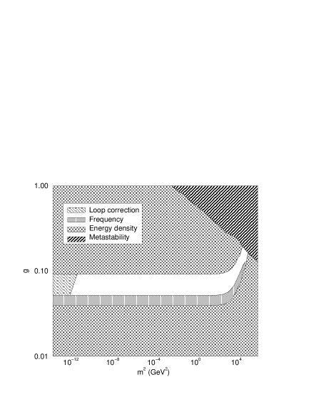
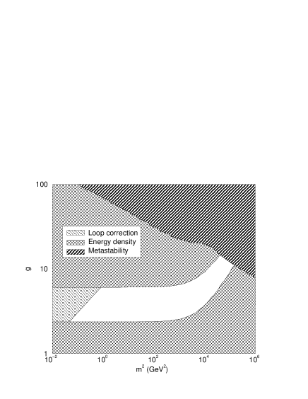
FIG. 2.: The plot of the allowed region of the parameter space. a) $p=5$, $q=6$, b) $p=6$, $q=8$. In this case, we haven’t plotted the frequency contours, because the frequency is almost everywhere very high.

In order to see how much fine tuning of parameters is needed, we show in Fig. 2a the allowed region in $(m^{2},g)$ space. The white region in the plot shows the parameter values than remain allowed after we have excluded the regions ruled out by the metastability constraint (70) the frequency constraint

$$(50~{}{\rm GeV})^{2}<V^{\prime\prime}(\sigma_{\rm min})<(200~{}{\rm GeV})^{2}\ ,$$ (80)

the energy density constraint

$$(150~{}{\rm GeV})^{4}<V_{0}<(300~{}{\rm GeV})^{4}\ ,$$ (81)

and the loop correction constraint [see Eq. (63)]

$$\delta_{\rm loop}<0.1\ .$$ (82)

Of particular note is that around the value $g\approx 0.07$, there is a wide range of allowed values,

$$(1~{}{\rm keV})^{2}\mathrel{\raise 1.29167pt\hbox{$<$}\mkern-14.0mu\lower 2.58334pt\hbox{$\sim$}}m^{2}\mathrel{\raise 1.29167pt\hbox{$<$}\mkern-14.0mu\lower 2.58334pt\hbox{$\sim$}}(300~{}{\rm GeV})^{2}\ .$$ (83)

We have repeated the analysis for other values of the parameters $p$ and $q$, with the result that the constraints become stronger. A natural choice would be $p=6$ and $q=8$, because the potential would then have a $Z_{2}$ symmetry. However, in that case the energy density is typically very high, unless $g$ is large, as shown in Fig. 2b. In such a situation it is questionable whether our techniques can be applied at all. Furthermore, since the frequency of the inflaton oscillations is also typically very high, the inflaton would decay to high-momentum Higgs modes instead of exciting only the lowest modes.

Nevertheless, with $p=5$, $q=6$, the model generates naturally the necessary conditions for the scenario of Refs. [9, 10]. The short-wavelength modes are essentially in vacuum, while the long-wavelength modes have a high effective temperature. When the system thermalizes, this temperature decreases, the system undergoes a non-thermal phase transition to the broken phase [26, 27, 28], and the baryon asymmetry freezes in. Because of the non-perturbative, non-equilibrium nature of the mechanism, reliable estimates for the generated baryon asymmetry can only be obtained by means of numerical simulations, as discussed in Ref. [29]. As an aside, let us point out that because the potential is much more highly curved in the $\sigma$ direction than in the $\phi$ direction (see Fig. 1), the oscillations of $\sigma$ quickly die away, and only $\phi$ keeps oscillating, as was assumed in Ref. [29].

B Baryogenesis from the Kibble Mechanism

If the energy density is lower than is needed for the above scenario, baryogenesis may still take place via the Kibble mechanism as discussed in Section II B. In our model $m^{2}(\sigma)=m^{2}-g^{2}\sigma^{2}$, and the adiabaticity condition (6) implies

$$k_{\rm max}^{3}\sim g^{2}\sigma_{c}\dot{\sigma}.$$ (84)

Using $\sigma_{c}=m/g$, we find

$$n_{\rm configs}\sim\xi_{\rm max}^{-3}\sim k_{\rm max}^{3}\sim gm\dot{\sigma}.$$ (85)

Depending on CP violation, this must be higher than $0.001m_{H}^{3}$ for sufficient baryogenesis [9].

If we insist that inflation does not end before $\sigma_{c}$, the slow-roll condition (11) requires $\dot{\sigma}\ll V(\sigma_{c})^{1/2}\sim m_{H}^{2}$, which may be high enough. We will, however, relax this requirement and assume that inflation has ended before $\sigma_{c}$, whereby we obtain an estimate for the value of $\dot{\sigma}$ by neglecting the expansion of the universe and using conservation of energy. This yields

$$\dot{\sigma}^{2} \sim V(\sigma_{\rm end})-V(\sigma_{c})\sim V_{0}-V(\sigma_{c})$$ (86)

$$= \frac{m_{H}^{4}}{\lambda}\left[\frac{1}{p}\beta\left(\frac{\alpha}{\alpha+1}\right)^{p/2}-\frac{1}{q}\left(\frac{\alpha+1}{4}+\beta\right)\left(\frac{\alpha}{\alpha+1}\right)^{q/2}\right].$$ (87)

In general $\sigma$ will roll past its minimum, reach a maximum value and turn back. If its initial speed is too high and there is not enough friction, it may cross $\sigma_{c}$ again and restore the electroweak symmetry. To avoid this, we require that the energy density is not much higher than is needed for restoring the SU(2) symmetry. In practice, we choose $V_{0}<m_{H}^{4}/4\lambda$. Note, however, that even higher energy densities could be acceptable, because lattice simulations [29] suggest that the Higgs winding changes very reluctantly during symmetry restoration.

The other relevant criteria are the absence of a metastable minimum (70) and that the generated number density of winding configurations is high enough. The white region in Fig. 3a shows the resulting allowed region of parameter space, and is centred around $g\approx 0.2$ and $m^{2}\approx 1000$ GeV².

a)	b)

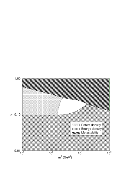
FIG. 3.: a) The region of the parameter space where baryogenesis from the Kibble mechanism is possible. b) The potential at $g=0.2$, $m^{2}=1000$ GeV².

Let us examine these parameters more closely. The couplings become $\lambda_{5}\approx 7.3\times 10^{-5}$ GeV^-1 and $\kappa_{6}\approx 2.4\times 10^{-7}$ GeV^-2, and we also find $\alpha\approx 0.15$, $\beta\approx 0.66$. The potential is shown in Fig. 3b. As can be seen from the plot, even a slight dissipation of energy during the first oscillation means that the field is no longer able to restore the SU(2) symmetry, and any Higgs winding number generated is therefore safe. The speed of the inflaton at $\sigma_{c}$ is

$$\dot{\sigma}(\sigma_{c})\approx 1300~{}{\rm GeV}^{2}\ ,$$ (88)

and the generated winding number density is

$$n_{\rm configs}\approx 8000~{}{\rm GeV}^{3}\approx 0.005m_{H}^{3}\ ,$$ (89)

which may be sufficient for baryogenesis. For an accurate estimate of how $n_{\rm configs}$ relates to $n_{B}/s$, one would have to solve the SU(2)+Higgs equations of motion in the presence of a CP violating coupling.

VI Summary and Conclusions

In this paper we have addressed the fascinating prospect that it may be possible to have successful inflation at the TeV scale, in which the observed fluctuations in the cosmic microwave background are generated. Following the end of this inflation, the observed baryon asymmetry of the universe may then be produced. The self-consistent scenario we have introduced involves an inverted hybrid inflation model which allows us to absorb into the renormalization counterterms of the couplings the potentially dangerous loop corrections present in ordinary hybrid models operating at this low energy scale [18]. The inflaton is directly coupled to the standard model Higgs and during inflation the electroweak symmetry is unbroken. Two possible mechanisms may operate to generate the baryon asymmetry. The first is based on the effective non-thermal restoration of the electroweak symmetry during preheating, which occurs at the end of the inflationary period. During symmetry restoration, the Higgs winding and Chern-Simons numbers can change, and when the system thermalizes, they freeze into a non-zero value. In this mechanism the baryon washout problem of the standard electroweak phase transition is avoided, because the effective cooling rate is determined by the thermalization rate of the standard model fields rather than the expansion of the universe.

The second possibility is through the zero-temperature Kibble mechanism occurring at the end of inflation, when the Higgs field becomes unstable triggering a phase transition. There is no baryon washout problem because the process takes place at zero temperature. The subsequent evolution of the Higgs field leads to configurations being formed in which there is a non-trivial Higgs winding number. These unstable configurations subsequently decay, leading to anomalous fermion number production. Coupled with the fact that the process is out of equilibrium, and assuming there exist CP-violating effects as the configurations unwind, the ingredients are present for the generation of a baryon asymmetry.

In both cases we have presented details showing the degree of fine tuning required to satisfy constraints from both field theory and cosmology. Not surprisingly there is certainly some fine tuning required in these models. For example, it turns out that we require $p=5$ in order to satisfy all the constraints.

It remains to be seen whether such a paradigm is realized in a full, particle physics inspired model of inflation, but it is certainly of potential importance that it appears possible to use the same model to generate both the large scale features of our Universe and the observed baryon asymmetry.

REFERENCES

- [1] V. A. Rubakov and M. E. Shaposhnikov, Usp. Fiz. Nauk166, 493 (1996) [hep-ph/9603208].
- [2] M. Trodden, Rev. Mod. Phys. 71, 1463 (1999) [hep-ph/9803479].
- [3] A. Riotto and M. Trodden, Ann. Rev. Nucl. Part. Sci. 49, 35 (1999) [hep-ph/9901362];
- [4] A. H. Guth, Phys. Rev. D 23, 347 (1981).
- [5] A.D. Linde, Phys. Lett. B 108, 389 (1982).
- [6] A. Albrecht and P.J. Steinhardt, Phys. Rev. Lett. 48, 1220 (1982).
- [7] V. A. Kuzmin, V. A. Rubakov and M. E. Shaposhnikov, Phys. Lett. B155, 36 (1985).
- [8] K. Kajantie, M. Laine, K. Rummukainen and M. Shaposhnikov, Phys. Rev. Lett. 77, 2887 (1996) [hep-ph/9605288].
- [9] L. M. Krauss and M. Trodden, Phys. Rev. Lett. 83, 1502 (1999) [hep-ph/9902420].
- [10] J. Garcia-Bellido, D. Y. Grigoriev, A. Kusenko and M. Shaposhnikov, Phys. Rev. D 60, 123504 (1999) [hep-ph/9902449].
- [11] L. Kofman, A. Linde and A.A. Starobinsky, Phys. Rev. Lett. 73, 3195 (1994).
- [12] J. Traschen and R. Brandenberger, Phys. Rev. D42, 2491 (1990); Y. Shtanov, J. Traschen and R. Brandenberger, Phys. Rev. D51, 5438 (1995).
- [13] D. H. Lyth and A. Riotto, Phys. Rept. 314, 1 (1999) [hep-ph/9807278].
- [14] A. Linde, Particle Physics and Cosmology, section 8.6, (Harwood, Chur, Switzerland, 1990).
- [15] A. Linde and D. Linde, Phys. Rev. D50, 2456 (1994).
- [16] A. Linde, D. Linde and A. Mezhlumian, Phys. Rev. D49, 1783 (1994).
- [17] T. Vachaspati and M. Trodden, Phys. Rev. D 61, 023502 (2000) [gr-qc/9811037].
- [18] D. H. Lyth, Phys. Lett. B466, 85 (1999) [hep-ph/9908219].
- [19] T. W. B. Kibble, J. Phys. A9, 1387 (1976).
- [20] N. Turok and J. Zadrozny, Phys. Rev. Lett. 65, 2331 (1990).
- [21] N. Turok and J. Zadrozny, Nucl. Phys. B358, 471 (1991).
- [22] G. ’t Hooft, Phys. Rev. Lett. 37, 8 (1976).
- [23] A. Lue, K. Rajagopal and M. Trodden, Phys. Rev. D 56, 1250 (1997) [hep-ph/9612282].
- [24] S. Y. Khlebnikov and I. I. Tkachev, Phys. Rev. Lett. 77, 219 (1996) [hep-ph/9603378].
- [25] T. Prokopec and T. G. Roos, Phys. Rev. D 55, 3768 (1997) [hep-ph/9610400].
- [26] L. Kofman, A. Linde and A.A. Starobinsky, Phys. Rev. Lett. 76, 1011 (1996).
- [27] I. I. Tkachev, Phys. Lett. B 376, 35 (1996) [hep-th/9510146].
- [28] A. Rajantie and E. J. Copeland, Phys. Rev. Lett. 85, 916 (2000) [hep-ph/0003025].
- [29] A. Rajantie, P. M. Saffin and E. J. Copeland, Phys. Rev. D 63, 123512 (2001) [hep-ph/0012097].
- [30] J. Garcia-Bellido and A. Linde, Phys. Rev. D 57, 6075 (1998) [hep-ph/9711360].
- [31] G. Felder, J. Garcia-Bellido, P. B. Greene, L. Kofman, A. Linde and I. Tkachev, hep-ph/0012142.
- [32] W. H. Zurek, Acta Phys. Polon. B 24, 1301 (1993).
- [33] M. Hindmarsh and A. Rajantie, Phys. Rev. Lett. 85, 4660 (2000) [cond-mat/0007361].
- [34] A. Linde, Phys. Lett. B 259, 38 (1991).
- [35] E. J. Copeland, A. R. Liddle, D. H. Lyth, E. D. Stewart and D. Wands, Phys. Rev. D 49, 6410 (1994) [astro-ph/9401011].
- [36] N. Kaloper and A. Linde, Phys. Rev. D 59, 101303 (1999) [hep-th/9811141].
- [37] B. A. Ovrut and P. J. Steinhardt, Phys. Rev. Lett. 53, 732 (1984).
- [38] D. H. Lyth and E. D. Stewart, Phys. Rev. D 54, 7186 (1996) [hep-ph/9606412].
- [39] M. Bastero-Gil and S. F. King, Phys. Lett. B 423, 27 (1998) [hep-ph/9709502].
- [40] D. H. Lyth, Phys. Lett. B 488, 417 (2000) [hep-ph/9911257].
- [41] M. E. Shaposhnikov, JETP Lett. 44, 465 (1986).
- [42] M. E. Shaposhnikov, Nucl. Phys. B287, 757 (1987).
- [43] R. Barate et al. [ALEPH Collaboration], Phys. Lett. B 495, 1 (2000) [hep-ex/0011045]; M. Acciarri et al. [L3 Collaboration], Phys. Lett. B 495, 18 (2000) [hep-ex/0011043].